Learning Quickly to Plan Quickly Using Modular Meta-Learning

Abstract

Multi-object manipulation problems in continuous state and action spaces can be solved by planners that search over sampled values for the continuous parameters of operators. The efficiency of these planners depends critically on the effectiveness of the samplers used, but effective sampling in turn depends on details of the robot, environment, and task. Our strategy is to learn functions called specializers that generate values for continuous operator parameters, given a state description and values for the discrete parameters. Rather than trying to learn a single specializer for each operator from large amounts of data on a single task, we take a modular meta-learning approach. We train on multiple tasks and learn a variety of specializers that, on a new task, can be quickly adapted using relatively little data – thus, our system learns quickly to plan quickly using these specializers. We validate our approach experimentally in simulated 3D pick-and-place tasks with continuous state and action spaces. Visit http://tinyurl.com/chitnis-icra-19 for a supplementary video.

I Introduction

Imagine a company that is developing software for robots to be deployed in households or flexible manufacturing situations. Each of these settings might be fairly different in terms of the types of objects to be manipulated, the distribution over object arrangements, or the typical goals. However, they all have the same basic underlying kinematic and physical constraints, and could in principle be solved by the same general-purpose task and motion planning (tamp) system. Unfortunately, tamp is highly computationally intractable in the worst case, involving a combination of search in symbolic space, search for motion plans, and search for good values for continuous parameters such as object placements and robot configurations that satisfy task requirements.

A robot faced with a distribution over concrete tasks can learn to perform tamp more efficiently by adapting its search strategy to suit these tasks. It can learn a small set of typical grasps for the objects it handles frequently, or good joint configurations for taking objects out of a milling machine in its workspace. This distribution cannot be anticipated by the company for each robot, so the best the company can do is to ship robots that are equipped to learn very quickly once they begin operating in their respective new workplaces.

The problem faced by this hypothetical company can be framed as one of meta-learning: given a set of tasks drawn from some meta-level task distribution, learn some structure or parameters that can be used as a prior so that the robot, when faced with a new task drawn from that same distribution, can learn very quickly to behave effectively.

Concretely, in this work we focus on improving the interface between symbolic aspects of task planning and continuous aspects of motion planning. At this interface, given a symbolic plan structure, it is necessary to select values for continuous parameters that will make lower-level motion planning queries feasible, or to determine that the symbolic structure itself is infeasible. Typical strategies are to search over randomly sampled values for these parameters, or to use hand-coded “generators” to produce them [1, 2].

Our strategy is to learn deterministic functions, which we call specializers, that map a symbolic operator (such as place(objA)) and a detailed world state description (including object shapes, sizes, poses, etc.) into continuous parameter values for the operator (such as a grasp pose). Importantly, rather than focusing on learning a single set of specializers from a large amount of data at deployment time, we will focus on meta-learning approaches that allow specializers to be quickly adapted online. We will use deep neural networks to represent specializers and backpropagation to train them.

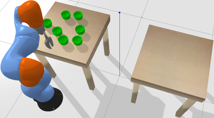
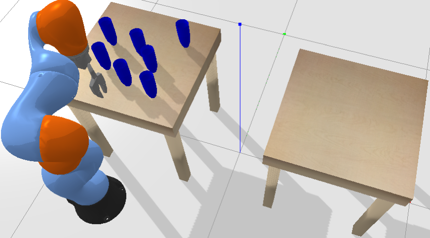
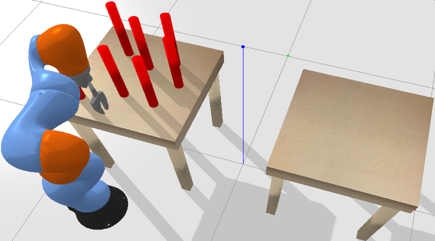
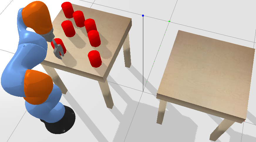
Figure 1: We address the problem of learning values for continuous action parameters in task and motion planning. We take a modular meta-learning approach, where we train functions across multiple tasks to generate these values, by interleaving planning and optimization. Pictured are three of our tabletop manipulation tasks used for training and one used for evaluation (bottom right). Object shapes and sizes vary across tasks, affecting how the robot should choose grasp and place poses. On an evaluation task, the robot is given a small amount of data – it must learn quickly to plan quickly, adapting its learned functions to generate good target poses.

We compare two different modular meta-learning strategies: one, based on maml [3], focuses on learning neural network weights that can be quickly adapted via gradient descent in a new task; the other, based on BounceGrad [4], focuses on learning a fixed set of neural network “modules” from which we can quickly choose a subset for a new task.

We demonstrate the effectiveness of these approaches in an object manipulation domain, illustrated in Figure 1, in which the robot must move all of the objects from one table to another. This general goal is constant across tasks, but different tasks will vary the object shapes and sizes, requiring the robot to learn to manipulate these different types of objects. We conjecture that the meta-learning approach will allow the robot, at meta-training time, to discover generally useful, task-independent strategies, such as placing objects near the back of the available space; and, at deployment time, to quickly learn to adapt to unseen object geometries. Our methods are agnostic to exactly which aspects of the environments are common to all tasks and which vary – these concepts are naturally discovered by the meta-learning algorithm. We show that the meta-learning strategies perform better than both a random sampler and a reasonable set of hand-built, task-agnostic, uninformed specializers.

II Related Work

Our work is focused on choosing continuous action parameters within the context of a symbolic plan. We are not learning control policies for tasks [5, 6, 7], nor are we learning planning models of tasks [8]. We assume any necessary policies and planning models exist; our goal is to make planning with such models more efficient by learning specializers via modular meta-learning. There is existing work on learning samplers for continuous action parameters in task and motion planning [9, 10, 11, 12], but these methods do not explicitly consider the problem of learning samplers that can be quickly adapted to new tasks.

Meta-Learning: Meta-learning is a particularly important paradigm for learning in robotics, where training data can be very expensive to acquire, because it dramatically lowers the data requirements for learning new tasks. Although it has a long history in the transfer learning literature [13], meta-learning was recently applied with great effectiveness to problems in robotics by Finn et al. [3].

Learning Modular Structure: Our approach is a modular learning approach, in the sense of Andreas et al. [14]: the specializers we learn are associated with planning operators, allowing them to be recombined in new ways to solve novel problems. Andreas et al. [15] use reinforcement learning to train subtask modules in domains with decomposable goals. Unlike in our work, they assume a policy sketch is given.

Modular Meta-Learning: Modular meta-learning was developed by Alet et al. [4] and forms the inspiration for this work. Their work includes an EM-like training procedure that alternates between composing and optimizing neural network modules, and also includes a mechanism for choosing the best compositional structure of the modules to fit a small amount of training data on a new task.

III Problem Setting

III-A Task and Motion Planning

Robot task and motion (tamp) problems are typically formulated as discrete-time planning problems in a hybrid discrete-continuous state transition system [16, 17], with discrete variables modeling which objects are being manipulated and other task-level aspects of the domain, and continuous variables modeling the robot configuration, object poses, and other continuous properties of the world.

A world state $s\in\mathcal{S}$ is a complete description of the state of the world, consisting of $(c,o^{1},\ldots,o^{n},x^{1},\ldots,x^{m})$, where $c$ is the robot configuration, the $o^{i}$ are the states of each object in the domain, and the $x^{i}$ are other discrete or continuous state variables. Each object’s state is $d$-dimensional and describes its properties, such as mass or color.

We now define a tamp problem, using some definitions from Garrett et al. [16]. A predicate is a Boolean function. A fluent is an evaluation of a predicate on a tuple $(\bar{o},\bar{\theta})$, where $\bar{o}$ is a set of discrete objects and $\bar{\theta}$ is a set of continuous values. A set of basis predicates $B$ can be used to completely describe a world state. Given a world state $s$, the set of basis fluents $\Phi_{B}(s)$ is the maximal set of atoms that are true in $s$ and can be constructed from the basis predicate set $B$. A set of derived predicates can be defined in terms of basis predicates. A planning state $\mathcal{I}$ is a set of fluents, including a complete set of basis fluents and any number of derived fluents; it is assumed that any fluent not in $\mathcal{I}$ is false.

An action or operator $a$ is given by an argument tuple $\bar{O}=(O_{1},\ldots,O_{v})$, a parameter tuple $\bar{\Theta}=(\Theta_{1},\ldots,\Theta_{w})$, a set of fluent preconditions ${\it pre}(a)$ on $(\bar{O},\bar{\Theta})$, and a set of positive and negative fluent effects ${\it eff}(a)$ on $(\bar{O},\bar{\Theta})$. An action instance $a(\bar{o},\bar{\theta})$ is an action $a$ with arguments and parameters $(\bar{O},\bar{\Theta})$ replaced with discrete objects $\bar{o}$ and continuous values $\bar{\theta}$. An action instance $a(\bar{o},\bar{\theta})$ is applicable in planning state $\mathcal{I}$ if ${\it pre}(a(\bar{o},\bar{\theta}))\subseteq\mathcal{I}$. The result of applying an action instance $a(\bar{o},\bar{\theta})$ to a planning state $\mathcal{I}$ is a new state $\mathcal{I}\cup{\it eff}^{+}(a(\bar{o},\bar{\theta}))\setminus{\it eff}^{-}(a(\bar{o},\bar{\theta}))$, where ${\it eff}^{+}$ and ${\it eff}^{-}$ are the positive and negative fluents in ${\it eff}$, respectively. For $a$ to be a well-formed action, ${\it eff}^{+}(a)$ and ${\it eff}^{-}(a)$ must be structured so that the planning state ${\mathcal{I}}^{\prime}$ resulting from applying $a$ is valid (contains a complete set of basis fluents). Then, $\mathcal{I^{\prime}}$ determines a world state $s\in\mathcal{S}$, and the action $a$ can be viewed as a deterministic transition on world states.

A tamp problem $({\mathcal{A}},\mathcal{I},{\mathcal{G}})$ is given by a set of actions ${\mathcal{A}}$, an initial planning state $\mathcal{I}$, and a goal set of fluents ${\mathcal{G}}$. A sequence of action instances, $\pi=\langle a_{1}(\bar{o}_{1},\bar{\theta}_{1}),\ldots a_{k}(\bar{o}_{k},\bar{\theta}_{k})\rangle$, is called a plan. A plan $\pi$ is a task-level solution for problem $({\mathcal{A}},\mathcal{I},{\mathcal{G}})$ if $a_{1}(\bar{o}_{1},\bar{\theta}_{1})$ is applicable in $\mathcal{I}$, each $a_{i}(\bar{o}_{i},\bar{\theta}_{i})$ is applicable in the $(i-1)$th state resulting from application of the previous actions, and ${\mathcal{G}}$ is a subset of the final state. A plan skeleton $\hat{\pi}$ is a sequence of actions whose discrete arguments are instantiated but continuous parameters are not: $\hat{\pi}=\langle a_{1}(\bar{o}_{1},\bar{\Theta}_{1}),\ldots a_{k}(\bar{o}_{k},\bar{\Theta}_{k})\rangle$.

A world-state trajectory $\tau(\pi,\mathcal{I})$ is the sequence of world states $s_{1},\ldots,s_{k}\in\mathcal{S}$ induced by the sequence of planning states $\mathcal{I}_{1},...,\mathcal{I}_{k}$ resulting from applying plan $\pi$ starting from $\mathcal{I}$. A task-level solution $\pi$ is a complete solution for the tamp problem $({\mathcal{A}},\mathcal{I},{\mathcal{G}})$ if, letting $\tau(\pi,\mathcal{I})=\langle s_{1},\ldots s_{k}\rangle$, there exist robot trajectories $\tilde{\tau}_{1},\ldots,\tilde{\tau}_{k-1}$ such that $\tilde{\tau}_{i}$ is a collision-free path (a motion plan) from $c_{i}$ to $c_{i+1}$, the robot configurations in world states $s_{i}$ and $s_{i+1}$ respectively.

III-B Solving Task and Motion Planning Problems

Finding good search strategies for solving tamp problems is an active area of research, partly owing to the difficulty of finding good continuous parameter values that produce a complete solution $\pi$. Our meta-learning method could be adapted for use in many tamp systems, but for clarity we focus on the simple one sketched below. See Section V for discussion of the tamp system we use in our implementation.

Algorithm PlanSketch$(\mathcal{A},\mathcal{I},\mathcal{G})$

     1 for $\hat{\pi}$ in some enumeration of plan skeletons do

          2 for $\bar{\theta}$ s.t. $\pi=\hat{\pi}(\bar{\theta})$ is a task-level solution do

               3 if motion plans exist for $\pi$ then

                     return the complete solution $\pi$

                    

                    

                    

The problems of symbolic task planning to yield plausible plan skeletons (Line 1) and collision-free motion planning (Line 3) are both well-studied, and effective solutions exist. We focus on the problem of searching over continuous values $\bar{\theta}$ for the skeleton parameters (Line 2).

We first outline two simple strategies for finding $\bar{\theta}$. In random sampling, we perform a simple depth-first backtracking search: sample values for $\theta_{i}$ uniformly at random from some space, check whether there is a motion plan from $s_{i-1}$ to $s_{i}$, continue on to sample $\theta_{i+1}$ if so, and either sample $\theta_{i}$ again or backtrack to a higher node in the search tree if not. In the hand-crafted strategy, we rely on a human programmer to write one or more specializers $\sigma_{a}^{i}$ for each action $a$. A specializer is a function $\sigma(\mathcal{I},\bar{o},j)$, where $\mathcal{I}$ is a planning state, $\bar{o}$ are the discrete object arguments with which $a$ will be applied, and $j$ is the step of the skeleton where a particular instance of $a$ occurs. The specializer $\sigma$ returns a vector of continuous parameter values $\bar{\theta}$ for $a$. So, in this hand-crafted strategy, for each plan skeleton $\hat{\pi}$ we need only consider the following discrete set of plans $\pi$:

$$\pi=\langle a_{1}(\bar{o}_{1},\sigma^{i_{1}}_{a_{1}}(\mathcal{I}_{1},\bar{o}_{1},1)),\ldots a_{k}(\bar{o}_{k},\sigma^{i_{k}}_{a_{k}}(\mathcal{I}_{k},\bar{o}_{k},k))\rangle\;\;,$$

where the $i$ values select which specializer to use for each step. Each setting of the $i$ values yields a different plan $\pi$.

Now, it is sensible to combine the search over both skeletons and specializers into a single discrete search. Let $\Sigma(W)$ be a set of specializers (the reason for this notation will become clear in the next section) and $\mathcal{A}(\Sigma(W))$ be a discrete set of “actions” obtained by combining each action $a\in\mathcal{A}$ with each specializer $\sigma_{a}^{i}\in\Sigma(W)$, indexed by $i$. We obtain our algorithm for planning with specializers:

Algorithm Plan$(\mathcal{A},\mathcal{I},\mathcal{G},\Sigma(W))$

     1 for $\pi$ in $\textsc{SymbolicPlan}(\mathcal{A}(\Sigma(W)),\mathcal{I},\mathcal{G})$ do

          2 if motion plans exist for $\pi$ then

                return the complete solution $\pi$

               

               

III-C Learning Specializers

We begin by defining our learning problem for just a single task. A single-task specializer learning problem is a tuple $({\mathcal{A}},\mathcal{D},\Sigma(W))$, where ${\mathcal{A}}$ is a set of actions specifying the dynamics of the domain, $\mathcal{D}=\{(\mathcal{I}_{1},{\mathcal{G}}_{1}),\ldots,(\mathcal{I}_{n},{\mathcal{G}}_{n})\}$ is a dataset of (initial state, goal) problem instances, $\Sigma$ is a set of functional forms for specializers (such as neural network architectures), and $W$ is a set of initial weights such that $\Sigma(W)$ is a set of fully instantiated specializers that can be used for planning with the Plan algorithm.

The objective of our learning problem is to find $W$ such that planning with $\Sigma(W)$ will, in expectation over new $(\mathcal{I},{\mathcal{G}})$ problem instances drawn from the same distribution as $\mathcal{D}$, be likely to generate complete solutions. The functional forms $\Sigma$ of the specializers are given (just like in the hand-crafted strategy), but the weights $W$ are learned.

Although our ultimate objective is to improve the efficiency of the overall planner, that is done by replacing the search over continuous parameter values $\bar{\theta}$ with a deterministic choice or search over a finite set of parameter values provided by the specializers; so, our objective is really that these specializers be able to solve problems from $\mathcal{D}$.

Most directly, we could try to minimize $0-1$ single-task loss on $\mathcal{D}$, so that $W^{*}=\operatorname*{argmin}_{W}\mathcal{L}_{S}(W;\mathcal{D})$ where:

$$\mathcal{L}_{S}(W;\mathcal{D})=\sum_{(\mathcal{I},\mathcal{G})\in\mathcal{D}}\begin{cases}0&\text{$\text{\sc Plan}(\mathcal{A},\mathcal{I},\mathcal{G},\Sigma(W))$ succeeds}\\ 1&\text{otherwise}\end{cases}$$

Unfortunately, this loss is much too difficult to optimize in practice; in Section IV-A we will outline strategies for smoothing and approximating the objective.

III-D Meta-Learning Specializers

In meta-learning, we wish to learn, from several training tasks, some form of a prior that will enable us to learn to perform well quickly on a new task. A specializer meta-learning problem, given by a tuple $({\mathcal{A}},(\mathcal{D}_{1},\ldots,\mathcal{D}_{m}),\Sigma(W))$, differs from a single-task specializer learning problem both in that it has multiple datasets $\mathcal{D}_{j}$, and in that it has a different objective. We make the implicit assumption, standard in meta-learning settings, that there is a hierarchical distribution over $(\mathcal{I},{\mathcal{G}})$ problems that the robot will encounter: we define a task to be a single distribution over $(\mathcal{I},\mathcal{G})$, and we assume we have a distribution over tasks.

Let $\text{\sc Learn}({\mathcal{A}},\mathcal{D},\Sigma(W))$ be a specializer learning algorithm that returns $W^{*}$, tailored to work well on problems drawn from $\mathcal{D}$. Our meta-learning objective will then be to find a value of $W$ that serves as a good prior for Learn on new tasks, defined by new $(\mathcal{I},{\mathcal{G}})$ distributions. Formally, the meta-learning objective is to find $W^{*}_{M}=\operatorname*{argmin}_{W}\mathcal{L}_{M}(W)$, where the meta-learning loss is, letting $j$ index over tasks:

$$\mathcal{L}_{M}(W)=\frac{1}{m}\sum_{j=1}^{m}\mathcal{L}_{S}(\text{\sc Learn}(\mathcal{A},\mathcal{D}_{j}^{\rm train},\Sigma(W));\mathcal{D}_{j}^{\rm test})\;\;.$$

The idea is that a new set of weights obtained by starting with $W$ and applying Learn on a training set from task $j$ should perform well on a held-out test set from task $j$.

After learning $W^{*}_{M}$, the robot is deployed. When it is given a small amount of training data $\mathcal{D}_{\rm new}$ drawn from a new task, it will call $\text{\sc Learn}(\mathcal{A},\mathcal{D}_{\rm new},\Sigma(W^{*}_{M}))$ to get a new set of weights $W^{*}_{\rm new}$, then use the planner $\text{\sc Plan}(\mathcal{A},\mathcal{I},\mathcal{G},\Sigma(W^{*}_{\rm new}))$ to solve future problem instances $(\mathcal{A},\mathcal{I},\mathcal{G})$ from this new task. If the meta-learning algorithm is effective, it will have learned to

• learn quickly (from a small dataset $\mathcal{D}_{\rm new}$) to

• plan quickly (using the specializers $\Sigma(W^{*}_{\rm new})$ in place of a full search over continuous parameter values $\bar{\theta}$),

motivating our title.

IV Algorithms

In this section, we begin by describing two single-task specializer learning algorithms, and then we discuss a specializer meta-learning algorithm that can be used with any specializer learning algorithm.

IV-A Single-Task Specializer Learning Algorithms

Recall that an algorithm for learning specializers takes as input $({\mathcal{A}},\mathcal{D},\Sigma(W))$, and its job is to return $W^{*}=\operatorname*{argmin}_{W}\mathcal{L}_{S}(W;\mathcal{D})$. We consider two algorithms: alternating descent (ad) and subset selection (ss).

a) Alternating Descent: ad adjusts the weights $W$ to tune them to dataset $\mathcal{D}$.

If we knew, for each $({\mathcal{I}},{\mathcal{G}})\in\mathcal{D}$, the optimal plan skeleton and choices of specializers that lead to a complete solution $\pi$ for the tamp problem $({\mathcal{A}},{\mathcal{I}},{\mathcal{G}})$, then we could adjust the elements of $W$ corresponding to the chosen specializers in order to improve the quality of $\pi$. However, this optimal set of actions and specializers is not known, so we instead perform an EM-like alternating optimization. In particular, we use the PlanT algorithm (described in detail later), an approximation of Plan that can return illegal plans, to find a skeleton $\hat{\pi}$ and sequence of specializers $\sigma_{j}$ to be optimized. Then, we adjust the elements of $W$ corresponding to the $\sigma_{j}$ to make the plan “less illegal.”

Formally, we assume the existence of a predicate loss function $\mathcal{L}_{p}$ for each predicate $p$ in the domain, which takes in the arguments of predicate $p$ ($\bar{o}$ and $\bar{\theta}$) and a world state $s\in\mathcal{S}$, and returns a positive-valued loss measuring the degree to which the fluent $p(\bar{o},\bar{\theta})$ is violated in $s$. If $p(\bar{o},\bar{\theta})$ is true in $s$, then $\mathcal{L}_{p}(\bar{o},\bar{\theta},s)$ must be zero. For example, if fluent $\phi={\rm pose}(o,v)$ asserts that the pose of object $o$ should be the value $v$, then we might use the squared distance $(v-v^{\prime})^{2}$ as the predicate loss, where $v^{\prime}$ is the actual pose of $o$ in $s$.

Now consider the situation in which we run PlanT, and it returns a plan $\pi$ created from a plan skeleton $\hat{\pi}$ and the chosen specializers $\sigma_{1},\ldots,\sigma_{k}$. From this, we can compute both the induced trajectory of planning states ${\mathcal{I}_{1}},\ldots,{\mathcal{I}_{k}}$, and the induced trajectory of world states $\tau=\langle s_{1},\ldots s_{k}\rangle$. We can now define a trajectory loss function $\mathcal{L}_{\tau}$ on $W$ for $\pi$:

$$\mathcal{L}_{\tau}(W;\mathcal{I},\mathcal{G},\pi)=\sum_{j=1}^{k}\sum_{\phi\in{\it eff}^{+}(a_{j}(\bar{o}_{j},\bar{\theta}_{j}))}\mathcal{L}_{p(\phi)}(\bar{o}_{j},\bar{\theta}_{j},s_{j})\;\;.$$

This is a sum over steps $j$ in the plan, and for each step, a sum over positive fluents $\phi$ in its effects, of the degree to which that fluent is violated in the resulting world state $s_{j}$. Here, $p(\phi)$ is the predicate associated with fluent $\phi$. Recall that $\bar{\theta}_{j}=\sigma_{j}(\mathcal{I}_{j},\bar{o}_{j},j;W)$, where we have included $W$ to expose the specializers’ parametric forms. Thus, we have:

$$\mathcal{L}_{\tau}(W;\mathcal{I},\mathcal{G},\pi)=\sum_{j=1}^{k}\sum_{\phi}\mathcal{L}_{p(\phi)}(\bar{o}_{j},\sigma_{j}(\mathcal{I}_{j},\bar{o}_{j},j;W),s_{j})\;\;.$$

If the $\mathcal{L}_{p}$ are differentiable with respect to the $\bar{\theta}$, and the functional forms $\Sigma$ generating the $\bar{\theta}$ are differentiable with respect to $W$ and their continuous inputs, then $W$ can be adjusted via a gradient step to reduce $\mathcal{L}_{\tau}$. This method will adjust only the values of $W$ that were used in the specializers chosen by PlanT. The overall algorithm is:

Algorithm AD-Learn$(\mathcal{A},\mathcal{D},\Sigma(W),n_{\rm iters},n_{\rm plans})$

      1 for $t=1$ to $n_{\rm iters}$ do

            2 Sample $(\mathcal{I},\mathcal{G})$ from $\mathcal{D}$.

            3 $\pi\leftarrow$ PlanT$(\mathcal{A},\mathcal{I},\mathcal{G},\Sigma(W),t,n_{\rm plans})$

            4 $W\leftarrow W-\alpha\nabla_{W}\mathcal{L}_{\tau}(W;\mathcal{I},\mathcal{G},\pi)$

            

Subroutine PlanT$(\mathcal{A},\mathcal{I},\mathcal{G},\Sigma(W),t,n_{\rm plans})$

      5 for $i=1$ to $n_{\rm plans}$ do

            6 $\pi_{i}\leftarrow{\rm next}\;\textsc{SymbolicPlan}(\mathcal{A}(\Sigma(W)),\mathcal{I},\mathcal{G})$

            7 if motion plans exist for $\pi_{i}$ then

                  8 ${\rm score}(\pi_{i})\leftarrow-\mathcal{L}_{\tau}(W;\mathcal{I},\mathcal{G},\pi_{i})$

      9if no scores were computed then

            10 Randomly initialize more specializers; repeat.

      11return sample $\pi_{i}\sim e^{{\rm score}(\pi_{i})/T(t)}/Z$

We now describe in detail the PlanT procedure, which is an approximation of Plan. Generally, while we are learning $W$, we will not have a complete and correct set of specializers, but we still need to assemble plans in order to adjust the $W$. In addition, to prevent local optima, and inspired by the use of simulated annealing for structure search in BounceGrad [4] and moma [4], we do not always consider the $\pi$ with least loss early on. PlanT, rather than trying to find a $\pi$ that is a complete solution for the tamp problem, treats SymbolicPlan as a generator, generates $n_{\rm plans}$ symbolic plans that are not necessarily valid solutions, and for each one that is feasible with respect to motion planning, computes its loss. It then samples a plan to return using a Boltzmann distribution derived from the losses, with “temperature” parameter $T(t)$ computed as a function of the number of optimization steps done so far. This $T(t)$ should be chosen to go to zero as $t$ increases.

b) Subset Selection: ss assumes that $\Sigma(W)$ includes a large set of specializers, and simply selects a subset of them to use during planning, without making any adjustments to the weights $W$. Let $\Sigma_{a}(W)$ be the set of specializers for action $a$ and integer $k$ be a parameter of the algorithm. The ss algorithm simply finds, for each action $a$, the size-$k$ subset $\rho_{a}$ of $\Sigma_{a}(W)$ such that $\mathcal{L}_{S}(\cup_{a}\rho_{a};\mathcal{D})$ is minimized. There are many strategies for finding such a set; in our experiments, we have a small number of actions and set $k=1$, and so we can exhaustively evaluate all possible combinations.

IV-B Specializer Meta-Learning Algorithm

Recall that an algorithm for meta-learning specializers takes as input $({\mathcal{A}},(\mathcal{D}_{1},\ldots,\mathcal{D}_{m}),\Sigma(W))$, and its job is to return $W^{*}_{M}=\operatorname*{argmin}_{W}\mathcal{L}_{M}(W)$, which should be a good starting point for learning in a new task. This ideal objective is difficult to optimize, so we must make approximations.

We begin by describing the meta-learning algorithm, which follows a strategy very similar to maml [3]. We do stochastic gradient descent in an outer loop: draw a task $\mathcal{D}_{j}$ from the task distribution, use some learning algorithm Learn to compute a new set of weights $W_{j}$ for $\mathcal{D}_{j}^{\rm train}$ starting from $W$, and update $W$ with a gradient step to reduce the trajectory loss on $D_{j}^{\rm test}$ evaluated using $W_{j}$.

Algorithm MetaLearn$(\mathcal{A},\mathcal{D}_{1},\ldots,\mathcal{D}_{m},\Sigma(W))$

      1 while not done do

            2 $j\leftarrow{\rm sample}(1,\ldots,m)$

            3 $W_{j}\leftarrow\text{\sc Learn}(\mathcal{A},\mathcal{D}_{j}^{\rm train},\Sigma(W))$

            4 $W\leftarrow W-\beta\nabla_{W}\mathcal{L}_{\tau,\mathcal{D}_{j}^{\rm test}}(\Sigma(W_{j}))$

            

For efficiency, in practice we drop the Hessian term in the gradient by taking the gradient with respect to $W_{j}$ (so $\nabla_{W}\to\nabla_{W_{j}}$). This is an approximation that is successfully made by several maml implementations. We define:

$$\mathcal{L}_{\tau,\mathcal{D}}(\Sigma(W))=\sum_{\mathcal{I},\mathcal{G}\in\mathcal{D}}\mathcal{L}_{\tau}(W;\mathcal{I},\mathcal{G},\text{\sc PlanT}(\mathcal{A},\mathcal{I},\mathcal{G},\Sigma(W),\infty,\infty)).$$

This expression gives the smoothed trajectory loss for the best plan we can find using the given $\Sigma(W)$, summed over all planning problems in $\mathcal{D}$. When we compute the gradient, we ignore the dependence of the plan structure on $W$. Thus, we estimate $\nabla_{W_{j}}\mathcal{L}_{\tau,\mathcal{D}_{j}^{\rm test}}(\Sigma(W_{j}))$ as follows:

1 for $t=1$ to $n_{\rm gradEst}$ do

      2 Sample $(\mathcal{I},\mathcal{G})$ from $\mathcal{D}_{j}^{\rm test}$.

      3 $\pi\leftarrow$ PlanT$(\mathcal{A},\mathcal{I},\mathcal{G},\Sigma(W_{j}),\infty,\infty)$

      4 $\nabla_{W_{j}}\leftarrow\nabla_{W_{j}}+\nabla_{W_{j}}\mathcal{L}_{\tau}(W_{j};\mathcal{I},\mathcal{G},\pi)$

      

5return $\nabla_{W_{j}}$

When Learn is the subset selection learner (ss), the Learn procedure returns only a subset of the $\Sigma(W)$, corresponding to the chosen specializers. Only the weights in that subset are updated with a gradient step on the test data.

V Experiments

We demonstrate the effectiveness of our approach in a simulated object manipulation domain where the robot is tasked with moving all objects from one table to another, as shown in Figure 1. The object geometries vary across tasks, while a single task is a distribution over initial configurations of the objects on the starting table. We consider 6 training tasks and 3 evaluation tasks, across 3 object types: cylinders, bowls, and vases. The phrase “final task” henceforth refers to a random sample of one of the 3 evaluation tasks.

We use a KUKA iiwa robot arm. Grasp legality is computed using a simple end effector pose test based on the geometry of the object being grasped. We require that cylinders are grasped from the side, while bowls and vases are grasped from above, on their lip. There are four operators: moveToGrasp and moveToPlace move the robot (and any held object) to a configuration suitable for grasping or placing an object, grasp picks an object up, and place places it onto the table. All operators take in the ID of the object being manipulated as a discrete argument. The continuous parameters learned by our specializers are the target end effector poses for each operator; we use an inverse kinematics solver to try reaching these poses.

We learn three specializers for each of the first three operators, and one specializer for place due to its relative simplicity. The state representation is a vector containing the end effector pose, each object’s position, object geometry information, robot base position, and the ID of the currently-grasped object (if any). Thus, we are assuming a fully observed closed world with known object poses, in order to focus on the meta-learning aspect of this setting.

All specializers are fully connected, feedforward neural networks with hidden layer sizes [100, 50, 20], a capacity which preliminary experiments found necessary. We use batch size 32 and the Adam optimizer [18] with initial learning rate $10^{-2}$, decaying by 10% every 1000 iterations.

For motion planning, we use the RRT-Connect algorithm [19]; we check for infeasibility crudely by giving the algorithm a computation allotment, implemented as a maximum number of random restarts to perform, upon which a (infeasible) straight-line trajectory is returned. We use Fast-Forward [20] as our symbolic planner. For simulation and visualization, we use the pybullet [21] software.

A major source of difficulty in this domain is that the end effector poses chosen by the specializers must be consistent with both each other (place pose depends on grasp pose, etc.) and the object geometries. Furthermore, placing the first few objects near the front of the goal table would impede the robot’s ability to place the remaining objects. We should expect that the general strategies discovered by our meta-learning approach would handle these difficulties.

To implement the discrete search over plan skeletons and specializers, we adopt the tamp approach of Srivastava et al. [2], which performs optimistic classical planning using abstracted fluents, attempts to find a feasible motion plan, and incorporates any infeasibilities back into the initial state as logical fluents. For each skeleton, we search exhaustively over all available specializers for each operator.

Evaluation: We evaluate the MetaLearn algorithm with both the alternating descent (ad) learner and the subset selection (ss) learner. We test against two baselines, random sampling and the hand-crafted strategy, both of which are described in Section III-B. The random sampler is conditional, sampling only end effector poses that satisfy the kinematic constraints of the operators. At final task time with the ad learner, we optimize the specializers on 10 batches of training data, then evaluate on a test set of 50 problems from this task. At final task time with the ss learner, we choose a subset of $k=1$ specializer per operator that performs the best over one batch of training data, then use only that subset to evaluate on a test set. Note that we should expect the test set evaluation to be much faster with the ss learner than with the ad learner, since we are planning with fewer specializers.

Setting	System	Final Task Solve %	Train Iters to 50%	Search Effort	Train Time (Hours)
3 obj.	Baseline: Random	24	N/A	52.2	N/A
3 obj.	Baseline: Hand-crafted	68	N/A	12.1	N/A
3 obj.	Meta-learning: ad	100	500	2.5	4.3
3 obj.	Meta-learning: ss	100	500	2.0	0.6
5 obj.	Baseline: Random	14	N/A	81.3	N/A
5 obj.	Baseline: Hand-crafted	44	N/A	34.3	N/A
5 obj.	Meta-learning: ad	88	2.1K	8.6	7.4
5 obj.	Meta-learning: ss	72	6.8K	4.1	1.5
7 obj.	Baseline: Random	0	N/A	N/A	N/A
7 obj.	Baseline: Hand-crafted	18	N/A	64.0	N/A
7 obj.	Meta-learning: ad	76	5.1K	18.3	12.3
7 obj.	Meta-learning: ss	54	9.2K	7.8	2.1

TABLE I: Summary of experimental results. Percentage of 50 final task problem instances solved within a 30-second timeout, number of meta-training iterations needed to reach 50% final task solve rate, average number of plan skeletons and specializers searched over, and total training time in hours. Both meta-learning approaches learn to perform much better at the final task than the baselines do. Notably, the alternating descent (ad) learner performs better than the subset selection (ss) learner, likely because in the former, the specializer weights are optimized for the final task rather than held fixed. However, this improvement comes at the cost of much longer training times. Meta-learners were trained for $10^{4}$ iterations.

Results & Discussion Table I and Figure 2 show that both meta-learning approaches perform much better at the final task than the baselines do. The random sampler fails because it expends significant effort trying to reach infeasible end effector poses, such as those behind the objects. The hand-crafted specializers, though they perform better than the random sampler, suffer from a lack of context: because they are task-agnostic, they cannot specialize, and so search effort is wasted on continuous parameter values that are inappropriate for the current task, making timeouts frequent. Furthermore, the hand-crafted strategy does not adapt to the state (e.g., the locations of objects around one being grasped).

Qualitatively, we found that the general strategies we outlined earlier for succeeding in this domain were meta-learned by our approach (see video linked in abstract).

Notably, the alternating descent (ad) learner performs better than the subset selection (ss) learner, likely because in the former, the specializer weights are optimized for the final task rather than held fixed. These findings suggest that this sort of fine-tuning is an important step to learning specializers in this domain. However, this improvement comes at the cost of much longer training times, since the ad learner performs an inner gradient computation which the ss learner does not; the ad learner may be impractical in larger domains without introducing heuristics to guide the search. Another finding is that the ss learner expends much less search effort than the ad learner, as expected.

Figure 3 (left) shows the benefit of learning in the final task when starting from meta-trained specializers. The specializers meta-learned using the ad learner start off slightly worse than those meta-learned using the ss learner, likely because the search space is larger (recall that the ad learner uses all the specializers), so timeouts are more frequent. After some adaptation on the final task, the ad learner performs better. Figure 3 (right) suggests that when the agent has access to more training tasks, it meta-learns specializers that lead to better final task performance, given a fixed amount of data in this final task. This is likely because each new training task allows the agent to learn more about how to adapt its specializers to the various object geometries.

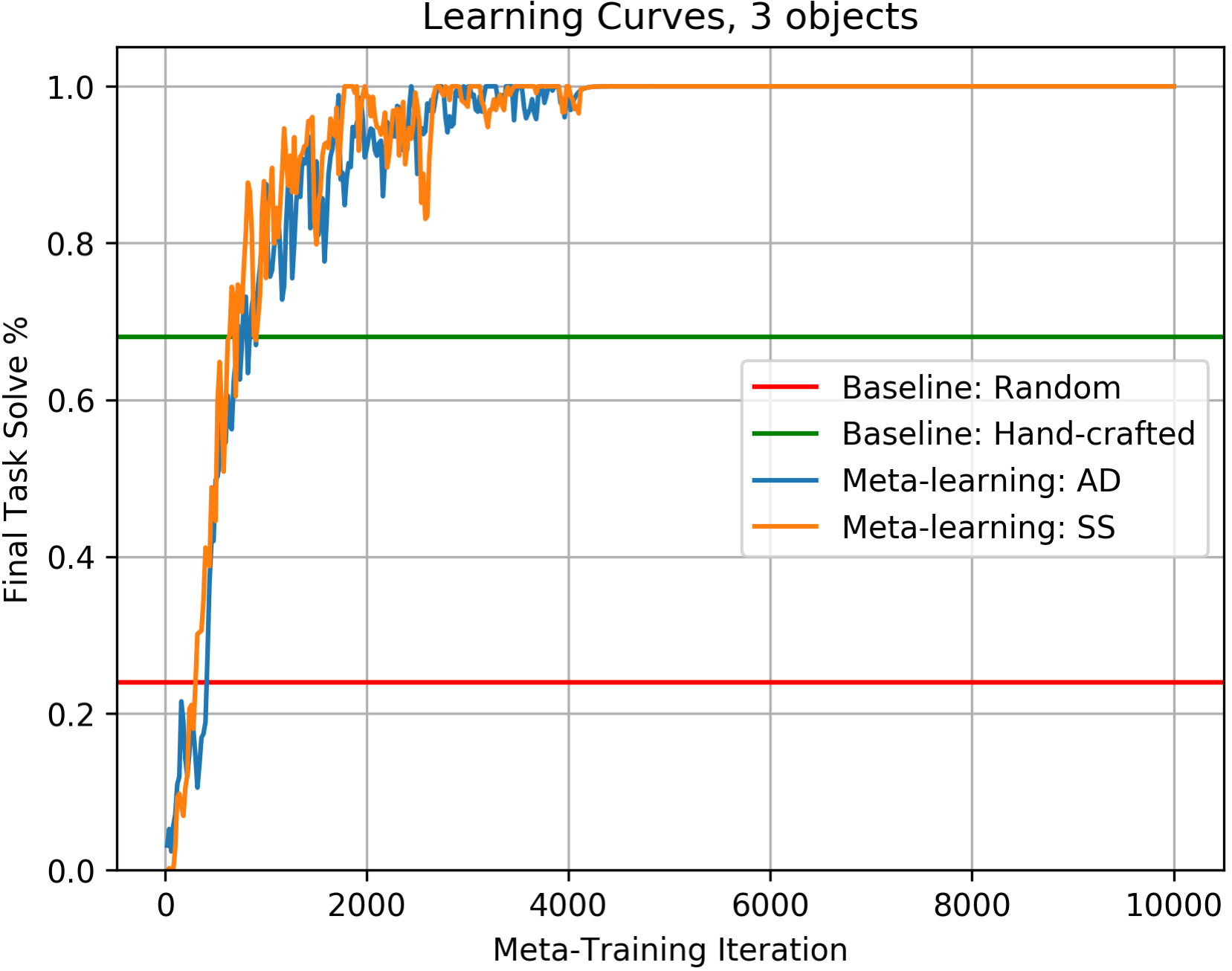
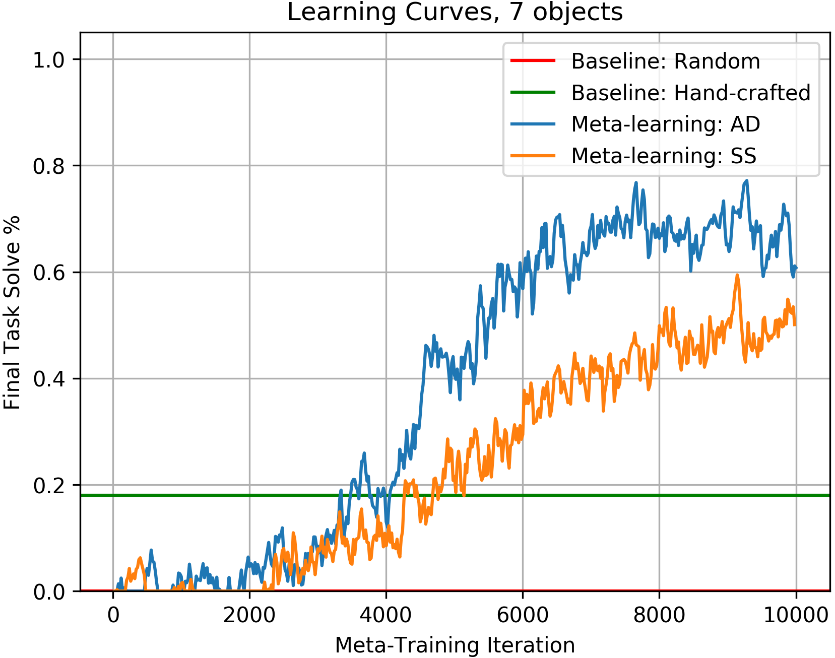
Figure 2: Learning curves over $10^{4}$ training iterations (smoothed).

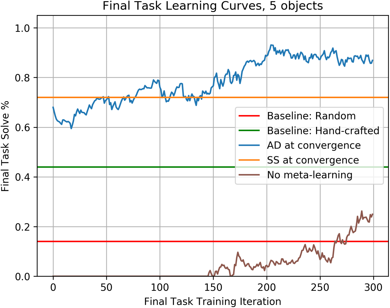
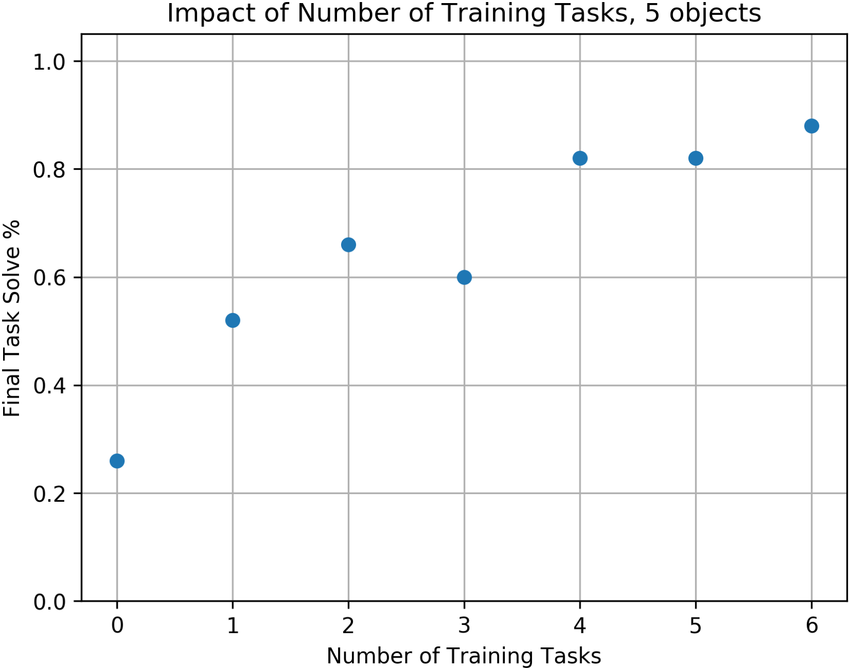
Figure 3: Left: Final task learning curves (smoothed), showing that learning to do the evaluation tasks is much more efficient when starting from meta-trained specializers (blue, orange) versus a randomly initialized ad learner (brown). Right: To investigate the importance of having a diversity of training tasks, we ran the ad learner while withholding some training tasks out of our full suite of 6. We can see that the final task performance (across all 3 evaluation tasks) improves when the agent is trained across more tasks.

VI Conclusion and Future Work

We used modular meta-learning to address the problem of learning continuous action parameters in multi-task tamp.

One interesting avenue for future work is to allow the specializers to be functions of the full plan skeleton, which would provide them with context necessary for picking good parameter values in more complex domains. Another is to remove the assumption of deterministic specializers by having them either be stochastic neural networks or output a distribution over the next state, reparameterized using Gumbel-Softmax [22]. Finally, we hope to explore tasks requiring planning under uncertainty. These tasks would require more sophisticated compositional structures; we would need to search over tree-structured policies, rather than sequential plans as in this work. This search could be made tractable using heuristics for solving pomdps [23, 24, 25].

References

- [1] L. P. Kaelbling and T. Lozano-Pérez, “Hierarchical task and motion planning in the now,” in Robotics and Automation (ICRA), 2011 IEEE International Conference on. IEEE, 2011, pp. 1470–1477.
- [2] S. Srivastava, E. Fang, L. Riano, R. Chitnis, S. Russell, and P. Abbeel, “Combined task and motion planning through an extensible planner-independent interface layer,” in Robotics and Automation (ICRA), 2014 IEEE International Conference on. IEEE, 2014, pp. 639–646.
- [3] C. Finn, P. Abbeel, and S. Levine, “Model-agnostic meta-learning for fast adaptation of deep networks,” arXiv preprint arXiv:1703.03400, 2017.
- [4] F. Alet, T. Lozano-Pérez, and L. P. Kaelbling, “Modular meta-learning,” arXiv preprint arXiv:1806.10166 (to appear in CoRL 18), 2018.
- [5] J. Peters, J. Kober, K. Mülling, O. Krämer, and G. Neumann, “Towards robot skill learning: From simple skills to table tennis,” in Joint European Conference on Machine Learning and Knowledge Discovery in Databases, 2013, pp. 627–631.
- [6] J. Kober, J. A. Bagnell, and J. Peters, “Reinforcement learning in robotics: A survey,” The International Journal of Robotics Research, vol. 32, no. 11, pp. 1238–1274, 2013.
- [7] B. Argall and A. Billard, “A survey of tactile human-robot interactions,” Robotics and Autonomous Systems, vol. 58, no. 10, pp. 1159–1176, 2010.
- [8] H. Pasula, L. S. Zettlemoyer, and L. P. Kaelbling, “Learning symbolic models of stochastic domains,” J. Artif. Intell. Res. (JAIR), vol. 29, 2007.
- [9] B. Kim, L. P. Kaelbling, and T. Lozano-Pérez, “Learning to guide task and motion planning using score-space representation,” in Robotics and Automation (ICRA), 2017 IEEE International Conference on. IEEE, 2017, pp. 2810–2817.
- [10] ——, “Guiding search in continuous state-action spaces by learning an action sampler from off-target search experience,” in Proceedings of Thirty-Second AAAI Conference on Artificial Intelligence, 2018.
- [11] Z. Wang, C. R. Garrett, L. P. Kaelbling, and T. Lozano-Pérez, “Active model learning and diverse action sampling for task and motion planning,” arXiv preprint arXiv:1803.00967, 2018.
- [12] R. Chitnis, D. Hadfield-Menell, A. Gupta, S. Srivastava, E. Groshev, C. Lin, and P. Abbeel, “Guided search for task and motion plans using learned heuristics,” in Robotics and Automation (ICRA), 2016 IEEE International Conference on. IEEE, 2016, pp. 447–454.
- [13] S. J. Pan, Q. Yang et al., “A survey on transfer learning,” IEEE Transactions on knowledge and data engineering, vol. 22, no. 10, pp. 1345–1359, 2010.
- [14] J. Andreas, M. Rohrbach, T. Darrell, and D. Klein, “Neural module networks,” in Proceedings of the IEEE Conference on Computer Vision and Pattern Recognition, 2016, pp. 39–48.
- [15] J. Andreas, D. Klein, and S. Levine, “Modular multitask reinforcement learning with policy sketches,” arXiv preprint arXiv:1611.01796, 2016.
- [16] C. R. Garrett, T. Lozano-Pérez, and L. P. Kaelbling, “Sampling-based methods for factored task and motion planning,” arXiv preprint arXiv:1801.00680 (to appear in IJRR), 2018.
- [17] M. Toussaint, “Logic-geometric programming: An optimization-based approach to combined task and motion planning,” in IJCAI, 2015, pp. 1930–1936.
- [18] D. P. Kingma and J. Ba, “Adam: A method for stochastic optimization,” arXiv preprint arXiv:1412.6980, 2014.
- [19] J. J. Kuffner and S. M. LaValle, “RRT-connect: An efficient approach to single-query path planning,” in Robotics and Automation, 2000. Proceedings. ICRA’00. IEEE International Conference on, vol. 2. IEEE, 2000, pp. 995–1001.
- [20] J. Hoffmann and B. Nebel, “The FF planning system: Fast plan generation through heuristic search,” Journal of Artificial Intelligence Research, vol. 14, pp. 253–302, 2001.
- [21] E. Coumans, Y. Bai, and J. Hsu, “Pybullet physics engine,” 2018. [Online]. Available: http://pybullet.org/
- [22] E. Jang, S. Gu, and B. Poole, “Categorical reparameterization with Gumbel-Softmax,” arXiv preprint arXiv:1611.01144, 2016.
- [23] H. Kurniawati, D. Hsu, and W. S. Lee, “SARSOP: Efficient point-based POMDP planning by approximating optimally reachable belief spaces,” in Robotics: Science and systems, vol. 2008. Zurich, Switzerland., 2008.
- [24] J. Pineau, G. Gordon, S. Thrun et al., “Point-based value iteration: An anytime algorithm for POMDPs,” in IJCAI, vol. 3, 2003, pp. 1025–1032.
- [25] A. Somani, N. Ye, D. Hsu, and W. S. Lee, “DESPOT: Online POMDP planning with regularization,” in Advances in neural information processing systems, 2013, pp. 1772–1780.