Lepto-philic 2-HDM + singlet scalar portal induced fermionic dark matter

Abstract

We explore the possibility that the discrepancy in the observed anomalous magnetic moment of the muon $\Delta a_{\mu}$ and the predicted relic abundance of Dark Matter by Planck data, can be explained in a lepto-philic 2-HDM augmented by a real SM singlet scalar of mass $\sim$ 10-80 GeV. We constrain the model from the observed Higgs Decay width at LHC, LEP searches for low mass exotic scalars and anomalous magnetic moment of an electron $\Delta a_{e}$. This constrained light singlet scalar serves as a portal for the fermionic Dark Matter, which contributes to the required relic density of the universe. A large region of model parameter space is found to be consistent with the present observations from the Direct and Indirect DM detection experiments.

1 Introduction

Investigations into the nature of dark matter (DM) particles and their interactions is an important field of research in Astro-particle physics. The Atlas and CMS collaborations at the Large Hadron Collider (LHC) are searching for the signature of DM particles involving missing energy ($\not\!\!\!E_{T}$) Garny:2013ama ; GooDMan:2010yf accompanied by a single or two jet events. Direct detection experiments measure the nuclear-recoil energy and its spectrum in DM-Nucleon elastic scattering Hisano:2011um ; Garny:2012eb . In addition, there are Indirect detection experiment Ackermann:2013yva searching for the DM annihilation into photons and neutrinos in cosmic rays. These experiments have now reached a level of sensitivity where a significant part of parameter space required for the observed relic density, if contributed by the dark matter composed of Weakly interacting massive particles (WIMPs) that survive as thermal relics, has been excluded. The null results of these direct and indirect experiments have given rise to the consideration of ideas where the dark matter is restricted to couple exclusively to either Standard Model (SM) leptons (lepto-philic) or only to top quarks (top-philic). In these scenarios the DM-Nucleon scattering occurs only at the loop level and the constraints from direct detection are weaker.

Extended Higgs sector have been studied in literature Dedes:2001nx ; Abe:2015oca ; Chun:2015hsa to explain discrepancy in anomalous magnetic moment of muon. Recently a simplified Dark Higgs portal model of the order of $\lesssim$ few GeV, that couples predominantly to leptons with the coupling constant $\sim\,m_{l}/v_{o}$ where $m_{l}$ is the lepton mass and $v_{o}$ is the Higgs VEV, has been considered in the literature Chen:2015vqy . This model induces large contribution to the anomalous magnetic moment of muon and can explain the existing discrepancy between the experimental observation $a^{\rm exp}_{\mu}=$ 11 659 209.1(5.4)(3.3)$\times 10^{-10}$ pdg2018-muon and theoretical prediction $a^{\rm SM}_{\mu}=$ 116 591 823(1)(34)(26) $\times 10^{-11}$ Hagiwara:2011af ; pdg2018-muon of the muon anomalous magnetic moment $\Delta a_{\mu}\equiv a_{\mu^{-}}^{\rm exp}-a_{\mu^{-}}^{\text{SM}}\,=\,268(63)\,\times 10^{-11}$ pdg2018-muon without compromising the experimental measurement of electron anomalous magnetic moment $a^{\rm exp}_{e}=(1159.65218091\pm 0.00000026)\times 10^{-6}$ pdg2018-electron . It has been shown in the literature Batell:2016ove , that with the inclusion of an additional singlet scalar below the electro-weak scale to the lepto-philic 2-HDM makes the model UV complete. This UV complete model with an extra singlet scalar $\sim\,\,<$ 10 GeV successfully explains the existing 3 $\sigma$ discrepancy of muon anomalous magnetic moment and is consistent with the constraints on the model parameters from muon and meson decays Bird:2004ts ; OConnell:2006rsp ; Batell:2009jf ; Krnjaic:2015mbs . These results have been analysed for 0.01 GeV < $m_{S^{0}}$ < 10 GeV when compared with those for the singlet neutral vector $Z^{\prime}$ searches at $B$ factories such as BaBar TheBABAR:2016rlg , from electron beam dump experiments Battaglieri:2014hga and electroweak precision experiments Lebedev:2000ix etc.

In reference Agrawal:2014ufa , the authors have explored the possibility of explaining the anomalous magnetic moment of muon with an additional lepto-philic light scalar mediator assuming the universal coupling of the scalar with all leptons constrained from the LEP Schael:2013ita resonant production and the BaBar experiments TheBABAR:2016rlg . These constraints were found to exclude all of the scalar mediator mass range except between 10 MeV and 300 MeV.

In the current paper we consider fermionic dark matter that couples predominately with SM leptons through the non-universal couplings with the scalar portal in the UV complete lepto-philic 2-HDM model. We relax the requirement of the very light scalar considered in Batell:2016ove and investigate parameter space for a comparatively heavier scalar 10 GeV $\lesssim\,m_{S^{0}}\,\lesssim$ 80 GeV. In section 2, we give a brief review of this simplified model, using the full Lagrangian and couplings of the Singlet scalar $S^{0}$ with all model particles. In section 3, we calculate the contribution from scalars ($S^{0},H^{0},A^{0},H^{\pm}$) to the anomalous magnetic moment of the muon and discuss bounds on the model parameters from LEP-II, $\Delta a_{e}$ and upper bound on the observed total Higgs decay width. Implications of the model contributions to the lepton couplings non-universality and the oblique corrections are briefly discussed along-with available constraints on them.

In the present study we are motivated to explore the possibility of simultaneously explaining the discrepancy in the observed anomalous magnetic moment of the muon on the one hand and the expected relic density contribution from DM on the other. Accordingly, in section 4, we introduce the DM contributing to the relic density through dark matter - SM particles interactions induced by the additional scalar in the model and scan for the allowed parameter space which is consistent with direct and indirect experimental data as well as with the observed value of the $\Delta a_{\mu}$. Section 5 is devoted to discussion and summary of results.

2 The Model

We consider a UV complete lepton specific 2-HDM with a singlet scalar portal interacting with the fermionic DM. In this model the two Higgs doublets $\Phi_{1}$ and $\Phi_{2}$ are so arranged that $\Phi_{1}$ couples exclusively to leptons while $\Phi_{2}$ couples exclusively to quarks. The ratio of their VEV’s $\left\langle\Phi_{1}\right\rangle/\,\left\langle\Phi_{2}\right\rangle\equiv\,v_{2}/\,v_{1}$ = $\tan\beta$ is assumed to be large. In this model the scalars (other than that identified with the CP even $h^{0}\,\sim$ 125 GeV) couple to leptons and quarks with coupling enhanced and suppressed by $\tan\beta$ respectively. A mixing term in the potential $A_{12}\,\left[\Phi_{1}^{\dagger}\Phi_{2}+\Phi_{2}^{\dagger}\Phi_{1}\right]\,\varphi^{0}$ results in the physical scalar $S^{0}$ coupling to leptons with strength proportional to $m_{l}/v_{o}$ where

$$v_{o}\equiv\sqrt{v_{1}^{2}+v_{2}^{2}}\,=\,246\,{\rm GeV}.$$ (1)

The full scalar potential is given by

$$V(\Phi_{1},\Phi_{2},\varphi^{0})=V_{2-HDM}+V_{\varphi^{0}}+V_{\rm portal}$$ (2)

where CP conserving $V_{2-HDM}$ is given as

$$V_{2-HDM}(\Phi_{1},\Phi_{2}) = m^{2}_{11}\,\Phi_{1}^{\dagger}\Phi_{1}+m^{2}_{22}\,\Phi_{2}^{\dagger}\Phi_{2}-\left(m^{2}_{12}\,\Phi_{1}^{\dagger}\Phi_{2}+{\rm h.c.}\right)+\frac{\lambda_{1}}{2}\,\left(\Phi_{1}^{\dagger}\Phi_{1}\right)^{2}+\frac{\lambda_{2}}{2}\,\left(\Phi_{2}^{\dagger}\Phi_{2}\right)^{2}$$ (3)

$$+\lambda_{3}\,\left(\Phi_{1}^{\dagger}\Phi_{1}\right)\left(\Phi_{2}^{\dagger}\Phi_{2}\right)+\lambda_{4}\,\left(\Phi_{1}^{\dagger}\Phi_{2}\right)\left(\Phi_{2}^{\dagger}\Phi_{1}\right)+\left\{\frac{\lambda_{5}}{2}\,\left(\Phi_{1}^{\dagger}\Phi_{2}\right)^{2}+{\rm h.c.}\right\}\,$$

and $V_{\varphi^{0}}$ and $V_{\rm portal}$ is assumed to be

$$V_{\varphi^{0}} = B\varphi^{0}+\frac{1}{2}m_{0}^{2}(\varphi^{0})^{2}+\frac{A_{\varphi^{0}}}{2}(\varphi^{0})^{3}+\frac{\lambda_{\varphi^{0}}}{4}(\varphi^{0})^{4}.$$ (4)

$$V_{\rm portal} = A_{11}\,\left(\Phi_{1}^{\dagger}\Phi_{1}\right)\,\varphi^{0}+A_{12}\,\left(\Phi_{1}^{\dagger}\Phi_{2}+\Phi_{2}^{\dagger}\Phi_{1}\right)\,\varphi^{0}+A_{22}\,\left(\Phi_{2}^{\dagger}\Phi_{2}\right)\,\varphi^{0}.$$ (5)

where the scalar doublets

$$\Phi_{1}=\frac{1}{\sqrt{2}}\begin{pmatrix}\sqrt{2}\omega_{1}^{+}\\ \rho_{1}+v_{o}\,\cos\beta+i\,z_{1}\end{pmatrix};\,\,\,\,\,\Phi_{2}=\frac{1}{\sqrt{2}}\begin{pmatrix}\sqrt{2}\omega_{2}^{+}\\ \rho_{2}+v_{o}\,\sin\beta+i\,z_{2}\end{pmatrix}\,.$$ (6)

are written in terms of the mass eigenstates $G^{0}$, $A^{0}$ , $G^{\pm}$ and $H^{\mp}$ as

$$\begin{pmatrix}z_{1}\\ z_{2}\end{pmatrix}=\left(\begin{array}[]{ccc}\cos\beta&&-\sin\beta\\ \sin\beta&&\cos\beta\end{array}\right)\begin{pmatrix}G^{0}\\ A^{0}\end{pmatrix}; \,\,\,\begin{pmatrix}\omega_{1}\\ \omega_{2}\end{pmatrix}=\left(\begin{array}[]{ccc}\cos\beta&&-\sin\beta\\ \sin\beta&&\cos\beta\end{array}\right)\begin{pmatrix}G^{\pm}\\ H^{\pm}\end{pmatrix}.$$ (11)

Here $G^{0}$ & $G^{\pm}$ are Nambu-Goldstone Bosons absorbed by the $Z^{0}$ and W^± vector Bosons, $A^{0}$ is the pseudo-scalar and $H^{\pm}$ are the charged Higgs. The three CP even neutral scalar mass eigen-states mix among themselves under small mixing angle approximations

$$\sin\delta_{13}\sim\delta_{13}\simeq-\frac{v_{0}\,A_{12}}{m_{H^{0}}^{2}},\,\,{\rm and}\,\,\sin\delta_{23}\sim\delta_{23}\simeq-\frac{v_{0}\,A_{12}}{m_{h^{0}}^{2}}\left[1+\xi^{h^{0}}_{\ell}\left(1-\frac{m_{h^{0}}^{2}}{m_{H^{0}}^{2}}\right)\right]\cot\beta$$ (13)

to give three CP even neutral weak eigen-states as

$$\left(\begin{array}[]{c}\rho_{1}\\ \rho_{2}\\ \varphi^{0}\end{array}\right)\simeq\left(\begin{array}[]{ccccc}-\sin\alpha&&\cos\alpha&&\delta_{13}\\ \,\,\,\cos\alpha&&\sin\alpha&&\delta_{23}\\ \delta_{13}\sin\alpha-\delta_{23}\cos\alpha&&\,\,-\delta_{13}\cos\alpha-\delta_{23}\sin\alpha&&1\end{array}\right)\left(\begin{array}[]{c}h^{0}\\ H^{0}\\ S^{0}\end{array}\right);$$ (23)

The mixing matrix given in equation (23) validates the orthogonality condition up to an order $\lesssim\,\mathcal{O}\left(\delta_{13}^{2},\delta_{23}^{2},\delta_{13}\delta_{23}\right)$. $\xi_{l}^{h^{0}}$ is chosen to be $\sim$ 1 in the alignment i.e. ($\beta-\alpha$) $\simeq\pi/2$.

The spectrum of the model at the electro-weak scale is dominated by $V_{2-HDM}$. The $V_{\varphi^{0}}$ and $V_{\rm portal}$ interactions are treated as perturbations. After diagonalization of the scalar mass matrix, the masses of the physical neutral scalars are given by

$$m_{S^{0}}^{2} \simeq m_{0}^{2}+2\delta_{13}\,M_{13}^{2}+2\delta_{23}\,M_{23}^{2}$$ (24)

$$m_{h^{0},\,H^{0}}^{2} \simeq \frac{1}{2}\left[M_{11}^{2}+M_{22}^{2}\mp\sqrt{\left(M_{11}^{2}-M_{22}^{2}\right)^{2}+4\,M_{12}^{4}}\right]$$ (25)

where

$$M_{11}^{2}=m_{12}^{2}\tan\beta+\lambda_{1}v_{0}^{2}\cos^{2}\beta; M_{12}^{2}=-\,m_{12}^{2}+\left(\lambda_{3}+\lambda_{4}+\lambda_{5}\right)v_{0}^{2}\cos\beta\,\sin\beta;$$

$$M_{22}^{2}=m_{22}^{2}\cot\beta+\lambda_{2}v_{0}^{2}\sin^{2}\beta; M_{13}^{2}=v_{0}\,A_{12}\,\sin\beta;\,\,\,M_{23}^{2}=v_{0}\,A_{12}\,\cos\beta;$$ (26)

In the alignment limit, one of the neutral CP even scalar $h^{0}$ $\approx$ 125 GeV is identified with the SM Higgs.

The coefficients $m_{0}^{2}$, $m_{11}^{2},\,m_{22}^{2}$ and $\lambda_{i}$ for $i=1,\cdot\cdot\cdot,5$ are explicitly defined in terms of the physical scalar masses, mixing angles $\alpha$ and $\beta$ and the free parameter $m_{12}^{2}$ and are given in the Appendix A. Terms associated with $A_{11}$ are proportional to $\cot\beta$ and therefore can be neglected as they are highly suppressed in the large $\tan\beta$ limit. Terms proportional to $A_{22}$ are tightly constrained from the existing data at LHC on decay of a heavy exotic scalar to di-higgs channel and therefore they are dropped. The coefficient $B$ is fixed by redefinition of the field $\varphi^{0}$ to avoid a non-zero VEV for itself.

$\xi^{\phi}_{\psi}$/$\xi^{\phi}_{V}$	$S^{0}$	$h^{0}$	$H^{0}$	$A^{0}$	$H^{\pm}$
$\ell$	$\delta_{13}/c_{\beta}$	$-s_{\alpha}/c_{\beta}$	$c_{\alpha}/c_{\beta}$	$-s_{\beta}/c_{\beta}$	$-s_{\beta}/c_{\beta}$
$u_{q}$	$\delta_{23}/s_{\beta}$	$c_{\alpha}/s_{\beta}$	$s_{\alpha}/s_{\beta}$	$c_{\beta}/s_{\beta}$	$c_{\beta}/s_{\beta}$
$d_{q}$	$\delta_{23}/s_{\beta}$	$c_{\alpha}/s_{\beta}$	$s_{\alpha}/s_{\beta}$	$-c_{\beta}/s_{\beta}$	$c_{\beta}/s_{\beta}$
$Z^{0}$/$W^{\pm}$	$\delta_{13}c_{\beta}+\delta_{23}s_{\beta}$	$s_{\left(\beta-\alpha\right)}$	$c_{\left(\beta-\alpha\right)}$	-	-

Table 1: Values of $\xi^{\phi}_{\psi}$ and $\xi^{\phi}_{V}$ for $\phi=S^{0}$, $h^{0}$, $H^{0}$, $A^{0}$ and $H^{\pm}$; $\psi=\ell$, $u_{q}$ and $d_{q}$; $V$= $W^{\pm}$ and $Z^{0}$ in the lepto-philic 2-HDM+$S^{0}$ model. These values coincide with couplings given in reference Batell:2016ove in the alignment limit i.e. ($\beta-\alpha$) $\simeq\pi/2$. In the table $s$ and $c$ stands for $\sin$ and $\cos$ respectively.

The Yukawa couplings arising due to Higgs Doublets $\Phi_{1}$ and $\Phi_{2}$ in type-X 2-HDM is given by

$$-{\cal L}_{Y}=\bar{L}Y_{e}\Phi_{1}e_{R}+\bar{Q}Y_{d}\Phi_{2}d_{R}+\bar{Q}Y_{u}\tilde{\Phi}_{2}u_{R}+{\rm h.c.},$$ (27)

$$m_{e}=\cos\beta\times\frac{Y_{e}v_{o}}{\sqrt{2}},~{}~{}m_{u(d)}=\sin\beta\times\frac{Y_{u(d)}v_{o}}{\sqrt{2}}.$$ (28)

We re-write the Yukawa interactions of the physical neutral states as

$$-{\cal L}_{Y} \supset\sum_{\phi\equiv S^{0},h^{0},H^{0}}\,\,\sum_{\psi=\ell,\,q}\xi^{\phi}_{\psi}\,\frac{m_{\psi}}{v_{o}}\,\,\phi\,\,\bar{\psi}\psi$$ (29)

The couplings $\xi_{\psi}^{\phi}$ are given in the first three rows of table 1. It is important to mention here that the Yukawa couplings are proportional to the fermion mass i.e. non-universal unlike the consideration in reference Agrawal:2014ufa .

The interaction of the neutral scalar mass eigenstates with the weak gauge Bosons are given by

$${\cal L} \supset\sum_{\phi\equiv S^{0},h^{0},H^{0}}\,\frac{\phi}{v_{o}}\,\,\left(2\,\,\xi^{\phi}_{W^{\pm}}\,\,m^{2}_{W^{\pm}}\,W^{+}_{\mu}{W^{-}}^{\mu}+\xi^{\phi}_{Z^{0}}\,\,\,\,m_{Z^{0}}^{2}\,{Z^{0}}_{\mu}{Z^{0}}^{\mu}\right).$$ (30)

The couplings $\xi_{V}^{\phi}$ are given in the last row of table 1. It is to be noted that for $m_{H^{0}}>>m_{h^{0}}$, the singlet scalar coupling with $Z^{0}$ Boson can be fairly approximated as $\simeq\delta_{23}\sin\beta$.

The recent precision measurements at LHC constrains $\left|\kappa_{V}\right|$ = 1.06${}^{+0.10}_{-0.10}$ Aad:2015ona ; pdg2018Higgs (where $\kappa_{V}$ is the scale factor for the SM Higgs Boson coupling) to the vector Bosons restricts the generic 2HDM Models and its extension like the one in discussion to comply with the alignment limit. In this model, the Higgs Vector Boson coupling to gauge Bosons is identical to that of generic 2HDM model at tree level as the additional singlet scalar contributes to $h^{0}VV$ couplings only at the one loop level which is suppressed by $\delta^{2}_{23}/\left(16\,\pi^{2}\right)$.

The triple scalar couplings of the mass eigen states are given in the Appendix D, some of which can be constrained from the observed Higgs decay width and exotic scalar Boson searches at LEP, TeVatron and LHC.

3 Electro-Weak Constraints

3.1 Anomalous Magnetic Moment of Muon

We begin our analysis by evaluating the parameter space allowed from 3 $\sigma$ discrepancy $a_{\mu^{-}}^{\rm exp}-a_{\mu^{-}}^{\text{SM}}\,\equiv\Delta a_{\mu}=\,268(63)\,\times 10^{-11}$ pdg2018-muon . In lepto-philic 2-HDM + singlet scalar portal model all five additional scalars $S^{0},\,H^{0},\,A^{0},\,H^{\pm}$ couple to leptons with the coupling strengths given in table 1 and thus give contributions to $\Delta a_{\mu}$ at the one-loop level and are expressed as:

$$\Delta a_{\mu} = \Delta a_{\mu}\arrowvert_{S^{0}}+\Delta a_{\mu}\arrowvert_{H^{0}}+\Delta a_{\mu}\arrowvert_{A^{0}}+\Delta a_{\mu}\arrowvert_{H^{\pm}}$$ (31)

$$= \frac{1}{8\pi^{2}}\frac{m^{2}_{\mu}}{v_{o}^{2}}\,\tan^{2}\beta\left[\delta_{13}^{2}\,\,I_{S^{0}}+I_{H^{0}}+I_{A^{0}}+\,I_{H^{\pm}}\right].$$

Here $I_{i}$ are the integrals given as

$$I_{S^{0},\,H^{0}}=\int^{1}_{0}dz\frac{\left(1+z\right)\left(1-z\right)^{2}}{\left(1-z\right)^{2}+z\,r_{{S^{0}},\,H^{0}}^{-2}};\,\,\, I_{A^{0}}=-\,\int^{1}_{0}dz\frac{z^{3}}{r_{A^{0}}^{-2}\left(1-z\right)+z^{2}};\,\,\,{\rm and}$$

$$I_{H^{\pm}}=\int^{1}_{0}dz\frac{z(1-z)}{\left(1-z\right)-r_{H^{\pm}}^{-2}}\,\,\, {\rm with}\,\,\,r_{i}\equiv\frac{m_{l}}{m_{i}}\,\,{\rm for}\,\,i\equiv S^{0},\,H^{0},\,A^{0},\,H^{\pm}.$$ (32)

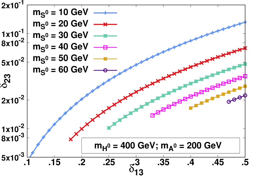
(a)

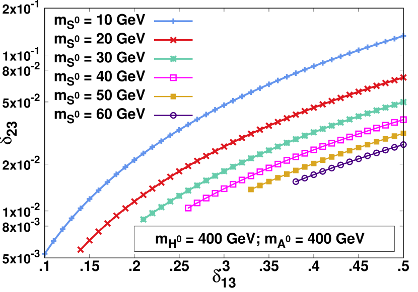
(b)

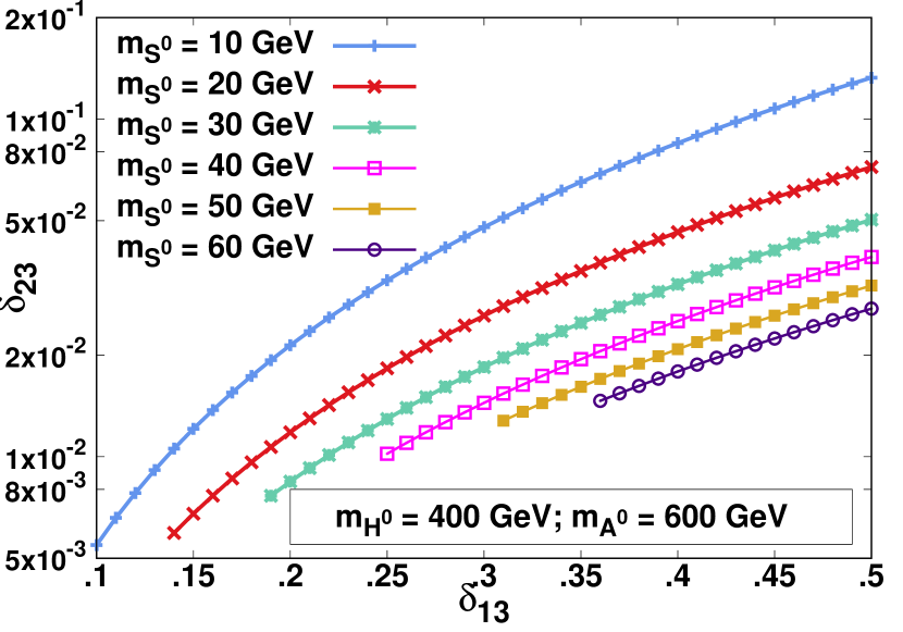
(c)

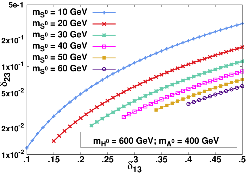
(d)

Figure 1: Figures 1(a), 1(b), 1(c) and 1(d) show contours on the $\delta_{13}$ - $\delta_{23}$ plane satisfying $\Delta a_{\mu}=\,268(63)\,\times 10^{-11}$ corresponding to four different combinations of $m_{H^{0}}$ and $m_{A^{0}}$ respectively. In each panel six contours are depicted corresponding to six choices of singlet masses 10, 20, 30, 40, 50 and 60 GeV respectively.

We observe that in the limit $r_{i}<<1$ the charged scalar integral $I_{H^{\pm}}$ is suppressed by 2-3 orders of magnitude in comparison to the other integrals for the masses of the scalars varying between 150 GeV $\sim$ 1.6 TeV. Since the present lower bound on the charged Higgs mass from its searches at LHC is 600 GeV Aad:2015typ , we can neglect its contribution to the $\Delta a_{\mu}$ in our calculations.

It is also important to note that the one loop contribution from the pseudo-scalar integral $I_{A^{0}}$ is opposite in sign to that of the other neutral scalars $I_{H^{0},\,h^{0},\,S^{0}}$, while at the level of two loops the Barr-Zee diagrams Ilisie:2015tra , it gives positive contribution to $\Delta a_{\mu}$ which may be sizable for low pseudo-scalar mass $m_{A^{0}}$ because of large value of the coupling $\xi^{A^{0}}_{l}$. However, for heavy $A^{0}$ and $H^{0}$ considered here, we can safely neglect the two loop contributions.

In the alignment limit the mixing angle $\delta_{23}\simeq\frac{\delta_{13}m^{2}_{H^{0}}}{m_{h^{0}}^{2}}\left[2-\frac{m_{h^{0}}^{2}}{m_{H^{0}}^{2}}\right]\cot\beta$ is fixed by constrains from $\Delta a_{\mu}$ and choice of $\delta_{13}$ and neutral CP-even scalar masses. To understand the model we study the correlation of the two mixing parameters $\delta_{13}$ and $\delta_{23}$ satisfying the $\Delta a_{\mu}$ for a given set of input masses of the physical scalars and show four correlation plots in figures 1(a), 1(b), 1(c) and 1(d) for varying $\delta_{13}$. We find that $\delta_{23}$ remains small enough for all the parameter space in order to fulfill the small angle approximation. We have chosen six singlet scalar masses 10, 20, 30, 40, 50, and 60 GeV. In each panel $m_{H^{0}}$ and $m_{A^{0}}$ are kept fixed at values, namely (a) $m_{H^{0}}$ = 400 GeV, $m_{A^{0}}$ = 200 GeV, (b) $m_{H^{0}}$ = 400 GeV, $m_{A^{0}}$ = 400 GeV, (c) $m_{H^{0}}$ = 400 GeV, $m_{A^{0}}$ = 600 GeV, and (d) $m_{H^{0}}$ = 600 GeV, $m_{A^{0}}$ = 400 GeV. We find that relatively larger values of $\delta_{13}$ are required with the increase in scalar mass $m_{S^{0}}$. Increase in the pseudo-scalar mass $m_{A^{0}}$ for fixed $m_{H^{0}}$ results in the lower value of $\delta_{13}$ required to obtain the observed $\Delta a_{\mu}$.

On imposing the perturbativity constraints on the Yukawa coupling $\xi^{H^{0}}_{\tau}\equiv\tan\beta\,m_{\tau}/v_{0}$ involving the $\tau^{\pm}$ and $H^{0}$, we compute the upper bound on the model parameter $\tan\beta\lesssim$ 485. As a consequence, we observe that the values of $\delta_{23}$ also gets restricted for each variation curve exhibited in figures 1(a), 1(b), 1(c) and 1(d).

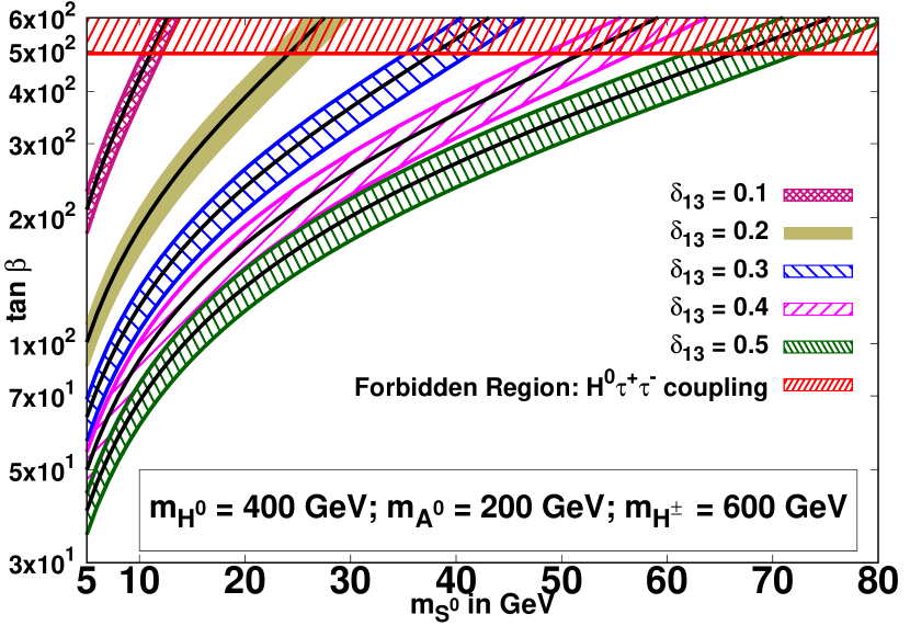
(a)

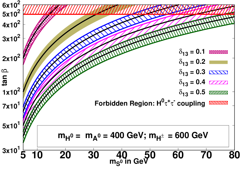
(b)

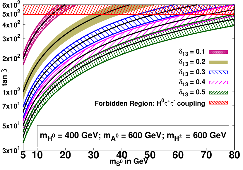
(c)

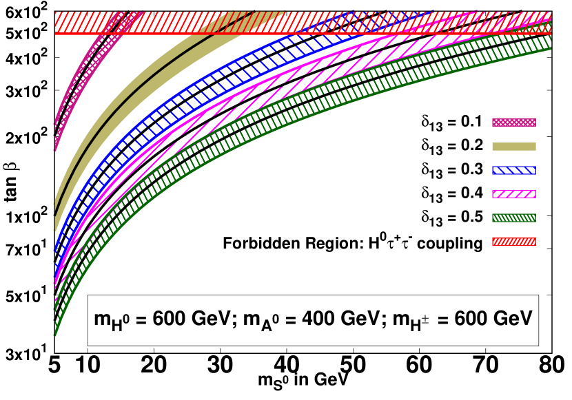
(d)

Figure 2: Figures 2(a), 2(b), 2(c) and 2(d) show contours on $m_{S^{0}}$ - $\tan\beta$ plane satisfying $\Delta a_{\mu}=\,268(63)\,\times 10^{-11}$ for fixed $m_{H^{\pm}}$ = 600 GeV and four different combinations of $m_{H^{0}}$ and $m_{A^{0}}$ as shown. In each panel, five contours along-with shaded one $\sigma$ bands of $\Delta a_{\mu}$ are depicted corresponding to five choices of $\delta_{13}$ 0.1, 0.2, 0.3, 0.4 and 0.5 respectively. The top horizontal band (shaded in red) in each panel shows the forbidden region on $\tan\beta$ due to the perturbativity constraint on the upper limit of $H^{0}\tau^{+}\tau^{-}$ coupling.

The contours satisfying $\Delta a_{\mu}=\,268(63)\,\times 10^{-11}$ on $m_{S^{0}}$ - $\tan\beta$ plane for fixed charged Higgs mass $m_{H^{\pm}}$ = 600 GeV are shown for four different combinations of heavy neutral Higgs mass and pseudo-scalar Higgs mass namely (a) $m_{H^{0}}$ = 400 GeV, $m_{A^{0}}$ = 200 GeV, (b) $m_{H^{0}}$ = 400 GeV, $m_{A^{0}}$ = 400 GeV, (c) $m_{H^{0}}$ = 400 GeV, $m_{A^{0}}$ = 600 GeV, and (d) $m_{H^{0}}$ = 600 GeV, $m_{A^{0}}$ = 400 GeV respectively in figures 2(a), 2(b), 2(c) and 2(d). In each panel the five shaded regions, correspond to five choices of mixing angle $\delta_{13}$ = 0.1, 02, 0.3, 0.4 and 0.5 respectively depict the 3 $\sigma$ allowed regions for the discrepancy in $\Delta a_{\mu}$ around its central value shown by the black lines. The horizontal band appearing at the top in all these panels shows the forbidden region on account of the perturbativity constraint on the upper limit of $H^{0}\tau^{+}\tau^{-}$ coupling as discussed above.

As expected the allowed value of $\tan\beta$ increases with the increasing singlet scalar mass $m_{S^{0}}$ and decreasing mixing angle $\delta_{13}$. We find that a very narrow region of the singlet scalar mass is allowed by $\Delta a_{\mu}$ corresponding to $\delta_{13}\leq 0.1$.

3.2 LEP and $\Delta a_{e}$ Constraints

Searches for the light neutral Bosons were explored in the Higgs associated vector Boson production channels at LEP Abdallah:2004wy . We consider the s-channel bremsstrahlung process $e^{+}e^{-}\rightarrow Z^{0}/\gamma^{0}+h^{0}\rightarrow\tau^{+}\tau^{-}\tau^{+}\tau^{-}$ whose production cross-section can be expressed in terms of the SM $h^{0}Z^{0}$ production cross-section and given as

$$\sigma_{e^{+}e^{-}\to S^{0}Z^{0}\to\tau^{+}\tau^{-}Z^{0}} = \sigma_{e^{+}e^{-}\to h^{0}Z^{0}}^{\rm SM}\times\left|\frac{\xi^{S^{0}}_{Z^{0}}}{\xi^{h^{0}}_{Z^{0}}}\right|^{2}\times{\rm BR}\left(S^{0}\to\tau^{+}\tau^{-}\right)$$ (33)

$$\equiv \sigma_{e^{+}e^{-}\to h^{0}Z^{0}}^{\rm SM}\times\left|\frac{\delta_{13}c_{\beta}+\delta_{23}s_{\beta}}{\sin\left(\beta-\alpha\right)}\right|^{2}\times{\rm BR}\left(S^{0}\to\tau^{+}\tau^{-}\right).$$

Since the BR$\left(S^{0}\to\tau^{+}\tau^{-}\right)\simeq$ 1, we can compute the exclusion limit on the upper bound on $\left|\xi^{S^{0}}_{Z^{0}}\right|\equiv\left|\delta_{13}c_{\beta}+\delta_{23}s_{\beta}\right|$ from the LEP experimental data Abdallah:2004wy , which are shown in table 2 for some chosen values of singlet scalar masses in the alignment limit.

A light neutral Vector mediator ${Z^{\prime}}^{0}$ has also been extensively searched at LEP Schael:2013ita . Vector mediator ${Z^{\prime}}^{0}$ of mass $\leq$ 209 GeV is ruled out for coupling to muons $\gtrsim$ 0.01 Agrawal:2014ufa . Assuming the same production cross-section corresponding to a light scalar mediator, the constraint on vector coupling can be translated to scalar coupling by multiplying a factor of $\sqrt{2}$. For the case of non-universal couplings where the scalar couples to the leptons with the strength proportional to its mass as is the case in our model, a further factor of $\sqrt{\frac{m_{\mu}}{m_{e}}}$ is multiplied. We therefore find the upper limit on the Yukawa coupling for leptons to be $\xi^{S^{0}}_{l}\frac{m_{l}}{v_{0}}\lesssim$ 0.2.

$m_{S^{0}}$(GeV)	12	15	20	25	30	35	40	45	50	55	60	65
$\left|\xi^{S^{0}}_{Z^{0}}\right|\lesssim$	.285	.316	.398	.530	.751	1.132	1.028	.457	.260	.199	.169	.093

Table 2: Upper limits on $\left|\xi^{S^{0}}_{Z^{0}}\right|$ from bremsstrahlung process $e^{+}e^{-}\to S^{0}Z^{0}\to\tau^{+}\tau^{-}\tau^{+}\tau^{-}$ LEP data Abdallah:2004wy

From the constrained parameter space of the model explaining the muon $\Delta a_{\mu}$, we find that the total contribution to anomalous magnetic moment of the electron comes out $\sim 10^{-15}$. This is two order smaller in the magnitude than the error in the measurement of $a_{e}\simeq\pm 2.6\times 10^{-13}$ pdg2018-electron . The present model is thus capable of accounting for the observed experimental discrepancy in the $\Delta a_{\mu}$ without transgressing the allowed $\Delta a_{e}$.

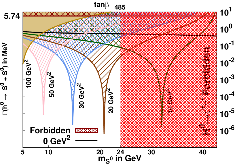
(a) $m_{H^{0}}$ = 400 GeV; $m_{A^{0}}$ = 200 GeV

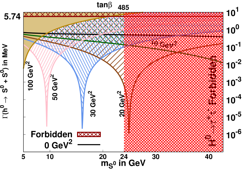
(b) $m_{H^{0}}$ = 400 GeV; $m_{A^{0}}$ = 400 GeV

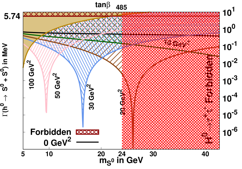
(c) $m_{H^{0}}$ = 400 GeV; $m_{A^{0}}$ = 600 GeV

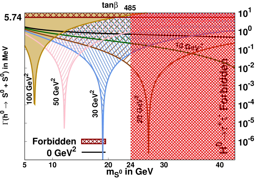
(d) $m_{H^{0}}$ = 600 GeV; $m_{A^{0}}$ = 400 GeV

Figure 3: Figures 3(a), 3(b), 3(c) and 3(d) show $\Gamma_{h^{0}\to S^{0}S^{0}}$ variation with the $m_{S^{0}}$ for $m_{H^{\pm}}$ = 600 GeV, $\delta_{13}$ = 0.2 and four different combinations of $m_{H^{0}}$ and $m_{A^{0}}$ respectively. In each panel we shade five regions corresponding to $m_{12}^{2}$ = 10, 20, 30, 50, 100 GeV² respectively. All points on the solid curves satisfy the discrepancy $\Delta a_{\mu}=\,268(63)\,\times 10^{-11}$ and their corresponding values of $\tan\beta$ are shown in the upper x-axis of all the panels. We plot the contour corresponding to $m_{12}^{2}$ = 0 GeV² in black. The top horizontal band is forbidden from the measurement of the total Higgs decay width at LHC. The red shaded region at the right in each panel is forbidden due to non-perturbativity of $H^{0}\tau^{+}\tau^{-}$ coupling.

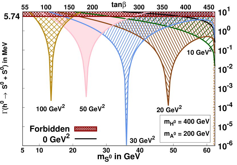
(a)

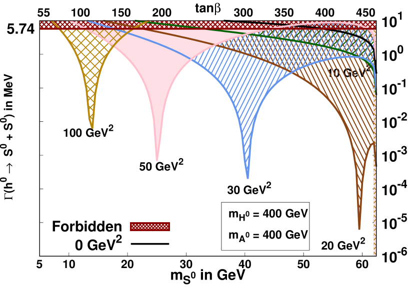
(b)

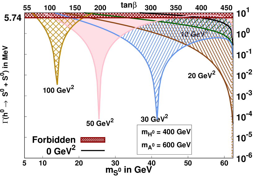
(c)

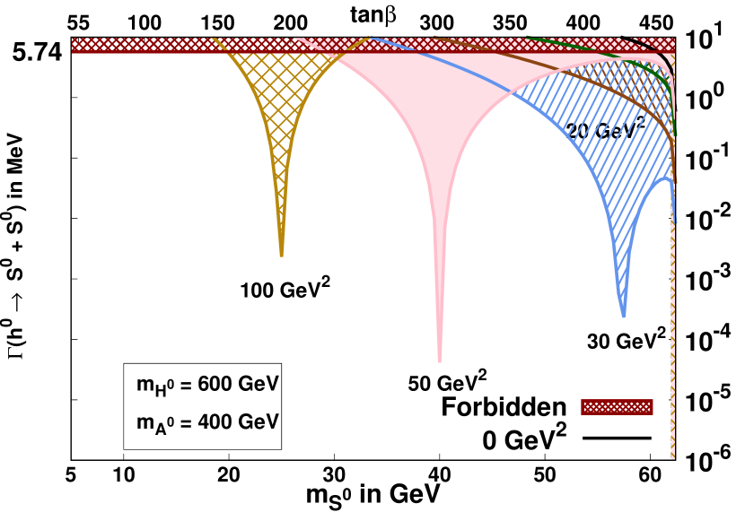
(d)

Figure 4: Figures 4(a), 4(b), 4(c) and 4(d) show $\Gamma_{h^{0}\to S^{0}S^{0}}$ variation with the $m_{S^{0}}$ for $m_{H^{\pm}}$ = 600 GeV, $\delta_{13}$ = 0.4 and four different combinations of $m_{H^{0}}$ and $m_{A^{0}}$ respectively. In each panel we shade five regions corresponding to $m_{12}^{2}$ = 10, 20, 30, 50, 100 GeV² respectively. All points on the solid curves satisfy the discrepancy $\Delta a_{\mu}=\,268(63)\,\times 10^{-11}$ and their corresponding values of $\tan\beta$ are shown in the upper x-axis of all the panels. We plot the contour corresponding to $m_{12}^{2}$ = 0 GeV² in black. The top horizontal band is forbidden from the measurement of the total Higgs decay width at LHC.

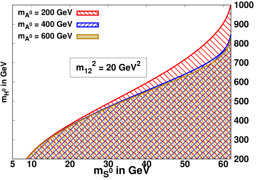
(a)

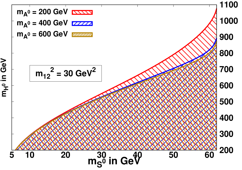
(b)

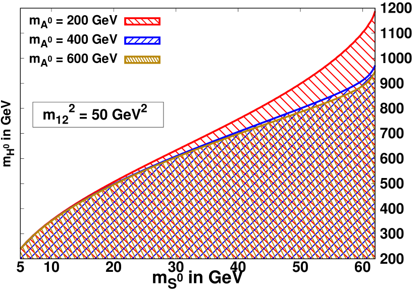
(c)

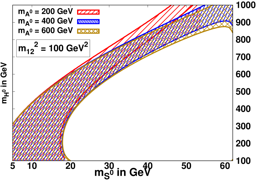
(d)

Figure 5: Figures 5(a), 5(b), 5(c) and 5(d) show contours on the $m_{S^{0}}$ - $m_{H^{0}}$ plane satisfying the 95 % C.L. upper limit on the total observed Higgs decay width $\Gamma_{\rm obs.}^{h^{0}}\leq 2.4\times\Gamma_{\rm SM}^{h^{0}}$ for fixed $m_{H^{\pm}}$ = 600 GeV, $\delta_{13}$ = 0.4 and four different choices of $m_{12}^{2}$ = 20, 30, 50 and 100 GeV². All points on the contours satisfy the discrepancy $\Delta a_{\mu}=\,268(63)\,\times 10^{-11}$. Each panel has three contours corresponding to $m_{A^{0}}$ = 200, 400 and 600 GeV respectively.

3.3 Constraints from Higgs decay-width

Recently CMS analysed the partial decay widths of the off-shell Higgs Boson produced through gluon fusion decaying to $W^{+}W^{-}$ Bosons Khachatryan:2016ctc and then combined the analysis with that for $Z\,Z$ Khachatryan:2015mma vector Bosons to obtain 95 % C.L. upper limit on the total observed Higgs decay width of $2.4\times\Gamma_{\rm SM}^{h^{0}}$ pdg2018Higgs ; Khachatryan:2016ctc , where $\Gamma_{\rm SM}^{h^{0}}\simeq$ 4.1 MeV. The authors have also investigated these decay channels for an off-shell Higgs Boson produced from the vector Boson fusion channels and obtained the upper bound on the total observed Higgs decay width of $19.3\times\Gamma_{\rm SM}^{h^{0}}$ pdg2018Higgs ; Khachatryan:2016ctc . ATLAS also analysed the Higgs decay width assuming that there are no anomalous couplings of the Higgs boson to vector Bosons, and obtained 95% CL observed upper limit on the total width of $6.7\times\Gamma_{\rm SM}^{h^{0}}$ Aad:2015xua . However, we have used the conservative upper limit on the total observed decay width of Higgs Boson of $2.4\times\Gamma_{\rm SM}^{h^{0}}$ for rest of the analysis in our study.

However, in the present model, the scalar identified with SM Higgs Boson $h^{0}$ is in addition likely to decay into two light singlet scalar portals $h^{0}\to S^{0}\,S^{0}$ for $m_{S^{0}}\leq\frac{m_{h^{0}}}{2}$. The partial decay width $\Gamma_{h^{0}\to S^{0}S^{0}}$ is given as

$$\Gamma_{h^{0}\to S^{0}S^{0}}=\frac{C_{h^{0}S^{0}S^{0}}^{2}}{32\,\pi\,m_{h^{0}}}\sqrt{1-\frac{4\,m_{S^{0}}^{2}}{m_{h^{0}}^{2}}}$$ (34)

The tri-scalar coupling $C_{h^{0}S^{0}S^{0}}$ is given in equation LABEL:Higgsdecay.

As total Higgs decay width is known with a fair accuracy, any contribution coming from other than SM particles should fit into the combined theoretical and experimental uncertainty. Thus, using the LHC data on the total observed Higgs decay-width, we can put an upper limit on the tri-scalar coupling $C_{h^{0}S^{0}S^{0}}$. This upper limit is then used to constrain the parameter space of the model.

Even restricting the parameter sets to satisfy the anomalous magnetic moment and LEP observations, the model parameter $m_{12}^{2}$ remains unconstrained. However, for a given choice of $\delta_{13}$, $m_{H^{0}}$, $m_{A^{0}}$ and $m_{S^{0}}$ an upper limit on $\left|C_{h^{0}S^{0}S^{0}}\right|$ constrains $m_{12}^{2}$ and thus fixes the model for further validation at colliders.

We study the partial decay-width $\Gamma_{h^{0}\to S^{0}S^{0}}$ w.r.t. $m_{S^{0}}$ for five chosen values of the free parameter $m_{12}^{2}$ = 10, 20, 30, 50 and 100 GeV². We depict the variation of the partial decay width $\Gamma_{h^{0}\to S^{0}S^{0}}$ corresponding to four different combinations of $\left(m_{H^{0}},\,m_{A^{0}}\right)$ in GeV: $\left(400,200\right)$, $\left(400,400\right)$, $\left(400,600\right)$ and $\left(600,400\right)$ in figures 3(a), 3(b), 3(c), 3(d) respectively for $\delta_{13}$ = 0.2 and in figures 4(a), 4(b), 4(c), 4(d) respectively for $\delta_{13}$ = 0.4. The top horizontal band in all the four panels in figures 3 and 4 corresponds to the forbidden region arising from the observed total Higgs decay width at LHC. In figure 3 the parameter region for $m_{S^{0}}$ $\geq 24$ GeV is forbidden by non-perturbativity of $H^{0}\tau^{+}\tau^{-}$ couplings. We observe that the constraints from the total Higgs decay width further shrinks the parameter space allowed by $\Delta a_{\mu}$ between 10 GeV $\leq m_{S^{0}}\leq 62$ GeV for $\delta_{13}$ = 0.4 corresponding to 100 GeV${}^{2}\geq m_{12}^{2}\geq$ 10 GeV².

To have better insight of the bearings on the model from the observed total Higgs decay width we plot the contours on the $m_{S^{0}}-m_{H^{0}}$ plane for mixing angle $\delta_{13}$ = 0.4 in figures 5(a), 5(b), 5(c) and 5(d) satisfying the upper bound of the total observed Higgs decay width obtained by CMS Khachatryan:2016ctc . We have considered four choices of $m^{2}_{12}$ respectively. In each panel , three curves depict the upper limits on the partial widths which are derived from the constraints on the total observed decay width from LHC corresponding to three chosen values $m_{A^{0}}$ = 200, 400 and 600 GeV respectively. We note that with increasing $m^{2}_{12}$ the allowed dark shaded region shrinks and remains confined towards a lighter $m_{S^{0}}$.

3.4 Lepton non-Universality and Precision Constraints

Recently HFAG collaboration Amhis:2014hma provided stringent constraints on the departure of SM predicted universal lepton-gauge couplings. Non universality of the lepton-gauge couplings can be parameterized as deviation from the ratio of the lepton-gauge couplings of any two different generations from unity and is defined as $\delta_{ll^{\prime}}\equiv\left(g_{l}/g_{l^{\prime}}\right)-1$. For example, the said deviation for $\tau^{\pm}$ and $\mu^{\pm}$ can be extracted from the measured respective pure leptonic decay modes and is defined as

$$\delta_{\tau\mu}\equiv\left(g_{\tau^{-}}/g_{\mu^{-}}\right)-1=\frac{\sqrt{\Gamma\left(\tau^{-}\to e^{-}\,\bar{\nu}_{e}\,\nu_{\tau}\right)}}{\sqrt{\Gamma\left(\mu^{-}\to e^{-}\,\bar{\nu}_{e}\,\nu_{\mu}\right)}}-1.$$ (35)

The measured deviations of the three different ratios are found to be Amhis:2014hma

$$\delta^{l}_{\tau\mu}=0.0011\pm 0.0015;\,\,\,\,\delta^{l}_{\tau e}=0.0029\pm 0.0015,\quad{\rm and}\,\,\,\,\delta^{l}_{\mu e}=0.0018\pm 0.0014,$$ (36)

out of which only two ratios are independent Chun:2015hsa .

The implication of these data on lepto-philic type X 2-HDM models have been studied in great detail in reference Chun:2015hsa and are shown as contours in $m_{H^{\pm}}-\tan\beta$ and $m_{A^{0}}-\tan\beta$ planes, based on $\chi^{2}$ analysis of non-SM additional tree $\delta_{\rm tree}$ and loop $\delta_{\rm loop}$ contributions to the lepton decay process in the leptonic mode Krawczyk:2004na . We find that the additional scalar in lepto-philic 2-HDM + singlet scalar model contribute to $\delta_{\tau\mu}$, $\delta_{\tau e}$ and $\delta_{\mu e}$ at the one loop level which is $\delta_{13}^{2}$ suppressed. However, they make a negligibly small correction and render the $\delta_{\rm loop}$ more negative.

Further we constraint the model from the experimental bound on the $S,\,T$ and $U$ Peskin:1990zt oblique parameters. Constrains from these parameters for all variants of 2-HDM models have been extensively studied in the literature Funk:2011ad . We compute the additional contribution due to the singlet scalar at one loop for $\Delta S$ and $\Delta T$ in 2-HDM + singlet scalar model and find that they are suppressed by the square of the mixing angle $\delta_{13}^{2}$ and are therefore consistent with the experimental observations as long as $m_{H^{\pm}}$ is degenerate either with $m_{A^{0}}$ or $m_{H^{0}}$ for large $\tan\beta$ region to a range within $\sim$ 50 GeV Batell:2016ove .

4 Dark matter Phenomenology

We introduce a spin 1/2 fermionic dark matter particle $\chi$ which is taken to be a SM singlet with zero-hyper-charge and is odd under a discrete $Z_{2}$ symmetry. The DM $\chi$ interacts with the SM particle through the scalar portal $S^{0}$. The interaction Lagrangian ${\cal L}_{DM}$ is given as

$${\cal L}_{DM}=i\bar{\chi}\gamma^{\mu}\partial_{\mu}\chi-m_{\chi}\bar{\chi}\chi+g_{\chi S^{0}}\bar{\chi}\chi S^{0}$$ (37)

We are now equipped to compute the relic density of the DM, the scattering cross-section of such DM with the nucleon and its indirect detection annihilation cross-section.

4.1 Computation of the Relic Density

In early universe, when the temperature of the thermal bath was much greater than the corresponding mass of the particle species, the particles were in thermal equilibrium with the background. This equilibrium was maintained through interactions such as annihilation and scattering with other SM particles, such that the interaction rate remained greater than the expansion rate of the universe. As the Universe cooled, massive particles such as our DM candidate $\chi$, became non-relativistic and the interaction rate with other particles became lower than the expansion rate of the universe, hence decoupling the DM and giving us the relic abundance 0.119 Ade:2015xua ; Komatsu:2014ioa we observe today. Evolution of the number density of the DM $n_{\chi}$ is governed by the Boltzmann equation:

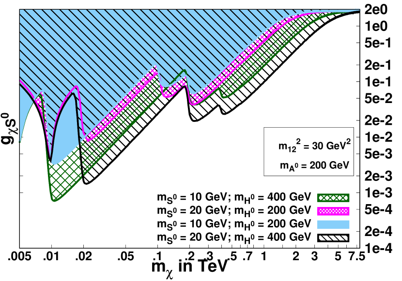
(a)

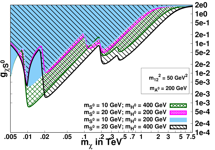
(b)

(c)

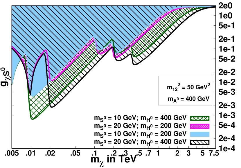
(d)

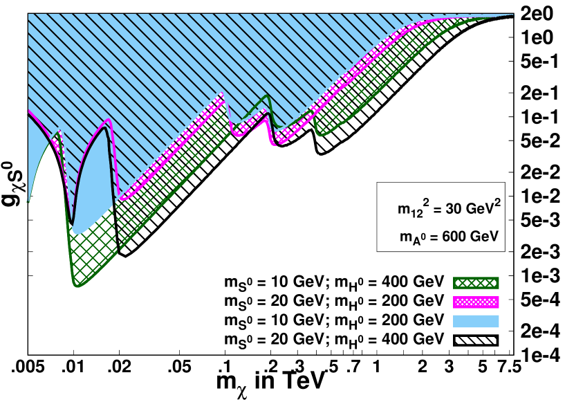
(e)

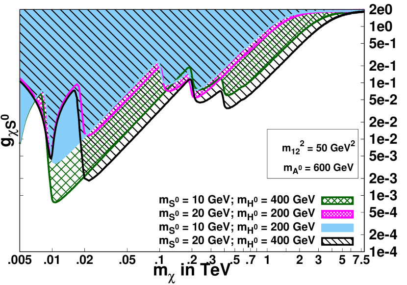
(f)

Figure 6: Figures 6(a) to 6(f) show contours on the $m_{\chi}$ - $g_{\chi S^{0}}$ plane satisfying the relic density 0.119 Ade:2015xua ; Komatsu:2014ioa for fixed $m_{H^{\pm}}$ = 600 GeV, $\delta_{13}$ = 0.2 and different choices of $m_{12}^{2}$ and $m_{A^{0}}$. All points on the contours satisfy the discrepancy $\Delta a_{\mu}=\,268(63)\,\times 10^{-11}$. In the left and right panels, we show allowed (shaded) regions for four and five combinations of $m_{S^{0}}$, $m_{H^{0}}$ respectively.

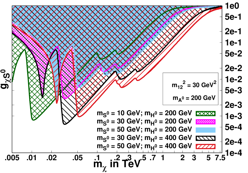
(a)

(b)

(c)

(d)

(e)

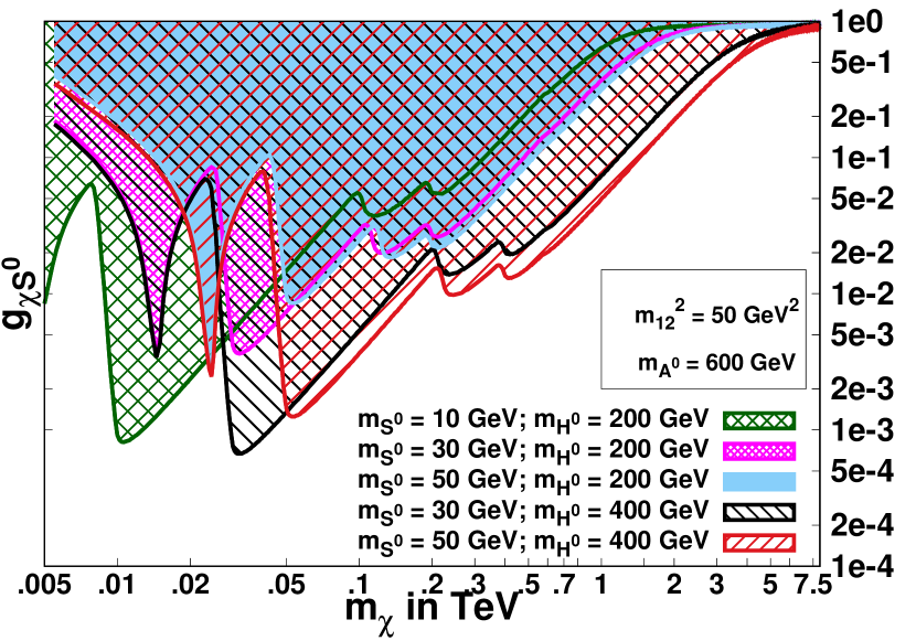
(f)

Figure 7: Figures 7(a) to 7(f) show contours on the $m_{\chi}$ - $g_{\chi S^{0}}$ plane satisfying the relic density 0.119 Ade:2015xua ; Komatsu:2014ioa for fixed $m_{H^{\pm}}$ = 600 GeV, $\delta_{13}$ = 0.4 and different choices of $m_{12}^{2}$ and $m_{A^{0}}$. All points on the contours satisfy the discrepancy $\Delta a_{\mu}=\,268(63)\,\times 10^{-11}$. In the left and right panels, we show allowed (shaded) regions for four and five combinations of $m_{S^{0}}$, $m_{H^{0}}$ respectively.

$$\frac{dn_{\chi}}{dt}+3\frac{\dot{a}}{a}\,n_{\chi}=-\langle\sigma\left|\vec{v}\right|\rangle\left(n^{2}_{\chi}-n^{2}_{\chi eq}\right)$$ (38)

where $\frac{\dot{a}}{a}=\sqrt{\frac{8\pi\rho}{3\,M_{Pl}}}$ , $\langle\sigma\left|\vec{v}\right|\rangle$ is thermally averaged cross-section and

$n^{2}_{\chi eq}={\mathbf{g}}\left(\frac{m_{\chi}T}{2\pi}\right)^{\frac{3}{2}}\exp\left[\frac{-m_{\chi}}{T}\right]$ where ${\mathbf{g}}$ is the degrees of freedom, and it is 2 for fermions. As for a massive thermal relics, freeze-out occurs when the species is non-relativistic $\left|\vec{v}\right|<<c$. Therefore, we expand $\langle\sigma\left|\vec{v}\right|\rangle$ as $\langle\sigma\left|\vec{v}\right|\rangle=a+b\left|\vec{v}\right|^{2}+\mathcal{O}(\left|\vec{v}\right|^{4})$. The Boltzmann equation can be solved to give the thermal relic density F.Tanedo

$$\Omega_{\chi}{\mathbf{h}}^{2}\simeq\frac{1.07\times 10^{9}x_{F}}{M_{Pl}\,\,\sqrt{{\mathbf{g}^{*}}(x_{F})}(a+\frac{6b}{x_{F}})}$$ (39)

where ${\mathbf{h}}$ is dimensionless Hubble parameter, ${\mathbf{g}^{*}}(x_{F})$ is total number of dynamic degrees of freedom near freeze-out temperature $T_{F}$ and $x_{F}=\frac{m_{\chi}}{T_{F}}$ is given by

$$x_{F}=\ln\left[c\,(c+2)\sqrt{\frac{45}{8}}\,\frac{{\mathbf{g}}\,M_{Pl}\,\,m_{\chi}\left(a+\frac{6\,b}{x_{F}}\right)}{2\pi^{3}\sqrt{{\mathbf{g}^{*}}\left(x_{F}\right)}\sqrt{x_{F}}}\right]$$ (40)

where $c$ is of the order 1. The thermal-averaged scattering cross-sections as a function of DM mass $m_{\chi}$ are given in the Appendix C.

To compute relic density numerically, we have used MadDM Ambrogi:2018jqj and MadGraph Alwall:2014hca . We have generated the input model file required by MadGraph using FeynRules Alloul:2013bka , which calculates all the required couplings and Feynman rules by using the full Lagrangian.

For a given charged Higgs mass of 600 GeV we depict the contours of constant relic density $\simeq$ 0.119 Ade:2015xua ; Komatsu:2014ioa in $g_{\chi S^{0}}$ (DM coupling) and $m_{\chi}$ (DM mass) plane in figure 6 corresponding to two choices of singlet scalar masses of 10 and 20 GeV for $\delta_{13}$ = 0.2 and in figure 7 corresponding to three choices of singlet scalar masses of 10, 30 and 50 GeV for $\delta_{13}$ = 0.4. The six different panels in figures 6 and 7 correspond to the following six different combinations of $\left(m_{A^{0}},m_{12}^{2}\right):$

$$\left(200\,{\rm GeV},\,30\,{\rm GeV}^{2}\right),\,\left(200\,{\rm GeV},\,50\,{\rm GeV}^{2}\right),\,\left(400\,{\rm GeV},\,30\,{\rm GeV}^{2}\right),$$

$$\left(400\,{\rm GeV},\,50\,{\rm GeV}^{2}\right),\,\left(600\,{\rm GeV},\,30\,{\rm GeV}^{2}\right)\,\,{\rm and}\,\,\left(600\,{\rm GeV},\,50\,{\rm GeV}^{2}\right).$$

The un-shaded regions in $g_{\chi S^{0}}-m_{\chi}$ plane in figures corresponding to over closing of the Universe by DM relic density contribution. The successive dips in the relic density contours arise due to opening up of additional DM annihilation channel with the increasing DM mass. Initial dip is caused by s-channel propagator. Dip observed around 0.2 TeV and 0.4 TeV are caused by opening of $\bar{\chi}\chi\rightarrow S^{0}H^{0}$ and $\bar{\chi}\chi\rightarrow H^{0}H^{0}\,(A^{0}A^{0})$ channels. The parameter sets chosen for the calculation of the relic density are consistent with the observed value of $\Delta a_{\mu}$ and measured total Higgs decay width.

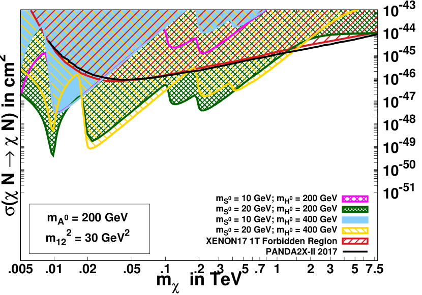
(a)

(b)

(c)

(d)

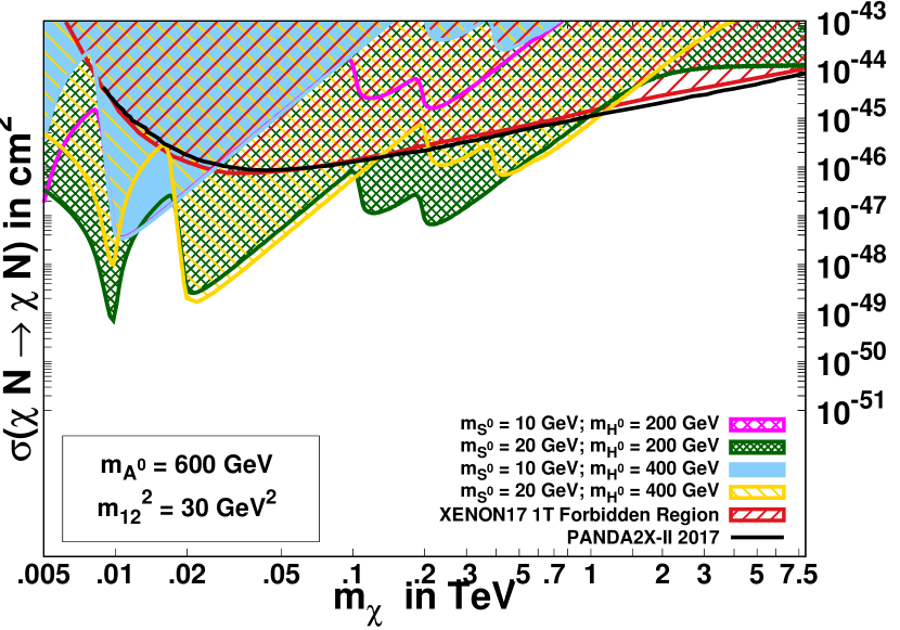
(e)

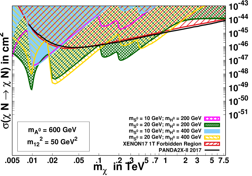
(f)

Figure 8: Figures 8(a) to 8(f) show the spin-independent DM-Nucleon cross-section variation with the $m_{\chi}$ for fixed $m_{H^{\pm}}$ = 600 GeV , $\delta_{13}$ = 0.2 and different choices of $m_{12}^{2}$ and $m_{A^{0}}$. All points on the contours satisfy the relic density 0.119 and also explain the discrepancy $\Delta a_{\mu}=\,268(63)\,\times 10^{-11}$. In the left and right panels, we plot the variation curves (bold lines) and allowed (shaded) regions for five combinations of $m_{S^{0}}$ and $m_{H^{0}}$. The upper limit from PANDA 2X-II 2017 Cui:2017nnn and XENON-1T Aprile:2015uzo ; Aprile:2017aty are also shown along with the forbidden region shaded in red.

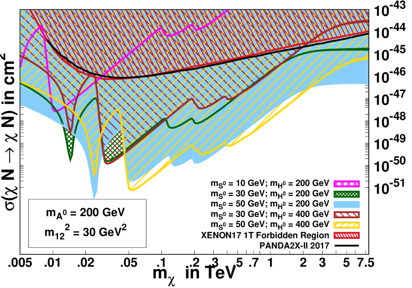
(a)

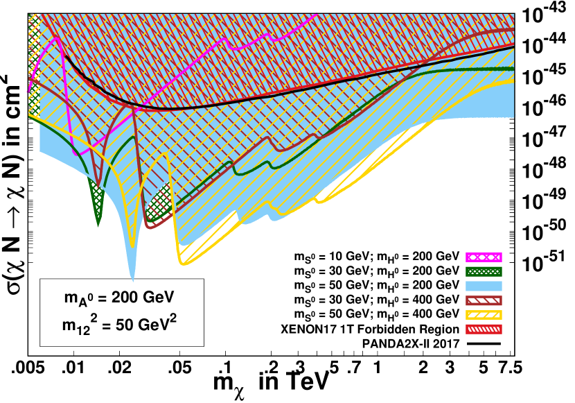
(b)

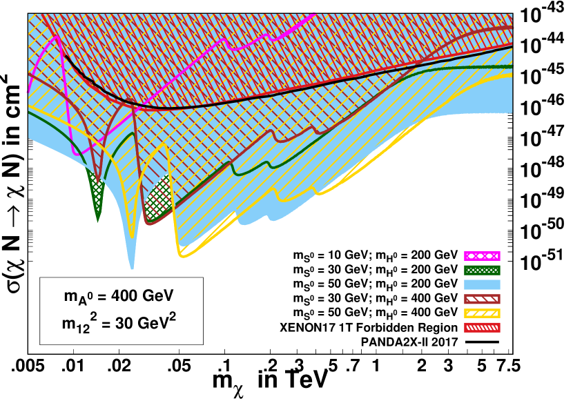
(c)

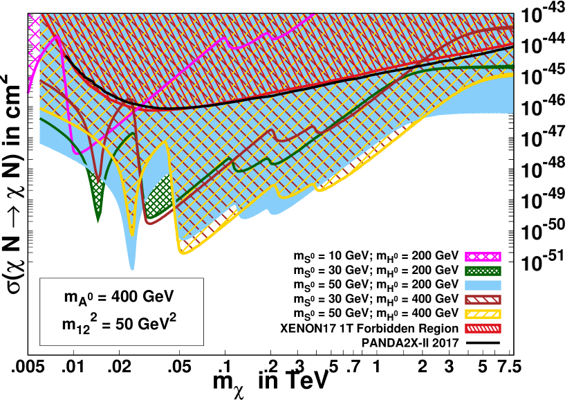
(d)

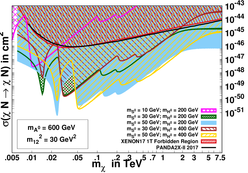
(e)

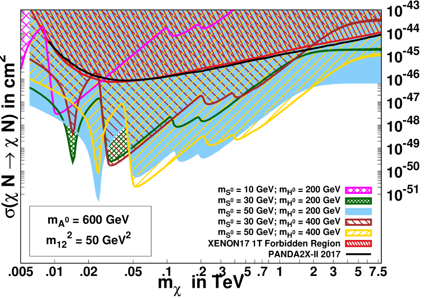
(f)

Figure 9: Figures 9(a) to 9(f) show the spin-independent DM-Nucleon cross-section variation with the $m_{\chi}$ for fixed $m_{H^{\pm}}$ = 600 GeV , $\delta_{13}$ = 0.4 and different choices of $m_{12}^{2}$ and $m_{A^{0}}$. All points on the contours satisfy the relic density 0.119 and also explain the discrepancy $\Delta a_{\mu}=\,268(63)\,\times 10^{-11}$. In the left and right panels, we plot the variation curves (bold lines) and allowed (shaded) regions for five combinations of $m_{S^{0}}$ and $m_{H^{0}}$. The upper limit from PANDA 2X-II 2017 Cui:2017nnn and XENON-1T Aprile:2015uzo ; Aprile:2017aty are also shown along with the forbidden region shaded in red.

4.2 Direct Detection

Direct detection of DM measures the recoil generated by DM interaction with matter. For the case of lepto-philic DM, we have tree level DM-Electron interaction, where DM can scatter with electron in-elastically, leading to ionization of the atom to which it is bound or elastically, where excitation of atom is succeeded by de-excitation, releasing a photon. The DM-Nucleon scattering in this model occurs at the loop level and though suppressed by one or two powers of respective coupling strengths and the loop factor, it vastly dominates over the DM-Electron and DM-Atom scattering Kopp:2009et ; Kopp:2014tsa ; DEramo:2017zqw .

The scalar spin-independent DM-Nucleon scattering are induced through the effective DM-photon, DM-quark and DM-gluon interactions which are mediated by the singlet scalar portal of the model. Following reference Kopp:2009et , we approximate the DM-Nucleon scattering cross-section through two photons by integrating out the contributions of heavier fermions running in the loop. The total cross-section Spin-Independent DM-Nucleon in this case is given as

$$\sigma^{\gamma\gamma}_{N}=\left(\frac{\alpha_{em}Z}{\pi}\right)^{2}\left[\frac{\mu^{2}_{N}}{\pi}\left(\frac{\alpha_{em}Z}{\pi m^{2}_{S^{0}}}\right)^{2}\right]\left(\frac{\pi^{2}}{12}\right)^{2}\left(\frac{\mu_{N}v}{m_{\tau}}\right)^{2}2\left(g_{\chi S^{0}}\xi^{S^{0}}_{l}\frac{m_{\tau}}{v_{0}}\right)^{2}$$ (41)

where $Z$ is the atomic number of the detector material, $\mu_{N}$ is the reduced mass of the DM-Nucleon system and $v$ is the DM velocity of the order of 10^-3.

The effective DM-gluon interactions are induced through a quark triangle loop, where, the negligible contribution of light quarks $u$, $d$ and $s$ to the loop integral can be dropped. In this approximation, the effective Lagrangian for singlet scalar-gluon interactions can be derived by integrating out contributions from heavy quarks $c$, $b$ and $t$ in the triangle loop and can be written as

$${\cal L}_{\rm eff.}^{S^{0}gg}=-\frac{\xi^{S^{0}}_{q}}{12\pi}\frac{\alpha_{s}}{v_{o}}\left\{\sum_{q=c,b,t}I_{q}\right\}G_{\mu\nu}^{a}G^{\mu\nu a}S^{0}$$ (42)

where the loop integral $I_{q}$ is given in Appendix B. The DM-gluon effective Lagrangian is the given as

$${\cal L}_{\rm eff.}^{\chi\chi gg}=\frac{\alpha_{s}(m_{S^{0}})}{12\pi}\frac{\xi^{S^{0}}_{q}g_{\chi S^{0}}}{v_{o}m^{2}_{S^{0}}}\left\{\sum_{q=c,b,t}I_{q}\right\}\bar{\chi}\chi G_{\mu\nu}^{a}G^{\mu\nu a}.$$ (43)

Using (43), the DM-gluon scattering cross-section can be computed and given as:

$$\sigma^{gg}_{N}=\left(\frac{2\xi^{S^{0}}_{q}g_{\chi S^{0}}m_{N}}{m^{2}_{S^{0}}27v_{o}}\right)^{2}\left|\sum_{q=c,b,t}I_{q}\right|^{2}\frac{2}{\pi(m_{\chi}+m_{N})^{2}}m_{N}^{2}m^{2}_{\chi}$$ (44)

To compare the cross-sections given in (41) and (44), we evaluate the ratio

$$\frac{\sigma^{\gamma\gamma}_{N}}{\sigma^{gg}_{N}}\simeq(\alpha_{em})^{4}\frac{\mu^{2}_{N}}{m^{2}_{N}}\left(\frac{\xi^{S^{0}}_{\tau}}{\xi^{S^{0}}_{q}}\right)^{2}\left(\frac{9}{8}\right)^{2}\frac{v^{2}}{c^{2}}\simeq 10^{-6}-10^{-10}.$$ (45)

Thus even though the effective DM-quark coupling is suppressed by $\tan^{2}\beta$ w.r.t that of DM-lepton coupling, the scattering cross-sections induced via the singlet coupled to the quark-loop dominates over the $\sigma^{\gamma\gamma}_{N}$ due to suppression resulting from the fourth power of the electromagnetic coupling.

We convolute the DM-quark and DM-gluon scattering cross-sections with the quark form factor $F^{q_{i}/N}(q^{2})$ and gluon form factor $F^{g/N}(q^{2})$ respectively to compute nuclear recoil energy observed in the experiment. However, this form factor is extracted at low $q^{2}\ll m^{2}_{N}$ Bishara:2017nnn ; DelNobile:2013sia ; Dutta:2017jfj . The form factors are defined as

$$\left\langle N^{\prime}\left|\frac{\alpha_{s}}{12\pi}{G^{a}}^{\mu\nu}G^{a}_{\mu\nu}\right|N\right\rangle = F^{g/N}(q^{2})\bar{u}^{\prime}_{N}u_{N}$$ (46a)

$$\left\langle N^{\prime}\left|m_{q_{i}}\bar{q_{i}}q_{i}\right|N\right\rangle = F^{q_{i}/N}(q^{2})\bar{u}^{\prime}_{N}u_{N}$$ (46b)

Since, $m_{N}\equiv\sum_{u,d,s}\left\langle N\left|m_{q}\bar{q}q\right|N\right\rangle-\frac{9\alpha_{S}}{8\pi}\left\langle N\left|{G^{a}}^{\mu\nu}{G^{a}}_{\mu\nu}\right|N\right\rangle$, the gluon form factor can be expressed as

$$F^{g/N}=1-\sum_{u,d,s}\frac{F^{q_{i}/N}_{S}(q^{2})}{m_{N}}=-\frac{1}{m_{N}}\frac{9\alpha_{s}}{8\pi}\left\langle N\left|{G^{a}}^{\mu\nu}{G^{a}}_{\mu\nu}\right|N\right\rangle$$ (47)

The $F^{g/N}$ is found to be $\approx$ 0.92 using the values for $F^{q_{i}/N}_{S}(q^{2})$ as quoted in the literature DelNobile:2013sia . Thus, at the low momentum transfer the quartic DM-gluon $\left(\chi\chi gg\right)$ effective interaction induced through relatively heavy quarks dominates over the quartic DM-quark $\left(\chi\chi qq\right)$ effective interactions for light quarks in the direct-detection experiments.

Using the expression 44 we have plotted the spin-independent DM-Nucleon scattering cross-section as a function of the DM mass $m_{\chi}$. Figures 8 and 9 corresponding to mixing angle $\delta_{13}$=0.2 and $\delta_{13}$=0.4 respectively. The parameter sets used in the computation of direct detection cross-section are consistent with the observed relic density as given in figures 6 and 7. Different panels in figures 8 and 9 show combinations of $m_{A^{0}}$ and $m^{2}_{12}$. In each panel different combinations of $m_{S^{0}}$ and $m_{H^{0}}$ are used as shown. Current bounds on spin-independent interactions from experiments like PANDA 2X-II 2017 Cui:2017nnn and XENON-1T Aprile:2015uzo ; Aprile:2017aty are also shown. It can be seen that most of the parameter space for $m_{S^{0}}$ less than 10 GeV is ruled out by the current bounds.

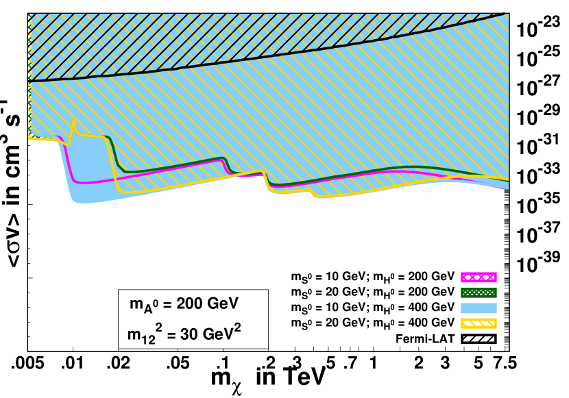
(a)

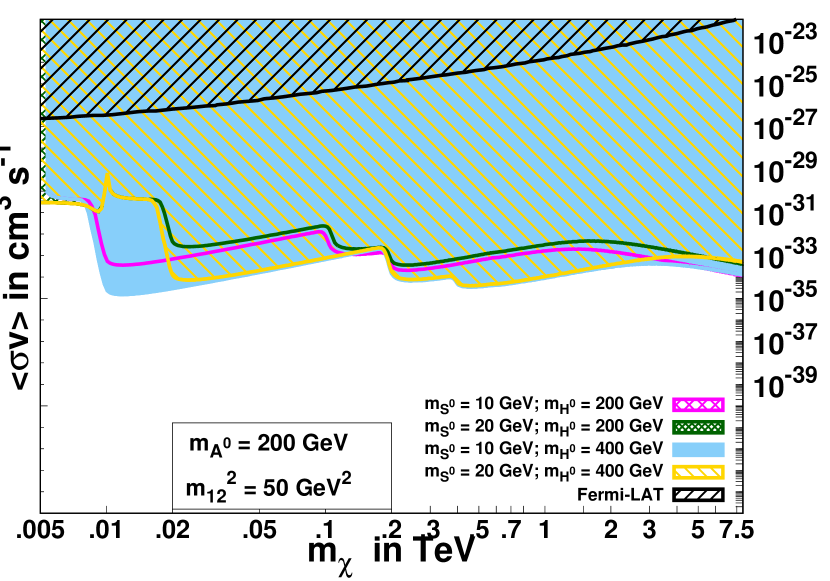
(b)

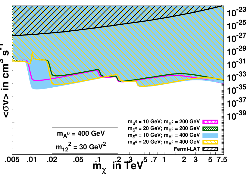
(c)

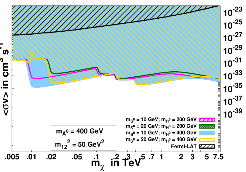
(d)

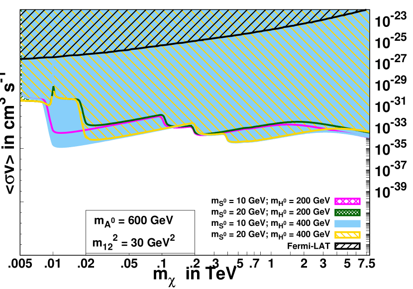
(e)

(f)

Figure 10: Figures 10(a) to 10(f) show the velocity-averaged scattering cross-section $<\sigma v>_{\tau^{+}\tau^{-}}$ variation with the $m_{\chi}$ for fixed $m_{H^{\pm}}$ = 600 GeV, $\delta_{13}$ = 0.2 and different choices of $m_{12}^{2}$ and $m_{A^{0}}$. All points on the contours satisfy the relic density 0.119 and also explain the discrepancy $\Delta a_{\mu}=\,268(63)\,\times 10^{-11}$. In the left and right panels, we plot the variation curves (bold lines) and allowed (shaded) regions for four five combinations of $m_{S^{0}}$ and $m_{H^{0}}$. The upper limit on velocity-averaged annihilation cross-section observed from Fermi-LAT Ackermann:2015zua is shown.

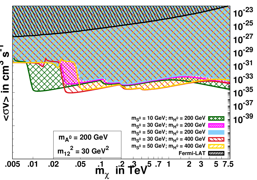
(a)

(b)

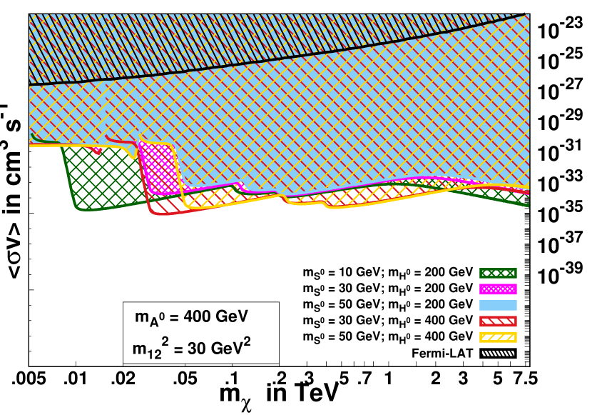
(c)

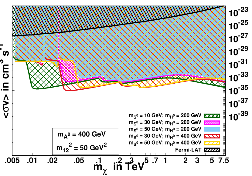
(d)

(e)

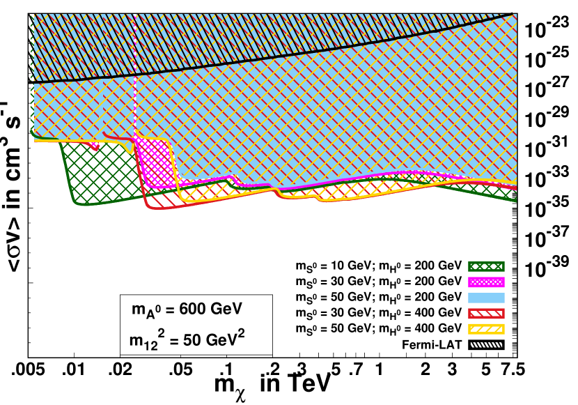
(f)

Figure 11: Figures 11(a) to 11(f) show the velocity-averaged scattering cross-section $<\sigma v>_{\tau^{+}\tau^{-}}$ variation with the $m_{\chi}$ for fixed $m_{H^{\pm}}$ = 600 GeV, $\delta_{13}$ = 0.4 and different choices of $m_{12}^{2}$ and $m_{A^{0}}$. All points on the contours satisfy the relic density 0.119 and also explain the discrepancy $\Delta a_{\mu}=\,268(63)\,\times 10^{-11}$. In the left and right panels, we plot the variation curves (bold lines) and allowed (shaded) regions for four five combinations of $m_{S^{0}}$ and $m_{H^{0}}$. The upper limit on velocity-averaged annihilation cross-section observed from Fermi-LAT Ackermann:2015zua is shown.

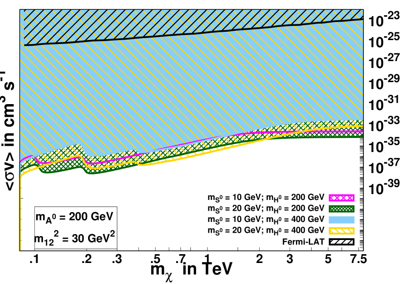
(a)

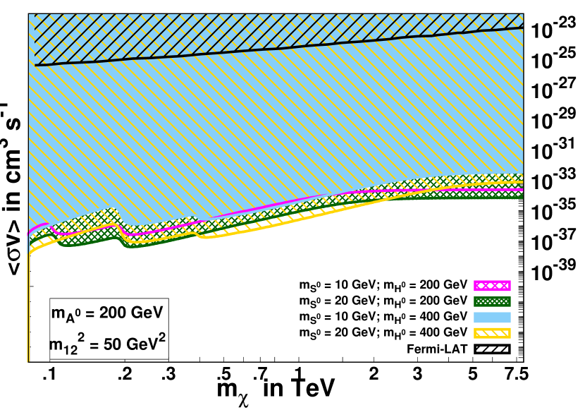
(b)

(c)

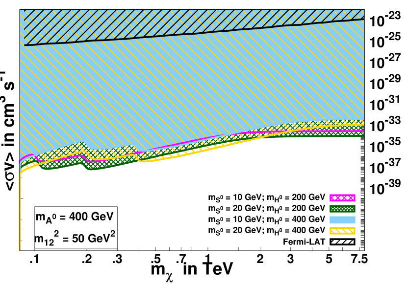
(d)

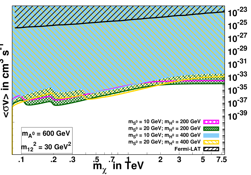
(e)

(f)

Figure 12: Figures 12(a) to 12(f) show the velocity-averaged scattering cross-section $<\sigma v>_{W^{+}W^{-}}$ variation with the $m_{\chi}$ for fixed $m_{H^{\pm}}$ = 600 GeV, $\delta_{13}$ = 0.2 and different choices of $m_{12}^{2}$ and $m_{A^{0}}$. All points on the contours satisfy the relic density 0.119 and also explain the discrepancy $\Delta a_{\mu}=\,268(63)\,\times 10^{-11}$. In the left and right panels, we plot the variation curves (bold lines) and allowed (shaded) regions for five combinations of $m_{S^{0}}$ and $m_{H^{0}}$ . The upper limit on velocity-averaged annihilation cross-section observed from Fermi-LAT Ackermann:2015zua is shown.

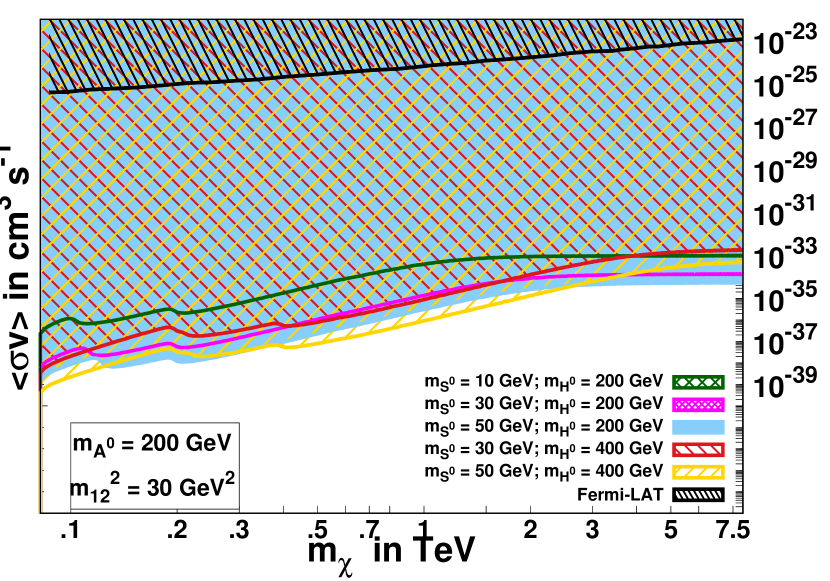
(a)

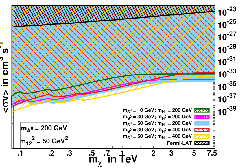
(b)

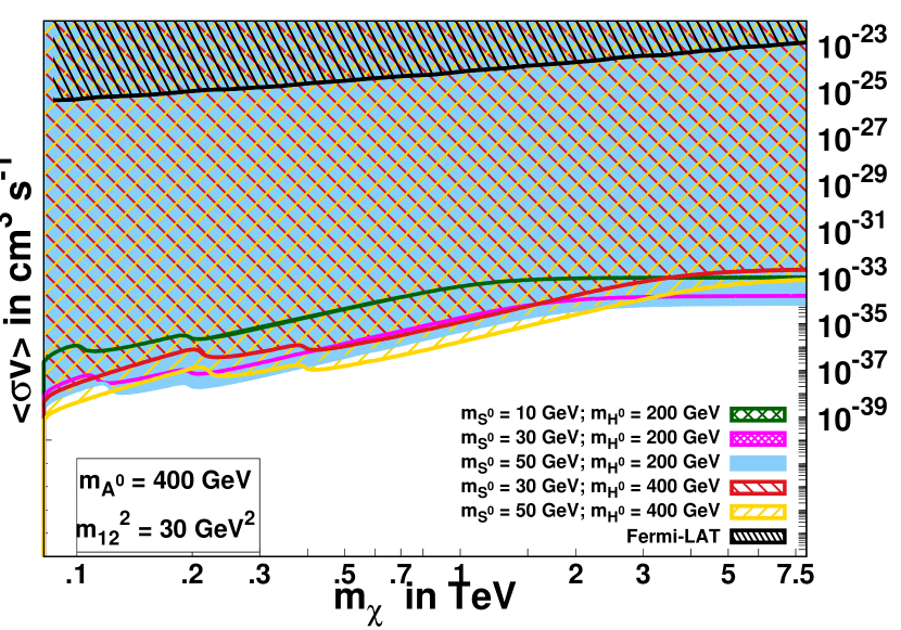
(c)

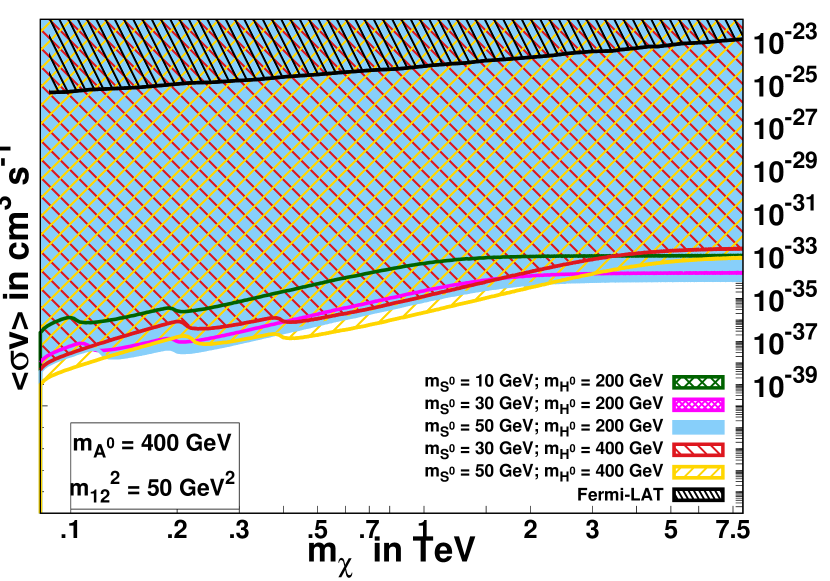
(d)

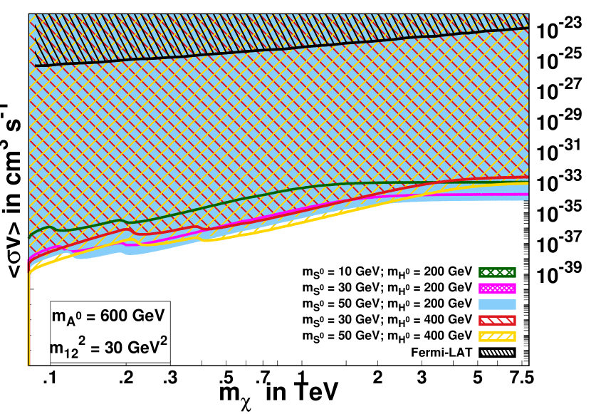
(e)

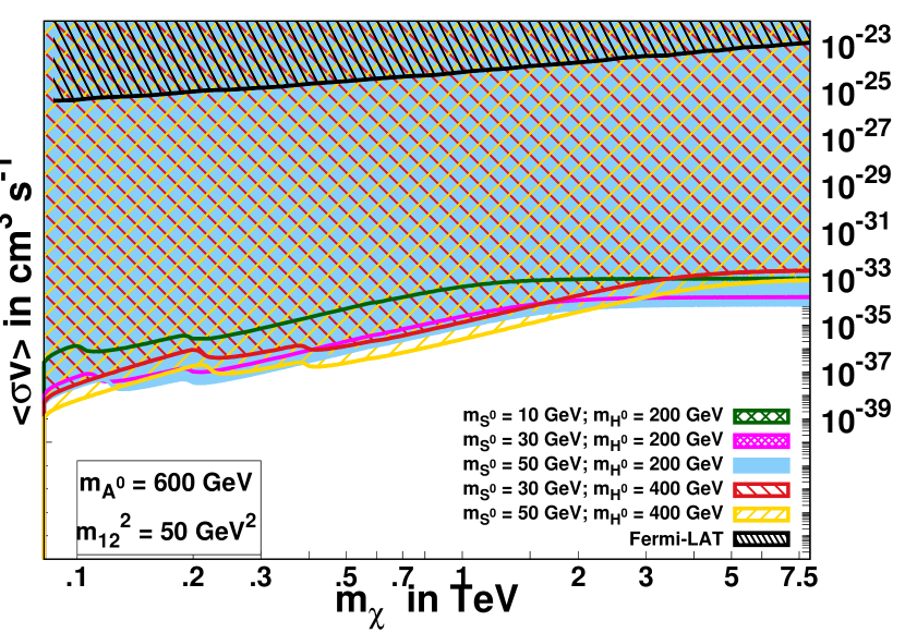
(f)

Figure 13: Figures 13(a) to 13(f) show the velocity-averaged scattering cross-section $<\sigma v>_{W^{+}W^{-}}$ variation with the $m_{\chi}$ for fixed $m_{H^{\pm}}$ = 600 GeV, $\delta_{13}$ = 0.4 and different choices of $m_{12}^{2}$ and $m_{A^{0}}$. All points on the contours satisfy the relic density 0.119 and also explain the discrepancy $\Delta a_{\mu}=\,268(63)\,\times 10^{-11}$. In the left and right panels, we plot the variation curves (bold lines) and allowed (shaded) regions for five combinations of $m_{S^{0}}$ and $m_{H^{0}}$ . The upper limit on velocity-averaged annihilation cross-section observed from Fermi-LAT Ackermann:2015zua is shown.

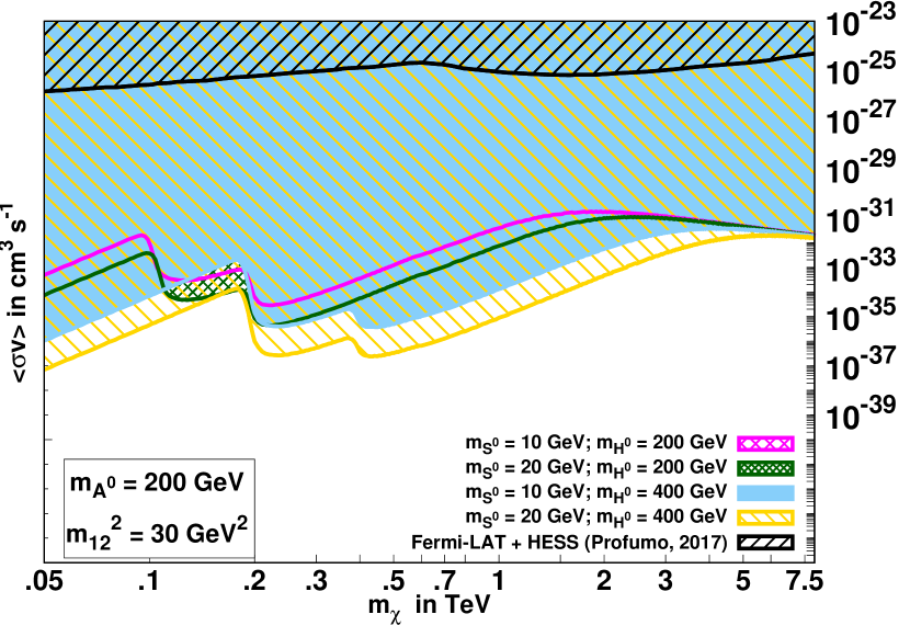
(a)

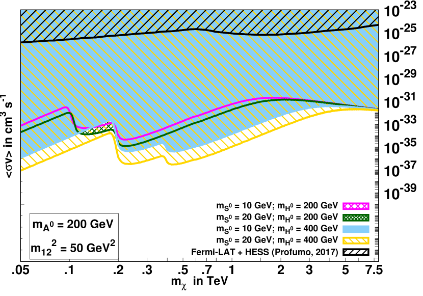
(b)

(c)

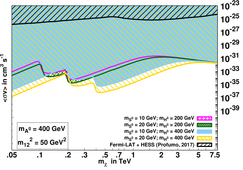
(d)

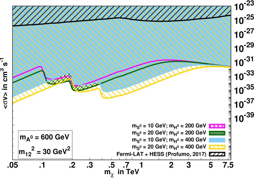
(e)

(f)

Figure 14: Figures 14(a) to 14(f) show the velocity-averaged scattering cross-section $<\sigma v>_{S^{0}S^{0}}$ variation with the $m_{\chi}$ for fixed $m_{H^{\pm}}$ = 600 GeV, $\delta_{13}$ = 0.2 and and different choices of $m_{12}^{2}$ and $m_{A^{0}}$. All points on the contours satisfy the relic density 0.119 and also explain the discrepancy $\Delta a_{\mu}=\,268(63)\,\times 10^{-11}$. In the left and right panels, we plot the variation curves (bold lines) and allowed (shaded) regions for five combinations of $m_{S^{0}}$ and $m_{H^{0}}$. The upper limit on velocity-averaged annihilation cross-section for the process $\chi\chi\rightarrow S^{0}S^{0}$ computed from 4$\tau$ final states from Fermi-LAT dataProfumo:2017obk is shown.

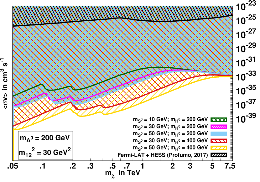
(a)

(b)

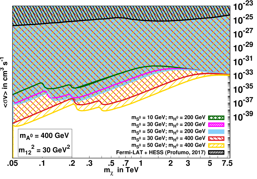
(c)

(d)

(e)

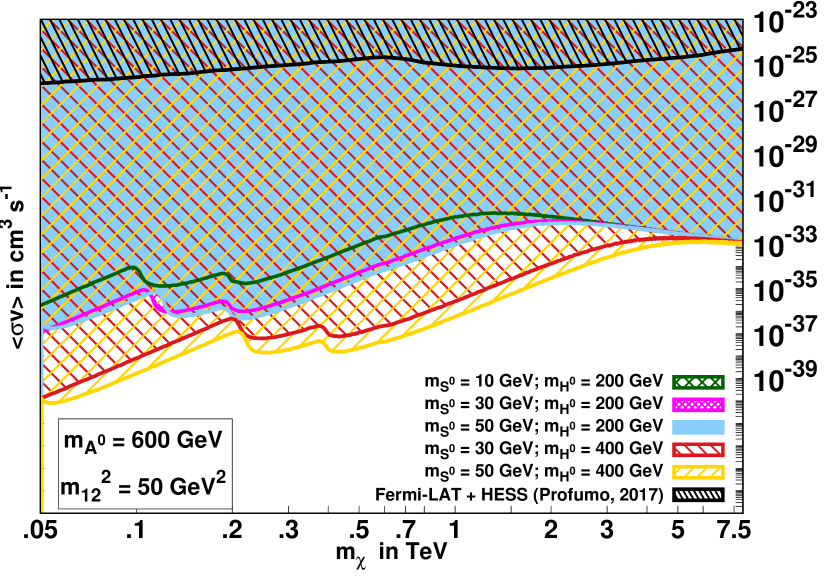
(f)

Figure 15: Figures 15(a) to 15(f) show the velocity-averaged scattering cross-section $<\sigma v>_{S^{0}S^{0}}$ variation with the $m_{\chi}$ for fixed $m_{H^{\pm}}$ = 600 GeV, $\delta_{13}$ = 0.4 and and different choices of $m_{12}^{2}$ and $m_{A^{0}}$. All points on the contours satisfy the relic density 0.119 and also explain the discrepancy $\Delta a_{\mu}=\,268(63)\,\times 10^{-11}$. In the left and right panels, we plot the variation curves (bold lines) and allowed (shaded) regions for five combinations of $m_{S^{0}}$ and $m_{H^{0}}$. The upper limit on velocity-averaged annihilation cross-section for the process $\chi\chi\rightarrow S^{0}S^{0}$ computed from 4$\tau$ final states from Fermi-LAT data Profumo:2017obk is shown.

4.3 Indirect detection

Observations of diffused gamma rays from the regions of our Galaxy, such as Galactic Center (GC) and dwarf spheroidal galaxies (dsphs), where DM density appears to be high, impose bounds on DM annihilation to SM particles. Experiments like Fermi-LAT TheFermi-LAT:2015kwa ; Ackermann:2015zua and H.E.S.S. Moulin:2007qw have investigated DM annihilation as a possible source of the incoming photon-flux. These experiments provide us with an upper-limit to velocity-averaged scattering cross-section for various channels, which can attribute to the observed photon-flux.

DM annihilations contribute to the photon-flux through Final State Radiation (FSR) and radiative decays Mazziotta:2014ada ; Ackermann:2013yva from leptonic channels in lepto-philic models. FSR contributions are important in understanding the photon-spectra from DM annihilations to charged final states and therefore are instrumental in calculation of the observed bounds by experiments like Fermi-LAT Ackermann:2015zua ; Ackermann:2013yva ; Essig:2009jx ; Bringmann:2007nk . The radiation emitted by the charged relativistic final state fermions $f$ in the annihilation process $\bar{\chi}+\chi\rightarrow f+\bar{f}+\gamma$ are approximately collinear with the charged fermions. In this regime, the differential cross-section for the real emission process can be factorized into the a collinear factor and cross-section $\sigma(\chi\chi\to f\bar{f})$ as discussed in the reference Birkedal:2005ep .

$$\begin{array}[]{rcl}\frac{d\sigma(\chi\chi\,\to\,f\bar{f}\gamma)}{dx}\approx\frac{\alpha_{em}Q_{f}^{2}}{\pi}\,{\cal F}_{f}(x)\,\log\left(\frac{s(1-x)}{m_{f}^{2}}\right)\sigma(\chi\chi\to f\bar{f}),\end{array}$$ (48)

where $Q_{f}$ and $m_{f}$ are the electric charge and the mass of the $f$ particle, $s$ is the center-of-mass energy, and $x=2E_{\gamma}/\sqrt{s}$. For fermion final states, the splitting function ${\cal F}$ is given by

$$\begin{array}[]{rcl}{\cal F}_{f}(x)=\frac{1+\left(1-x\right)^{2}}{x}\end{array}$$ (49)

The suppression factor of $p$-wave suppressed thermal averaged cross-section $\left\langle\sigma(\chi\chi\to f\bar{f})\,v\right\rangle$ is mitigated in the thermal averaged cross-section of the real emission process $\left\langle\sigma(\chi\chi\to f\bar{f}\gamma)\,v\right\rangle$ by the virtue of collinear factor given in equation (48).

In the present model, the fermionic DM can annihilate to SM particles via $s-channnel$ through the scalar portal as well as to a pair of singlet scalars through $t-channel$ diagrams. Recently authors of the reference Siqueira:2019wdg ; Queiroz:2019acr explored the discovery potential of the pair production of such lepto-philic scalars which pre-dominantly decay into pairs of charged leptons at Cherenkov Telescope Array (CTA). Given the spectrum of pair produced SM particles through single scalar mediator and into two pairs of charged leptons through scalar pair production, we should be able to simulate the expected DM fluxes which will enable us to get the upper limits on the annihilation cross section for a given mediator mass in the model.

We calculate the velocity averaged cross-sections analytically for the annihilation processes $\chi\,\bar{\chi}\to f\bar{f}$, $\chi\,\bar{\chi}\to Z^{0}Z^{0}$, $\chi\,\bar{\chi}\to W^{+}W^{-}$, $\chi\,\bar{\chi}\to\gamma\gamma$ and $\chi\,\bar{\chi}\to H_{i}\,H_{j}$ and are given in equations (LABEL:thermalfermion), (66), (67), (69) and (70) respectively where $H_{i}\equiv h^{0},\,H^{0},\,S^{0}$ and $A^{0}$ are the scalars of the model. In addition, the velocity averaged annihilation cross-section for $\chi\,\bar{\chi}\to S^{0}S^{0}$ through the $t$ and $u$ channel diagrams are given in (71). We observe that the velocity averaged scattering cross-sections for all these processes are $p$-wave suppressed and are, therefore, sensitive to the choice of velocity distribution of the DM in the galaxy.

The annihilation channels to fermions are proportional to the Yukawa coupling of the fermions with $S^{0}$. We present the analysis for the most dominant $s-channel$ annihilation process $\chi\,\bar{\chi}\to\tau^{+}\tau^{-}$, which is enhanced due to its coupling strength being proportional to $m_{\tau}\tan\beta$ and plot the variation of the velocity averaged scattering cross-section $\left\langle\sigma v\right\rangle(\chi\bar{\chi}\rightarrow\tau^{+}\tau^{-})$ as a function of the DM mass in figures 10 and 11 for mixing angle $\delta_{13}$ = 0.2 and 0.4 respectively. The coupling $g_{\chi S^{0}}$ for a given DM mass and all other parameters are chosen to satisfy the observed relic density and electro-weak constraints as shown in the figures 6 and 7. Annihilation of DM pairs to gauge Bosons are proportional to the square of their masses and therefore it is the second dominant process followed by the annihilation to $\tau\pm$ pairs. Similarly, we show the variation of the velocity averaged scattering cross-section $\left\langle\sigma v\right\rangle(\chi\bar{\chi}\rightarrow W^{+}W^{-})$ as a function of the DM mass in figures 12 and 13 for $\delta_{13}$ = 0.2 and 0.4 respectively. The DM pair annihilation to photons is loop suppressed and is not discussed further. The $s$ channel mediated DM pair annihilation to pair of scalars in the theory involve the triple scalar couplings, which are experimentally constrained and are therefore suppressed.

As mentioned above, the t-channel pair production of singlet scalars dominates over the other channels. The $S^{0}$ pair production through its decay to dominant $\tau$ pairs will modify the $\gamma$ ray spectrum that one would have expected from the two body decay processes. We plot the velocity averaged scattering cross-section $\left\langle\sigma v\right\rangle(\chi\bar{\chi}\rightarrow S^{0}S^{0})$ as a function of the DM mass which satisfies the relic density constraint in figures 14 and 15 for $\delta_{13}$ = 0.2 and 0.4 respectively with all the other parameters fixed from the observed relic density and electro-weak constraints. The experimental upper limit on velocity-averaged annihilation cross-section for the process $\chi\chi\rightarrow S^{0}S^{0}$ for the varying DM mass are derived from the upper limits on the events contributed to 4$\tau$ final states at Fermi-LAT Profumo:2017obk and shown in figures 14 and 15.

We find that the annihilation cross-sections for all these processes are three or more orders of magnitude smaller than the current upper-bounds from Fermi-Lat data Ackermann:2015zua ; Profumo:2017obk .

5 Summary

In this article we have made an attempt to address the observed discrepancy in anomalous magnetic moment of muon by considering a lepto-philic type X 2-HDM and a singlet scalar portal for fermionic DM. We have presented the model in such a manner where most of it’s scalar sector parameters can be constrained in terms of the lower bound on the physical neutral and charged scalar’s masses derived from the direct and indirect searches at LEP and LHC.

The model is analysed in the alignment limit, where one of its scalar is identified with the Higgs Boson of SM and the Yukawa couplings of fermions with the singlet scalar are found to be proportional to mass of the fermions i.e. non-universal. It is then validated with low energy constraints. We have illustrated the constraints from anomalous magnetic moment in figures 1 and 2 and fixed the parameters $\tan\beta$ and $\delta_{23}$ for a given $\delta_{13}$. We have considered two choices 0.2 and 0.4 respectively for the mixing angle $\delta_{13}$. Contrary to the results obtained in reference Agrawal:2014ufa for the singlet scalar with mass lying between 10 - 300 MeV with universal couplings to leptons, this study establishes the acceptability of the model to explain the discrepancy $\Delta a_{\mu}$ for singlet scalar mass lying between 10 GeV $\leq$ $m_{S^{0}}$ $\leq$ 80 GeV with couplings to leptons being non-universal. The requirement of the Yukawa coupling $H^{0}\,\tau^{+}\tau^{-}$ to remain perturbative further imposes an upper limit $\tan\beta\leq 485$ which in turn provides the upper bound on the allowed mass range of singlet scalars to be $\sim 80$ GeV.

Exclusion limits on the couplings of SM gauge Bosons with the singlet scalars are obtained from the process $e^{+}e^{-}\to Z^{0}S^{0}$ at LEP-II experiment and have been displayed in table 2 for some chosen singlet scalar masses.

Validation of the model is further subjected to the observed total Higgs decay width at LHC pdg2018Higgs ; Khachatryan:2016ctc . It is shown that the parameter $m_{12}^{2}$, which has no bearing on the $\Delta a_{\mu}$, can now be constrained from the from upper bound on the triple scalar coupling involved in the decay of SM like Higgs to a pair of singlet scalars $h^{0}\to S^{0}S^{0}$. The observed total decay width of SM like Higgs $h^{0}$ restricts this additional channel and put a upper limit on the partial decay width, which has been shown in figures 3 for $\delta_{13}$ = 0.2 and in figures 4 and 5 $\delta_{13}$ = 0.4 respectively. We have found that in the probed region of interest for singlet scalar mass, $m_{12}^{2}$ greater than 100 GeV² and less than 0 GeV² are forbidden.

We have addressed reasons for which there can be a deviation from SM predicted universality in lepton-gauge Boson couplings. The precision constraints are also discussed for our model and found that corrections are suppressed due to the smallness of mixing angle.

We augment our analysis by including a fermionic DM candidate $\chi$ and compute the relic density which are depicted in figures 6 & 7 for $\delta_{13}$ = 0.2 and 0.4 respectively. The parameter sets chosen corresponding to points lying on contours satisfying relic density of 0.119 also fulfill the $\Delta a_{\mu}$ discrepancy and are consistent with the total Higgs decay width observed at LHC and LEP data.

The scalar portal induced DM interactions are now probed in the Direct-detection experiment by the DM-nucleon scattering propelled through the gluons. The variation of spin-independent scattering cross-sections with the DM mass are shown in figures 8 and 9 for $\delta_{13}$ = 0.2 and 0.4 respectively. It can be seen that most of the parameter space for $m_{S^{0}}$ lighter than 10 GeV is excluded by current Direct-detection constraints from PANDA 2X-II and XENON-1T experiments.

The velocity averaged cross-sections for dominant DM pair annihilation channels like $\tau^{+}\tau^{-}$, $W^{+}W^{-}$, $S^{0}S^{0}$ and $\gamma\gamma$ are analytically derived, analysed and compared with the available space borne indirect-detection experiments. The velocity averaged cross-sections variation w.r.t DM mass are shown for $\delta_{13}$ = 0.2 and 0.4 in figures 10 and 11 respectively for $\chi\bar{\chi}\to\tau^{+}\tau^{-}$, in figures 12 and 13 respectively for $\chi\bar{\chi}\to W^{+}W^{-}$, in figures 14 and 15 respectively for $\chi\bar{\chi}\to S^{0}S^{0}$. We find that the contribution to the gamma ray spectrum from the most dominant annihilation channel to $\tau^{\pm}$ pairs is at least three orders of magnitude lower than the current reach for the DM mass varying between 5 GeV - 8 TeV.

In conclusion the lepton-specific type X 2-HDM model with a singlet scalar portal for fermionic dark matter is capable of explaining both the observed discrepancy in the anomalous magnetic moment of the muon and the observed relic density. This model with the shrunk parameter space after being constrained by low energy experiments, LEP Data, observed total decay width of Higgs at LHC and constrained by dark matter detection experiments can now be tested at the ongoing and upcoming collider searches.

Appendix A Model Parameters

The parameters used in the Lagrangian for lepto-philic 2-HDM and dark matter portal singlet scalar given in equation 3 are expressed in terms of the physical scalar masses, mixing angles $\alpha$ and $\beta$ and the model parameter $m_{12}^{2}$.

$$m^{2}_{11} = -\frac{1}{2}\left[m_{H^{0}}^{2}\cos^{2}\alpha+m_{h^{0}}^{2}\sin^{2}\alpha+\left\{\sin\alpha\cos\alpha\left(m_{H^{0}}^{2}-m_{h^{0}}^{2}\right)-2\,m^{2}_{12}\right\}\tan\beta\right]$$ (50)

$$m^{2}_{22} = -\frac{1}{2}\left[m_{h^{0}}^{2}\cos^{2}\alpha+m_{H^{0}}^{2}\sin^{2}\alpha+\left\{\sin\alpha\cos\alpha\left(m_{H^{0}}^{2}-m_{h^{0}}^{2}\right)-2\,m^{2}_{12}\right\}\cot\beta\right]$$ (51)

$$\lambda_{1} = \frac{1}{v_{o}^{2}\cos^{2}\beta}\left[m_{H^{0}}^{2}\cos^{2}\alpha+m_{h^{0}}^{2}\sin^{2}\alpha-m^{2}_{12}\tan\beta\right]$$ (52)

$$\lambda_{2} = \frac{1}{v_{o}^{2}\sin^{2}\beta}\left[m_{h^{0}}^{2}\cos^{2}\alpha+m_{H^{0}}^{2}\sin^{2}\alpha-m^{2}_{12}\cot\beta\right]$$ (53)

$$\lambda_{3} = \frac{2}{v_{o}^{2}\,\sin\left(2\,\beta\right)}\left[\sin\alpha\cos\alpha\left(m_{H^{0}}^{2}-m_{h^{0}}^{2}\right)-m^{2}_{12}+\,m_{H^{+}}^{2}\sin\left(2\,\beta\right)\right]$$ (54)

$$\lambda_{4} = \frac{1}{v_{o}^{2}\sin\left(2\,\beta\right)}\left[2m^{2}_{12}+\left(m_{A^{0}}^{2}-2\,m_{H^{+}}^{2}\right)\sin\left(2\,\beta\right)\right]$$ (55)

$$\lambda_{5} = \frac{1}{v_{o}^{2}\sin\left(2\,\beta\right)}\left[2\,m^{2}_{12}-m_{A^{0}}^{2}\,\sin\left(2\,\beta\right)\right]$$ (56)

Appendix B Decay widths of the singlet scalar $S^{0}$

The tree level partial decay widths of the scalar mediator are computed and are given by:

$$\Gamma(S^{0}\rightarrow f\,\bar{f})=\frac{N_{c}}{8\,\pi}\left(\frac{\xi^{S}_{f}m_{f}}{v_{o}}\right)^{2}\,\,\,m_{S^{0}}\,\,\,\left(1-\frac{4m_{f}^{2}}{m_{S^{0}}^{2}}\right)^{3/2}\,\,\,\theta\left(m_{S^{0}}-2\,mf\right)$$ (57)

where $N_{c}$ = 1 for leptons and 3 for quarks

$$\Gamma(S^{0}\rightarrow W^{+}\,W^{-}) = \frac{(\xi^{S^{0}}_{V})^{2}}{16\,\pi\,v_{o}^{2}}\,m_{S^{0}}^{3}\,\left(1-\frac{4m_{W}^{2}}{m_{S^{0}}^{2}}\right)^{1/2}\,\left[12\,\left(\frac{m_{W}}{m_{S^{0}}}\right)^{4}-4\,\left(\frac{m_{W}}{m_{S^{0}}}\right)^{2}+1\right]$$ (58)

$$\times\theta\left(m_{S^{0}}-2\,m_{W}\right)$$

$$\Gamma(S^{0}\rightarrow Z^{0}\,Z^{0}) = \frac{1}{2}\,\,\Gamma(S^{0}\rightarrow W^{+}W^{-})\,\,\,{\rm with}\,\,m_{W}\rightarrow m_{Z}$$ (59)

$$\Gamma(S^{0}\rightarrow\chi\,\bar{\chi}) = \frac{g_{\chi S^{0}}^{2}}{8\pi}\,\,\,m_{S^{0}}\,\,\,\left(1-\frac{4m_{\chi}^{2}}{m_{S^{0}}^{2}}\right)^{3/2}\,\,\,\theta\left(m_{S^{0}}-2\,m_{\chi}\right)$$ (60)

The one loop induced partial decay width of the scalar to gluons in this model arises mainly from relatively heavy quarks and is given by

$$\Gamma(S^{0}\rightarrow gg)=\left(\frac{m_{t}\xi^{S^{0}}_{q}}{v_{o}}\right)^{2}\,\,\frac{\alpha_{s}^{2}}{72\,\pi^{3}}\,\,\,\frac{m_{S^{0}}^{3}}{m_{t}^{2}}\,\,\,\,\left|\sum_{q=c,b,t}I_{q}\right|^{2}$$ (61)

For the case of photons it is given by

$$\Gamma(S^{0}\rightarrow\gamma\gamma)=\frac{m_{S^{0}}^{3}}{16\pi v^{2}_{0}}\,\,\left(\frac{\alpha_{em}}{\pi}\right)^{2}\left|\sum_{q}\xi^{S^{0}}_{q}Q^{2}_{q}I_{q}+\sum_{l}\xi^{S^{0}}_{l}Q^{2}_{q}I_{q}-\xi^{S^{0}}_{W^{\pm}}I_{W^{\pm}}+C_{SH^{+}H^{-}}\frac{v_{o}}{2m^{2}_{H^{\pm}}}I_{H^{\pm}}\right|^{2}$$ (62)

The integrals are given as

$$I_{q}=3[2\lambda_{q}+\lambda_{q}(4\lambda_{q}-1)f(\lambda_{q})]; I_{l}=2\lambda_{q}+\lambda_{q}(4\lambda_{q}-1)f(\lambda_{q});$$

$$I_{W}=3\lambda_{W}(1-2\lambda_{W})f(\lambda_{W})-\lambda_{W}-\frac{1}{2}; I_{H^{\pm}}=-\lambda_{H^{\pm}}[1+2\lambda_{H^{\pm}}f({H^{\pm}})].$$ (63)

The integrals are defined in terms of dimensionless parameter $\lambda_{i}=m^{2}_{i}/m^{2}_{S^{0}}$ and its function $f(\lambda)$ as

$$f(\lambda) = -2\left(sin^{-1}\frac{1}{2\sqrt{\lambda}}\right)^{2},for\,\lambda>\frac{1}{4}$$ (64)

$$= \frac{1}{2}\left(\ln\frac{\eta^{+}}{\eta^{-}}\right)^{2}-\frac{\pi^{2}}{2}-i\pi\frac{\eta^{+}}{\eta^{-}},\,for\,\lambda<\frac{1}{4}$$

with $\eta^{\pm}=\frac{1}{2}\pm\sqrt{\frac{1}{4}-\lambda}$.

Appendix C Thermally averaged scattering cross-sections

We compute the thermal averaged annihilation cross-section of the fermionic DM via the singlet scalar portal $S^{0}$ to the SM final states. These processes contributes to the relic density of the universe and are directly used in computing the annihilation cross-section for indirect detection of the DM.

$$\left\langle\sigma(\chi\bar{\chi}\rightarrow f\bar{f})\,v\right\rangle = \left(\frac{m_{f}\xi^{S^{0}}_{f}}{v_{o}}\right)^{2}g_{\chi S^{0}}^{2}\,\frac{1}{4\pi}\,\left(1-\frac{m_{l}^{2}}{m_{\chi}^{2}}\right)^{\frac{3}{2}}\frac{m_{\chi}^{2}}{(4m_{\chi}^{2}-m_{\phi}^{2})^{2}}\left(\frac{3}{x_{f}}\right)\theta\left(m_{\chi}-m_{f}\right)$$

$$\left\langle\sigma\left(\chi\bar{\chi}\rightarrow Z^{0}Z^{0}\right)\,v\right\rangle = \left(\frac{\xi_{V}^{S^{0}}}{v_{o}}\right)^{2}\frac{g_{\chi S^{0}}^{2}}{8\pi}\sqrt{1-\frac{m_{Z}^{2}}{m_{\chi}^{2}}}\frac{(16m_{\chi}^{4}+12m_{Z}^{4}-16m_{\chi}^{2}m_{Z}^{2})}{(4m_{\chi}^{2}-m_{S^{0}}^{2})^{2}}\left(\ \frac{3}{x_{f}}\right)$$ (66)

$$\times\,\,\theta\left(m_{\chi}-m_{Z^{0}}\right)$$

$$\left\langle\sigma\left(\chi\bar{\chi}\rightarrow W^{+}W^{-}\right)\,v\right\rangle = \left(\frac{\xi_{V}^{S^{0}}}{v_{o}}\right)^{2}\frac{g_{\chi S^{0}}^{2}}{16\pi}\sqrt{1-\frac{m_{W}^{2}}{m_{\chi}^{2}}}\frac{(16m_{\chi}^{4}+12m_{W}^{4}-16m_{\chi}^{2}m_{W}^{2})}{(4m_{\chi}^{2}-m_{S^{0}}^{2})^{2}}\left(\ \frac{3}{x_{f}}\right)$$ (67)

$$\times\,\,\theta\left(m_{\chi}-m_{W^{\pm}}\right)$$

$$\left\langle\sigma(\chi\bar{\chi}\rightarrow gg)\,v\right\rangle = \left(\frac{\xi^{S^{0}}_{q}\alpha_{s}\,g_{\chi S^{0}}}{3\pi^{3/2}v_{o}}\right)^{2}\frac{m_{\chi}^{4}}{(4m^{2}_{\chi}-m_{S^{0}}^{2})^{2}+m_{S^{0}}^{2}\Gamma}\left(\frac{3}{2x_{f}}\right)\left|\sum_{q=c,b,t}I_{q}\right|^{2}$$ (68)

$$\left\langle\sigma\left(\chi\bar{\chi}\to\gamma\gamma\right)\,v\right\rangle= \frac{g_{\chi S^{0}}^{2}\alpha^{2}_{em}}{2\pi^{3}v^{2}_{o}}\frac{m^{4}_{\chi}\left|\sum_{q}\xi^{S^{0}}_{q}Q^{2}_{q}I_{q}+\sum_{l}\xi^{S^{0}}_{l}Q^{2}_{q}I_{q}-\xi^{S^{0}}_{W^{\pm}}I_{W^{\pm}}+C_{SH^{+}H^{-}}\frac{v_{o}}{2m^{2}_{H^{\pm}}}I_{H^{\pm}}\right|^{2}}{(4m_{\chi}-m^{2}_{S^{0}})^{2}+m^{2}_{S^{0}}\Gamma^{2}}$$ (69)

$$\times\left(\frac{3}{x_{f}}\right)$$

$$\left\langle\sigma(\chi\bar{\chi}\rightarrow H^{i}\,H^{j})\,v\right\rangle = c_{0}\sum_{H^{i};H^{j}\equiv H^{0},\,A^{0},\,H^{\pm}}C_{S^{0}H^{i}H^{j}}^{2}\frac{g_{\chi S^{0}}^{2}}{16\pi}\lambda^{\frac{1}{2}}\left(1,\frac{m^{2}_{H^{i}}}{4m^{2}_{\chi}},\frac{m^{2}_{H^{j}}}{4m^{2}_{\chi}}\right)$$ (70)

$$\times\frac{1}{(4m^{2}_{\chi}-m^{2}_{\phi})^{2}}\left(\frac{3}{x_{f}}\right)$$

where $C_{S^{0}H^{i}H^{j}}$ are the tri-linear scalar couplings given in the Appendix D; $c_{0}=\frac{1}{2}$ for i=j and $c_{0}=1$ for i$\neq$j ; $\lambda(X,a,b)=X^{2}+a^{2}+b^{2}-2ab-2aX-2bX$.

In addition to s-channel processes considered above, we also have contributions to the relic density from t-channel process $\chi\bar{\chi}\rightarrow S^{0}S^{0}$, given by

$$\left\langle\sigma\left(\chi\bar{\chi}\rightarrow S^{0}S^{0}\right)\,v\right\rangle = \frac{3g_{\chi S^{0}}^{4}}{64\pi m^{2}_{\chi}}\left(\frac{3}{x_{f}}\right)\,\theta\left(m_{\chi}-m_{S^{0}}\right)$$ (71)

Appendix D Triple scalar coupling

Here, we extract the triple scalar coupling from the 2-HDM + singlet scalar Lagrangian in the alignment limit. Some of these scalars can be directly constrained from the ongoing experiments at the Colliders. We define dimensionless ratios $r_{0}=\frac{m^{2}_{H^{0}}}{m^{2}_{h^{0}}}$ and $s_{0}=\frac{m^{2}_{12}}{m^{2}_{h^{0}}}$. All triple scalar couplings are defined in terms of $r_{0}$, $s_{0}$ and $\tan\beta$.

$$C_{h^{0}S^{0}S^{0}} = \frac{\delta^{2}_{13}m_{h^{0}}^{2}}{v_{o}}\left(-\frac{4\delta_{13}^{2}r_{0}^{2}}{\tan\beta}+\frac{2\delta_{13}^{2}r_{0}}{\tan\beta}-\frac{8r_{0}^{3}}{\tan^{4}\beta}+\frac{8r_{0}^{2}s_{0}}{\tan^{3}\beta}+\frac{4r_{0}^{2}}{\tan^{4}\beta}-\frac{8r_{0}s_{0}}{\tan^{3}\beta}-\frac{8r_{0}s_{0}}{\tan\beta}\right.$$

$$+\left.\frac{2r_{0}}{\tan^{4}\beta}-\frac{2r_{0}}{\tan^{2}\beta}+\frac{2s_{0}}{\tan^{3}\beta}+2s_{0}\tan\beta+\frac{4\delta_{13}^{2}s_{0}}{\tan\beta}-\frac{1}{\tan^{4}\beta}-\frac{2}{\tan^{2}\beta}-1\right)$$

$$C_{S^{0}h^{0}h^{0}} = \frac{\delta_{13}m_{h^{0}}^{2}}{v_{o}}\left(-\frac{4\delta_{13}^{2}r_{0}^{2}}{\tan^{2}\beta}+\frac{2\delta_{13}^{2}r_{0}}{\tan^{2}\beta}-2\delta_{13}^{2}r_{0}-\frac{6r_{0}}{\tan^{3}\beta}-\frac{4r_{0}}{\tan\beta}\right)$$ (73)

$$C_{S^{0}H^{0}H^{0}} = \frac{\delta_{13}m_{h^{0}}^{2}}{v_{o}}\left(-\frac{8\delta_{13}^{2}r_{0}^{3}}{\tan^{2}\beta}+\frac{12\delta_{13}^{2}r_{0}^{2}}{\tan^{2}\beta}-\frac{4\delta_{13}^{2}r_{0}}{\tan^{2}\beta}-\frac{6r_{0}^{2}}{\tan^{5}\beta}-\frac{4r_{0}^{2}}{\tan^{3}\beta}+\frac{2r_{0}^{2}}{\tan\beta}+\frac{6r_{0}s_{0}}{\tan^{4}\beta}+\frac{4r_{0}s_{0}}{\tan^{2}\beta}\right.$$

$$\left.-2r_{0}s_{0}+\frac{3r_{0}}{\tan^{5}\beta}+\frac{r_{0}}{\tan^{3}\beta}-3r_{0}\tan\beta-\frac{7r_{0}}{\tan\beta}-\frac{3s_{0}}{\tan^{4}\beta}+3s_{0}\tan^{2}\beta-\frac{3s_{0}}{\tan^{2}\beta}+3s_{0}\right)$$

$$C_{S^{0}S^{0}H^{0}} = \frac{\delta^{2}_{13}m_{h^{0}}^{2}}{v_{o}}\left(-\frac{8\delta_{13}^{2}r_{0}^{3}}{\tan^{2}\beta}+\frac{8\delta_{13}^{2}r_{0}^{2}}{\tan^{2}\beta}-\frac{2\delta_{13}^{2}r_{0}}{\tan^{2}\beta}+\frac{12r_{0}^{3}}{\tan^{5}\beta}+\frac{4r_{0}^{3}}{\tan^{3}\beta}-\frac{12r_{0}^{2}s_{0}}{\tan^{4}\beta}-\frac{4r_{0}^{2}s_{0}}{\tan^{2}\beta}-\frac{12r_{0}^{2}}{\tan^{5}\beta}\right.$$ (75)

$$\left.+\frac{8r_{0}^{2}}{\tan\beta}+\frac{12r_{0}s_{0}}{\tan^{4}\beta}+\frac{8r_{0}s_{0}}{\tan^{2}\beta}-4r_{0}s_{0}+\frac{3r_{0}}{\tan^{5}\beta}-\frac{r_{0}}{\tan^{3}\beta}-3r_{0}\tan\beta-\frac{11r_{0}}{\tan\beta}\right.$$

$$\left.-\frac{3s_{0}}{\tan^{4}\beta}+3s_{0}\tan^{2}\beta-\frac{3s_{0}}{\tan^{2}\beta}+3s_{0}\right)$$

$$C_{S^{0}H^{0}h^{0}} =\frac{\delta_{13}m_{h^{0}}^{2}}{v_{o}}\left(-\frac{4\delta_{13}^{2}r_{0}^{3}}{\tan^{3}\beta}+\frac{4\delta_{13}^{2}r_{0}^{2}}{\tan^{3}\beta}-\frac{4\delta_{13}^{2}r_{0}^{2}}{\tan\beta}-\frac{\delta_{13}^{2}r_{0}}{\tan^{3}\beta}+\frac{3\delta_{13}^{2}r_{0}}{\tan\beta}+\frac{4r_{0}^{2}}{\tan^{4}\beta}+\frac{4r_{0}^{2}}{\tan^{2}\beta}-\frac{4r_{0}s_{0}}{\tan^{3}\beta}\right.$$ (76)

$$\left.-\frac{4r_{0}s_{0}}{\tan\beta}-\frac{3r_{0}}{\tan^{2}\beta}-r_{0}+\frac{2s_{0}}{\tan^{3}\beta}+2s_{0}\tan\beta+\frac{4s_{0}}{\tan\beta}-\frac{1}{\tan^{4}\beta}-\frac{2}{\tan^{2}\beta}-1\right)$$

$$C_{S^{0}H^{+}H^{-}} =\frac{\delta_{13}m_{h^{0}}^{2}}{v_{o}}\left(-\frac{2r_{0}^{2}}{\tan^{5}\beta}+\frac{2r_{0}^{2}}{\tan\beta}+\frac{2r_{0}s_{0}}{\tan^{4}\beta}+\frac{4r_{0}s_{0}}{\tan^{2}\beta}+2r_{0}s_{0}+\frac{r_{0}}{\tan^{5}\beta}-\frac{r_{0}}{\tan^{3}\beta}-r_{0}\tan\beta\right.$$ (77)

$$\left.-\frac{5r_{0}}{\tan\beta}-\frac{s_{0}}{\tan^{4}\beta}+s_{0}\tan^{2}\beta-\frac{s_{0}}{\tan^{2}\beta}+s_{0}-\frac{4m_{H^{\pm}}^{2}r_{0}}{\tan^{3}\beta m^{2}_{h^{0}}}-\frac{4m_{H^{\pm}}^{2}r_{0}}{\tan\beta m^{2}_{h^{0}}}\right)$$

$$C_{S^{0}A^{0}A^{0}} =\frac{\delta_{13}m_{h^{0}}^{2}}{v_{o}}\left(-\frac{4m_{A^{0}}^{2}r_{0}}{\tan^{3}\beta m_{h^{0}}^{2}}-\frac{4m_{A^{0}}^{2}r_{0}}{\tan\beta m_{h^{0}}^{2}}-\frac{2r_{0}^{2}}{\tan^{5}\beta}+\frac{2r_{0}^{2}}{\tan\beta}+\frac{2r_{0}s_{0}}{\tan^{4}\beta}+\frac{4r_{0}s_{0}}{\tan^{2}\beta}+2r_{0}s_{0}\right.$$ (78)

$$\left.+\frac{r_{0}}{\tan^{5}\beta}-\frac{r_{0}}{\tan^{3}\beta}-r_{0}\tan\beta-\frac{5r_{0}}{\tan\beta}-\frac{s_{0}}{\tan^{4}\beta}+s_{0}\tan^{2}\beta-\frac{s_{0}}{\tan^{2}\beta}+s_{0}\right)$$

$$C_{S^{0}S^{0}S^{0}} =\frac{\delta^{3}_{13}m_{h^{0}}^{2}}{v_{o}}\left(-\frac{24r_{0}^{4}}{\tan^{5}\beta}+\frac{24r_{0}^{3}s_{0}}{\tan^{4}\beta}+\frac{36r_{0}^{3}}{\tan^{5}\beta}-\frac{12r_{0}^{3}}{\tan^{3}\beta}-\frac{36r_{0}^{2}s_{0}}{\tan^{4}\beta}-\frac{12r_{0}^{2}s_{0}}{\tan^{2}\beta}-\frac{18r_{0}^{2}}{\tan^{5}\beta}+\frac{12r_{0}^{2}}{\tan^{3}\beta}\right.$$ (79)

$$+\frac{18r_{0}^{2}}{\tan\beta}+\frac{18r_{0}s_{0}}{\tan^{4}\beta}+\frac{12r_{0}s_{0}}{\tan^{2}\beta}-6r_{0}s_{0}+\frac{3r_{0}}{\tan^{5}\beta}-\frac{3r_{0}}{\tan^{3}\beta}-3r_{0}\tan\beta-\frac{15r_{0}}{\tan\beta}$$

$$\left.-\frac{3s_{0}}{\tan^{4}\beta}+3s_{0}\tan^{2}\beta-\frac{3s_{0}}{\tan^{2}\beta}+3s_{0}\right)$$

$$C_{h^{0}H^{+}H^{-}} = \frac{m^{2}_{h^{0}}}{v_{o}}\left(\frac{2\delta^{2}_{13}r_{0}}{\tan\beta}+\frac{2s_{0}}{\tan^{3}\beta}+2s_{0}\tan\beta+\frac{4s_{0}}{\tan\beta}-\frac{1}{\tan^{4}\beta}-\frac{2}{\tan^{2}\beta}-1-\frac{2m_{H^{\pm}}^{2}}{\tan^{4}\beta m^{2}_{h^{0}}}\right.$$ (80)

$$\left.-\frac{4m_{H^{\pm}}^{2}}{\tan^{2}\beta m^{2}_{h^{0}}}-\frac{2m_{H^{\pm}}^{2}}{m^{2}_{h^{0}}}\right).$$

References

• (1) M. Garny, A. Ibarra, M. Pato and S. Vogl, JCAP 1312, 046 (2013) doi:10.1088/1475-7516/2013/12/046 [arXiv:1306.6342 [hep-ph]].
• (2) J. GooDMan, M. Ibe, A. Rajaraman, W. Shepherd, T. M. P. Tait and H. B. Yu, Phys. Lett. B 695, 185 (2011) doi:10.1016/j.physletb.2010.11.009 [arXiv:1005.1286 [hep-ph]].
• (3) J. Hisano, K. Ishiwata and N. Nagata, Phys. Lett. B 706, 208 (2011) doi:10.1016/j.physletb.2011.11.017 [arXiv:1110.3719 [hep-ph]].
• (4) M. Garny, A. Ibarra, M. Pato and S. Vogl, JCAP 1211, 017 (2012) doi:10.1088/1475-7516/2012/11/017 [arXiv:1207.1431 [hep-ph]].
• (5) M. Ackermann et al. [Fermi-LAT Collaboration], Phys. Rev. D 89, 042001 (2014) doi:10.1103/PhysRevD.89.042001 [arXiv:1310.0828 [astro-ph.HE]].
• (6) A. Dedes and H. E. Haber, JHEP 0105, 006 (2001) doi:10.1088/1126-6708/2001/05/006 [hep-ph/0102297].
• (7) T. Abe, R. Sato and K. Yagyu, JHEP 1507, 064 (2015) doi:10.1007/JHEP07(2015)064 [arXiv:1504.07059 [hep-ph]].
• (8) E. J. Chun, Z. Kang, M. Takeuchi and Y. L. S. Tsai, JHEP 1511, 099 (2015) doi:10.1007/JHEP11(2015)099 [arXiv:1507.08067 [hep-ph]].
• (9) C. Y. Chen, H. Davoudiasl, W. J. Marciano and C. Zhang, Phys. Rev. D 93, no. 3, 035006 (2016) doi:10.1103/PhysRevD.93.035006 [arXiv:1511.04715 [hep-ph]].
• (10) PDG 2018 review rpp2018-rev-g-2-muon-anom-mag-moment.pdf
• (11) K. Hagiwara, R. Liao, A. D. Martin, D. Nomura and T. Teubner, J. Phys. G 38, 085003 (2011) doi:10.1088/0954-3899/38/8/085003 [arXiv:1105.3149 [hep-ph]].
• (12) PDG 2018 review rpp2018-list-electron.pdf
• (13) B. Batell, N. Lange, D. McKeen, M. Pospelov and A. Ritz, Phys. Rev. D 95, no. 7, 075003 (2017) doi:10.1103/PhysRevD.95.075003 [arXiv:1606.04943 [hep-ph]].
• (14) C. Bird, P. Jackson, R. V. Kowalewski and M. Pospelov, Phys. Rev. Lett.  93, 201803 (2004) doi:10.1103/PhysRevLett.93.201803 [hep-ph/0401195].
• (15) D. O’Connell, M. J. Ramsey-Musolf and M. B. Wise, Phys. Rev. D 75, 037701 (2007) doi:10.1103/PhysRevD.75.037701 [hep-ph/0611014].
• (16) B. Batell, M. Pospelov and A. Ritz, Phys. Rev. D 83, 054005 (2011) doi:10.1103/PhysRevD.83.054005 [arXiv:0911.4938 [hep-ph]].
• (17) G. Krnjaic, Phys. Rev. D 94, no. 7, 073009 (2016) doi:10.1103/PhysRevD.94.073009 [arXiv:1512.04119 [hep-ph]].
• (18) J. P. Lees et al. [BaBar Collaboration], Phys. Rev. D 94, no. 1, 011102 (2016) doi:10.1103/PhysRevD.94.011102 [arXiv:1606.03501 [hep-ex]].
• (19) M. Battaglieri et al., Nucl. Instrum. Meth. A 777, 91 (2015) doi:10.1016/j.nima.2014.12.017 [arXiv:1406.6115 [physics.ins-det]].
• (20) O. Lebedev, W. Loinaz and T. Takeuchi, Phys. Rev. D 62, 055014 (2000) doi:10.1103/PhysRevD.62.055014 [hep-ph/0002106].
• (21) P. Agrawal, Z. Chacko and C. B. Verhaaren, JHEP 1408, 147 (2014) doi:10.1007/JHEP08(2014)147 [arXiv:1402.7369 [hep-ph]].
• (22) S. Schael et al. [ALEPH and DELPHI and L3 and OPAL and LEP Electroweak Collaborations], Phys. Rept.  532, 119 (2013) doi:10.1016/j.physrep.2013.07.004 [arXiv:1302.3415 [hep-ex]].
• (23) G. Aad et al. [ATLAS Collaboration], JHEP 1508, 137 (2015) doi:10.1007/JHEP08(2015)137 [arXiv:1506.06641 [hep-ex]].
• (24) PDG 2018 review rpp2018-rev-higgs-boson.pdf
• (25) G. Aad et al. [ATLAS Collaboration], JHEP 1603, 127 (2016) doi:10.1007/JHEP03(2016)127 [arXiv:1512.03704 [hep-ex]].
• (26) V. Ilisie, JHEP 1504, 077 (2015) doi:10.1007/JHEP04(2015)077 [arXiv:1502.04199 [hep-ph]].
• (27) J. Abdallah et al. [DELPHI Collaboration], Eur. Phys. J. C 38, 1 (2004) doi:10.1140/epjc/s2004-02011-4 [hep-ex/0410017].b
• (28) V. Khachatryan et al. [CMS Collaboration], JHEP 1609, 051 (2016) doi:10.1007/JHEP09(2016)051 [arXiv:1605.02329 [hep-ex]].
• (29) V. Khachatryan et al. [CMS Collaboration], Phys. Rev. D 92, no. 7, 072010 (2015) doi:10.1103/PhysRevD.92.072010 [arXiv:1507.06656 [hep-ex]].
• (30) G. Aad et al. [ATLAS Collaboration], Eur. Phys. J. C 75, no. 7, 335 (2015) doi:10.1140/epjc/s10052-015-3542-2 [arXiv:1503.01060 [hep-ex]].
• (31) Y. Amhis et al. [Heavy Flavor Averaging Group (HFAG)], arXiv:1412.7515 [hep-ex].
• (32) M. Krawczyk and D. Temes, Eur. Phys. J. C 44, 435 (2005) doi:10.1140/epjc/s2005-02370-2 [hep-ph/0410248].
• (33) M. E. Peskin and T. Takeuchi, Phys. Rev. Lett.  65, 964 (1990); Phys. Rev. D 46, 381 (1992).
• (34) G. Funk, D. O’Neil and R. M. Winters, Int. J. Mod. Phys. A 27, 1250021 (2012) doi:10.1142/S0217751X12500212 [arXiv:1110.3812 [hep-ph]].
• (35) P. A. R. Ade et al. [Planck Collaboration], Astron. Astrophys.  594, A13 (2016) doi:10.1051/0004-6361/201525830 [arXiv:1502.01589 [astro-ph.CO]].
• (36) E. Komatsu et al. [WMAP Science Team], PTEP 2014, 06B102 (2014) doi:10.1093/ptep/ptu083 [arXiv:1404.5415 [astro-ph.CO]].
• (37) F. Tanedo, Defense against the Dark Arts, http://www.physics.uci.edu/tanedo/files/notes/DMNotes.pdf
• (38) F. Ambrogi, C. Arina, M. Backovic, J. Heisig, F. Maltoni, L. Mantani, O. Mattelaer and G. Mohlabeng, arXiv:1804.00044 [hep-ph].
• (39) J. Alwall et al., JHEP 1407, 079 (2014) doi:10.1007/JHEP07(2014)079 [arXiv:1405.0301 [hep-ph]].
• (40) A. Alloul, N. D. Christensen, C. Degrande, C. Duhr and B. Fuks, Comput. Phys. Commun.  185, 2250 (2014) doi:10.1016/j.cpc.2014.04.012 [arXiv:1310.1921 [hep-ph]].
• (41) J. Kopp, L. Michaels and J. Smirnov, JCAP 1404, 022 (2014) doi:10.1088/1475-7516/2014/04/022 [arXiv:1401.6457 [hep-ph]].
• (42) J. Kopp, V. Niro, T. Schwetz and J. Zupan, Phys. Rev. D 80, 083502 (2009) doi:10.1103/PhysRevD.80.083502 [arXiv:0907.3159 [hep-ph]].
• (43) F. D’Eramo, B. J. Kavanagh and P. Panci, Phys. Lett. B 771, 339 (2017) doi:10.1016/j.physletb.2017.05.063 [arXiv:1702.00016 [hep-ph]].
• (44) F. Bishara, J. Brod, B. Grinstein and J. Zupan, arXiv:1708.02678 [hep-ph].
• (45) M. Cirelli, E. Del Nobile and P. Panci, JCAP 1310, 019 (2013) doi:10.1088/1475-7516/2013/10/019 [arXiv:1307.5955 [hep-ph]].
• (46) S. Dutta, A. Goyal and L. K. Saini, JHEP 1802, 023 (2018) doi:10.1007/JHEP02(2018)023 [arXiv:1709.00720 [hep-ph]].
• (47) X. Cui et al. [PandaX-II Collaboration], Phys. Rev. Lett.  119, no. 18, 181302 (2017) doi:10.1103/PhysRevLett.119.181302 [arXiv:1708.06917 [astro-ph.CO]].
• (48) E. Aprile et al. [XENON Collaboration], JCAP 1604, no. 04, 027 (2016) doi:10.1088/1475-7516/2016/04/027 [arXiv:1512.07501 [physics.ins-det]].
• (49) E. Aprile et al. [XENON Collaboration], Eur. Phys. J. C 77, no. 12, 881 (2017) doi:10.1140/epjc/s10052-017-5326-3 [arXiv:1708.07051 [astro-ph.IM]].
• (50) M. Ackermann et al. [Fermi-LAT Collaboration], Phys. Rev. Lett.  115, no. 23, 231301 (2015) doi:10.1103/PhysRevLett.115.231301 [arXiv:1503.02641 [astro-ph.HE]].
• (51) M. Ajello et al. [Fermi-LAT Collaboration], Astrophys. J.  819, no. 1, 44 (2016) doi:10.3847/0004-637X/819/1/44 [arXiv:1511.02938 [astro-ph.HE]].
• (52) E. Moulin [H.E.S.S. Collaboration], In *Karlsruhe 2007, SUSY 2007* 854-857 [arXiv:0710.2493 [astro-ph]].
• (53) M. N. Mazziotta, Int. J. Mod. Phys. A 29, 1430030 (2014) doi:10.1142/S0217751X14300300 [arXiv:1404.2538 [astro-ph.HE]].
• (54) R. Essig, N. Sehgal and L. E. Strigari, Phys. Rev. D 80, 023506 (2009) doi:10.1103/PhysRevD.80.023506 [arXiv:0902.4750 [hep-ph]].
• (55) T. Bringmann, L. Bergstrom and J. Edsjo, JHEP 0801, 049 (2008) doi:10.1088/1126-6708/2008/01/049 [arXiv:0710.3169 [hep-ph]].
• (56) A. Birkedal, K. T. Matchev, M. Perelstein and A. Spray, hep-ph/0507194.
• (57) C. Siqueira, arXiv:1901.11055 [hep-ph].
• (58) F. S. Queiroz and C. Siqueira, arXiv:1901.10494 [hep-ph].
• (59) S. Profumo, F. S. Queiroz, J. Silk and C. Siqueira, JCAP 1803, no. 03, 010 (2018) doi:10.1088/1475-7516/2018/03/010 [arXiv:1711.03133 [hep-ph]].