Phase transitions induced by a lateral superlattice potential in a two-dimensional electron gas

Abstract

We study the phase transitions induced by a lateral superlattice potential (a metallic grid) placed on top of a two-dimensional electron gas (2DEG) formed in a semiconductor quantum well. In a quantizing magnetic field and at filling factor $\nu=1,$ the ground state of the 2DEG depends on the strength $V_{g}$ of the superlattice potential as well as on the number of flux quanta piercing the unit cell of the external potential. It was recently shownPaper1 that in the case of a square lateral superlattice, the potential modulates both the electronic and spin density and in some range of $V_{g}$, the ground state is a two-sublattice spin meron crystal where adjacent merons have the global phase of their spin texture shifted by $\pi,$ i.e. they are ”antiferromagnetically” ordered. In this work, we evaluate the importance of Landau-level mixing on the phase diagram obtained previously for the square latticePaper1 and derive the phase diagram of the 2DEG modulated by a triangular superlattice. When Landau level mixing is considered, we find in this case that, in some range of $V_{g},$ the ground state is a three-sublattice spin meron crystal where adjacent merons of the same vorticity have the global phase of their spin texture rotated by $120^{\circ}$ with respect to one another. This meron crystal is preceded in the phase diagram by another meron lattice phase with a very different spin texture that does not appear, at first glance, to resolve the spin frustration inherent to an antiferromagnetic ordering on a triangular lattice.

I INTRODUCTION

The study of commensurability effects on the magnetoresistance and magnetization of the two-dimensional electron solid in a perpendicular magnetic fieldReviewsuperlattice ; Superlattice2 has been recently revived by the observation of a Hofstadter butterfly spectrum in graphene on top of Boron nitrideButterfly ; Butterfly2 ; Wenchen ; Tapash ; Gumbs and also by the possibility of creating new artificial structure such as artificial grapheneArtificial . One technique used to study these effects in GaAs/AlGaAs quantum well is the patterning of a lateral two-dimensional superlattice (or grid) on top of the semiconductor heterostructure that hosts the two-dimensional electron gas (2DEG)Melinte . The superlattice grid creates a periodic potential $V_{g}\left(\mathbf{r}\right)$ at the position of the electron gas that modulates the electronic density. When the 2DEG is also subjected to a perpendicular magnetic field, it is then characterized by two length scales: the lattice constant of the superlattice potential and the magnetic length $\ell=\sqrt{\hslash/eB},$ where $B$ is the applied magnetic field.

The ground state of the interacting 2DEG in a GaAs/AlGaAs quantum well is fully spin polarized at filling factor $\nu=1$ i.e. the 2DEG is a quantum Hall ferromagnetMoon . Its electronic density $n_{e}=1/2\pi\ell^{2}$ is uniform and its Hall conductivityHallreview has the quantized value $\sigma_{xy}=e^{2}/h$. In a previous workPaper1 , which we shall refer to as Paper 1, one of us has studied the phase transitions induced by a square grid in the interacting 2DEG at $\nu=1$ in the Hartree-Fock approximation. The phase diagram was studied for different rational values of $\Gamma\equiv\varphi_{0}/Ba_{0}^{2}=2\pi\left(\ell/a_{0}\right)^{2}=q/p\in\left[0,1\right],$ where $\varphi_{0}=h/e$ is the flux quantum, $a_{0}$ the lattice constant of the external grid and $q,p$ are integers with no common factors. The parameter $\Gamma^{-1}$ represents the number of flux quanta piercing a unit cell of the external potential. In Paper 1, it was found that the ground state remains uniform and fully spin polarized for finite $V_{g}$ up to a critical value $V_{g}^{\left(c\right)}$ where a transition to a two-dimensional charge density wave (CDW) or crystal takes place. Interestingly, this CDW is accompanied by a topological spin texture that resembles that of a meron lattice with a two-sublattice structure. As shown in Fig. 4 of Paper 1, the magnetic unit cell in this particular CDW is twice the electronic unit cell and contains four spin vortices (or merons) with the component $S_{z}$ of the spin being positive at each vortex center. Each meron is surrounded by four neighboring merons of opposite vorticity and so the topological charge alternates between $-1/2$ and $1/2$ from site to site, leading to positive and negative density modulations of the uniform ground state. If we consider not just the vorticity but the global phase of the spin vortex at each site, then the four merons in a unit cell are divided into two pairs of merons with the same vorticity but with global phases $0$ and $\pi$ (hence the name ”two-sublattice”). Treating this global phase as a spin, we may say that merons with the same vorticity have an ”antiferromagnetic” coupling. A similar structure was found for the crystal of skyrmionsSkyrmionsReview that occurs near filling factor $\nu=1$ in the potential-free but interacting 2DEGFertigskyrme .

In Paper 1, it was assumed that the potential $V_{g}\left(\mathbf{r}\right)$ does not lead to Landau level mixing i.e. to occupation of the higher Landau levels $n>0$. The calculation was done entirely within the two spin levels of the $n=0$ Landau level. However, it is not a priori obvious that this approximation is valid because a realistic value of $a_{0}$ leads to a relatively small value of the magnetic field (see the next section where this is discussed) thus possibly increasing the Landau-level mixing. It is thus important to study the effect of Landau-level mixing on the phase diagram found previously. We do this by adding level $n=1$ to the Hilbert space. We then compute the occupation of Landau level $n=1$ as a function of $\Gamma$ and $V_{g}.$ Our results show that mixing is generally small except at large values of $\Gamma$, but can lead to a qualitative change in the phase diagram. For example, it modifies the phase below $V_{g}^{\left(c\right)}$ for the square grid so that that the electronic density is no longer uniform.

In this work, we also consider a triangular superlattice potential. Since adjacent merons have their global phase rotated by $\pi$ (an ”antiferromagnetic ordering” to use a spin analogy), such a grid should lead to frustration in the meron lattice. For a triangular lattice, it is well known that this frustration is resolved by creating a three-sublattice antiferromagnet where spins on adjacent sites are rotated by $120$ degrees. We find that this is also true for the meron lattice: adjacent merons have their global phase rotated by $120$ degrees thus creating a three-sublattice spin meron crystal. We note that this type of structure does not occur if the Hilbert space is restricted to the $n=0$ Landau level only. Just as its bipartite counterpart on the square latticePaper1 , we expect this triangular meron lattice to sustain a gapless spin (Goldstone) modeCoteGirvin while the phonon mode would be gapped by the external potential. Surprisingly, we find that the three-sublattice phase is preceded by another meron lattice phase with a different ordering of the global phase of the meron that does not seem, at first glance, to resolve the frustration inherent to an antiferromagnetic ordering on a triangular lattice.

Mixing of the $n=0$ and $n=1$ states can also be seen as introducing a density of electric dipoles in the ground state. However, we find that all phases in the phase diagram of the square or triangular lattice have a texture of electric dipoles that is basically that imposed by the external potential so that the different phases are not distinguishable from this feature alone.

Our paper is organized as follows. In Sec. II, we introduce the superlattice potential and the model parameters. In Sec. III, we briefly review the Hartree-Fock approximation that we use to derive the phase diagram of the interacting 2DEG. In Secs. IV and V, we present the phase diagram of the square and triangular lattices respectively. We discuss the induced electric dipole texture in Sec. VI and conclude in Sec. VII.

II SUPERLATTICE POTENTIAL AND MODEL PARAMETERS

We consider a square or triangular lateral superlattice (grid) with a lattice constant $a_{0}$ and a unit cell area $s=\varepsilon a_{0}^{2}.$ The grid is placed on top of a GaAs/AlGaAs quantum well semiconductor heterostructure. For the square(triangular) grid, $\varepsilon=1\left(\sqrt{3}/2\right)$. A transverse magnetic field, $\mathbf{B}=B\widehat{\mathbf{z}}$ is applied to the 2DEG and we define the parameter

$$\Gamma=\frac{q}{p}=\frac{\varphi_{0}}{Bs},$$ (1)

where $q,p$ are integers with no common factors and $\varphi_{0}=h/e$ is the flux quantum. The parameter $\Gamma^{-1}$ is the number of flux quanta piercing one unit cell of the external superlattice.

We consider the following simple form for the grid potential at the position of the 2DEG

$$V_{g}\left(\mathbf{r}\right)=\frac{1}{S}\sum_{\mathbf{G}_{0}}V_{g}e^{i\mathbf{G}_{0}\cdot\mathbf{r}},$$ (2)

where $\mathbf{r}$ is a vector in the plane of the 2DEG and $\left|\mathbf{G}_{0}\right|=2\pi/a_{0}$ (square lattice) or $\left|\mathbf{G}_{0}\right|=4\pi/\sqrt{3}a_{0}$ (triangular lattice) are the 4 (square lattice) or 6 (triangular lattice) reciprocal lattice vectors (RLV’s) on the first shell of RLV’s of the superlattice potential. Note that our calculation could be carried on with a different form for $V_{g}\left(\mathbf{r}\right)$ if we need a more realistic expression for the grid potential or if the electrostatic confinement is achieved by a more complex potential than a simple grid.

We study the phase diagram of the 2DEG at filling factor $\nu=1,$ for discrete values of $\Gamma\in\left[0,1\right]$ and for a fixed value of $a_{0}$ which we take as $a_{0}=50$ nm, an experimentally accessible valueMelinte . With $a_{0}$ and $\Gamma$ fixed, the magnetic field is given in Tesla by

$$B\text{ [T]}=\frac{h}{es\Gamma}=\frac{4135.\,\allowbreak 7}{\Gamma\varepsilon\left(a_{0}\text{ [nm]}\right)^{2}}\text{.}$$ (3)

The condition $\nu=1$ for the filling factor forces the density to be given by

$$n_{e}\text{[10}^{11}\text{ cm}^{-2}\text{]}=\frac{B\text{ [T]}}{4.\,\allowbreak 14}.$$ (4)

For a GaAs/AlGaAs quantum well, the dielectric constant is $\kappa=12.9,$ the gyromagnetic factor $\left|g^{\ast}\right|=0.45$ and the effective mass $m^{\ast}=0.067m_{e},$ where $m_{e}$ is the bare electronic mass. The cyclotron, Coulomb and Zeeman energies are then given by:

$$E_{cyc} = \hslash\omega_{c}^{\ast}=\frac{\hslash eB}{m^{\ast}}=1.\,\allowbreak 73B\text{ [T] meV,}$$ (5)

$$\Delta_{Z} = g^{\ast}\mu_{B}B=0.02\,\allowbreak 6B\text{ [T] meV,}$$ (6)

$$E_{coul} = \frac{e^{2}}{\kappa\ell}=4.\,\allowbreak 36\text{ }\sqrt{B\text{ [T]}}\,\text{meV.}$$ (7)

If we use $e^{2}/\kappa\ell$ as our units of energy, then

$$\widetilde{\Delta}_{Z}=\frac{g^{\ast}\mu_{B}B}{e^{2}/\kappa\ell}=5.\,\allowbreak 99\times 10^{-3}\sqrt{B\text{ [T]}}$$ (8)

and

$$\widetilde{E}_{cyc}=\frac{\hslash\omega_{c}^{\ast}}{e^{2}/\kappa\ell}=0.40\sqrt{B\text{ [T]}}.$$ (9)

The Landau-level mixing increases with the ratio $\widetilde{E}_{cyc}$. Figure 1 shows how the density $n_{e}$, the magnetic field $B,$ and the cyclotron energy $\widetilde{E}_{cyc}$ vary with $\Gamma$ for the square and triangular crystals of electrons when $a_{0}=50$ nm and $\nu=1$. For the range of $\Gamma$ considered, this figure shows that the density and magnetic field should be accessible experimentally. Figure 1(b) suggests that Landau level mixing may be important for a grid parameter $a_{0}=50$ nm. Mixing can be reduced by decreasing $a_{0},$ but the magnetic field then rapidly rises to very high values (for example, with $a_{0}=20$ nm, the magnetic field is $B=52$ T for $\Gamma=1/5$ and a square lattice).

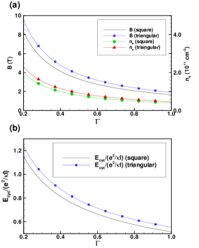
Figure 1: (Color online) Behaviour of (a) the magnetic field $B$ and electronic density $n_{e}$ and (b) the cyclotron energy ratio $E_{cyc}/(e^{2}/\kappa\ell)$ as a function of the parameter $\Gamma$ for the square and triangular lattices at filling factor $\nu=1$ and for a lattice constant of the external grid given by $a_{0}=50$ nm.

III HARTREE-FOCK HAMILTONIAN

The Hartree-Fock Hamiltonian of the interacting 2DEG in the presence of the grid is given by

$$H_{HF} = -N_{\varphi}\frac{\Delta_{Z}}{2}\sum_{\alpha}\sum_{n}E_{n}^{\alpha}\rho_{n,n}^{\alpha,\alpha}\left(0\right)$$

$$-\frac{eN_{\varphi}}{S}V_{g}\sum_{\mathbf{G}_{0}}\sum_{\alpha}\sum_{n_{1},n_{2}}F_{n_{1},n_{2}}\left(-\mathbf{G}_{0}\right)\rho_{n_{1},n_{2}}^{\alpha,\alpha}\left(\mathbf{G}_{0}\right)$$

$$+N_{\varphi}\frac{e^{2}}{\kappa\ell}\sum_{\alpha,\beta}\sum_{n_{1},...,n_{4}}\sum_{\mathbf{G}\neq 0}H_{n_{1},n_{2},n_{3},n_{4}}\left(\mathbf{G}\right)$$

$$\times\left\langle\rho_{n_{1},n_{2}}^{\alpha,\alpha}\left(-\mathbf{G}\right)\right\rangle\rho_{n_{3},n_{4}}^{\beta,\beta}\left(\mathbf{G}\right)$$

$$-N_{\varphi}\frac{e^{2}}{\kappa\ell}\sum_{\alpha,\beta}\sum_{n_{1},...,n_{4}}\sum_{\mathbf{q}}X_{n_{1},n_{4},n_{3},n_{2}}\left(\mathbf{G}\right)$$

$$\times\left\langle\rho_{n_{1},n_{2}}^{\alpha,\beta}\left(-\mathbf{G}\right)\right\rangle\rho_{n_{3},n_{4}}^{\beta,\alpha}\left(\mathbf{G}\right),$$

where $N_{\varphi}=S/2\pi\ell^{2}$ is the Landau level degeneracy with $S$ the 2DEG area. The variables $\alpha,\beta=\pm 1$ are spin indices while $n_{i}=0,1$ $\left(\text{with }i=1,2,3,4\right)$ are Landau level indices. The $\mathbf{G}=0$ Fourier component in the Hartree term is cancelled by the neutralizing positive background.

In Eq. (III), we have defined the operator

$$\rho_{n,m}^{\alpha,\beta}\left(\mathbf{G}\right) \equiv \frac{1}{N_{\varphi}}\sum_{X,X^{\prime}}e^{-\frac{i}{2}G_{x}\left(X+X^{\prime}\right)}$$

$$\times\delta_{X,X^{\prime}+G_{y}\ell^{2}}c_{n,X,\alpha}^{\dagger}c_{m,X^{\prime},\beta},$$

where $c_{n,X,\alpha}^{\dagger}$ creates an electron with guiding-center index $X$ (in the Landau gauge) with spin $\alpha$ in Landau level $n.$ These operators are related to the ground-state averaged electronic and spin densities by

$$n_{\alpha}\left(\mathbf{r}\right) = \frac{1}{2\pi\ell^{2}}\sum_{n_{1},n_{2}}\sum_{\mathbf{G}}F_{n_{1},n_{2}}\left(-\mathbf{G}\right)$$

$$\times\left\langle\rho_{n_{1},n_{2}}^{\alpha,\alpha}\left(\mathbf{G}\right)\right\rangle e^{i\mathbf{G}\cdot\mathbf{r}},$$

$$S_{\pm}\left(\mathbf{r}\right) = \frac{1}{2\pi\ell^{2}}\sum_{n_{1},n_{2}}\sum_{\mathbf{G}}F_{n_{1},n_{2}}\left(-\mathbf{G}\right)$$

$$\times\left\langle\rho_{n_{1},n_{2}}^{\pm,\mp}\left(\mathbf{G}\right)\right\rangle e^{i\mathbf{G}\cdot\mathbf{r}},$$

$$S_{z}\left(\mathbf{r}\right) = \frac{\hslash}{2}\left[n_{+}\left(\mathbf{r}\right)-n_{-}\left(\mathbf{r}\right)\right],$$ (14)

where $S_{\pm}=S_{x}\pm iS_{y}$. The form factors $F_{n_{1},n_{2}}\left(\mathbf{G}\right)$ are defined by

$$F_{n_{1},n_{2}}\left(\mathbf{G}\right) = \sqrt{\frac{\min\left(n_{1},n_{2}\right)!}{\max\left(n_{1},n_{2}\right)!}}L_{\min\left(n_{1},n_{2}\right)}^{\left|n_{1}-n_{2}\right|}\left(\frac{G^{2}\ell^{2}}{2}\right)$$

$$\times e^{-G^{2}\ell^{2}/4}\left(\frac{\left(\chi_{n_{1},n_{2}}G_{y}+iG_{x}\right)\ell}{\sqrt{2}}\right)^{\left|n_{1}-n_{2}\right|},$$

where $L_{n}^{m}\left(x\right)$ is a generalized Laguerre polynomial and $\chi_{n_{1},n_{2}}=$sgn$\left(n_{1}-n_{2}\right)$ with sgn the signum function. The dimensionless Hartree and Fock interactions are defined by

$$H_{n_{1},n_{2},n_{3},n_{4}}\left(\mathbf{G}\right) = \frac{1}{q\ell}F_{n_{1},n_{2}}\left(\mathbf{G}\right)F_{n_{3},n_{4}}\left(-\mathbf{G}\right),$$ (16)

$$X_{n_{1},n_{2},n_{3},n_{4}}\left(\mathbf{G}\right) = \int\frac{d\mathbf{p}\ell^{2}}{2\pi}\frac{1}{p\ell}F_{n_{1},n_{2}}\left(\mathbf{p}\right)$$

$$\times F_{n_{3},n_{4}}\left(-\mathbf{p}\right)e^{-i\widehat{\mathbf{z}}\cdot\left(\mathbf{p}\times\mathbf{G}\right)\ell^{2}}.$$

The averaged ”densities” $\left\{\left\langle\rho_{n,m}^{\alpha,\beta}\left(\mathbf{G}\right)\right\rangle\right\}$ are the order parameters that describe the various CDW or crystal states. They are computed by solving the Hartree-Fock equation for the single-particle Green’s function $G_{\alpha,\beta}\left(\mathbf{G,}\tau\right)$ defined by

$$G_{n,m}^{\alpha,\beta}\left(\mathbf{G,}\tau\right) = \frac{1}{N_{\varphi}}\sum_{X,X^{\prime}}e^{-\frac{i}{2}G_{x}\left(X+X^{\prime}\right)}$$

$$\times\delta_{X,X^{\prime}-G_{y}\ell^{2}}G_{n,m}^{\alpha,\beta}\left(X,X^{\prime},\tau\right),$$

where

$$G_{n,m}^{\alpha,\beta}\left(X,X^{\prime},\tau\right)=-\left\langle Tc_{n,X,\alpha}\left(\tau\right)c_{m,X^{\prime},\beta}^{\dagger}\left(0\right)\right\rangle.$$ (19)

The order parameters are obtained using the relation

$$\left\langle\rho_{n,m}^{\alpha,\beta}\left(\mathbf{G}\right)\right\rangle=G_{m,n}^{\beta,\alpha}\left(\mathbf{G,}\tau=0^{-}\right).$$ (20)

The equation of motion for $G_{n,m}^{\alpha,\beta}\left(\mathbf{G,}\omega_{n}\right)=\int_{0}^{\beta\hslash}d\tau e^{i\omega_{n}\tau}G\left(\mathbf{G},\tau\right),$ where $\omega_{n}=\left(2n+1\right)\pi/\beta\hslash$ with $\beta=1/k_{B}T$ is a fermionic Matsubara frequency, is a straightforward generalization of Eq. (14) of Paper 1 that includes two Landau levels instead of one. It leads to

$$\left[i\omega_{n}-\left(E_{m,\alpha}-\mu\right)/\hslash\right]G_{m,m^{\prime}}^{\alpha,\beta}\left(\mathbf{G},\omega_{n}\right)$$

$$= \delta_{\mathbf{G},0}\delta_{m,m^{\prime}}\delta_{\alpha,\beta}$$

$$-\frac{1}{\hslash S}\sum_{\mathbf{G}^{\prime}}\sum_{n}V_{g}\left(\mathbf{G}-\mathbf{G}^{\prime}\right)F_{m,n}\left(\mathbf{G}-\mathbf{G}^{\prime}\right)$$

$$\times\gamma_{\mathbf{G},\mathbf{G}^{\prime}}G_{n,m^{\prime}}^{\alpha,\beta}\left(\mathbf{G}^{\prime},\omega_{n}\right)$$

$$+\sum_{n}\sum_{\mathbf{G}^{\prime}\neq\mathbf{G}}U_{m,n}^{H}\left(\mathbf{G-G}^{\prime}\right)\gamma_{\mathbf{G},\mathbf{G}^{\prime}}G_{n,m^{\prime}}^{\alpha,\beta}\left(\mathbf{G}^{\prime},\omega_{n}\right)$$

$$-\sum_{n}\sum_{\gamma}\sum_{\mathbf{G}^{\prime}}\widetilde{U}_{m,n}^{F,\alpha,\gamma}\left(\mathbf{G-G}^{\prime}\right)\gamma_{\mathbf{G},\mathbf{G}^{\prime}}G_{n,m^{\prime}}^{\gamma,\beta}\left(\mathbf{G}^{\prime},\omega_{n}\right),$$

where $\gamma_{\mathbf{G},\mathbf{G}^{\prime}}=e^{-i\mathbf{G}\times\mathbf{G}^{\prime}\ell^{2}/2}$ and $n,m,m^{\prime}=0,1.$ The Hartree and Fock potentials are defined by

$$U_{m,n}^{H}\left(\mathbf{G}\right) = \left(\frac{e^{2}}{\hslash\kappa\ell}\right)\sum_{\gamma}\sum_{n_{1},n_{2}}H_{n_{1},n_{2},m,n}\left(-\mathbf{G}\right)$$

$$\times\left\langle\rho_{n_{1},n_{2}}^{\gamma,\gamma}\left(\mathbf{G}\right)\right\rangle,$$

$$\widetilde{U}_{m,n}^{F,\alpha,\gamma}\left(\mathbf{G}\right) = \left(\frac{e^{2}}{\hslash\kappa\ell}\right)\sum_{n_{1},n_{2}}X_{n_{1},n,m,n_{2}}\left(-\mathbf{G}\right)$$

$$\times\left\langle\rho_{n_{1},n_{2}}^{\gamma,\alpha}\left(\mathbf{G}\right)\right\rangle$$

and $n_{1},n_{2}=0,1.$

As described in Paper 1, the Hartree-Fock approximation leads to a set of $N_{\mathbf{G}}$ coupled and self-consistent equations where $N_{\mathbf{G}}$ is the number of RLVs kept in the calculation. This set of equations is solved numerically using an iterative method. Good convergence after $\approx 1000$ iterations is achieved by taking $N_{\mathbf{G}}\approx 600.$

Once the Green’s function is known, the density of states per area, $g\left(\omega\right),$ can be obtained from the relation

$$g\left(\omega\right)=-\frac{1}{2\pi^{2}\ell^{2}}\sum_{\alpha,n}\operatorname{Im}\left[G_{n,n}^{R,\alpha,\alpha}\left(\mathbf{G}=0,\omega\right)\right],$$ (24)

where $G_{n,n}^{R,\alpha,\alpha}\left(\mathbf{G}=0,\omega\right)$ is the retarded single-particle Green’s function obtained by the analytical continuation $G_{n,m}^{\alpha,\beta}\left(\mathbf{G,}i\omega_{n}\rightarrow\omega+i\delta\right)$ of the Matsubara Green’s function. The Hartree-Fock transport gap (at $T=0$ K) can be extracted directly from $g\left(\omega\right)$ since the Fermi level is fixed by the condition that $\nu=1.$

Note that the Hartree-Fock approach described here forces the CDW or crystal to be commensurate with the lattice potential. In Paper 1, however, we showed that a grid with a square unit cell of area $a_{0}^{2}$ could induce a crystal with a spin texture periodicity $\sqrt{2}a_{0}\times\sqrt{2}a_{0}$. In order to describe this state and keep the grid potential unchanged, we take the RLVs in the Hartree-Fock Hamiltonian of Eq. (III) to be given by: $\mathbf{G}=\frac{2\pi}{\sqrt{2}a_{0}}\left(n,m\right)$, with $n,m=0,\pm 1,\pm 2,...$ and take $\mathbf{G}_{0}$ in Eq. (2) to be on the second shell of these new RLV’s thus ensuring that $\left|\mathbf{G}_{0}\right|=2\pi/a_{0}$ is unchanged. We use a similar trick for the triangular grid, which, as we find in the present work, can induce a crystal with a spin texture periodicity $\sqrt{3}a_{0}\times\sqrt{3}a_{0}.$ In this case, the grid potential is unchanged if we take $\mathbf{G}_{0}$ to be on the third shell of the new RLV’s given by $\mathbf{G}=n\mathbf{G}_{1}+m\mathbf{G}_{2}$ where $n,m=0,\pm 1,\pm 2,...$ and $\mathbf{G}_{1}=\frac{2\pi}{\sqrt{3}a_{o}}\left(\frac{2}{\sqrt{3}},0\right),$ $\mathbf{G}_{2}=\frac{2\pi}{\sqrt{3}a_{o}}\left(\frac{1}{\sqrt{3}},1\right).$

IV PHASE DIAGRAM OF THE 2DEG FOR THE SQUARE GRID

We now derive the phase diagram of the 2DEG as a function of the potential strength $V_{g}$ [see Eq. (III)] for a square grid. We take $\nu=1$, $a_{0}=50$ nm and $\Gamma\in\left[0,1\right]$ including the two Landau levels $n=0,1.$ The phase diagram that we find is shown in Fig. 2. (Note that the lines connecting the $\Gamma$ points in this graph are merely a guide to the eyes and not a true phase boundary.) The numbers above the red symbols indicate the magnetic field $B$ in Tesla that corresponds to the corresponding value of $\Gamma.$

The phase diagram contains four phases. The electronic density is modulated spatially in all of them i.e. $n\left(\mathbf{r}\right)=n_{0}+\delta n\left(\mathbf{r}\right),$ where $n_{0}=1/2\pi\ell^{2}$ is the uniform density of a filled Landau level and $\delta n\left(\mathbf{r}\right)$ is the density modulation. The magnitude of the spin density is also modulated spatially and, for some phases, the orientation of the spins as well. The different phases are:

1. CDW1: a fully spin polarized CDW with all spins pointing in the direction of the external magnetic field. Both $n\left(\mathbf{r}\right)$ and $S_{z}\left(\mathbf{r}\right)$ have the periodicity $a_{0}\times a_{0}$ of the external potential. CDW1 is the ground state for $V_{g}\lesssim 2.0$ meV at all values of $\Gamma.$

2. VORTEX1: a CDW with a $\sqrt{2}a_{0}\times\sqrt{2}a_{0}$ magnetic unit cell. The density modulation is accompanied by a topological spin texture $\mathbf{S}\left(\mathbf{r}\right).$ The unit cell contains four spin vortices: two with a counterclockwise rotation (negative vorticity i.e. $n_{v}=-1$) and two with a clockwise rotation (positive vorticity i.e. $n_{v}=1$). The spin texture is similar to that shown in Fig. 4 of Paper 1 where only level $n=0$ was considered. The spin density $S_{z}\left(\mathbf{r}\right)$ is everywhere positive. Adjacent vortices with the same vorticity have the global phase of their spin texture rotated by $\pi$ with respect to one another. In a language where the global phase is mapped into an $xy-$spin, this $\pi$ rotation can be seen as an antiferromagnetic ordering of the vortex pair. The topological spin texture of this phase is reminiscent of that of the Skyrme crystal that occurs near $\nu=1$ in the absence of an external potentialFertigskyrme . The antiferromagnetic ordering keeps the spins as parallel as possible everywhere in space thus minimizing the exchange energy. The exchange energy is minimal when all spins are parallel, a situation realized in a quantum Hall ferromagnet.

3. VORTEX2: a phase similar to VORTEX1 with the same antiferromagnetic ordering but with the vorticity and sign of $S_{z}$ at each vortex core inverted. This phase is absent of the phase diagram for $\Gamma\geq 1/2.$

4. CDW2: a phase similar to CDW1 but only partially spin polarized with $\left\langle S_{z}\right\rangle=\left|\frac{1}{2}-\frac{\Gamma}{\varepsilon}\right|.$ There is no spin texture in this phase. The density modulations have larger amplitude than in CDW1 because of the stronger external potential.

The topological three-dimensional spin texture associated with each vortex is similar to that of a meron. In a meron, the spin points up or down at the core center and tilts away from the $\widehat{\mathbf{z}}$ direction away from the core. At large distance from the core, the spins point purely radially in the $x-y$ plane. For a meron core at $\mathbf{r}=0$ and for a field of unit spins, the topological charge $Q$ of a meron is defined by

$$Q=\frac{1}{2}\left[S_{z}\left(\infty\right)-S_{z}\left(0\right)\right]n_{v},$$ (25)

where $n_{v}$ is the vortex winding number (i.e. the number of $2\pi$ rotation around the vortex core)Moon . There are four flavors of meron and they all have half the topological charge of a skyrmion or antiskyrmion i.e. $\left|Q\right|=\frac{1}{2}.$ In this work, we associate a positive vorticity, $n_{v}=1,$ with a clockwise rotation of the spins. For $n_{v}=-1,$ a positive $S_{z}$ at the meron core is thus associated with a topological charge $Q=+1/2$ and, by the spin-charge coupling, with a positive density modulation (a local increase with respect to the uniform density i.e. $\delta n\left(\mathbf{r}\right)>0$). The opposite is true for $Q=-1/2$ i.e. $\delta n\left(\mathbf{r}\right)<0.$ Since no charge are added to the 2DEG which is kept at $\nu=1,$ there is an equal number of merons ($Q=+1/2$) and antimerons ($Q=-1/2$). We remark here that we use the word ”meron” in a loose sense since we are not really dealing with a classical field of unit spins but rather with a spin field that can be modulated both in orientation and in density. It follows that the charge in our ”merons” is not quantized. As $V_{g}$ is increased, $\delta n\left(\mathbf{r}\right)$ at the center of the vortices with positive density modulation becomes larger than $\delta n\left(\mathbf{r}\right)$ at the center of the vortex with negative modulation but $\int\delta n\left(\mathbf{r}\right)d\mathbf{r}=0.$

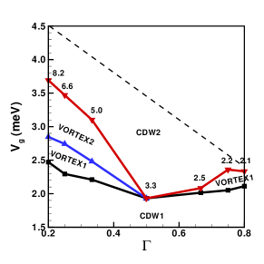
Figure 2: (Color online) Phase diagram of the 2DEG under a square superlattice potential $V_{g}$. The number above each red symbol gives the magnetic field (in Tesla) for that particular value of $\Gamma.$ Note that the lines are only a guide to the eye. Only the symbols correspond to calculated values. The dashed line indicates the upper limit in $V_{g}$ of our numerical calculation.

The addition of a second Landau level modifies the results reported in Paper 1. The most dramatic change is the disappearance of the uniform phase which was present before the VORTEX1 phase and its replacement by the CDW1 phase which now evolves continuously into the VORTEX1 state. The other two phase boundaries (VORTEX1-VORTEX2 and VORTEX2-CDW2) are only slightly modified by the addition of the second Landau level.

To evaluate the importance of the second Landau level, we compute the occupation of the four Landau levels as a function of the grid potential $V_{g}$. Figure 3 shows these occupations for $\Gamma=3/4$ where, according to Fig. 1, the Landau level mixing is expected to be the strongest. Our calculation shows that the mixing is small, but not negligible at that value of $\Gamma$. It varies very slightly with the grid potential in the range of values considered. The presence of the second Landau level is especially important at small value of $V_{g}$ where, as only $\nu_{0,\uparrow}$ and $\nu_{1,\uparrow}$ are nonzero, it allows for the formation of a non uniform state with no spin texture. As $V_{g}$ increases, the occupation of the $n=0,\alpha=\downarrow$ state more important than that of the $n=1,\alpha=\uparrow$ state. For $\Gamma<3/4,$ the occupation of the $n=1$ Landau level is much smaller than for $\Gamma=3/4.$ For example, it is $6\%$ at $\Gamma=1/2$ and $3.5\%$ at $\Gamma=1/4$ so that mixing is indeed small for small $\Gamma^{\prime}s.$

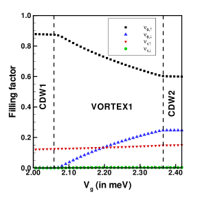
Figure 3: (Color online) Occupation (filling factor) of Landau levels $n=0,1$ with spin $\sigma=\pm 1$ as a function of the grid potential $V_{g}$ (in meV) for the square lattice at $\Gamma=3/4.$ The vertical dashed lines indicate the phase boundaries.

In the square lattice, the transition between the VORTEX1 and VORTEX2 phases for $\Gamma<1/2$ and between the VORTEX1 and CDW2 phases for $\Gamma>1/2$ is accompanied by a discontinuity in the spin component $S_{z}$ which we show in Fig. 4 for different values of $\Gamma$. The discontinuity increases with $\Gamma$ until it reaches a maximum (in absolute value) at $\Gamma=1/2$ where CDW1 is fully spin polarized while CDW2 is spin unpolarized. We found in Paper 1 that $\Delta S_{z}=0$ for the VORTEX1-CDW2 transition but this is no longer the case when Landau level $n=1$ is considered except when $\Gamma\geq 3/4.$ This discontinuity in $S_{z}$ should be detectable experimentally.

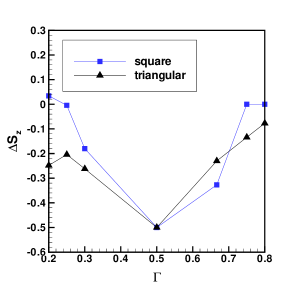
Figure 4: (Color online) Discontinuity in the $z$ component of the spin density as a function of $\Gamma$ for the square and triangular grids. For $\Gamma<1/2,$ the discontinuity is between the VORTEX1 and VORTEX2 phases for the square lattice and VORTEX3 and VORTEX4 for the triangular lattice while for $\Gamma>1/2$ it is between the VORTEX1 and CDW2 phases for the square lattice and between CDW1 and CDW2 for the triangular lattice.

V PHASE DIAGRAM FOR THE TRIANGULAR GRID

We now consider a triangular grid. The calculated phase diagram is shown in Fig. 5. As in Fig. 2, the symbols correspond to calculated values and the lines between them are guide to the eyes. The grid potential creates modulated states with a triangular lattice structure. Two phases: CDW1 and CDW2 are similar to the CDW’s of the square potential. They occupy the largest portion of the phase diagram. In between these two phases, we find two vortex phases which we name VORTEX3 (see Fig. 6) and VORTEX4 (see Fig. 7). They are present for $\Gamma<1/2$ only. In contrast with the square potential, they are not present if the Hilbert space is restricted to the Landau level $n=0$ only (in which case we find only two phases: a uniform phase, fully spin polarized and CDW2).

In the square lattice, we found that a pair of vortices (or merons) with the same vorticity prefer an antiferromagnetic ordering of the phase of their spin texture. In a triangular lattice, this type of interaction should lead to frustration and the expected ground state must have a three-sublattice structure with a $2\pi/3$ rotation of the phase from one meron to the other (with the same $Q$). This is indeed what we find in the VORTEX4 phase which is shown in Fig. 7. The magnetic unit cell is indicated by the parallelogram. This phase has 3 merons of positive (negative) vorticity at the each maximum (minimum) of the density. The spin component $S_{z}\left(\mathbf{r}\right)$ has not the same sign everywhere in space but is negative at the core of each meron whatever its vorticity. Vortices with $n_{v}=1$ thus correspond to density maxima (the red circles in Fig. 7) according to Eq. (25) and those with $n_{v}=-1$ to density minima (the large blue triangles in Fig. 7). The 3 merons with the same vorticity have the phase of their spin texture rotated by $2\pi/3$ from one another. They also have the same value of the local density modulation $\delta n\left(\mathbf{r}\right)$ in contrast with the VORTEX3 phase discussed below. Phase VORTEX4 is the analog of a three-sublattice antiferromagnet on a triangular lattice. As for the square lattice, maximal and minimal values of $\left|\delta n\left(\mathbf{r}\right)\right|$ are not equal but depend on $V_{g}.$ However, $\int\delta n\left(\mathbf{r}\right)d\mathbf{r}=0$ as no charge is added to the 2DEG.

The second vortex phase that we find, VORTEX3, is shown in Fig. 6. The magnetic unit cell is represented by the parallelogram. It contains 3 vortices with the same negative vorticity at the position of the density maxima. The spin component (not shown in Fig. 6) $S_{z}\left(\mathbf{r}\right)$ is positive everywhere so that the 3 vortices are associated with positive density modulations i.e. $\delta n\left(\mathbf{r}\right)>0$. The negative modulation is spread throughout the unit cell and not concentrated into antimerons. In contrast to VORTEX4, the 3 vortices in the unit cell do not share the same value of $\delta n\left(\mathbf{r}\right).$ One vortex has a larger value of $\delta n\left(\mathbf{r}\right)$ than the other two. Moreover, the spin texture of two of the three vortices have the same global while the phase of the third one is shifted by $\pi$ with respect to the other two. Considering the spin texture alone, VORTEX3 does not seem to resolve the frustration inherent to an antiferromagnetic coupling on a triangular lattice. We must keep in mind, however, that in our calculation both the orientation and the spin can change locally i.e. $\left|\mathbf{S}\left(\mathbf{r}\right)\right|$ is not uniform. In Fig. 6, vortices with the larger $\delta n\left(\mathbf{r}\right)$ are surrounded by $6$ neighbors of opposite phase thus optimizing the antiferromagnetic interaction. However, vortices with the smaller $\delta n\left(\mathbf{r}\right)$ are surrounded by 3 neighbors of opposite phase and 3 neighbors of the same phase. For them, the interaction is not optimal. In total, however, this seems to represent another way to resolve the frustration.

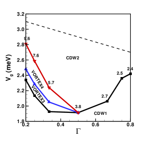
Figure 5: (Color online) Phase diagram of the 2DEG under a triangular superlattice potential $V_{g}$ (in meV). The number above each symbol gives the magnetic field (in Tesla) for that particular value of $\Gamma.$ Note that the lines connecting the symbols are only a guide to the eye. Only the symbols correspond to calculated values. The dashed line indicates the limit in $V_{g}$ of the numerical calculation.

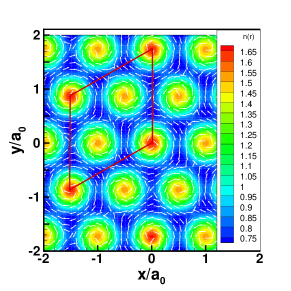
Figure 6: (Color online) Electronic density $n\left(\mathbf{r}\right)$ in units of $1/2\pi\ell^{2}$ and spin texture in the $x-y$ plane for the VORTEX3 state. Parameters: $\Gamma=1/4,a_{0}=50$ nm and $\nu=1.$ The magnetic unit cell is indicated by the parallelogram.

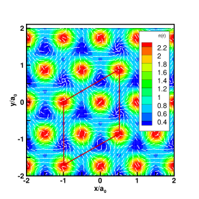
Figure 7: (Color online) Electronic density $n\left(\mathbf{r}\right)$ in units of $1/2\pi\ell^{2}$ and spin texture $\mathbf{S}\left(\mathbf{r}\right)$ in the $x-y$ plane for the VORTEX4 states. Parameters: $\Gamma=1/4,a_{0}=50$ nm and $\nu=1.$ The magnetic unit cell is indicated by the parallelogram.

We checked for the importance of Landau level mixing for the triangular grid. Our results are shown in Fig. 8 for the case $\Gamma=1/3.$ Clearly, the mixing is small at that value of $\Gamma$. But, for $\Gamma=4/5,$ the occupation of the $n=1$ Landau level reaches $20\%$ and mixing becomes significant as is the case for the square lattice. Figure 8 also clearly shows the discontinuous character of the transition from the VORTEX3 to the VORTEX4 phases.

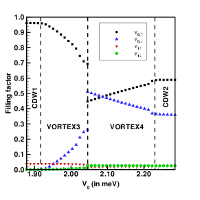
Figure 8: (Color online) Filling factor $\nu_{n,\sigma}$ of the four Landau levels $n=0,1$ with spin $\sigma=\pm 1$ as a function of the superlattice potential $V_{g}/\left(e^{2}/\kappa\ell\right)$ for the triangular lattice at $\Gamma=1/3.$ The vertical dashed lines indicate the boundaries of the different phases.

The transition between the VORTEX3 and VORTEX4 phases for $\Gamma<1/2$ or between the CDW1 and CDW2 phases for $\Gamma>1/2$ is accompanied by a discontinuity in $S_{z}$ which is plotted in Fig. 4. The behavior for the triangular lattice is similar to that of the square lattice. The decrease in $S_{z}$ is maximal (in absolute value) for $\Gamma=1/2$ where the transition is between the CDW1 (spin polarized) and CDW2 (spin unpolarized).

The VORTEX phases in the triangular lattice can also be distinguished from the behavior of their transport gap $\Delta_{eh}$ which is the energy to create an infinitely separated electron-hole pair. We evaluate this gap from the density of states given by Eq. (24). Figure 9 shows the dependency of $\Delta_{eh}$ on $V_{g}$ for $\Gamma=1/4.$ There is clear change in the slope of $\Delta_{eh}$ between VORTEX3 and VORTEX4 and between VORTEX4 and CDW2. The inset in Fig. 9 shows the density of states and the integrated density of states (blue line) in the VORTEX3 phase at $V_{g}=2.17$ meV. The maximum value of the integrated DOS is $4$ in the units of Fig. 9 corresponding to full occupation of the four states $n=0,1$ with $\sigma=\pm 1$. The gap is given by the size of the region where the integrated DOS is unity.

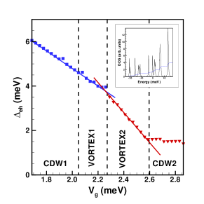
Figure 9: (Color online) Behavior of the Hartree-Fock gap $\Delta_{eh}$ as a function of the grid potential $V_{g}$ in the different phases of the triangular lattice at $\Gamma=1/4.$ The gap is evaluated from the density of states, an example of which is given in the inset for $V_{g}=2.17$ meV i.e. in the VORTEX3 phase. The blue line in the inset is the integrated density of states.

VI ELECTRIC DIPOLES

The averaged Fourier transform of the electronic density $n\left(\mathbf{G}\right)$ is related to the operator $\rho_{i,j}^{\alpha,\beta}\left(\mathbf{G}\right)$ introduced in Eq. (III) by the relation

$$n\left(\mathbf{G}\right)=N_{\varphi}\sum_{\alpha}\sum_{n,m}F_{n,m}\left(-\mathbf{G}\right)\left\langle\rho_{n,m}^{\alpha,\beta}\left(\mathbf{G}\right)\right\rangle.$$ (26)

For $n,m=0,1,$ Eq. (III) gives for the form factors:

$$F_{0,0}\left(\mathbf{G}\right) = e^{-G^{2}\ell^{2}/4},$$ (27)

$$F_{1,1}\left(\mathbf{G}\right) = \left(1-\frac{G^{2}\ell^{2}}{2}\right)e^{-G^{2}\ell^{2}/4},$$ (28)

$$F_{1,0}\left(\mathbf{G}\right) = \left(\frac{\left(G_{y}+iG_{x}\right)\ell}{\sqrt{2}}\right)e^{-G^{2}\ell^{2}/4},$$ (29)

$$F_{0,1}\left(\mathbf{G}\right) = \left(\frac{\left(-G_{y}+iG_{x}\right)\ell}{\sqrt{2}}\right)e^{-G^{2}\ell^{2}/4}.$$ (30)

If we use a pseudospin language where index $0$ is for orbital $n=0$ and $1$ for orbital $n=1,$ then the electronic and spin densities are given by

$$\rho^{\alpha}\left(\mathbf{G}\right) = \rho_{0,0}^{\alpha,\alpha}\left(\mathbf{G}\right)+\rho_{1,1}^{\alpha,\alpha}\left(\mathbf{G}\right),$$ (31)

$$\rho_{z}^{\alpha}\left(\mathbf{G}\right) = \left(\rho_{0,0}^{\alpha,\alpha}\left(\mathbf{G}\right)-\rho_{1,1}^{\alpha,\alpha}\left(\mathbf{G}\right)\right)/2,$$ (32)

$$\rho_{0,1}^{\alpha,\alpha}\left(\mathbf{G}\right) = \rho_{x}^{\alpha}\left(\mathbf{G}\right)+i\rho_{y}^{\alpha}\left(\mathbf{G}\right),$$ (33)

$$\rho_{1,0}^{\alpha,\alpha}\left(\mathbf{G}\right) = \rho_{x}^{\alpha}\left(\mathbf{G}\right)-i\rho_{y}^{\alpha}\left(\mathbf{G}\right).$$ (34)

It follows that

$$n\left(\mathbf{G}\right) = N_{\varphi}\sum_{\alpha}\left(1-\frac{G^{2}\ell^{2}}{4}\right)\left\langle\rho^{\alpha}\left(\mathbf{G}\right)\right\rangle e^{-G^{2}\ell^{2}/4}$$

$$+N_{\varphi}\sum_{\alpha}\left(\frac{G^{2}\ell^{2}}{2}\right)\left\langle\rho_{z}^{\alpha}\left(\mathbf{G}\right)\right\rangle e^{-G^{2}\ell^{2}/4}$$

$$-N_{\varphi}\sqrt{2}i\sum_{\alpha}\left[G_{x}\ell\left\langle\rho_{x}^{\alpha}\left(\mathbf{G}\right)\right\rangle-G_{y}\ell\left\langle\rho_{y}^{\alpha}\left(\mathbf{G}\right)\right\rangle\right]$$

$$\times e^{-G^{2}\ell^{2}/4}.$$

In this pseudospin language, the averaged coupling of the 2DEG with the grid potential is written as

$$\left\langle W\right\rangle = -\frac{eN_{\varphi}}{S}\sum_{\alpha}\sum_{n,m}\sum_{\mathbf{G}}V_{e}\left(-\mathbf{G}\right)F_{n,m}\left(-\mathbf{G}\right)$$

$$\times\left\langle\rho_{n,m}^{\alpha,\alpha}\left(\mathbf{G}\right)\right\rangle$$

$$= -\frac{eN_{\varphi}}{S}\sum_{\alpha}\sum_{\mathbf{G}}V_{e}\left(-\mathbf{G}\right)\left(1-\frac{G^{2}\ell^{2}}{4}\right)\left\langle\overline{\rho}^{\alpha}\left(\mathbf{G}\right)\right\rangle$$

$$-\frac{eN_{\varphi}}{S}\sum_{\alpha}\sum_{\mathbf{G}}V_{e}\left(-\mathbf{G}\right)\left(\frac{q^{2}\ell^{2}}{2}\right)\left\langle\overline{\rho}_{z}^{\alpha}\left(\mathbf{G}\right)\right\rangle$$

$$+\frac{eN_{\varphi}}{S}\sqrt{2}i\sum_{\alpha}\sum_{\mathbf{G}}V_{e}\left(-\mathbf{G}\right)$$

$$\times\left[q_{x}\ell\left\langle\overline{\rho}_{x}^{\alpha}\left(\mathbf{G}\right)\right\rangle-q_{y}\ell\left\langle\overline{\rho}_{y}^{\alpha}\left(\mathbf{G}\right)\right\rangle\right]$$

where we have defined

$$\overline{\rho}_{i}^{\alpha}\left(\mathbf{G}\right)=\rho_{i}^{\alpha}\left(\mathbf{G}\right)e^{-G^{2}\ell^{2}/4}.$$ (37)

The electric field $\mathbf{E}_{\|}\left(\mathbf{r}\right)$ in the plane of the 2DEG is given by

$$\mathbf{E}_{\|}\left(\mathbf{r}\right)=-\nabla V_{e}\left(\mathbf{r}\right)=-\frac{1}{S}\sum_{\mathbf{G}}i\mathbf{G}V_{g}\left(\mathbf{G}\right)e^{i\mathbf{G}\cdot\mathbf{r}},$$ (38)

and

$$\mathbf{\nabla}_{\|}\cdot\mathbf{E}_{\|}\left(\mathbf{r}\right)=\frac{1}{S}\sum_{\mathbf{G}}G^{2}V_{g}\left(\mathbf{G}\right)e^{i\mathbf{G}\cdot\mathbf{r}}.$$ (39)

In real space, Eq. (VI) becomes

$$\left\langle W\right\rangle = -eN_{\varphi}\sum_{\alpha}\int d\mathbf{r}\left\langle\overline{\rho}^{\alpha}\left(\mathbf{r}\right)\right\rangle V_{g}\left(\mathbf{r}\right)$$

$$+\frac{1}{2}\ell^{2}eN_{\varphi}\sum_{\alpha}\int d\mathbf{r}\left\langle\overline{\rho}_{1,1}^{\alpha}\left(\mathbf{r}\right)\right\rangle\mathbf{\nabla}_{\|}\cdot\mathbf{E}_{\|}\left(\mathbf{r}\right)$$

$$+\sqrt{2}\ell eN_{\varphi}\sum_{\alpha}$$

$$\times\int d\mathbf{r}\left[\left\langle\overline{\rho}_{x}^{\alpha}\left(\mathbf{r}\right)\right\rangle E_{x}\left(\mathbf{r}\right)-\left\langle\overline{\rho}_{y}^{\alpha}\left(\mathbf{r}\right)\right\rangle E_{y}\left(\mathbf{r}\right)\right].$$

The third line in this equation can be written as a coupling between a dipole density and the electric field in the plane of the 2DEG, i.e.:

$$\left\langle W\right\rangle_{dipole}=-\int d\mathbf{rd}\left(\mathbf{r}\right)\cdot\mathbf{E}_{\|}\left(\mathbf{r}\right),$$ (41)

if we define

$$\mathbf{d}\left(\mathbf{G}\right) = -e\sqrt{2}\ell N_{\varphi}\sum_{\alpha}\left(\left\langle\overline{\rho}_{x}^{\alpha}\left(\mathbf{G}\right)\right\rangle\widehat{\mathbf{x}}-\left\langle\overline{\rho}_{y}^{\alpha}\left(\mathbf{G}\right)\right\rangle\widehat{\mathbf{y}}\right),$$ (42)

$$\mathbf{d}\left(\mathbf{r}\right) = \frac{1}{S}\sum_{\mathbf{G}}\mathbf{d}\left(\mathbf{G}\right)e^{i\mathbf{G}\cdot\mathbf{r}}.$$ (43)

The superposition of the $n=0$ and $n=1$ orbital states can thus be viewed as creating a density of electric dipoles $\mathbf{d}\left(\mathbf{r}\right)$ShizuyaED . Figure 10 shows the electronic density and dipole texture for the VORTEX1 phase at $V_{g}/\left(e^{2}/\kappa\ell\right)=0.22$ for the square lattice with $\Gamma=1/4.$ The dipole texture on each lattice site is qualitatively the same for all phases (CDW’s and VORTEX’s). In fact, the dipole field is basically that of the vector field $\mathbf{E}_{\|}\left(\mathbf{r}\right)$ in the plane of the 2DEG. The electric dipoles align themselves with the external potential of the grid. In contrast with the spin field $\mathbf{S}\left(\mathbf{r}\right)$ which is topologically different between the CDW’s and VORTEX’s phases, it does not seem possible to distinguish between the different phases from their dipole texture alone.

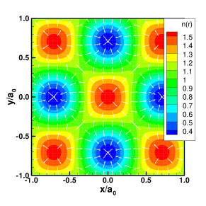
Figure 10: (Color online) Electronic density $n\left(\mathbf{r}\right)$ and dipole field $\mathbf{d}\left(\mathbf{r}\right)$ in the $x-y$ plane for the VORTEX1 phase at $V_{g}/\left(e^{2}/\kappa\ell\right)=0.22$ for the square lattice with parameters $a_{0}=50$ nm, $\Gamma=1/4$ and $\nu=1.$

VII CONCLUSION

It appears from the numerical results that we have presented in this paper, that the phase diagram of the 2DEG in a square lateral superlattice potential is not radically modified by the inclusion of a second Landau level in the Hartree-Fock equation of motion. The main result is the replacement of the uniform phase found in Paper 1 by a phase with density modulation but no spin texture. As expected, the occupation of the $n=1$ Landau level increases with $\Gamma$ since a higher value of $\Gamma$ means a smaller magnetic field i.e. more Landau level mixing.

For a triangular superlattice potential, a case not considered in Paper1, the phase diagram is enriched by the introduction of the $n=1$ Landau level. Apart from two CDW states with no spin modulation, we find vortex phases analog to that found for the square superlattice. In particular, the VORTEX4 phase has the three-sublattice structure expected for a lattice of merons where two adjacent merons with the same vorticity prefer to have the global phase associated with their spin texture differing by a phase $\pi.$ As for an antiferromagnet on a triangular lattice, the spin frustration that this interaction create is resolved by having adjacent spins rotated by $120$ degrees leading to a three-sublattice antiferromagnet. The VORTEX3 phase which occurs just before VORTEX4 seems to resolve the inherent frustration of an antiferromagnetic ordering on a triangular lattice by having unequal density for the three merons.

In Paper1, we calculated the collective mode dispersion of the different phases of the square lattice in the generalized random-phase approximation (GRPA). We showed that the VORTEX1 and VORTEX2 phases have an additional Goldstone mode that is related to their spin texture, the Hartree-Fock energy being independent of the global phase of the spin texture as is the case in a Skyrme crystalCoteGirvin . We expect that a similar Goldstone mode should be present for the triangular superlattice, at least for the VORTEX4 phase. Calculating the dispersion relation of the collective modes is one way to ascertain the stability of a phase and it would be interesting to be able to do it for the VORTEX3 state. When the $n=1$ Landau level is considered, however, the size of the matrices involved in the GRPA calculation are of the order of $16N_{\mathbf{G}}\times 16N_{\mathbf{G}}$ where $N_{\mathbf{G}}\approx 600$ is the number of reciprocal lattice vectors needed to described the vortex lattices. Those are too big matrices to diagonalize with our current computational resources.

References

• (1) R. Côté and Xavier Bazier-Matte, Phys. Rev. B 94, 205303 (2016).
• (2) For an early review of this problem, see for example: Daniela Pfannkuche and Rolf R. Gerhardts, Phys. Rev. B 46, 12606 (1992).
• (3) A. Rauh, Phys. Status Solidi B 65, K131 (1974); A. Rauh, Phys. Status Solidi B 69, K9 (1975); R. R. Gerhardts, D. Weiss, and K. v. Klitzing, Phys. Rev. Lett. 62, 1173 (1989); R. W. Winkler, J. P.. Kotthaus and K. Ploog, Phys. Rev. Lett. 62, 1177 (1989); Vidar Gudmundsson and Rolf R. Gerhardts, Phys. Ref. B 52, 16744 (1995).
• (4) D. R. Hofstadter, Phys. Rev. B 14, 2239 (1976).
• (5) B. Hunt, J. D. Sanchez-Yamagishi, A. F. Young, M. Yankowitz, B. J. LeRoy, K. Watanabe,T. Taniguchi, P. Moon, M. Koshino, P. Jarillo-Herrero, R. C. Ashoori, Science 340, 1427 (2013); Till Schlösser, Klaus Ensslin, Jörg P. Kotthaus and Martin Holland, Semicond. Sci. Technol. 11, 1582 (1996); C. R. Dean, L. Wang, P. Maher, C. Forsythe, F. Ghahari, Y. Gao, J. Katoch, M. Ishigami, P. Moon, M. Koshino, T. Taniguchi, K.Watanabe, K. L. Shepard, J. Hone and P. Kim, Nature 497, 598 (2013); C. Albrecht, J. H. Smet, K. von Klitzing, D. Weiss, V. Umansky, and H. Schweizer, Phys. Rev. Lett. 86, 147 (2001); T. Schloesser, K. Ensslin, J. P. Kotthaus, and M. Holland, Europhys. Lett. 33, 683 (1996); Cheol-Hwan Park and Steven G. Louie, Nano Letters 9, 1793 (2009); R. R. Gerhardts, D. Weiss, and U. Wulf, Phys. Rev. B 43, 5192 (1991).
• (6) Wenchen Luo and Tapash Chakraborty, J. Phys.: Condens. Matter 28, 0158801 (2016).
• (7) V. M. Apalkov and T. Chakraborty, Phys. Rev. Lett. 112, 176401 (2014); Areg Ghazaryan and Tapash Chakraborty, Phys. Rev. B 91, 125131 (2015).
• (8) Godfrey Gumbs and Paula Fekete, Phys. Rev. B 56, 3787 (1997).
• (9) Marco Gibertini, Achintya Singha, Vittorio Pellegrini, Marco Polini, Giovanni Vignale and Aron Pinczuk, Phys. Rev. B 79, 241406(R) (2009).
• (10) S. Melinte, Mona Berciu, Chenggang Zhou, E. Tutuc, S. J. Papadakis, C. Harrison, E. P. De Poortere, Mingshaw Wu, P.M. Chaikin, M. Shayegan, R.N. Bhatt, and R.A. Register, Phys. Rev. Lett. 92, 036802 (2004).
• (11) K. Moon, H. Mori, Kun Yang, S. M. Girvin, A. H. MacDonald, L. Zheng, D. Yoshioka, and Shou-Cheng Zhang, Phys. Rev. B 51, 5138 (1995).
• (12) For a review, see The quantum Hall Effect, edited by R. E. Prange and S. M. Girvin (Springer-Verlag, New York, 1990) and also the lecture notes of M. O. Goerbig, arXiv:0909.1998.
• (13) For a review on skyrmions, see Z. F. Ezawa, Quantum Hall Effects (World Scientific, Singapore, 2000) or S. M. Girvin and A. H. MacDonald in Perspectives in Quantum Hall Effects, edited by S. Das Sarma and A. Pinczuk (Wiley, New York, 1997).
• (14) R. Côté, H. A. MacDonald, Luis Brey, H. A. Fertig, S. M. Girvin and H. T. C. Stoof, Phys. Rev. Lett. 78, 4825 (1997).
• (15) L. Brey, H. A. Fertig, R. Côté, and A. H. MacDonald, Phys. Rev. Lett. 75, 2562 (1995).
• (16) K. Shizuya, Phys. Rev. B79, 165402 (2009).