Abstract

This thesis employs statistical learning technique to analyze, predict and solve the fixed charge network flow (FCNF) problem, which is common encountered in many real-world network problems. The cost structure for flows in the FCNF involves both fixed and variable costs. The FCNF problem is modeled mixed binary linear programs and can be solved with standard commercial solvers, which use branch and bound algorithm. This problem is important for its widely applications and solving challenges. There does not exist a efficient algorithm to solve this problem optimally due to lacking tight bounds.

To the best of our knowledge, this is the first work that employs statistical learning technique to analyze the optimal flow of the FCNF problem. Most algorithms developed to solve the FCNF problem are based on the cost structure, relaxation, etc. We start from the network characteristics and explore the relationship between properties of nodes, arcs and networks and the optimal flow. This is a bi-direction approach and the findings can be used to locate the features that affect the optimal flow most significantly, predict the optimal arcs and provide information to solve the FCNF problem.

In particular, we define 33 features based on the network characteristics, from which using step wise regression, we identify 26 statistical significant predictors for logistic regression to predict which arcs will have positive flow in the optimal solutions. The predictive model achieves $88\%$ accuracy and the area under receiver operating characteristic curve is $0.95$. Two applications are investigated. Firstly, the predictive results can be used directly as component critical index. The failure of arcs with higher critical index result in more cost increase over the entire network. Specifically, in the $100$ instances, total cost has an average of $9.8\%$ increase while blocking highest two critical arcs. Secondly, we develop a regression-based relaxation (RBR) solution approach to the FCNF problem, in which the variable costs are replaced by a function of predictive probability. The rigorous experiments demonstrate the efficacy of the RBR by outperforming linear programming and state-of-the-art standard exact technique.

Chapter 1 Introduction

1.1 Fixed Charge Network Flow Problem

The fixed charge network flow problem (FCNF) was first developed by Hirsch and Dantzig [29], which can be easily described as follows. For a given network, each node has supply/demand request and all the arcs between nodes have variable and fixed costs. The aim of the FCNF is to select the arcs and assign flow on them to transfer commodities from supply nodes to demand nodes, such that the total cost is minimum. Many practical problems, such like transportation problem [3, 22], lot sizing problem [49], facility location problem [41], network design [33, 27, 14] and others [30, 2, 37, 56, 58, 40, 61, 54, 55, 59, 60, 57] can be modeled as the FCNF.

The FCNF is NP-hard [26] and over the decades, a significant number of papers have been published providing solution approaches to the FCNF. In 1966, Driebeek [21] proposed an algorithm to solve a mixed integer problem, which contains a large number of continuous variables and a few integer variables. He solved the problem without integer constraints first and search for the optimum integer solution. This work was among the pioneers of mixed integer programming. Many techniques commonly utilities branch and bound (B&B) to search the exact solution of the FCNF. Kennington and Unger [31] presented a new branch and bound algorithm to fixed charge transportation problem, which exploited the underlying transportation structure. Barr et al. [5] revised B&B to solve large scale and sparse fixed charge transportation problem. Cabot and Erenguc [11] discussed three properties that may improve B&B algorithm. Palekar et al. [44] developed a stronger conditional penalty for the FCNF problem, which reduced the B&B enumeration and solving time significantly. Ortega and Wolsey [43] developed branch and cut system for uncapacitated FCNF problem, including a heuristic for the dicut inequalities and branching and pruning rules. Hewitt et al. [28] obtained better solution using careful neighborhood search from arc-based formulation of the FCNF and improved the lower bound by linear relaxation of the path-based formulation.

Due to lacking the tight upper and lower bounds, the B&B algorithm might be computational difficulty for the large-scale and complex problems. Hence, approximate solution approaches to find the near-optimal solution for the FCNF have generated considerable research interests. Balinski [3] formulated fixed cost transportation problem as integer programming and proposed a approximate method of solution. Sun et al. [50] applied Tabu search algorithm to solve the FCNF problem, using recency based and frequency based memories, intermediate and long term memory processes. For local search, they used network simplex method. Kim and Pardalos [32] developed a dynamic slope scaling procedure, incorporating variable and fixed costs together as a new coefficient and solve linear programming problem iteratively. Monteiro et al. [38] proposed a hybrid ant colony optimization algorithm to combine two aspects of meta-heuristic search behavior, exploration and exploitation. Based on spanning tree and Prüfer number representation, Molla-Alizadeh-Zavardehi et al. [37] proposed an artificial immune algorithm and genetic algorithm and discussed the proper values of parameters.

State-of-the-art MIP solvers combine a variety of cutting plane techniques, heuristics and the branch and bound algorithm to find the global optimal solution. All the modern MIP solvers use preprocessing/pre-solve methods to find a better upper bound by taking information from the original formulations, then the solvers are able to reduce the search space during B&B procedure, which significantly accelerate the entire solving processes [9]. More details of the preprocessing techniques can be found in the books of Nemhauser and Wolsey [39], Wolsey [52], Fügenschuh and Martin [25] and Mahajan [35].

1.2 Identification of Critical Components

Modern societies are heavily dependent on many distributed systems, e.g. communication networks [13], electric power transmission networks [20], transportation networks [62], and all these belongs to network science area. A substantial body of work has been done to identify critical components of networks. In general,the removal or blockage of one or more critical links could have direct and serious economic consequences in terms of overall system performance [6, 47]. Therefore, we need to identify critical segments in the network, as specified by several national and transnational directives [8]. The definition of criticality is always associated with a metric, such as travel time, maximum traffic flow, reliability and resilience, etc and the failure of critical components affect the system performance most. The term ’criticality’ is used to qualify the role that the elements play with respect to the global properties of the whole network.

Many literature employed topological approach to identify critical components, which is capable of identifying the network edges and nodes whose failure can induce a severe structural damage to the network through the physical disconnection of its parts [16, 10]. However, focusing on network topology neglects other characteristics of the network. Eusgeld et al. [23] employed simulation technique to capture the dynamics of the operational scenarios involving the most vulnerable parts of the critical infrastructure combined with the analysis of network topology. Bier et al. [7] proposed a computational efficient greedy algorithm, named max line interdiction algorithm, to identify the highest load line in the power system. Dheenadayalu et al. [19] identified critical highway links using localized level-of-service measures such as the volume/capacity (V/C) ratio. Scott et al. [45] developed a comprehensive Network Robustness Index for identifying critical components and network performance considering traffic flow, capacity and network connectivity. Through hypothetical networks, they proved that the Network Robustness Index yields different greater system-wide benefits with respect to travel time savings, than solution identified by V/C ratio.

Besides network analysis and simulation approach, optimization is widely to identify critical components. Zio et al. [63] proposed a multi-objective optimization model aimed at the maximization of the importance of the importance of the groups and minimization of their dimension. They applied the model to analyze the Italian high-voltage electrical transmission network. Similarly, Shen et al. [46] developed three objectives including the maximization of the number of connected components, minimization of the largest component size and maximization of the minimum cost required to reconnect the whole network, by deleting a group of nodes.

In addition, Demšar et al. [18] proposed a dual graph model to identify critical locations in a spatial network in terms of vulnerability risk. Crucitti et al. [15] proved that the disruption of a single critical node is sufficient to decrease the efficiency or performance of the entire system. Barker et al. [4] involves two critical importance measures considering the adverse impact while blocking the link and positive impact if the link is not disrupted in the disaster.

In summary, the critical index can be built in terms of different scenarios. Removing the network component and quantifying the corresponding system-wide consequence is widely employed to build the component importance index regardless which technique used in the literature.

1.3 Principal Goals and Thesis Outlines

As the best of our knowledge, none of existing literature have developed models to analyze and predict which arcs are used in the optimal solution of the FCNF. This is the first paper that employs statistical learning technique to analyze the optimal flow of the FCNF and distinguishes the features to predict the optimal arcs. This thesis involves three tasks. Task 1 will extract network features that can be used as predictors and how to develop a predictive model with these features. By solving thousands of random generated FCNF instances, we collect over $60,000$ observations and develop logistic regression model based on the dataset, which can be used to quantify the influence of each statistical significant network characteristics. Task 2 will validate the predictive model through a series of diagnostic techniques will interpret the model. Task 3 of this thesis, will discuss two applications of this model. The first one is to identify critical arcs in a network with respect to the FCNF problem without solving any optimization problems. The other one is named regression-based relaxation (RBR), a approximate method for the FCNF.

The remainder of this thesis is organized as follows. Chapter 2 introduces the background of the FCNF and the logistic regression model. The whole process for developing logistic regression model is discussed in Chapter 3 and Chapter 4 validates and interprets the predictive model. Chapter 5 introduces two applications of the predictive model. Chapter 6 and 7 summarize the thesis and future work, respectively.

Chapter 2 Background

2.1 Fixed Charge Network Flow Formulation

The fixed charge network flow (FCNF) problem is described on a network $G=(N,A)$, where $N$ and $A$ are the set of node index $i$ and arc index $(i,j)$, respectively. Let $c_{ij}$ and $f_{ij}$ denote the variable and fixed cost of arc $(i,j)\in A$, respectively. Each node has a supply/demand request $R_{i}$ ($R_{i}>0$ if node $i$ is a supply node; $R_{i}<0$ if node $i$ is a demand node; otherwise, $R_{i}=0$). Artificial capacity, $M_{ij}$, is used in the problem formulation to ensure that the fixed cost $f_{ij}$ is incurred whenever there is a positive flow on arc $(i,j)\in A$. There are two variables in the FCNF, $x_{ij}$ denotes the flow and $y_{ij}$ represents the corresponding decision variable on arc $(i,j)\in A$ . All the instances in this work are single-commodity FCNF and the formulation is as follows,

min $$\sum_{(i,j)\in A}(c_{ij}x_{ij}+f_{ij}y_{ij})$$ (2.1)

s.t. $$\sum_{(i,j)\in A}x_{ij}-\sum_{(j,i)\in A}x_{ji}=R_{i} \forall{i\in N}$$ (2.2)

$$0\leq x_{ij}\leq M_{ij}y_{ij} \forall{(i,j)\in A}$$ (2.3)

$$y_{ij}\in\{0,1\} \forall{(i,j)\in A}$$ (2.4)

Here, the objective function in (2.1) is nonlinear. Constraint (2.2) ensures that the inflow and outflow satisfy the supply/demand at node $i\in N$. $M_{i,j}$ is arc capacity in constraint (2.3) to ensure that the flow on arc $(i,j)\in A$ can be positive only when the arc $(i,j)\in A$ is open ($y_{ij}=1$). If arc$(i,j)$ is not capacitated, $M_{ij}$ should be artificially set to a number which is larger than the total supply requests to not inhibit feasible solution. Constraint (2.4) defines $y_{ij}$ as binary, which makes the problem a 0-1 mixed integer programming problem.

2.2 Logistic Regression Model

The logistic regression is a classification model and only has one response/dependent variable. The logistic regression is commonly used in data mining applications, computer science, biology and so on [12]. There are two classes of the logistic regression, binomial and multinomial. The response variable of binomial logistic regression has exactly two classes or binary outcomes, while multinomial logistic regression has more than two. The dependent variable in this paper, denoted by $Y$, is binary and

$$Y=\begin{cases}1,\text{arc is used in the FCNF}\\ 0,\text{otherwise}.\end{cases}$$

The initial output of the logistic regression is not $0$ or $1$, but the probability that the response variable equals to $1$, which in this work refers to the likelihood that the arc has positive flow in the optimal solution of the FCNF. The probability is derived by a logistic function of a variety of independent predictors and the logistic regression coefficients. We use $\pi(p)=P(Y=1|p_{1},p_{2},\dots,p_{k},\dots,p_{K})$ to represent the conditional probability of $Y=1$ given $p_{k}$ when the logistic regression is used. The specific logistic regression model is,

$$\pi(p)=\dfrac{1}{1+e^{-(\beta_{0}+\beta_{1}p_{1}+\beta_{2}p_{2}+\dots+\beta_{k}p_{k}+\dots+\beta_{K}p_{K})}}$$ (2.5)

where $K$ is the total number of independent predictors, $p_{k}$ is the $k^{\text{k}}$ predictor and $\beta_{k}$ is the $k^{\text{th}}$ parameter. Let $g(p)$ denote the logistic transformation of $\pi(p)$ and defined as,

$$g(p) =ln[\dfrac{\pi(p)}{1-\pi(p)}]$$

$$=\beta_{0}+\beta_{1}p_{1}+\beta_{2}p_{2}+\dots+\beta_{k}p_{k}+\dots+\beta_{K}p_{K}$$

The logit, $g(p)$, is linear in its parameters. The logistic transformation has many desirable properties of linear regression which we will use to discuss the model and interpretation. Transforming the likelihood to binary value needs a cut-off point, above which the response variable is set to $1$. The details of setting the cut-off value is discussed in Chapter 4.

Chapter 3 Optimal Flow Analysis

3.1 Network Features Extraction

In this section, we extract features from network to predict which arcs will be open in the optimal solutions of the FCNF with four types of features (network, arcs, relaxation solutions and nodes). In the network level, the features include the total number of nodes ($n$), the number of arcs ($m$), the sum of supply requests ($S$) and the density of network , which is denoted by $\rho=\frac{m}{2\binom{n}{2}}$. The total supplies is transformed to the average supply per node, $\bar{S}=\frac{S}{n}$. Arc $(i,j)\in A$ has variable cost $c_{ij}$ and fixed cost $f_{ij}$ based on formulation (2.1). Let $\gamma_{ij}$ denote the ratio between fixed cost and variable cost of arc $(i,j)\in A$,

$$\gamma_{ij}=\frac{f_{ij}}{c_{ij}}\qquad\forall{(i,j)\in A}.$$

Let $l_{ij}$ denote the flow solution of arc $(i,j)\in A$ in linear relaxed FCNF problem and the normalized value of $l_{ij}$ is denoted by $\bar{l}_{ij}$,

$$\bar{l}_{ij}=\frac{l_{ij}}{S}\qquad\forall(i,j)\in A.$$

The value of $\bar{l}_{ij}$ indicates the optimal flow of the linearized FCNF, and another binary predictor of the optimal arc is created, which is denoted by $l^{B}_{ij}$,

$$l^{B}_{ij}=\begin{cases}1,\bar{l}_{ij}>0\\ 0,\text{otherwise}.\end{cases}$$

The two predictors are both related with the optimal flow in the linear relaxed FCNF, but reflect two different types of information. The value of $\bar{l}_{ij}$ indicates how much flow on arc $(i,j)\in A$ and $l^{B}_{ij}$ shows the arc is open or not in the linearized FCNF.

The information of head node $i$ and tail node $j$ of arc $(i,j)\in A$ should also be considered as the features that may facilitate the predictive model due to the fact that the goal of FCNF is to transfer commodities from supply nodes to demand nodes through several transshipment nodes. Accordingly, we detail the predictors associated with head node $i\in N$, with which tail node $j\in N$ is same. Let $t_{i}$ denote the type of node $i\in N$,

$$t_{i}=\begin{cases}1,r_{i}>0\\ 0,r_{i}=0\\ -1,r_{i}<0\end{cases}.$$

This is to say if node $i$ is a supply node, $t_{i}=1$; if node $i$ is a transshipment node, $t_{i}=0$ ; and otherwise if node $i$ is a demand node, $t_{i}=-1$. Let $d_{i*}$ denote the outdegree of node $i$. It is reasonable to assume that the nodes adjacent to node $i$ have a significant influence on the corresponding response variable. For example, if a supply node is connected with node $i$, the probabilities of this arc and other arcs out from node $i$ to be selected will increase. Let $d_{i*}^{S}$ ($d_{i*}^{D}$) denote the number of supply (demand) tail nodes adjacent to node $i$. If a demand node is connected with node $i$, the probabilities of this arc and other arcs into node $i$ to be selected will increase as well. Let $r_{i*}^{S}$ ($r_{i*}^{D}$) denote the sum of supply (demand) requirements of the tail endpoints adjacent to node $i$. In the same way, the indegree of node $i$ is denoted as $d_{*i}$, the number of supply (demand) head nodes adjacent to node $i$ is denoted by $d_{*i}^{S}$ ($d_{*i}^{D}$), and sum of supply (demand) requests of head endpoints adjacent to node $i$ are denoted as $r_{*i}^{S}$ ($r_{*i}^{D}$). Figure 3.1 illustrates the notations with a small directed network, in which the number under each node is the requirements of that node and arrow shows the direction of the corresponding arc. The value of $d_{i}$ is 6 because we have three arcs into node $i$ and three arcs out from node $i$. The requirement of node $i$ is $100$ and thus the value of $t_{i}$ is $1$. All the notations defined before are showed in this figure.

Figure 3.1: Example of Node $i$

We observe that all the predictors with respect to degrees and requirements are correlated with the size and total requirements of each specified instance, consequently it is necessary to normalize such predictors. All the predictors with respect to degrees are divided by the number of nodes $N$, and then we have $\bar{d}_{i}$, $\bar{d}_{i*}$, $\bar{d}_{i*}^{S}$ , $\bar{d}_{i*}^{D}$, $\bar{d}_{*i}$, $\bar{d}_{*i}^{S}$, $\bar{d}_{*i}^{D}$ ( $\forall i\in N$). All the predictors related with requirements are divided by total supply $S$, and we get $\bar{r}_{i}$, $\bar{r}_{i*}^{S}$, $\bar{r}_{i*}^{D}$, $\bar{r}_{*i}^{S}$, $\bar{r}_{*i}^{D}$ ($\forall i\in N$). In summary, we totally have $33$ predictors for a individual arc $(i,j)\in A$ as summarized in Table 3.1.

Table 3.1: Entire Feature List of arc $(i,j)\in A$

Notation	Description
$n$	number of nodes
$m$	total number of arcs
$\rho$	network density
$\bar{S}$	average supply
$c_{ij}$	variable cost of arc $(i,j)$
$f_{ij}$	fix cost of arc $(i,j)$
$\gamma_{ij}$	ratio between fix cost and variable cost of arc $(i,j)$
$\bar{l}_{ij}$	normalized value of linearized relaxation solution of arc $(i,j)$
$l^{B}_{ij}$	binary version of linearized relaxation solution of arc $(i,j)$
$t_{i}$	type of head node $i$
$t_{j}$	type of tail node $j$
$\bar{r}_{i}$	requirements of head node $i$
$\bar{r}_{j}$	requirements of tail node $j$
$\bar{r}_{i*}^{S}$	sum of supply requirements of tail endpoints adjacent to node $i$
$\bar{r}_{i*}^{D}$	sum of demand requirements of tail endpoints adjacent to node $i$
$\bar{r}_{*i}^{S}$	sum of supply requirements of head endpoints adjacent to node $i$
$\bar{r}_{*i}^{D}$	sum of demand requirements of head endpoints adjacent to node $i$
$\bar{r}_{j*}^{S}$	sum of supply requirements of tail endpoints adjacent to node $j$
$\bar{r}_{j*}^{D}$	sum of demand requirements of tail endpoints adjacent to node $j$
$\bar{r}_{*j}^{S}$	sum of supply requirements of head endpoints adjacent to node $j$
$\bar{r}_{*j}^{D}$	sum of demand requirements of head endpoints adjacent to node $j$
$\bar{d}_{i*}$	outdegree of head node $i$
$\bar{d}_{i*}^{S}$	number of supply tail nodes adjacent to node $i$
$\bar{d}_{i*}^{D}$	number of demand tail nodes adjacent to node $i$
$\bar{d}_{*i}$	indegree of head node $i$
$\bar{d}_{*i}^{S}$	number of supply head nodes adjacent to node $i$
$\bar{d}_{*i}^{D}$	number of demand head nodes adjacent to node $i$
$\bar{d}_{j*}$	outdegree of tail node $j$
$\bar{d}_{j*}^{S}$	number of supply tail nodes adjacent to node $j$
$\bar{d}_{j*}^{D}$	number of demand tail nodes adjacent to node $j$
$\bar{d}_{*j}$	indegree of tail node $j$
$\bar{d}_{*j}^{S}$	number of supply head nodes adjacent to node $j$
$\bar{d}_{*j}^{D}$	number of demand head nodes adjacent to node $j$

3.2 Data Collection

In order to obtain sufficient data set, we create $1249$ single-commodity FCNF instances randomly, each which has characteristics corresponding to difficult FCNF problem instances (e.g. high fixed to variable cost ratio). All problems are solved by GUROBI 5.6 on the platform of Windows 7 64bit machine with Intel Xeon CPU E5-1620 and 8 GB RAM. The tests include network works with range in $5$ to $15$, thus we can solve them optimally quickly. For each problem, the number of arcs $m$ is randomly selected. Specifically, we randomly choose $n-1\leq\dfrac{m}{2}\leq\dfrac{n(n-1)}{2}$ and create a connected network instance where each of the $\dfrac{m}{2}$ undirected arcs is replaced by two directed arcs. The percentage of supply, demand, and transshipment nodes are respectively randomly selected with approximate probabilities $0.2$, $0.2$ and $0.6$. The probabilities are approximate in that adjustments are made to ensure an instance is feasible. The variable costs and fixed costs for each link are randomly assigned on $U(0,20)$ and $U(20000,60000)$, respectively. The total requirements for each supply node is randomly assigned on $U(1000,2000)$. The total requirements of supply node is distributed randomly as negative requirements to the demand nodes. The statistics information of the final predictors created in Table 3.1 in our train dataset are reported in Table 3.2. Please note that head nodes and tail nodes share the same statistical information.

Table 3.2: Statistic Information of arc $(i,j)\in A$ of Train Dataset

Notation	Min.	1st Qu.	Median	Mean	3rd Qu.	Max.
$n$	5.00	10.00	12.00	11.71	14.00	15.00
$m$	8.00	50.00	84.00	89.86	126.00	210.00
$\rho$	0.13	0.51	0.72	0.69	0.88	1.00
$\bar{S}$	84.93	307.20	456.75	480.50	622.93	1325.80
$c_{ij}$	0.00	2.52	5.00	5.01	7.49	10.00
$f_{ij}$	20000	29998	39983	40024	50056	60000
$\gamma_{ij}$	2018	5242	7997	42839	15942	141547369
$\bar{l}_{ij}$	0.00	0.00	0.00	0.02	0.00	1.00
${l}^{B}_{ij}$	0.00	0.00	0.00	0.11	0.00	1.00
$t_{i}$, $t_{j}$	-1.00	-1.00	0.00	0.15	1.00	1.00
$\bar{r}_{i}$, $\bar{r}_{j}$	-1.00	-0.16	0.00	0.00	0.15	1.00
$\bar{r}_{i*}^{S}$, $\bar{r}_{j*}^{S}$	0.00	0.40	0.60	0.60	0.90	1.00
$\bar{r}_{i*}^{D}$, $\bar{r}_{j*}^{S}$	-1.00	-1.00	-0.69	-0.65	-0.45	0.00
$\bar{r}_{*i}^{S}$, $\bar{r}_{*j}^{S}$	0.00	0.00	0.00	0.64	1.01	10.00
$\bar{r}_{*i}^{D}$, $\bar{r}_{*j}^{D}$	-11.00	-1.00	0.00	-0.66	0.00	0.00
$\bar{d}_{i*}$, $\bar{d}_{j*}$	0.07	0.50	0.67	0.64	0.83	0.93
$\bar{d}_{i*}^{S}$, $\bar{d}_{j*}^{S}$	0.00	0.17	0.27	0.28	0.38	0.83
$\bar{d}_{i*}^{D}$, $\bar{d}_{j*}^{D}$	0.00	0.10	0.17	0.18	0.25	0.67
$\bar{d}_{*i}$, $\bar{d}_{*j}$	0.07	0.50	0.67	0.64	0.83	0.93
$\bar{d}_{*i}^{S}$, $\bar{d}_{*j}^{S}$	0.00	0.00	0.00	0.28	0.62	0.93
$\bar{d}_{*,i}^{D}$, $\bar{d}_{*,j}^{D}$	0.00	0.00	0.00	0.18	0.36	0.93
$y_{ij}$	0.00	0.00	0.00	0.11	0.00	1.00

Every arc in each instance is an unique record in our dataset and there are $61594$ rows in train dataset with $1067$ instances and $37651$ rows in test dataset with $182$ instances. The $y_{ij}$ is the binary variable in the optimal solution of the FCNF instances and it is apparently to observe from Table 3.2 that the average value of $y_{ij}$ is quite low, which means only $11\%$ of arcs are used in the optimal solutions overall and this value is smaller when the problem is larger. Zhang and Nicholson [53] provides evidence to illustrate that only a tiny proportion of integer variables are nonzero in the optimal solution of general mixed integer programming problems. Among the $61594$ records, only $6755$ arcs are used ($y_{ij}=1$) and a huge proportion of arcs are relative useless ($y_{ij}=0$). Accordingly, the dataset now is biased and can not be used to perform analysis at this point. Moreover, the records are related with each other in the same instance since an trivial arc could be chosen if the optimal arc is removed, which is like an underlying feature affecting the probability, consequently it is necessary to adjust the data set to weaken this effect. To make the dataset fair and reasonable to train predictive model, we use the undersampling technique to adjust train dataset as described below. Reversely, we can also use oversampling to increase the number of records where $y_{ij}=1$.

Process of undersampling:
Step 1. Fetch the records that $y_{ij}$ equals $1$ and number of rows is stored as $Row1$;
Step 2. Set $Row0=0$ as the number of rows that $y_{ij}$ equals $0$;
Step 3. Randomly fetch a record from the records that $y_{ij}$ equals $0$, and $Row0=Row0+1$;
Step 4. If $Row0<Row1$, go to step 3; otherwise, output all records and stop.

Following above process, the final train dataset contains $13349$ rows and the mean value of $y_{ij}$ is $0.51$. Note, the undersampling procedure is only performed on train dataset but not on the test dataset.

3.3 Akaike Information Criterion Selection

In this subsection, we use stepwise variable selection algorithm to select the features based on the Akaike information criterion ($AIC$) [1]. The formulation of $AIC$ is [51],

$$AIC=-2logL+2K,$$ (3.1)

where $L$ is the likelihood and $K$ is the number of predictors. From the formulation (3.1), it is straightforward to identify that step wise regression process handles the trade-off between the performance and the complexity of the model.

Step wise $AIC$ process could be performed with three directions: backward, forward and bi-direction. In this work, the process of backward stepwise selection starts from $33$ predictors and the value of $AIC$ equals to $7,924.72$, drops one feature at each step, and finally stops at $26$ predictors with $AIC$ value of $7,910$. The final logistic regression model is reported in Table 3.3, in which the value of coefficients ($\beta$) indicates the magnitude and direction of the features affecting the probability that an arc is in the optimal solution. The odds ratio (OR) is the exponential of the coefficients ($\beta$) and can be derived by,

$$\pi(p_{k}) =\frac{1}{1+e^{-\beta_{0}+\beta_{k}p_{k}}},$$

$$odds(\pi(p_{k})) =\frac{\pi(p_{k})}{1-\pi(p_{k})},$$

$$OR(p_{k}) =\frac{odds(\pi(p_{k}+1))}{odds(\pi(p_{k}))}=e^{\beta_{k}}.$$

The value of OR provides an interpretation for the coefficients $\beta$, which is the change of dependent variable for 1-unit increase/decrease of the corresponding independent predictor. If the predictor is binary, replace the $\pi(p_{k}+1)$ with $\pi(p_{k}=1)$ and $\pi(p_{k})$ with $\pi(p_{k}=0)$.

Table 3.3: Logistic Regression Model with $26$ predictors

Predictors	$\beta$	Std. Error	OR	Pr($>|z|$)	Significant code
(Intercept)	8.32E+00	4.41E-01	4121.613533	$<$2.00E-16	***
$n$	-4.80E-02	2.63E-02	0.953095662	0.067393	.
$m$	-5.52E-03	1.86E-03	0.994499185	0.003003	**
$c_{ij}$	-8.79E-02	1.04E-02	0.915861616	$<$2.00E-16	***
$f_{ij}$	-1.50E-04	3.49E-06	0.999850511	$<$2.00E-16	***
$\gamma_{ij}$	1.28E-07	1.15E-07	1.000000128	0.268276
$t_{i}=0$	-5.43E-01	3.15E-01	0.58094453	0.084507	.
$t_{i}=1$	2.17E+00	2.60E-01	8.793387337	$<$2.00E-16	***
$t_{j}=0$	-3.01E+00	2.98E-01	0.049242412	$<$2.00E-16	***
$t_{j}=1$	-2.38E+00	2.10E-01	0.092458073	$<$2.00E-16	***
$\bar{l}^{B}_{ij}$	1.40E+00	1.16E-01	4.067383833	$<$2.00E-16	***
$\bar{l}_{ij}$	5.76E+00	5.11E-01	318.3018034	$<$2.00E-16	***
$\bar{r}_{i}$	9.67E-01	3.38E-01	2.629516529	0.004193	**
$\bar{r}_{i*}^{S}$	7.65E-01	1.73E-01	2.148779486	9.98E-06	***
$\bar{r}_{i*}^{D}$	8.78E-01	1.99E-01	2.406323346	9.82E-06	***
$\bar{r}_{*i}^{S}$	-2.15E-01	5.46E-02	0.806380148	8.15E-05	***
$\bar{r}_{*i}^{D}$	4.64E-01	8.81E-02	1.590104918	1.40E-07	***
$\bar{r}_{j*}^{S}$	-7.97E-01	1.67E-01	0.450724045	1.86E-06	***
$\bar{r}_{j*}^{D}$	-9.17E-01	2.04E-01	0.399596496	6.71E-06	***
$\bar{r}_{*j}^{S}$	-1.22E-01	4.16E-02	0.884971357	0.003284	**
$\bar{d}_{i*}$	-2.59E+00	5.67E-01	0.07487015	4.79E-06	***
$\bar{d}_{*i}$	-2.69E+00	3.37E-01	0.067609958	1.37E-15	***
$\bar{d}_{i*}^{D}$	-1.30E+00	7.08E-01	0.272259397	0.066353	.
$\bar{d}_{*i}^{S}$	1.84E+00	4.98E-01	6.296538261	0.000221	***
$\bar{d}_{*i}^{D}$	4.57E+00	5.85E-01	96.73739121	5.60E-15	***
$\bar{d}_{j*}$	-2.30E+00	5.69E-01	0.100258844	5.19E-05	***
$\bar{d}_{j*}^{D}$	-1.58E+00	7.49E-01	0.205769226	0.034836	*
$\bar{d}_{*j}^{S}$	3.19E+00	4.96E-01	24.21567135	1.26E-10	***
$\bar{d}_{*j}^{D}$	1.26E+00	5.04E-01	3.536013632	0.01215	*

• Significant codes: ‘***’, 0.001; ‘**’, 0.01; ‘*’, 0.05;

• $i$ referred to the head node $i$ and $j$ referred to the tail node $j$ of arc $(i,j)\in A$

Chapter 4 Validation and Interpretation

4.1 Model Diagnostics

In this subsection, a series of diagnostic techniques are performed to validate the logistic regression model as showed in Table 3.3. Firstly, k-fold cross validation is used on the train data set. Specifically, k equals to $10$ in our test, which is the most common used value of k [36]. The train data set is randomly partitioned into $10$ equal size subsamples. A single subsample is retained as validation data set for testing the model and the remaining $9$ subsamples are used as training data. This process is repeated $10$ times, in which each subsample is employed as test exactly once. The $10$ results then are averaged to give one estimation. In this test, the average estimation accuracy is $0.884$.

Then, analysis of confusion matrix, also named contingency table or an error matrix [48], is performed on the train dataset as well, which is widely used to visualize the performance of logistic regression. In the confusion matrix, each row represents the number of $1$ or $0$ from observations ($y_{ij}$ in Table 3.2), which is called actual value, and every column shows the predict values from logistic regression model. Confusion matrix reports four derivations, false positives (FP), false negatives (FN), true positives (TP), and true negatives (TN). Let $FPR$ denote the false positive rate and $FNR$ denote the false negative rate. The formulation to compute $FPR$ and $FNR$ are,

$$FPR=\frac{FP}{FP+TN},$$

$$FNR=\frac{FN}{FN+TP}.$$

As explained before, the logistic regression model only gives the probability that an arc is used in the optimal solution. Therefore, there is a need to find a cut-off point, so that the response variable with the probability larger than the point is set to $1$; otherwise, the response variable is assigned with $0$. To find the optimal cut-off point, two costs are associated with $FPR$ and $FNR$, represented by $C_{FPR}$ and $C_{FNR}$, and the false cost function is,

$$C_{FPR}FPR+C_{FNR}FNR.$$ (4.1)

The optimal cut-off point is obtained by solving the minimization problem with the false total cost based on formulation (4.1) as objective function,. Accordingly, the optimal solution varies with different cost structures, which should be determined by specified applications. Assume the cost of $FPR$ equals to $FNR$ in this thesis, Figure 4.1 plots the cost as a function of cut-off point and the optimal cut-off point is $0.49$. The detailed confusion matrix with cut-off point equals to $0.49$ is listed in Table 4.1.

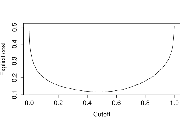
Figure 4.1: Cost Value over Cut-off of Train Dataset

Table 4.1: Confusion Matrix with Cut-off $0.49$ of Train Dataset

		Predictive
		False	True
Actual	0	5683 (TN)	899 (FN)
	1	638 (FP)	6129 (TP)

Figure 4.2: ROC Curve on Test Dataset

Table 4.2: Static Information of Selected Features of Test Dataset

Notation	Min.	1st Qu.	Median	Mean	3rd Qu.	Max.
$n$	15.00	19.00	20.00	20.62	23.00	25.00
$m$	8.00	50.00	84.00	89.86	126.00	210.00
$\frac{1}{N^{2}}$	0.00	0.00	0.00	0.00	0.00	0.00
$\bar{S}$	58.22	312.20	476.90	464.20	565.50	993.60
$c_{ij}$	0.00	2.50	5.00	5.01	7.52	10.00
$f_{ij}$	20000.00	30150.00	40260.00	40140.00	50180.00	60000.00
$\gamma_{ij}$	2024.00	5256.00	8038.00	42790.00	15940.00	78880000.00
$\bar{l}_{ij}$	0.00	0.00	0.00	0.01	0.00	0.99
$t_{i}$	-1.00	-1.00	0.00	0.15	1.00	1.00
$\bar{r}_{i}$	-1.00	-0.10	0.00	0.00	0.09	0.99
$\bar{r}_{i*}^{S}$	0.00	0.47	0.68	0.65	0.86	1.00
$\bar{r}_{i*}^{D}$	-1.00	-0.88	-0.68	-0.65	-0.46	0.00
$\bar{r}_{*i}^{S}$	0.00	0.00	0.00	0.65	1.09	16.11
$\bar{r}_{*i}^{D}$	-19.00	-0.98	0.00	-0.66	0.00	0.00
$\bar{d}_{i*}$	0.04	0.50	0.68	0.65	0.83	0.96
$\bar{d}_{i*}^{S}$	0.00	0.19	0.27	0.27	0.36	0.61
$\bar{d}_{i*}^{D}$	0.00	0.10	0.18	0.18	0.25	0.48
$\bar{d}_{*i}$	0.04	0.50	0.68	0.65	0.83	0.96
$\bar{d}_{*i}^{S}$	0.00	0.00	0.00	0.27	0.60	0.96
$\bar{d}_{*,i}^{D}$	0.00	0.00	0.00	0.19	0.35	0.96
$y_{ij}$	0.00	0.00	0.00	0.07	0.00	1.00

Furthermore, the model is validated on test data set, which is never touched before. The statistics information of test data set is summarized in Table 4.2, in which we can see the number of nodes ranges between $15$ and $25$. Therefore, the problems solved in the test data set are larger than train data and none of problems exist in both data sets. Firstly, Table 4.3 reports the confusion matrix applied test data set with cut-off point of $0.49$. According to the table, the predictive model also performs well. Secondly, receiver operating characteristic (ROC) is used to measure the performance of the predictive mode as the cut-off point is varied. This curve is created by true positive rate and false positive rate. The diagonal is called random guess line since that if we guess randomly, $FPR$ and $TPR$ are $50\%$ to $50\%$ (Figure 4.2). The ROC space is the distance between point on ROC curve and line. The best possible prediction yield the left corner point $(0,1)$ which is also named perfection classification. In this test, the area under ROC curve achieves $0.95$.

Table 4.3: Confusion Matrix with Cut-off $0.49$ of Test Dataset

		Predictive
		False	True
Actual	0	29820 (TN)	5363 (FN)
	1	221 (FP)	2246 (TP)

In summary, through rigorous validation process, it can be inferred that the logistic regression model is accurate on both train data set and test data set. The final model is displayed in Table 3.3 and the cut-off point is set as $0.49$ in the Chapter 5.

4.2 Interpretation of Logistic Regression Model

This section interprets the notations and the corresponding values in the logistic regression model in detail. Firstly, the model is in agreement with some intuitive network characteristics and quantifies the exact effect statistically. In Table 3.3, $m$ denotes the total number of arcs in the network and is statistical significant in terms of the low p-value ($0.003$) and the high significant code (‘***’ refers to the most significance). The logistic parameter of $m$ ($\beta_{m}$) equals $-5.52E-03$ with the standard error of $1.86E-03$ and the corresponding odds ratio is $0.994$, which is obtained by taking the exponential of $\beta_{m}$. This is to say, holding every predictors constant except $m$, when the network has one more arc, the response variable decreases by $0.5\%$. Intuitively, more arcs in the network results in more alternative paths exiting in the network. Therefore, the overall probability for an arc to be selected in the optimal solution is naturally negative correlated with the number of arcs. Both variable and fixed costs have a significantly effect on the response variables as showed in Table 3.3. The $1$-unit increase of variable cost and fixed cost can drop the response variable by $8.4\%$ and $0.01\%$, respectively. However, we can not directly infer that variable costs are more influential than fixed costs, since the odds ratio should be combined with the range of the predictors to evaluate the impact. As shown in Table 3.2, the range of $c_{ij}$ is $10$ and the corresponding of response variable has maximum $84\%$ increase/decrease, while the $f_{ij}$ can vary between $20,000$ and $60,000$, hence the possible corresponding probability can increase/decrease by $400\%$ at most. Consequently, fixed cost has more effect with above variety with this range.

Secondly, two hidden findings can be concluded from the model. Although fixed and variable costs are statistical significant, the ratio between them is not so important because the p-value is $0.27$ and the odds ratio of $\gamma_{ij}$ is $1.000000128$, close to $1$. In addition, total supply requirements and density are involved in our candidate predictors, but they are not statistically significant in terms of Akaike information criterion. Therefore, the accuracy of the predictive model is not affected by total supply requests and the network density.

Thirdly, an arc is whether or not used in the FCNF is notably affected by the corresponding head and tail nodes because almost all the features of nodes are statistically significant. For example, the response variable increases by $779\%$ if the type of head node changes from demand to supply. This could also be verified by the odds ratio of $\bar{r}_{i}$, which indicates that $1$-unit increase of the requests of head node leads to $162\%$ increase of response variable. Keeping the other predictors constant, if the indegree of the head node increase $1$-unit, there is $93\%$ decrease of the response variable. The other relationships can be found in Table 3.3.

Finally, an arc has positive flow in the linear relaxed FCNF has a much higher probability to be used in the original FNCF. With the notable influence of $\bar{l}_{ij}$, the response variable is $3,1730\%$ more likely to be used when the flow of arc increases from zero to full capacity. If an arc is open in the linearized FCNF, the likelihood of this arc has positive flow increases by $307\%$. This property is commonly employed to improve the branch and bound technique at either root node or branch nodes [24, 17, 34, 53]. This paper provides statistical evidence to support these works but also indicates the non-negligible difference between the optimal solutions of the linear relaxation problem and the original FCNF. In order to illustrate the problem, we build a logistic regression model on the train dataset only with one predictor ( $\bar{l}_{ij}$) and the confusion matrix is showed in Table 4.4. The total false cost of Table 4.4 is $0.21$, while the logistic regression model (Table 3.3) is only $0.11$, in which other predictors revise the misclassification of $\bar{l}_{ij}$. All these findings can be applied to analyze the networks characteristics, identify critical components of the network and provide preprocessing information to the FCNF problem.

Table 4.4: Confusion Matrix of logistic regression with only $l_{ij}$ on Train Dataset

		Predictive
		False	True
Actual	0	6187 (TN)	395 (FN)
	1	2844 (FP)	3923 (TP)

Chapter 5 Applications of Predictive Model

5.1 Important Index and Case Study

According to literature review in Section 1.2, to identify the critical components or develop components importance index (CII), a measure is required to evaluate the network performance. In this thesis, the objective value of the optimal solution in FCNF is employed to quantify the network service level. The objective value is not a single cost value, but results through solving the FCNF. The optimal solution considers many metrics that are widely used individually to evaluate the network, e.g. network flow, link capacity, delivery costs and network connectivity. Since FCNF is NP-hard and computational expensive to find the optimal solution, no existing literature uses it to measure the network performance. When the problem extends to identify critical groups of edges of different sizes over the entire network, it is a NP-complete combination problem, which is difficult to solve by itself. The predictive model provides a efficient, simple, inexpensive and practical way to compute the CII for each arc in terms of FCNF without solving any NP-complete or NP-hard problems, which extends the metrics of evaluating network performance family.

The CII is defined as the probability that an arc is selected in the optimal solution of the FCNF for the reason that, intuitively, destruction or damaging of arcs in the optimal solutions causes a rerouting of the flow from optimal path to a non-optimal path with higher costs between supply and demand nodes. The higher probability indicates the arc is more important and vice verse. To formulate the measure, let $\pi_{ij}$ denote the likelihood that arc $(i,j)\in A$ is used in the optimal solution, the value of which is directly from the predictive model developed in Section 3.3. Let $b_{ij}$ represent whether or not to remove arc $(i,j)\in A$ from the network,

$$b_{ij}=\begin{cases}0,\text{remove arc (i,j)}\\ 1,\text{otherwise}\end{cases}\forall(i,j)\in A.$$

Furthermore, let $z=z(b_{ij})$ where $z(b_{ij})$ represents the relationship between total cost of the network and removal status of arc $(i,j)\in A$,

$$z(b_{ij})=\text{min} \sum_{(i,j)\in A}(c_{ij}x_{ij}+f_{ij}y_{ij})$$

s.t. $$\sum_{(i,j)\in A}x_{ij}-\sum_{(j,i)\in A}x_{ji}=R_{i} \forall{i\in N}$$

$$0\leq x_{ij}\leq M_{ij}y_{ij} \forall{(i,j)\in A}$$

$$y_{ij}\in\{0,1\} \forall{(i,j)\in A}$$

$$y_{ij}\leq b_{ij} \forall{(i,j)\in A}$$

$$b_{ij}\in\{0,1\} \forall(i,j)\in A$$

Finally, we define the failure effect as the percentage increase of cost caused by the disruption of segments compared with the cost incurred when all arcs are present in the network ($b_{ij}=0,\forall(i,j)\in A$) represented by $z_{0}$. Let $\eta(b_{ij})$ denote the failure effect and the equation is expressed as,

$$\eta(b_{ij})=\dfrac{z(b_{ij})-z_{0}}{z_{0}}\times 100\%$$

In real-world, it is not practical to solve the large FCNF problem exactly and the value of $\eta_{ij}$ is unavailable due to the computational difficulty. According to our experiments, the solving time increase significantly when the number of nodes achieves $30$. However, the predictive model is simply linear calculation and can output the results immediately. The critical components measure approach is illustrated with a random directed network as depicted in Figure 5.1. Node 1, 7 and 9 are supply nodes and node 0, 5 and 6 are demand nodes. The arrow on the line indicates the direction and each node-pair has two directed arcs, thus we total have $28$ arc variables. The value of $z_{0}$ for this instance is $316074$.

Figure 5.1: Small Directed Network with $10$ Nodes and $28$ Arcs

Table 5.1 displays the variable cost, fixed cost, probability to be in optimal solution, failure effect for each arc comprising the network. Note, since this is a directed network, arc $(0,1)\in A$ is not same as arc $(1,0)\in A$. Based on this table, both the probability of arc $(7,6)$ and $(9,0)$ is $0.99$, and their failure effects are $10.22\%$ and $6.78\%$, respectively. Although they do not have the lowest variable cost or fixed cost, the endpoints of these two arcs are a pair of supply and demand nodes. The predictive model automatically considers all the features of this arc and give the probability that the likelihoods of these two arcs to be selected in the optimal solution are close to $1$. Some arcs with low costs, e.g. $(6,7)$, $(0,9)$, $(8,0)$, $(5,8)$ and $(8,7)$, have high CII values as well. These arcs can be contrasted with arcs with very low CII values, which means they do not contribute to any failure effects. In addition, according to the table, the directed arcs connecting same pair of nodes do not share same failure effect and probability. For example, the value of probability and failure effect of arc $(9,4)$ are much higher than arc $(4,9)$. Consequently, it is non-trivial to consider the direction of arcs in the identification of critical components. Finally, optimization approach to Zio et al. [63], Shen et al. [46] can only find the optimal critical segments in the network, but the predictive model is capable to calculate CII for each bridge. Accordingly, decision maker can combine the CII with other indices, e.g. social and economic, to select critical components.

Table 5.1: Probability and Failure Effect for Each Arc in Network

Arc$(i,j)$	$c_{ij}$	$f_{ij}$	$\pi_{ij}$	$\eta_{ij}$
(7,6)	7.20	41011.33	0.99	10.22 %
(9,0)	6.51	44846.94	0.99	6.78 %
(9,4)	5.95	22028.81	0.95	7.81 %
(1,0)	9.69	42158.06	0.95	7.81 %
(6,7)	1.93	24561.20	0.82	10.22 %
(1,2)	7.17	44364.01	0.73	0.37 %
(0,9)	3.10	28765.87	0.66	6.78 %
(8,0)	7.54	26588.18	0.49	4.54 %
(2,5)	8.90	52552.74	0.45	0.37 %
(5,8)	3.90	28365.83	0.35	7.81 %
(7,3)	1.47	43307.38	0.23	7.81 %
(8,7)	0.13	33349.63	0.17	7.81 %
(4,6)	9.09	53894.90	0.11	4.54 %
(3,7)	4.93	40543.16	0.09	0.37 %
(7,8)	5.68	49949.96	0.09	0.00 %
(0,1)	1.27	56093.72	0.04	0.00 %
(2,3)	5.90	31594.21	0.03	0.00 %
(5,2)	2.53	46060.27	0.03	0.00 %
(4,9)	1.21	48247.28	0.03	0.00 %
(8,5)	4.01	57456.67	0.02	0.00 %
(0,8)	8.61	47039.03	0.02	0.00 %
(3,2)	3.43	41127.17	0.01	0.00 %
(2,1)	5.07	50998.22	0.01	0.00 %
(6,4)	7.67	48589.75	0.01	0.00 %
(4,2)	7.62	39342.56	0.01	0.00 %
(4,3)	4.77	46389.37	0.00	0.00 %
(3,4)	6.18	48528.36	0.00	0.00 %
(2,4)	3.63	54166.87	0.00	0.00 %

In order to evaluate the quality of critical identification method, the experiment design includes tests on a variety of network densities, each which has characteristics corresponding to difficult FCNF problem instances (e.g. high fixed to variable cost ratio). The tests consists of $100$ networks with $20$ nodes, for which we can solve optimally in a reasonable time horizon. Specifically, we create a connected network with the number of arcs randomly selected between $38$ to $380$. In this experiment, we perform comparison of failure effect by blocking two arcs with highest CII and two arcs with lowest CII. The distribution of failure effect by removing top two critical arcs is displayed in Figure 5.2. Among all the $100$ instances, the blockage of the two critical arcs leads to average $9.85\%$ increase of network cost and in some cases, the failure effect achieves over $30\%$. However, the failure effects of two non-critical arcs are average to $0.21\%$ and in the $94$ instances among tests, the failure effects are $0\%$. Consequently, it is reasonable to conclude that the arcs with higher CII values can lead to more failure effects and should be protected as critical segments.

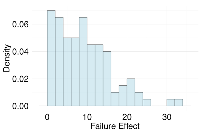
Figure 5.2: Distribution of Failure Effect by Removing Top Two Critical Arcs

5.2 Regression Based Relaxation

5.2.1 RBR Formulation

In this section, a novel approximate solution approach to the FCNF based on the predictive model is discussed, which is named regression-based relaxation (RBR). Let $p_{ij}$ denote the probability that arc $(i,j)\in A$ is open in the FCNF problem, which is calculated by the predictive model. Let $c^{{}^{\prime}}_{ij}=-\ln p_{ij}$ where $0<p_{ij}\leq 1(\forall(i,j)\in A)$ and $z^{\prime}_{\text{RBR}}$ denote the objective value of the RBR FCNF, which is defined as

$$z^{\prime}_{\text{RBR}} =\sum_{(i,j)\in A}c^{{}^{\prime}}_{ij}x_{ij}$$

$$=\sum_{(i,j)\in A}-x_{ij}\ln p_{ij}$$

$$=-\ln\prod_{(i,j)\in A}p_{ij}^{x_{ij}}$$

The RBR problem formulation is: $\min z^{\prime}_{\text{RBR}}$ subject to (2.2) – (2.4). In a simple case with single supply node $s$, single demand node $t$, and total network supply equal to 1 in a feasible problem, the RBR solution will be a most probable feasible path from $s$ to $t$. That is, if $P_{st}$ denotes a most probable feasible path from $s$ to $t$,

$$\min z^{\prime}_{\text{RBR}}=-\ln\prod_{(i,j)\in P_{st}}p_{ij}$$

and $x_{ij}=1\iff x_{ij}\in P_{st}$. In general for feasible FNCF problems with $\mathbf{x}\geq 0$, the solution to RBR identifies a set of arcs which form feasible likely paths from possibly many supply nodes to many demand nodes.

Here, the RBR problem is linear and can be solved immediately. The optimal solution of RBR is easily transformed to a feasible solution of the original FCNF. Let $x_{ij}^{*}$ denote the value of optimal flows on arc $(i,j)\in A$ in the RBR problem, and the corresponding decision variables, $y_{ij}^{*}$ , are assigned as,

$$y^{*}_{ij}=\begin{cases}1,x^{*}_{ij}>0\\ 0,\text{otherwise}\end{cases}\forall{(i,j)\in A}.$$ (5.1)

The updated solution satisfies all the constraints in the FCNF. Let the objective value of the FCNF found using RBR be denoted by $z_{RBR}$ and calculated by,

$$z_{RBR}=\sum_{(i,j)\in A}(c_{ij}x^{*}_{ij}+f_{ij}y^{*}_{ij}).$$

5.2.2 RBR Computation Results

In order to evaluate the solution quality and efficacy of the RBR approximate solution approach to the FCNF, we randomly generate 626 FCNF instances as the test bed, which includes a large variety of network sizes and all the instances have characteristics with respect to difficult FCNF (high fixed and variable cost ratio). The tests are classified into three levels by the number of nodes, 224 easy ($10-300$ nodes), 236 medium ($350-650$ nodes), and 166 hard ($700-1000$ nodes) problems. The number of arcs, $m$, is randomly selected. The percentage of supply, demand and transshipment nodes are randomly chosen with respectively approximate probabilities, $0.2$, $0.2$, and $0.6$. The probabilities are approximate because adjustments are necessary to ensure the instance is feasible. The variable costs and fixed costs follow $\text{U}(0,10)$ and $\text{U}(20000,60000)$, respectively. The total number of supplies is randomly assigned on $\text{U}(1000,2000)$.

Let $\rho_{s}$ and $\rho_{d}$ denote the percentage of supply and demand nodes, respectively. Table 5.2 reports the statistics of the network characteristics of the test bed (Min., 1st Qu., Median, Mean, 3rd Qu. and Max.). The smallest instance is composed of 10 nodes and 20 directed arcs, which is close to the problem size of train dataset, whereas the largest problem contains $1,000$ nodes and $82,010$ arcs, which is extremely lager than the network in train and test dataset. Furthermore, the first quarter of number of nodes is $250$ which is also much larger than the largest problem in train and test dataset. The average supply quantity ranges from $333$ to $1,971$. The ratio of fixed costs to variable costs averages to $8,008$. The test bed includes FCNF instances with $10\%$ to $50\%$ of nodes as supply nodes, and $8\%$ to $40\%$ as demand nodes.

The experiments employs linear programming (LP) relaxation and state-of-the-art exact technique as the benchmarks. The objective value of the FCNF found using LP relaxation is denoted by $z_{\text{LP}}$. We select state-of-the-art Gurobi software as the exact optimization technique, which is a commercial optimization (linear, integer and mixed integer programming) software. By default setting, Gurobi uses 14 different MIP heuristics, 16 cutting plane strategies, and several presolve techniques [42]. The best objective value found using Gruobi 5.6.3 is denoted as $z_{\text{GRB}}$. The experiments are performed on a Windows 7 64bit machine with Intel Xeon CPU E5-1620 and 8 GB RAM. The time limit for all three techniques is 60 seconds and the actual running time for RBR, LP and Gurobi are recoded as $t_{\text{RBR}},t_{\text{LP}}$ and $t_{\text{GRB}}$, respectively.

Table 5.2: Statistics Information of the Test Bed

Paramters	Min.	1st Qu.	Median	Mean	3rd Qu.	Max.
$n$	10	250	400	446.7	700	1000
$m$	20	9497	26270	29520	46480	82010
$\rho$	0.03	0.24	0.58	0.55	0.89	1.00
$\bar{S}$	333	858.2	947	968.4	1039	1971
$\gamma$	7110	7986	8000	8008	8010	9809
$\rho_{s}$	0.1000	0.3000	0.3178	0.3173	0.3329	0.5000
$\rho_{d}$	0.0800	0.1887	0.2000	0.2033	0.2161	0.4000

In this section, we report the analysis of solution quality and efficiency of RBR, LP and Grurobi. Let $z_{\text{gap}}^{x}$ denote the percentage gap between $z_{\text{RBR}}$ and $z_{x}$,

$$z_{\text{gap}}^{x}=\dfrac{z_{\text{RBR}}-z_{x}}{|z_{x}|}\times 100\%.$$ (5.2)

where $z_{x}$ is one of $z_{\text{LP}}$ or $z_{\text{GRB}}$. Let $t_{\text{diff}}^{x}$ denote how many times RBR is faster/slower than $x\in\{\text{LP},\text{GRB}\}$,

$$t_{\text{diff}}^{x}=\dfrac{t_{x}}{t_{\text{RBR}}},$$ (5.3)

here, if $t_{\text{diff}}^{\text{LP}}$ equals to $2$, then solving the RBR problem is twice faster than solving the LP problem; reversely, if $t_{\text{diff}}^{\text{LP}}$ equals to $0.5$, then $t_{\text{RBR}}$ is twice longer than $t_{\text{LP}}$.

The performance is measured with respect to $z_{\text{gap}}^{x}$ and $t_{\text{diff}}^{x}$ together. Based on the formulation (5.2), if RBR outperforms LP (Gurobi) in terms of objective value, the value of $z_{\text{gap}}^{LP}$ ($z_{\text{gap}}^{GRB}$) is negative; if RBR outperforms LP (Gurobi) with respect to CPU time, the value of $t_{\text{diff}}^{LP}$ ($t_{\text{diff}}^{GRB}$) is larger than $1$. Let binary variable $\theta_{x}$ denote whether RBR outperforms $x\in\{\text{LP},\text{GRB}\}$,

$$\theta_{x}=[z_{\text{gap}}^{x}<0][t_{\text{diff}}^{x}>1]$$

where, $[X]$ returns $1$ if $X$ is true; otherwise, returns $0$. In this investigation, we claim RBR outperforms LP (Gurobi) only when $\theta_{\text{LP}}=1$ ($\theta_{\text{GRB}}=1$), respectively. Table 5.3 reports the experimental results by techniques.

Table 5.3: Objective Gap and Time Difference Statistics

		Levels
		Easy	Medium	Hard	Overall
RBRvsLP	$\theta_{\text{LP}}=1(\%)$	91.96	100	100	97.12
	min $z_{\text{gap}}^{\text{LP}}(\%)$	-43.39	-45.05	-46.94	-46.94
	mean $z_{\text{gap}}^{\text{LP}}(\%)$	-25.23	-35.57	-36.18	-32.03
	max $z_{\text{gap}}^{\text{LP}}(\%)$	0.00	-11.96	-7.31	0.00
	min $t_{\text{diff}}^{\text{LP}}$	1.26	3.17	2.93	1.26
	mean $t_{\text{diff}}^{\text{LP}}$	24.65	41.48	26.55	31.5
	max $t_{\text{diff}}^{\text{LP}}$	147	186.2	116.9	186.2
RBRvsGRB	$\theta_{\text{GRB}}=1(\%)$	5.28	46.41	98.05	51.69
	min $z_{\text{gap}}^{\text{GRB}}(\%)$	-20.60	-41.17	-44.93	-44.93
	mean $z_{\text{gap}}^{\text{GRB}}(\%)$	14.29	-1.25	-29.84	-6.16
	max $z_{\text{gap}}^{\text{GRB}}(\%)$	51.20	32.68	14.62	51.20
	min $t_{\text{diff}}^{\text{GRB}}$	3.31	87.41	11.28	3.31
	mean $t_{\text{diff}}^{\text{GRB}}$	5756	591	177	2052
	max $t_{\text{diff}}^{\text{GRB}}$	82430	5752	2791	82430

Overall, RBR outperforms LP in $97.12\%$ of the test bed and is never outperformed by LP (the maximum value of $z_{\text{gap}}^{\text{LP}}$ is $0.00\%$). Figure 5.3 shows the distribution of objective gap between RBR and LP by difficult levels. RBR finds objective values average $32.03\%$ lower than LP relaxation solution approach. The percentage of FCNF instances in which RBR outperforms LP in both solution quality and efficiency achieves $100\%$ for the medium and hard problems. For some specified instances, RBR performs quite well and the highest improvement of RBR to LP achieves $46.94\%$. In addition, running time of solving a RBR problem is overall $31.5$ times faster than solving a LP relaxation problem. Based on the minimum value of $t_{\text{diff}}^{\text{LP}}$ ($1.26$), there does not exist a problem instance in which RBR uses longer time than LP. Figure 5.4 plots the running time as a function of the number of variables, from which it is observed that the running time of RBR is not affected apparently by the size of the problem instances (average $t_{\text{RBR}}=0.33$ seconds), albeit the running time of LP appears exponential relationship with the number of variables (average $t_{\text{LP}}=12.75$ seconds). Specifically, LP performs equally with RBR only when the number of nodes is less than $10$. Therefore, RBR is guaranteed to find a better solution in a shorter time period than LP regardless of the scale and complexity of FNCF problem.

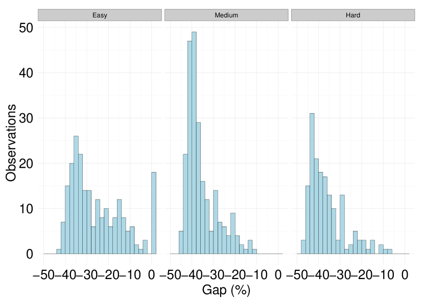
Figure 5.3: Distribution of Gap between $z_{RBR}$ and $z_{\text{LP}}$ by Level

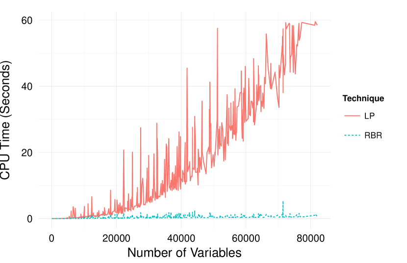
Figure 5.4: CPU Time of RBR and LP over Number of Variables

State-of-the-art exact solver outperforms RBR with respect to solution quality in $95\%$ of the test instances, but solving RBR problem is overall $5,756$ times faster than GRB with 60 seconds limit. In detail, GRB achieves the time limit ($60$ seconds) when the number of variables is $220$, in which RBR only runs around $0.001$ seconds. The solution produced by RBR begins showing comparable to Gurobi when the difficult level is medium. Figure 5.5 shows the gap distribution between $z_{RBR}$ and $z_{GRB}$ by difficult level. For hard FCNF problems, RBR outperforms Gurobi in $98\%$ of the hard instances and is only outperformed by Gurobi in $5$ over $248$ hard cases. The average improvement for hard instances is around $30\%$ with much less running time. Since the running time of Gurobi is always extended to $60$ seconds while average RBR running time is only $0.33$ seconds, the investment in involving RBR as a pre-prosessing technique to the FCNF is efficient. Specifically, RBR could could find a better upper bound in the solving process and then reduce total running time of optimization solver.

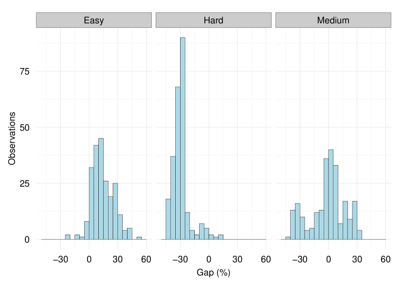
Figure 5.5: Distribution of Gap between $z_{RBR}$ and $z_{\text{GRB}}$ by Level

Chapter 6 Conclusion

The fixed charge network flow problem has many real-world applications and can be transformed to various problem types. Because it is a classically NP-hard problem, many approximate algorithms have been developed to find a near-optimal solution in a reasonable time period. This research provides a novel and original framework to analyze the optimal flow of the FCNF. In this work, we address three questions in terms of the analysis, prediction and application.

Firstly, by analyzing the possible features that may affect the optimal flow, we follow three levels from the entire network to an arc and to a single node to ensure we extract all the useful features. There are $33$ independent features and only $26$ of them are employed as predictors for the final predictive model with respect to Akaike information criterion. The validation process includes most common diagnostic techniques, e.g. confusion matrix, k-fold cross validation, ROC curve. The results indicate that the predictive ability is highly accurate on both train dataset and test dataset. According to the model, we can conclude that: (1) as the increase of network size, the average probability for each arc decreases; (2) the characteristics of arcs (e.g. variable and fixed costs) and nodes (e.g. node type and degree) have a statistical significant effect on the likelihood; (3) the logistic regression model is in agreement with that the linear relaxation and original problem share a significant proportion of optimal arcs. However, our study also finds that the linear relaxed FCNF loses considerable number of optimal arcs in the original problems. The rest predictors play an important role on improving the predictive capability. It is observed that the types of nodes of the arc and endpoints adjacent to the nodes provide a vital contribution in reducing the predictive errors.

Secondly, this predictive model can be used directly to identify critical arcs in the network. The component importance index (CII) is defined as the likelihood that the arc is selected in the optimal solution and the network performance is evaluated by the objective value of the FCNF. In our rigorous tests, the failure effects cased by high-CII arcs are statically significant than cased by low-CII arcs. The FNCF has never been used to measure the network performance due to the computational difficulty, not to mention quantifying the failure effect for each arc. The values of CII in our experiments are consistent with the failure effects and rank all the arcs, which supports the decision make on critical components identification or priorization.

Finally, the other application of the predictive mode is presented in the work, which we name regression-based relaxation (RBR). The RBR solution approach replaces the objective function with the natural logarithm of the product of probabilities calculated by predictive model. Then, the optimal solution of RBR problem is the most probable feasible path of the original FCNF problem. The solution quality of RBR is compared with linear programming relaxation solution approach, and state-of-the-art optimization software. The rigorous experiments show that RBR outperforms LP in $97.12\%$ of the test bed and produced objective values average $32.03\%$ lower than LP on average. Overall, solving a RBR problem is $31.5\%$ times faster then solving a LP problem. The empirical results indicates RBR stably outperforms Gurobi in the large-scale and high-complexity FNCF problems.

In summary, it is the first time to combine statistical learning technique and network flow problem. There are several vital network characteristics affecting the optimal flow regardless of the density and total requirements of the problem. The predictive model provides a novel approach to analyze and predict the optimal flow, which can be used independently on the identification of the critical components or approximate solution approach to the FCNF.

The regression-based relaxation is one of possible applications and shows great advantage over the linear programming and standard exact technique. In the future work we will explore more applications that most benefit from this predictive model.

Chapter 7 Future Research

Solution approach to discrete optimization has been popular for many years, but still a evolving research area. This research is the first to apply machine learning algorithms to study the optimal flows of the FCNF instead of transitional approach. We exploited the special structures of the FCNF problem and presented two possible applications. As part of our research, we identify the following important research topics that we plan to explore.

1. Network Science. Currently, many research topics have transfered from single object to a group of homogeneous or inhomogeneous objects, e.g., transportation network, social network and community networks, etc. Network science, as a maturing field, offers a unique perspective to tackle complex problems, impenetrable to linear-proportional thinking. The framework proposed in this work is for a specified optimization problem, but the concept or procedure can be applied to all types of networks with modification of features. In the future work, more types of network problems will be explored by this procedure and reversely, these networks can be employed to validate the methodology.

2. Solution Approach to difficult optimization problem. Due to the success of regression-based relaxation, we plan to develop strategy combing the RBR and Branch-and-bound technique to provide a high efficiency exact solution approach to the FCNF problem. Furthermore, many difficult optimization problems has their own characteristics, such like Knapsack problem, traveling salesman problem, and job shop scheduling, etc, thus, we can study the parameters, decision variables and constraints of these problems and develop predictive model based on the known optimal solution.

3. Scala Machine Learning. As the datasets growing exponentially, many machine learning techniques are not practical to apply because of the limitation of computational power. Scala machine learning is a relative new area in artificial intelligent area. According to the experimental results in this work, the predictive model can be trained on a small data set of easy-solve instances, and keep its highly accuracy for larger and more complex problems. This conclusion is same as Scala Machine Learning and we plan to explore methods to apply machine learning algorithms to big data more reliably and efficiently.

References

- Akaike [1974] H. Akaike. A new look at the statistical model identification. Automatic Control, IEEE Transactions on, 19(6):716–723, 1974.
- Armacost and Ware [2002] C. Armacost, A. Barnhart and K. Ware. Composite variable formulations for express shipment service network design. Transportation science, 36(1):1–20, 2002.
- Balinski [1961] M. Balinski. Fixed-cost transportation problems. Naval Research Logistics Quarterly, 8(1):41–54, 1961.
- Barker et al. [2013] K. Barker, J. Ramirez-Marquez, and C. Rocco. Resilience-based network component importance measures. Reliability Engineering & System Safety, 117:89–97, 2013.
- Barr et al. [1981] R. Barr, F. Glover, and D. Klingman. A new optimization method for large scale fixed charge transportation problems. Operations Research, 29(3):448–463, 1981.
- Bell [2000] M.G. Bell. A game theory approach to measuring the performance reliability of transport networks. Transportation Research Part B: Methodological, 34(6):533–545, 2000.
- Bier et al. [2007] V. M. Bier, E. R. Gratz, N.J. Haphuriwat, W. Magua, and K.R. Wierzbicki. Methodology for identifying near-optimal interdiction strategies for a power transmission system. Reliability Engineering & System Safety, 92(9):1155–1161, 2007.
- Birchmeier [2007] J. Birchmeier. Systematic assesment of the degree of criticality of infrastructures. In Proceedings of ESREL, pages 859–64, 2007.
- Bixby et al. [2000] E. Bixby, M. Fenelon, Z. Gu, E. Rothberg, and R. Wunderling. MIP: Theory and practice closing the gap. In System modelling and optimization, pages 19–49. Springer, 2000.
- Bompard et al. [2009] E. Bompard, R. Napoli, and F. Xue. Analysis of structural vulnerabilities in power transmission grids. International Journal of Critical Infrastructure Protection, 2(1):5–12, 2009.
- Cabot and Erenguc [1984] A. Cabot and S. Erenguc. Some branch-and-bound procedures for fixed-cost transportation problems. Naval Research Logistics Quarterly, 31(1):145–154, 1984.
- Camdeviren et al. [2007] H. Camdeviren, A. Yazici, Z. Akkus, R. Bugdayci, and M. Sungur. Comparison of logistic regression model and classification tree: An application to postpartum depression data. Expert Systems with Applications, 32(4):987–994, 2007.
- Cohen et al. [2000] R. Cohen, K. Erez, D. Ben-Avraham, and S. Havlin. Resilience of the internet to random breakdowns. Physical review letters, 85(21):4626, 2000.
- Costa [2005] A. Costa. A survey on benders decomposition applied to fixed-charge network design problems. Computers & Operations Research, 32(6):1429–1450, 2005.
- Crucitti et al. [2004] P. Crucitti, V. Latora, and M. Marchiori. Model for cascading failures in complex networks. Physical Review E, 69(4):045104, 2004.
- Crucitti et al. [2005] P. Crucitti, V. Latora, and M. Marchiori. Locating critical lines in high-voltage electrical power grids. Fluctuation and Noise Letters, 5(02):L201–L208, 2005.
- Danna et al. [2005] E. Danna, E. Rothberg, and C. Le Pape. Exploring relaxation induced neighborhoods to improve mip solutions. Mathematical Programming, 102(1):71–90, 2005.
- Demšar et al. [2008] U. Demšar, O. Špatenková, and K. Virrantaus. Identifying critical locations in a spatial network with graph theory. Transactions in GIS, 12(1):61–82, 2008.
- Dheenadayalu et al. [2004] Y. Dheenadayalu, B. Wolshon, and C. Wilmot. Analysis of link capacity estimation methods for urban planning models. Journal of transportation engineering, 130(5):568–575, 2004.
- Dobson et al. [2007] I. Dobson, B.A. Carreras, V.E Lynch, and D.E. Newman. Complex systems analysis of series of blackouts: Cascading failure, critical points, and self-organization. Chaos: An Interdisciplinary Journal of Nonlinear Science, 17(2):026103, 2007.
- Driebeek [1966] N. Driebeek. An algorithm for the solution of mixed integer programming problems. Management Science, 12(7):576–587, 1966.
- El-Sherbiny and Alhamali [2013] M. El-Sherbiny and R. Alhamali. A hybrid particle swarm algorithm with artificial immune learning for solving the fixed charge transportation problem. Computers & Industrial Engineering, 64(2):610–620, 2013.
- Eusgeld et al. [2009] I. Eusgeld, W. Kröger, G. Sansavini, M. Schläpfer, and E. Zio. The role of network theory and object-oriented modeling within a framework for the vulnerability analysis of critical infrastructures. Reliability Engineering & System Safety, 94(5):954–963, 2009.
- Fischetti and Lodi [2003] M. Fischetti and A. Lodi. Local branching. Mathematical programming, 98(1-3):23–47, 2003.
- Fügenschuh and Martin [2005] A. Fügenschuh and A. Martin. Computational integer programming and cutting planes. Handbooks in Operations Research and Management Science, 12:69–121, 2005.
- Garey and David [1979] M. Garey and S. David. Computers and Intractability: A Guide to the Theory of NP-Completeness. W. H. Freeman, New York, NY, 1979.
- Ghamlouche et al. [2003] I. Ghamlouche, T. Crainic, and M. Gendreau. Cycle-based neighbourhoods for fixed-charge capacitated multicommodity network design. Operations research, 51(4):655–667, 2003.
- Hewitt et al. [2010] M. Hewitt, G. Nemhauser, and M. Savelsbergh. Combining exact and heuristic approaches for the capacitated fixed-charge network flow problem. INFORMS Journal on Computing, 22(2):314–325, 2010.
- Hirsch and Dantzig [1954] W. Hirsch and G. Dantzig. The fixed charge problem. Technical report, DTIC Document, 1954.
- Jarvis et al. [1978] J. Jarvis, R. Rardin, V. Unger, R. Moore, and C. Schimpeler. Optimal design of regional wastewater systems: A fixed-charge network flow model. Operations Research, 26(4):538–550, 1978.
- Kennington and Unger [1976] J. Kennington and E. Unger. A new branch-and-bound algorithm for the fixed-charge transportation problem. Management Science, 22(10):1116–1126, 1976.
- Kim and Pardalos [1999] D. Kim and P. Pardalos. A solution approach to the fixed charge network flow problem using a dynamic slope scaling procedure. Operations Research Letters, 24:195–203, 1999.
- Lederer and Nambimadom [1998] P. Lederer and R. Nambimadom. Airline network design. Operations Research, 46(6):785–804, 1998.
- Lodi [2010] A. Lodi. Mixed integer programming computation. In 50 Years of Integer Programming 1958-2008, pages 619–645. Springer, 2010.
- Mahajan [2010] A. Mahajan. Presolving mixed–integer linear programs. Wiley Encyclopedia of Operations Research and Management Science, 2010.
- McLachlan et al. [2005] G. McLachlan, K. Do, and C. Ambroise. Analyzing microarray gene expression data, volume 422. John Wiley & Sons, 2005.
- Molla-Alizadeh-Zavardehi et al. [2011] S. Molla-Alizadeh-Zavardehi, M. Hajiaghaei-Keshteli, and R. Tavakkoli-Moghaddam. Solving a capacitated fixed-charge transportation problem by artificial immune and genetic algorithms with a prüfer number representation. Expert Systems with Applications, 38(8):10462–10474, 2011.
- Monteiro et al. [2011] M. Monteiro, D. Fontes, and F. Fontes. An ant colony optimization algorithm to solve the minimum cost network flow problem with concave cost functions. In GECCO, pages 139–146, 2011.
- Nemhauser and Wolsey [1988] G. Nemhauser and L. Wolsey. Integer and combinatorial optimization, volume 18. Wiley New York, 1988.
- Nicholson and Zhang [2016] Charles D Nicholson and Weili Zhang. Optimal network flow: A predictive analytics perspective on the fixed-charge network flow problem. Computers & Industrial Engineering, 99:260–268, 2016.
- Nozick [2001] L. Nozick. The fixed charge facility location problem with coverage restrictions. Transportation Research Part E: Logistics and Transportation Review, 37(4):281–296, 2001.
- Optimization [2012] Gurobi Optimization. Inc.. gurobi optimizer reference manual, version 5.0, 2012.
- Ortega and Wolsey [2003] F. Ortega and L. Wolsey. A branch-and-cut algorithm for the single-commodity, uncapacitated, fixed-charge network flow problem. Networks, 41(3):143–158, 2003.
- Palekar et al. [1990] U. Palekar, M. Karwan, and S. Zionts. A branch-and-bound method for the fixed charge transportation problem. Management Science, 36(9):1092–1105, 1990.
- Scott et al. [2006] D.M. Scott, D.C. Novak, L. Aultman-Hall, and F. Guo. Network robustness index: a new method for identifying critical links and evaluating the performance of transportation networks. Journal of Transport Geography, 14(3):215–227, 2006.
- Shen et al. [2012] S. Shen, J. Smith, and R. Goli. Exact interdiction models and algorithms for disconnecting networks via node deletions. Discrete Optimization, 9(3):172–188, 2012.
- Smith et al. [2003] B.L. Smith, L. Qin, and R. Venkatanarayana. Characterization of freeway capacity reduction resulting from traffic accidents. Journal of Transportation Engineering, 129(4):362–368, 2003.
- Stehman [1997] S.V. Stehman. Selecting and interpreting measures of thematic classification accuracy. Remote sensing of Environment, 62(1):77–89, 1997.
- Steinberg and Napier. [1980] E. Steinberg and H. Napier. Optimal multi-level lot sizing for requirements planning systems. Management Science, 26(12):1258–1271, 1980.
- Sun et al. [1998] M. Sun, J. Aronson, P. McKeown, and D. Drinka. A tabu search heuristic procedure for the fixed charge transportation problem. European Journal of Operational Research, 106(2):441–456, 1998.
- Venables and Ripley [2002] W. Venables and B. Ripley. Modern applied statistics with S. Springer, 2002.
- Wolsey [1998] L. Wolsey. Integer programming, volume 42. Wiley New York, 1998.
- Zhang and Nicholson [2014] W. Zhang and C. Nicholson. Objective scaling ensemble approach for integer linear programming. Manuscript Submitted for Publication, 2014.
- ZHANG and ZHAO [2010] Wei-li ZHANG and Lin-du ZHAO. Lattice gas model for simulating pedestrian evacuation in the dormitory fire [j]. Journal of Safety and Environment, 1:045, 2010.
- Zhang and Nicholson [2016a] Weili Zhang and Charles Nicholson. A multi-objective optimization model for retrofit strategies to mitigate direct economic loss and population dislocation. Sustainable and Resilient Infrastructure, 1(3-4):123–136, 2016a.
- Zhang and Nicholson [2016b] Weili Zhang and Charles D Nicholson. Prediction-based relaxation solution approach for the fixed charge network flow problem. Computers & Industrial Engineering, 99:106–111, 2016b.
- Zhang and Wang [2016] Weili Zhang and Naiyu Wang. Resilience-based risk mitigation for road networks. Structural Safety, 62:57–65, 2016.
- Zhang and Wang [2017] Weili Zhang and Naiyu Wang. Bridge network maintenance prioritization under budget constraint. Structural safety, 67:96–104, 2017.
- Zhang and Yao [2010] Weili Zhang and Zhengyu Yao. A reformed lattice gas model and its application in the simulation of evacuation in hospital fire. In Industrial Engineering and Engineering Management (IEEM), 2010 IEEE International Conference on, pages 1543–1547. IEEE, 2010.
- Zhang et al. [2017] Weili Zhang, Naiyu Wang, and Charles Nicholson. Resilience-based post-disaster recovery strategies for road-bridge networks. Structure and Infrastructure Engineering, 13(11):1404–1413, 2017.
- Zhang et al. [2018] Weili Zhang, Peihui Lin, Naiyu Wang, Charles Nicholson, and Xianwu Xue. Probabilistic prediction of postdisaster functionality loss of community building portfolios considering utility disruptions. Journal of Structural Engineering, 144(4):04018015, 2018.
- Zheng et al. [2007] J. Zheng, Z. Gao, and X. Zhao. Clustering and congestion effects on cascading failures of scale-free networks. EPL (Europhysics Letters), 79(5):58002, 2007.
- Zio et al. [2012] E. Zio, L.R. Golea, et al. Identifying groups of critical edges in a realistic electrical network by multi-objective genetic algorithms. Reliability Engineering & System Safety, 99:172–177, 2012.