Response Time Bounds for Typed DAG Parallel Tasks on Heterogeneous Multi-cores

Abstract

Heterogenerous multi-cores utilize the strength of different architectures for executing particular types of workload, and usually offer higher performance and energy efficiency. In this paper, we study the worst-case response time (WCRT) analysis of typed scheduling of parallel DAG tasks on heterogeneous multi-cores, where the workload of each vertex in the DAG is only allowed to execute on a particular type of cores. The only known WCRT bound for this problem is grossly pessimistic and suffers the non-self-sustainability problem. In this paper, we propose two new WCRT bounds. The first new bound has the same time complexity as the existing bound, but is more precise and solves its non-self-sustainability problem. The second new bound explores more detailed task graph structure information to greatly improve the precision, but is computationally more expensive. We prove that the problem of computing the second bound is strongly NP-hard if the number of types in the system is a variable, and develop an efficient algorithm which has polynomial time complexity if the number of types is a constant. Experiments with randomly generated workload show that our proposed new methods are significantly more precise than the existing bound while having good scalability.

1 Introduction

Multi-cores are more and more widely used in real-time systems, to meet rapidly increasing requirements in performance and energy efficiency. To fully utilize the computation capacity of multi-cores, software should be properly parallelized. A representation that can model a wide range of parallel software is the DAG (directed acyclic graph) task model, where each vertex represents a piece of sequential workload and each edge represents the precedence relation between two vertices. Real-time scheduling and analysis of DAG parallel task models have raised many new challenges over traditional real-time scheduling theory with sequential tasks, and have become an increasingly hot research topic in recent years.

Many modern multi-cores adopt heterogeneous architectures. Examples include Zynq$-$7000 [37] and OMAP1/OMAP2 [33] that integrate CPU and DSP on the same chip, and the Tegra processors [36] that integrate CPU and GPU on the same chip. Heterogenerous multi-cores utilize specialized processing capabilities to handle particular computational tasks, which usually offer higher performance and energy efficiency. For example, [38] showed that a heterogeneous-ISA chip multiprocessor can outperform the best same-ISA homogeneous architecture by as much as $21\%$ with $23\%$ energy savings and a reduction of $32\%$ in energy delay product.

In this paper, we consider real-time scheduling of typed DAG tasks on heterogeneous multi-cores, where each vertex is explicitly bound to execute on a particular type of cores. Binding code segments of the program to a certain type of cores is common practice in software development on heterogeneous multi-cores and is supported by mainstream parallel programming frameworks and operating systems. For example, in OpenMP [34] one can use the proc$\_$bind clause to specify the mapping of threads to certain processing cores. In OpenCL[35], one can use the clCreateCommandQueue function to create a command queue to certain devices. In CUDA [10], one can use the cudaSetDevice function to set the following executions to the target device.

The target of this paper is to bound the worst-case response time (WCRT) for typed DAG tasks.

To the best of our knowledge, the only known WCRT bound for the considered problem model was presented in an early work [18] (called OLD-B), which is not only grossly pessimistic, but also suffers the non-self-sustainability problem. In this paper we develop two new response time bounds to address these problems:

• NEW-B-1, which dominates OLD-B in analysis precision with the same time complexity and solves its non-self-sustainability problem.

• NEW-B-2, which significantly improves the analysis precision by exploring more detailed task graph stucture information. NEW-B-2 is more precise, but also more difficult to compute.

  • We prove the problem of computing NEW-B-2 to be strongly NP-hard if the number of types is a variable.

  • We develop an efficient algorithm to compute NEW-B-2 with polynomial time complexity if the number of types is a constant.

Experiments with randomly generated parallel tasks show that the new WCRT bounds proposed in this paper can greatly improve the analysis precision. This paper focuses on analysis of a single typed DAG task, but our results are also meaningful to general system setting with multiple recurrent typed DAG tasks. On one hand, the results of this paper are directly applicable to multiple tasks under scheduling algorithms where a subset of cores are assigned to each individual parallel task (e.g., federated scheduling [29, 3, 5, 6, 30]). On the other hand, the analysis of intra-task interference addressed in this paper is a necessary step towards the analysis for scheduling algorithms where different tasks interfere with each other (e.g., global scheduling [8, 2, 32]).

2 Preliminary

2.1 Task Model

We consider a typed DAG task $G=(V,E,\gamma,c)$ to be executed on a heterogeneous multi-core platform with different types of cores. $S$ is the set of core types (or types for short), and for each $s\in S$ there are $M_{s}$ cores of this type ($M_{s}\geq 1$). $V$ and $E$ are the set of vertices and edges in $G$. Each vertex $v\in V$ represens a piece of code segment to be sequentially executed. Each edge $(u,v)\in E$ represents the precedence relation between vertices $u$ and $v$. The type function $\gamma:V\times S$ defines the type of each vertex, i.e., $\gamma(v)=s$, where $s\in S$, represents vertex $v$ must be executed on cores of type $s$. The weight function $c:V\times\mathbb{R}_{0}^{+}$ defines the worst-case execution time (WCET) of each vertex, i.e., $v$ executes for at most $c(v)$ time units (on cores of type $\gamma(v)$).

If there is an edge $(u,v)\in E$, $u$ is a predecessor of $v$, and $v$ is a successor of $u$. If there is a path in $G$ from $u$ to $v$, $u$ is an ancestor of $v$ and $v$ is a descendant of $u$. We use $\textsf{{pre}}(u)$, $\textsf{{suc}}(u)$, $\textsf{{ans}}(u)$ and $\textsf{{des}}(u)$ to denote the set of predecessors, successors, ancestors and descendants of $u$, respectively. Without loss of generality, we assume $G$ has a unique source vertex $v_{src}$ (which has no predecessor) and a unique sink vertex $v_{snk}$ (which has no successor). We use $\pi\in G$ to denote $\pi$ is a path in $G$. A path $\pi=\{\tau_{1},\cdots,\tau_{k}\}$ is a complete path iff its first vertex $\tau_{1}$ is the source vertex of $G$ and last vertex $\tau_{k}$ is the sink vertex. We use $vol(G)$ to denote the total WCET of $G$ and $vol_{s}(G)$ the total WCET of vertices of type $s$:

$$vol(G)=\sum_{u\in V}c(u),~{}~{}vol_{s}(G)=\sum_{u\in V\wedge\gamma(u)=s}c(u).$$

The length of a path $\pi$ is denoted by $len(\pi)$ and $len(G)$ represents the length of the longest path in $G$:

$$len(\pi)=\sum_{u\in\pi}c(u),~{}~{}len(G)=\max_{\pi\in G}\{len(\pi)\}.$$

      Example 2.1.

Figure 1 illustrates a typed DAG task with two types of vertices (type $1$ marked by yellow and type $2$ marked by red). The WCET of vertex is annotated by the number next to the vertex. And we can compute that $vol(G)=45$, $vol_{1}(G)=11$ and $vol_{2}(G)=34$. For a path $\pi=\{v_{0},v_{1},v_{7},v_{11},v_{12}\}$, the length is $len(\pi)=19$.

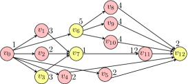
Figure 1: A typed DAG task $\tau$ with two types.

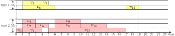
(a) An execution sequence where each vertex executes for its WCET.

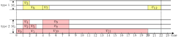
(b) An execution sequence where some vertices executes shorter than their WCET.

Figure 2: Two possible execution sequences the task in Figure1 executed on a platform with $M_{1}=2$ and $M_{2}=3$.

2.2 Runtime Behavior

A vertex is eligible for execution when all of its predecessors have finished. Without loss of generality, we assume the source vertex of $G$ is eligible for execution at time $0$. The typed DAG task $G$ is scheduled on the heterogeneous multi-core platform by a work-conserving scheduling algorithm:

      Definition 2.1.

Under a work-conserving scheduling algorithm, an eligible vertex of type $s$ must be executed if there are available cores of type $s$.

We do not put any other constraints to scheduling algorithms except the work-conserving constraint. There are many possible instances of work-conserving scheduling algorithms, e.g., the list scheduling [13] algorithm. The results of this paper are applicable to any work-conserving scheduling algorithm.

Execution Sequence. At runtime, the vertices of $G$ execute at certain time according to the scheduling algorithm. We call a trace describing which vertex executes at which time points an execution sequence of $G$. Given a scheduling algorithm, $G$ may generate different execution sequences. This is because, (1) the scheduling algorithm may have nondeterminism (the scheduler may behave differently in the same situation) and (2) each vertex may execute for shorter than its WCET. For example, Figure 2(a) shows an execution sequence where each vertex executes for its WCET, while Figure 2(b) shows another execution sequence where some vertices execute for shorter than their WCET but lead to a larger response time. In an execution sequence $\varepsilon$, we use $f_{\varepsilon}(v)$ to denote the finish time of vertex $v$. For simplicity, we omit the subscript and only use $f(v)$ to denote $v$’s finish time when the execution sequence is clear from the context.

Response Time. The response time of $G$ in an execution sequence is the finish time of the sink vertex, and the WCRT of $G$, denoted by $R(G)$, is the maximum among the response times of all possible execution sequences. The target of this paper is to derive safe upper bounds for the WCRT of $G$. Note that the WCRT of $G$ is not necessarily achieved by the execution sequence in which each vertex executes for its WCET (even if there is only one type in the system) [13, 14]. Therefore, one can not obtain the WCRT of $G$ by simply simulating the execution of $G$ using the WCET, but has to (explicitly or implicitly) analyze all the possible execution sequences of $G$.

2.3 Existing WCRT Bound

To our best knowledge, the only known WCRT upper bound for the considered model was developed in an early work [18]:

      Theorem 2.1 (OLD-B).

The WCRT of $G$ is bounded by:

$$R(G)\leq\left(1-\frac{1}{\displaystyle\max_{s\in S}\{M_{s}\}}\right)\times len(G)+\sum_{s\in S}\frac{vol_{s}(G)}{M_{s}}.$$ (1)

This bound can be computed in $O(|V|+|E|)$ time [11]. Although OLD-B was originally derived for the list scheduling algorithm [13], it applies to all work-conserving scheduling algorithms. When there is only one type, it degrades to the classical response time bound for untyped DAG tasks [14]:

$$R(G)\leq len(G)+\frac{vol(G)-len(G)}{M}.$$

3 The First New WCRT Bound

OLD-B is not only pessimistic but also suffers the problem of being non-self-sustainable with respect to processing capacity. More specifically, the value of the WCRT bound in (1) may increase when the number of cores (of some type) increases, as witnessed by the following example.

      Example 3.1.

For the task $G$ in Figure 1, we can calculate its $vol_{1}(G)=11$, $vol_{2}(G)=34$ and $len(G)=19$. Suppose $M_{1}=2$ and $M_{2}=3$, we obtain a WCRT bound by OLD-B as $29.5$. However, if we increase $M_{1}$ to $20$, the bound is increased to $29.9\dot{3}$.

Note that the actual WCRT of $G$ will not increase when more cores are used. The phenomenon shown above is merely the problem of the bound OLD-B itself rather than the system behavior. As pointed out in [1], the self-sustainability property is important in incremental and interactive design process, which is typically used in the design of real-time systems and in the evolutionary development of fielded systems.

In this section we will develop a new WCRT bound, which is not only more precise than OLD-B (with the same time complexity), but also self-sustainable. We start with introducing some useful concepts.

      Definition 3.1.

The scaled graph $\hat{G}=(V,E,\hat{c},\gamma)$ of $G=(V,E,c,\gamma)$ has the same topology ($V$ and $E$) and type function $\gamma$ as $G$, but a different weight function $\hat{c}$:

$$\forall v\in V:\hat{c}(v)=c(v)\times(1-1/M_{\gamma(v)}).$$

      Definition 3.2.

A critical path $\pi=\{\tau_{1},\cdots,\tau_{k}\}$ of an execution sequence of $G$ is a complete path of $G$ satisfying the following condition:

$$\forall\tau_{i}\in\pi\setminus\{\tau_{1}\}:f(\tau_{i-1})=\max_{u\in\textsf{{pre}}(\tau_{i})}\{f(u)\},$$

where $f(v)$ is the finish time of $v$ in this execution sequence.

For example, a complete path $\pi=\{v_{0},v_{1},v_{7},v_{11},v_{12}\}$ is the critical path for the execution sequence shown in Figure 2(a), while a complete path $\pi^{\prime}=\{v_{0},v_{2},v_{7},v_{11},v_{12}\}$ is not a critical path of this execution sequence since the $v_{2}$’s finish time is not the latest among all the predecessors of $v_{7}$.

A task $G$ may generate (infinitely) many different execution sequences at runtime, and it is in general unknown which complete path in $G$ is the critical path that leads to the WCRT. In the following, we assume an arbitrary complete path $\pi=\{\tau_{1},\cdots,\tau_{k}\}$ to be a critical path, and derive upper bounds for the response time of this particular critical path. Then by getting the maximum bound among all possible paths in $G$, we can safely bound the WCRT of $G$.

We divide $[0,f(\tau_{k}))$ into $k$ segments $[0,f(\tau_{1}))$, $[f(\tau_{1}),f(\tau_{2}))$, $\cdots$, $[f(\tau_{k-1}),f(\tau_{k}))$. For each $1<i\leq k$, we define

$$I_{i}=f(\tau_{i})-f(\tau_{i-1}),$$

and let $I_{1}=f(\tau_{1})$. We define

• $x_{i}$: the accumulative length of time intervals in $I_{i}$ during which $\tau_{i}$ is executing;

• $y_{i}$: the accumulative length of time intervals in $I_{i}$ during which $\tau_{i}$ is not executing.

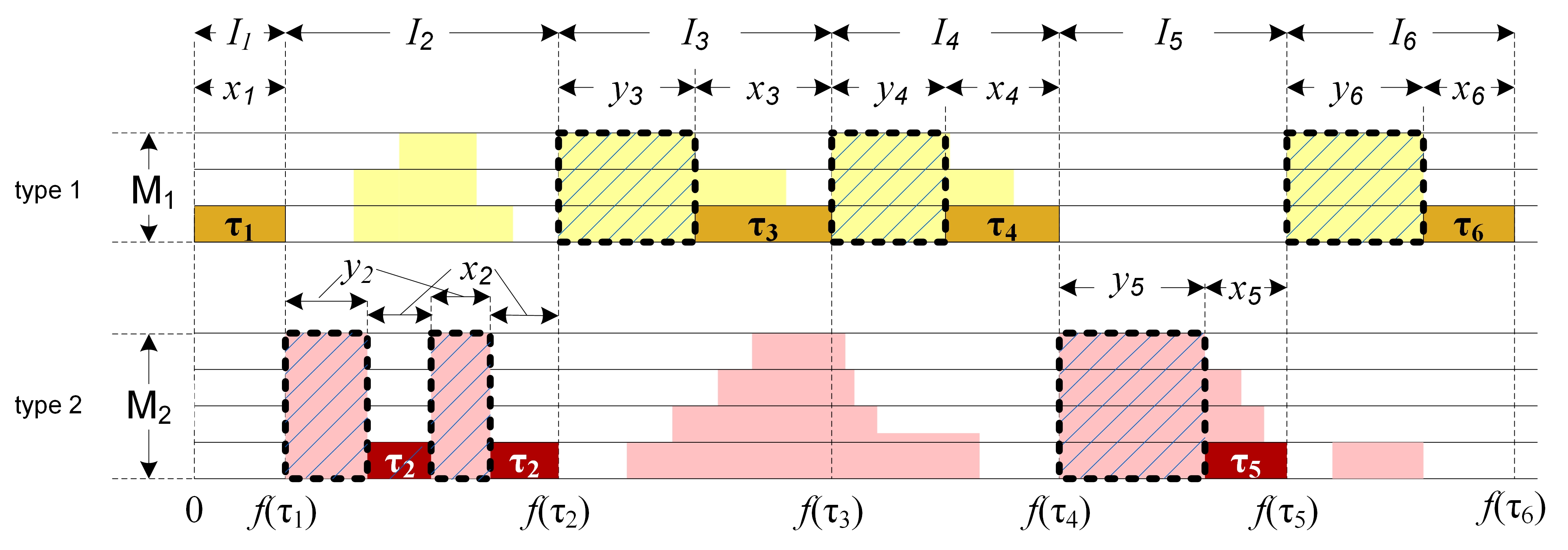
Figure 3: Illustration of $x_{i}$, $y_{i}$ and $I_{i}$.

Obviously, $I_{i}=x_{i}+y_{i}$. Figure 3 illustrates $x_{i}$, $y_{i}$ and $I_{i}$. In general the time intervals counted in $x_{i}$ or $y_{i}$ may not be continuous (e.g., $[f(\tau_{1}),f(\tau_{2}))$ in Figure 3). We further define

$$\mathcal{I}_{s}=\sum_{\begin{subarray}{c}\tau_{i}\in\pi\wedge\\ \gamma(\tau_{i})=s\end{subarray}}I_{i},~{}~{}\mathcal{X}_{s}=\sum_{\begin{subarray}{c}\tau_{i}\in\pi\wedge\\ \gamma(\tau_{i})=s\end{subarray}}x_{i},~{}~{}\mathcal{Y}_{s}=\sum_{\begin{subarray}{c}\tau_{i}\in\pi\wedge\\ \gamma(\tau_{i})=s\end{subarray}}y_{i},$$

and we know $\mathcal{I}_{s}=\mathcal{X}_{s}+\mathcal{Y}_{s}$.

      Lemma 3.1.

Let $\pi=\{\tau_{1},\cdots,\tau_{k}\}$ be a critical path of an arbitrary execution sequence of $G$, then $\mathcal{X}_{s}$ and $\mathcal{Y}_{s}$ can be bounded by

$$\mathcal{X}_{s} \leq\sum_{\begin{subarray}{c}\tau_{j}\in\pi\wedge\\ \gamma(\tau_{j})=s\end{subarray}}c(\tau_{j}),$$ (2)

$$\mathcal{Y}_{s} \leq\left(vol_{s}(G)-\sum_{\begin{subarray}{c}\tau_{j}\in\pi\wedge\\ \gamma(\tau_{j})=s\end{subarray}}c(\tau_{j})\right)/M_{s}.$$ (3)

Proof.

The proof of (2) is trivial. In the following, we focus on the proof of (3). By the definition of critical path, we know all the predecessors of $\tau_{i}$ have finished by time $f(\tau_{i-1})$. Therefore, when $\tau_{i}$ is not executing in $[f(\tau_{i-1}),f(\tau_{i}))$, all the cores of type $\gamma(\tau_{i})$ must be occupied by vertices of type $\gamma(\tau_{i})$ not on the critical path. Since the total workload of vertices of type $s$ that are not on the critical path is at most

$$vol_{s}(G)-\sum_{\begin{subarray}{c}\tau_{j}\in\pi\wedge\\ \gamma(\tau_{j})=s\end{subarray}}c(\tau_{j})$$

and the number of cores of type $s$ is $M_{s}$, the accumulated length of time intervals during which the vertices of type $s$ on $\pi$ are not executing is bounded by (3). ∎

      Theorem 3.1 (NEW-B-1).

The WCRT of $G$ is bounded by:

$$R(G)\leq len(\hat{G})+\sum_{s\in S}\frac{vol_{s}(G)}{M_{s}},\vspace{-2mm}$$ (4)

where $\hat{G}$ is the scaled graph of $G$.

Proof.

By (2), (3) and $\mathcal{I}_{s}=\mathcal{X}_{s}+\mathcal{Y}_{s}$ we have

$$\mathcal{I}_{s} \leq\frac{vol_{s}(G)}{M_{s}}+\sum_{\begin{subarray}{c}\tau_{i}\in\pi\wedge\\ \gamma(\tau_{i})=s\end{subarray}}\left(1-1/M_{s}\right)c(\tau_{i})$$

$$\sum_{s\in S}\mathcal{I}_{s} \leq\sum_{s\in S}\frac{vol_{s}(G)}{M_{s}}+\sum_{s\in S}\sum_{\begin{subarray}{c}\tau_{i}\in\pi\wedge\\ \gamma(\tau_{i})=s\end{subarray}}\left(1-1/M_{s}\right)c(\tau_{i})$$

$$\sum_{s\in S}\mathcal{I}_{s} \leq\sum_{s\in S}\frac{vol_{s}(G)}{M_{s}}+\sum_{\begin{subarray}{c}\tau_{i}\in\pi\end{subarray}}\hat{c}(\tau_{i})~{}\emph{{//by the definition of~{}}}\hat{c}(\tau_{i})$$

$\sum_{s\in S}\mathcal{I}_{s}$ is the response time of the execution sequence with critical path $\pi$. Since $G$ and $\hat{G}$ have the same topology, $\pi$ is also a complete path in $\hat{G}$, so $\sum_{\begin{subarray}{c}\tau_{i}\in\pi\end{subarray}}\hat{c}(\tau_{i})$ is bounded by $len(\hat{G})$. Therefore, $R(G)$ is bounded by (4). ∎

We can compute $\sum_{s\in S}vol_{s}(G)/M_{s}$ and construct $\hat{G}$ based on $G$ in $O(|V|)$ time, and compute $len(\hat{G})$ in $O(|V|+|E|)$ time [11]. Therefore, the overall time complexity to compute NEW-B-1 is $O(|V|+|E|)$, which is the same as OLD-B-1. By comparing the two bounds we can conclude:

      Corollary 3.1.

NEW-B-1 strictly dominates OLD-B-1.

Finally, we can easily see the bound in (4) is decreasing with respect to each $M_{s}$, so we can conclude:

      Corollary 3.2.

NEW-B-1 is self-sustainable with respect to each $M_{s}$.

4 The Second New WCRT Bound

Our first new WCRT bound NEW-B-1 is more precise than OLD-B, but still very pessimistic. The source of its pessimism comes from the step of bounding $\mathcal{Y}_{s}$. Intuitively, the bound of $\mathcal{Y}_{s}$ in (3) is derived assuming that the workload of vertices not on the critical path are all executed in the shaded areas in Figure 3. However, in reality much workload of $G$ may actually be executed outside these shaded areas. Therefore, the length of $\mathcal{Y}_{s}$ is significantly over-estimated in (3) .

In this section, we introduce the second new WCRT bound NEW-B-2, which eliminates workload of vertices that cannot be executed in the shaded area, and thus reduce the pessimism in bounding $\mathcal{Y}_{s}$.

4.1 WCRT Bound

      Definition 4.1.

For each vertex $v\in V$, $\textsf{{par}}(v)$ denotes the set of vertices that have the same type as $v$ but are neither ancestors nor descendants of $v$:

$$\textsf{{par}}(v)=\{u|{u\in V}\wedge{\gamma(u)=\gamma(v)}\wedge{u\notin(\textsf{{ans}}(v)\cup\textsf{{des}}(v))}\}.$$

      Definition 4.2.

Let $\pi=\{\tau_{1},\cdots,\tau_{k}\}$ be a critical path, $\textsf{{ivs}}(\pi,s)$ is defined as

$$\textsf{{ivs}}(\pi,s)=\bigcup_{\begin{subarray}{c}\tau_{i}\in\pi\wedge\\ \gamma({\tau_{i}})=s\end{subarray}}\textsf{{par}}(\tau_{i}).$$ (5)

      Example 4.1.

Assume $\pi=\{v_{0},v_{1},v_{7},v_{11},v_{12}\}$ is a critical path of the task in Figure 1. We have $\textsf{{par}}(v_{0})=\emptyset$, $\textsf{{par}}(v_{1})=\{v_{2},v_{4},v_{5},v_{8},v_{9},v_{10}\}$, $\textsf{{par}}(v_{7})=\{v_{6}\}$, $\textsf{{par}}(v_{11})=\{v_{4},v_{5},v_{8},v_{9},v_{10}\}$, $\textsf{{par}}(v_{12})=\emptyset$, $\textsf{{ivs}}(\pi,1)=\{v_{6}\}$ and $\textsf{{ivs}}(\pi,2)=\{v_{2},v_{4},v_{5},v_{8},v_{9},v_{10}\}$.

Intuitively, $\textsf{{ivs}}(\pi,s)$ is the set of vertices of type $s$ that are not on the critical path but can actually interfere with vertices of type $s$ on the critical path (i.e., can be executed in the shaded area in Figure 3). Therefore, $\mathcal{Y}_{s}$ can be bounded more precisely as stated in the following Lemma.

      Lemma 4.1.

Let $\pi=\{\tau_{1},\cdots,\tau_{k}\}$ be a critical path of an arbitrary execution sequence of $G$, then $\mathcal{Y}_{s}$ is bounded by

$$\mathcal{Y}_{s}\leq\frac{\textsf{{ivs}}(\pi,s)}{M_{s}}$$ (6)

Proof.

To prove the lemma, it is sufficient to prove that at any time instant in $[f(\tau_{i-1}),f(\tau_{i}))$ when $\tau_{i}$ is not executing, all the cores of type $\gamma(\tau_{i})$ must be executing vertices in $\textsf{{ivs}}(\pi,\gamma(\tau_{i}))$. We prove this by contradiction. Assuming that at a time instant $t\in[f(\tau_{i-1}),f(\tau_{i}))$ when $\tau_{i}$ is not executing, there exists a core of type $\gamma(\tau_{i})$ which is not executing vertices in $\textsf{{ivs}}(\pi,\gamma(\tau_{i}))$, then one of the following two cases must be true:

• This core is idle at $t$. Since $\pi$ is a critical path, we know all the predecessors of $\tau_{i}$ have finished by time $f(\tau_{i-1})$, so $\tau_{i}$ is eligible for execution at $t$, and thus this core cannot be idle at $t$. Therefore, this case is impossible.

• This core is executing a vertex $u\notin\textsf{{ivs}}(\pi,\gamma(\tau_{i}))$ at $t$. First we know $\gamma(u)=\gamma(\tau_{i})$, and since $u\notin\textsf{{ivs}}(\pi,\gamma(\tau_{i}))$, by the definition of ivs we know $u$ must be a predecessor or a successor of $\tau_{i}$, so we discuss two cases:

  • $u$ is a predecessor of $\tau_{i}$. Since $\pi$ is a critical path, we know all the predecessors of $\tau_{i}$ have finished by time $f(\tau_{i-1})$, so a predecessor of $\tau_{i}$ cannot start execution after $f(\tau_{i-1})$, which contradicts that $u$ is executing at a time instant $t$ after $f(\tau_{i-1})$.

  • $u$ is a successor of $\tau_{i}$. A successor of $\tau_{i}$ cannot start execution before $f(\tau_{i})$, so this is also a contradiction.

  Therefore, this case is also impossible.

In summary, both cases are impossible, so the assumption must be false and the lemma is proved. ∎

      Theorem 4.1 (NEW-B-2).

The WCRT of $G$ is bounded by

$$R(G)\leq\max_{\pi\in G}\{\widetilde{R}(\pi)\}$$ (7)

where

$$\widetilde{R}(\pi)=len(\pi)+\sum_{s\in S}\sum_{v\in\textsf{{ivs}}(\pi,s)}c(v)/M_{s}$$ (8)

Proof.

By the same idea as the proof of Theorem 3.1 but using the new bound (6) for $\mathcal{Y}_{s}$ instead of (3), we can get

$$\sum_{s\in S}\mathcal{I}_{s}\leq len(\pi)+\sum_{s\in S}\sum_{v\in\textsf{{ivs}}(\pi,s)}c(v)/M_{s}$$

$\sum_{s\in S}\mathcal{I}_{s}$ is the response time of the execution sequence with $\pi$ being the critical path. Finally, by getting the maximum bound for all complete paths (assumed to be the critical path), the theorem is proved. ∎

Comparing with NEW-B-1, NEW-B-2 uses a more precise upper bound of $\mathcal{Y}_{s}$, so we have

      Corollary 4.1.

NEW-B-2 strictly dominates NEW-B-1.

The bound in (7) is decreasing with respect to each $M_{s}$, so

      Corollary 4.2.

NEW-B-2 is self-sustainable with respect to each $M_{s}$.

4.2 Strong NP-Hardness

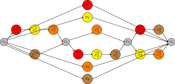
Figure 4: The constructed typed DAG task $G$ for 3-SAT problem instance $\mathcal{C}=\mathcal{C}_{1}\wedge\mathcal{C}_{2}\wedge\mathcal{C}_{3}\wedge\mathcal{C}_{4}$, where $\mathcal{C}_{1}=x_{1}\vee\overline{x_{2}}\vee x_{3}$, $\mathcal{C}_{2}=x_{1}\vee\overline{x_{2}}\vee\overline{x_{3}}$, $\mathcal{C}_{3}=x_{1}\vee x_{2}\vee\overline{x_{3}}$, $\mathcal{C}_{4}=\overline{x_{1}}\vee\overline{x_{2}}\vee x_{3}$.

NEW-B-2 requires to compute the maximum of $\widetilde{R}(\pi)$ among all paths in the graph $G$. It is computationally intractable to explicitly enumerate all the paths, the number of which is exponential. Can we develop efficient algorithms of (pseudo-)polynomial complexity to compute $\max_{\pi\in G}\{\widetilde{R}(\pi)\}$?

Unfortunately, this is impossible unless P = NP.

      Theorem 4.2.

The problem of computing $\max_{\pi\in G}\{\widetilde{R}(\pi)\}$ is strongly NP-hard.

Proof.

We will prove the theorem by showing that even a simpler problem of verifying whether $\max_{\pi\in G}\{\widetilde{R}(\pi)\}$ is larger than a given value $\omega$ is strongly NP-hard, which is proved by a reduction from the 3-SAT problem.

Let $\mathcal{C}$ be an arbitrary instance of the 3-SAT problem, which has $m$ clauses $\mathcal{C}_{1}\bigwedge\mathcal{C}_{2}\bigwedge\cdots\bigwedge\mathcal{C}_{m}$ and $n$ variables $\{x_{1},x_{2},\cdots,x_{n}\}$. Each clause $\mathcal{C}_{r}$, $1\leq r\leq m$, consists of three literals, and each literal is a variable or the negation of a variable. We construct a typed DAG $G$ corresponding to the 3-SAT instance as follows:

• We first construct $n+1$ vertices $\{v_{0},\cdots,v_{n}\}$ of type $s_{0}$ with $c(v_{0})=\cdots=c(v_{n})=1$. $v_{0}$ is the source vertex of $G$ and $v_{n}$ is the sink vertex.

• For each clause $\mathcal{C}_{r}$, we construct a vertex $u_{r}$ of type $s_{r}$ with $c(u_{r})=1$, as well as two edges $(v_{0},u_{r})$ and $(u_{r},v_{n})$.

• For each variable $x_{i}$, we construct two paths from $v_{i-1}$ to $v_{i}$:

  • Positive path, which includes a vertex $x_{i}^{r}$ of type $s_{r}$ if and only if clause $\mathcal{C}_{r}$ includes a literal $x_{i}$.

  • Negative path, which includes a vertex $\overline{x_{i}^{r}}$ if and only if clause $\mathcal{C}_{r}$ includes a literal $\overline{x_{i}}$.

  The WCET of each vertex on these two paths is $\frac{1}{mn+1}$.

Note that there are in total $m+1$ types in the above constructed DAG. Finally, we set $M_{0}=M_{1}=\cdots=M_{m}=1$ and $\omega=m+n+1$. The above construction is polynomial as there are no more than $m+n+1+2nm$ vertices in the constructed graph. For illustration, an example of the above construction is given in Figure 4.

In the following we prove that the 3-SAT problem instance $\mathcal{C}$ is satisfiable if and only if the bound $\max_{\pi\in G}\{\widetilde{R}(\pi)\}$ of the above constructed graph is strictly greater than $m+n+1$.

First, a complete path that leads to the largest $\widetilde{R}(\pi)$ must be one of those traversing $v_{0},\cdots,v_{n}$. The choice between the positive and negative path between $v_{i-1}$ and $v_{i}$ corresponds to the choice between assigning $1$ or $0$ to variable $x_{i}$ in the 3-SAT problem.

Since each vertex $u_{r}$ is neither an ancestor nor a descendant of any vertex on paths traversing $v_{0},\cdots,v_{n}$, $u_{r}$ is included in $\textsf{{ivs}}(\pi,\gamma(u_{r}))$ if and only if the path $\pi$ contains at least one vertex of type $\gamma(u_{r})$. This corresponds to that $\mathcal{C}_{r}$ is satisfied only if it contains at least one literal assigned with value $1$. Therefore, we can conclude that all vertices $u_{r}$ are included in the corresponding $\textsf{{ivs}}(\pi,\gamma(u_{r}))$ if and only if all clauses contain at least one literal assigned with value $1$, i.e., the 3-SAT problem instance $\mathcal{C}$ is satisfiable.

Therefore, the second item of RHS of (8) equals $m$ if and only if $\mathcal{C}$ is satisfiable. Moreover, there are at most $mn$ vertices corresponding to the positive and negative values of the variables along any path traversing $v_{0},\cdots,v_{n}$, so their total WCET must be in the range $(0,\frac{mn}{mn+1})$. Therefore, the length $len(\pi)$ of any such path $\pi$ must be in the range $(n+1,n+1+\frac{mn}{mn+1})$, and thus in the range $(n+1,n+2)$. Therefore, $\max_{\pi\in G}$ is larger than $m+n+1$ if and only if all vertices $u_{r}$ are included in the corresponding $\textsf{{ivs}}(\pi,\gamma(u_{r}))$, i.e., the 3-SAT problem instance $\mathcal{C}$ is satisfiable. ∎

4.3 Computation Algorithm

The construction in the above strong NP-hardness proof uses $m+1$ different types (where $m$ is the number of clauses in 3-SAT). In realistic heterogeneous multi-core platforms, the number of core types is usually not very large. Will the problem of computing $\max_{\pi\in G}\{\widetilde{R}(\pi)\}$ remain NP-hard if the number of types is a bounded constant? In the following, we will present an algorithm to compute $\max_{\pi\in G}\{\widetilde{R}(\pi)\}$ with complexity ${O(|V|^{|S|+2})}$, which shows that the problem is actually in P if the number of types is a constant.

We first describe the intuition of our algorithm. Instead of explicitly enumerating all the possible paths, our algorithm will use abstractions to represent paths in the graph searching procedure. More specifically, a path starting from the source vertex of $G$ and ending at some vertex $\tau_{i}$ is abstractly represented by a tuple $\langle\tau_{i},\Delta(\tau_{i}),\mathcal{R}(\tau_{i})\rangle$, where $\Delta(\tau_{i})$ and $\mathcal{R}(\tau_{i})$ are defined in Definition 4.3 and 4.4 in the following. The tuple will be updated when the path is extended from $\tau_{i}$ to its successor $\tau_{i+1}$, and eventually when the path is extended to the sink vertex, $\mathcal{R}(\tau_{i})$ is the $\widetilde{R}(\pi)$ for this path. The algorithm starts with a single tuple corresponding to the path consisting only the source vertex and repeatedly extends the paths until they all reach the sink vertex, then the maximal $\widetilde{R}(\pi)$ among all the kept tuples is the desired bound $\max_{\pi\in G}\{\widetilde{R}(\pi)\}$. The abstraction is compact, so that many different path histories ending with the same vertex can be represented by a single abstraction and the total number of abstractions generated in the computation is polynomially bounded.

      Definition 4.3.

For a path $\pi=\{\tau_{1},\cdots,\tau_{k}\}$ in $G$ and a type $s\in S$, we define

$$\delta(\tau_{i},s)=\begin{cases}\tau_{i},&s=\gamma(\tau_{i})\\ \bot,&s\neq\gamma(\tau_{1})\wedge i=1\\ \delta(\tau_{i\textrm{-}1},s),&s\neq\gamma(\tau_{i})\wedge 2\leq i\leq k\end{cases}$$

and

$$\Delta(\tau_{i})=\{\delta(\tau_{i},s)~{}|~{}s\in S\}$$ (9)

Intuitively, $\delta(\tau_{i},s)$ is the vertex on path $\pi$ that is the closest to $\tau_{i}$ among all the vertices of type $s$.

      Example 4.2.

In the typed task in Figure 1, there are $3$ paths from $v_{0}$ to $v_{7}$. For the path $\pi_{1}=\{v_{0},v_{1},v_{7}\}$, one can derive $\delta(v_{7},1)=\{v_{7}\}$ and $\delta(v_{7},2)=\{v_{1}\}$. For the path $\pi_{2}=\{v_{0},v_{3},v_{7}\}$, one can derive $\delta(v_{7},1)=\{v_{7}\}$ and $\delta(v_{7},2)=\{v_{0}\}$.

      Definition 4.4.

For a path $\pi=\{\tau_{1},\cdots,\tau_{k}\}$ in $G$ we define:

$$\mathcal{R}(\tau_{i})=\begin{cases}c(\tau_{1}),&i=1\\ \displaystyle\mathcal{R}(\tau_{i\textrm{-}1})+c(\tau_{i})+\!\!\sum_{v\in\varphi(\tau_{i})}\frac{c(v)}{M_{\gamma(\tau_{i})}},&2\leq i\leq k\end{cases}$$ (10)

where

$$\varphi(\tau_{i})=\textsf{{par}}(\tau_{i})\setminus\textsf{{par}}(\delta(\tau_{i\textrm{-}1}))$$

(since $\delta(\tau_{i\textrm{-}1})$ may be $\bot$, we let $\textsf{{par}}(\bot)=\emptyset$ for completeness).

      Lemma 4.2.

For a complete path $\pi=\{\tau_{1},\cdots,\tau_{k}\}$, it always holds

$$\mathcal{R}(\tau_{k})=\widetilde{R}(\pi).$$ (11)

Proof.

The proof goes in two steps: (1) Rewrite $\mathcal{R}(\tau_{i})$ into a non-recursive form $\mathcal{R}^{\prime}(\tau_{i})$ and prove $\forall\tau_{i}\in\pi:\mathcal{R}^{\prime}(\tau_{i})=\mathcal{R}(\tau_{i})$, and (2) Prove $\mathcal{R}^{\prime}(\tau_{k})=\widetilde{R}(\pi)$.

We first define $\mathcal{R}^{\prime}(\tau_{i})$ as follows:

$$\mathcal{R}^{\prime}(\tau_{i})=\left\{\begin{array}[]{ll}c(\tau_{1})&i=1\\ \displaystyle\sum_{j=1}^{i}c(\tau_{j})+\sum_{s\in S}\sum_{\begin{subarray}{c}v\in\varphi(\tau_{j})\wedge\\ \gamma(\tau_{j})=s\wedge j\leq i\end{subarray}}\frac{c(v)}{M_{s}}&2\leq i\leq k\end{array}\right.$$

Now we prove $\forall\tau_{i}\!\in\!\pi\!:\mathcal{R}^{\prime}(\tau_{i})=\mathcal{R}(\tau_{i})$ by induction:

• Base case. Both $\mathcal{R}(\tau_{1})$ and $\mathcal{R}^{\prime}(\tau_{1})$ equal $c(\tau_{1})$, so the claim holds for the base case with $i=1$.

• Inductive step. Suppose $\mathcal{R}(\tau_{i\textrm{-}1})=\mathcal{R}^{\prime}(\tau_{i\textrm{-}1})$, we want to prove $\mathcal{R}(\tau_{i})=\mathcal{R}^{\prime}(\tau_{i})$. First, we know

  $$\!\!\!\!\!\!\!\!\!\!\!\!\!\!\sum_{v\in\varphi(\tau_{i})}\frac{c(v)}{M_{\gamma(\tau_{i})}}+\sum_{s\in S}\!\!\!\!\sum_{\begin{subarray}{c}v\in\varphi(\tau_{j})\wedge\\ \gamma(\tau_{j})=s\wedge j\leq i-1\end{subarray}}\!\!\!\!\!\!\!\!\frac{c(v)}{M_{s}}=\sum_{s\in S}\!\!\sum_{\begin{subarray}{c}v\in\varphi(\tau_{j})\wedge\\ \gamma(\tau_{j})=s\wedge j\leq i\end{subarray}}\!\!\!\!\!\frac{c(v)}{M_{s}}$$ (12)

  For simplicity we let

  $$\mathcal{F}(\tau_{i})=\sum_{s\in S}\!\!\sum_{\begin{subarray}{c}v\in\varphi(\tau_{j})\wedge\\ \gamma(\tau_{j})=s\wedge j\leq i\end{subarray}}\!\!\!\!\!\frac{c(v)}{M_{s}}$$

  so (12) can be rewritten as

  $$\sum_{v\in\varphi(\tau_{i})}\frac{c(v)}{M_{\gamma(\tau_{i})}}+\mathcal{F}(\tau_{i\textrm{-}1})=\mathcal{F}(\tau_{i})$$

  $$\Leftrightarrow\!\! \sum_{v\in\varphi(\tau_{i})}\!\!\!\frac{c(v)}{M_{\gamma(\tau_{i})}}\!+\!\mathcal{F}(\tau_{i\textrm{-}1})\!+\!\!\sum_{j=1}^{i}c(\tau_{j})=\mathcal{F}(\tau_{i})\!+\!\!\sum_{j=1}^{i}c(\tau_{j})$$

  $$\Leftrightarrow\!\! \sum_{v\in\varphi(\tau_{i})}\frac{c(v)}{M_{\gamma(\tau_{i})}}+\mathcal{R}^{\prime}(\tau_{i\textrm{-}1})+c(\tau_{i})=\mathcal{R}^{\prime}(\tau_{i})$$

  $$\Leftrightarrow\!\! \sum_{v\in\varphi(\tau_{i})}\frac{c(v)}{M_{\gamma(\tau_{i})}}+\mathcal{R}(\tau_{i\textrm{-}1})+c(\tau_{i})=\mathcal{R}^{\prime}(\tau_{i})$$

  $$\Leftrightarrow\!\! ~{}~{}~{}\mathcal{R}(\tau_{i})=\mathcal{R}^{\prime}(\tau_{i})$$

By now, we have proved $\forall\tau_{i}\in\pi:\mathcal{R}^{\prime}(\tau_{i})=\mathcal{R}(\tau_{i})$. In the following we prove $\mathcal{R}^{\prime}(\tau_{k})=\widetilde{R}(\pi)$.

Let $\pi^{s}=\{\tau^{s}_{1},\cdots,\tau^{s}_{h}\}$ be the subsequence of $\pi$ containing all vertices in $\pi$ with type $s$. By the definition of $\varphi({\tau_{j}})$:

$$\sum_{\begin{subarray}{c}v\in\varphi({\tau_{j}})\\ \wedge\gamma({\tau_{j}})=s\\ \wedge j\leq k\end{subarray}}\!\!\!\!c(v)=\!\!\!\!\!\!\sum_{v\in\textsf{{par}}(\tau^{s}_{1})}\!\!\!\!c(v)+\!\!\!\!\sum_{\begin{subarray}{c}v\in\textsf{{par}}(\tau^{s}_{2})\\ \setminus\textsf{{par}}(\tau^{s}_{1})\end{subarray}}\!\!\!\!c(v)+\cdots+\!\!\!\!\sum_{\begin{subarray}{c}v\in\textsf{{par}}(\tau^{s}_{h})\\ \setminus\textsf{{par}}(\tau^{s}_{h\textrm{-}1})\end{subarray}}\!\!\!\!c(v)$$ (13)

In the following we will prove

$$\sum_{v\in\textsf{{ivs}}(\pi,s)}\!\!\!\!c(v)=\!\!\!\!\!\!\sum_{v\in\textsf{{par}}(\tau^{s}_{1})}\!\!\!\!c(v)+\!\!\!\!\sum_{\begin{subarray}{c}v\in\textsf{{par}}(\tau^{s}_{2})\\ \setminus\textsf{{par}}(\tau^{s}_{1})\end{subarray}}\!\!\!\!c(v)+\cdots+\!\!\!\!\sum_{\begin{subarray}{c}v\in\textsf{{par}}(\tau^{s}_{h})\\ \setminus\textsf{{par}}(\tau^{s}_{h\textrm{-}1})\end{subarray}}\!\!\!\!c(v)$$ (14)

If (14) is true, then by (14) and (13) we have

$$\sum_{\begin{subarray}{c}v\in\varphi({\tau_{j}})\\ \wedge\gamma({\tau_{j}})=s\\ \wedge j\leq k\end{subarray}}c(v)=\sum_{v\in\textsf{{ivs}}(\pi,s)}c(v)$$

by which $\mathcal{R}^{\prime}(\tau_{k})=\widetilde{R}(\pi)$ is proved.

In the following, we focus on proving (14). We use LHS and RHS to represent the left-hand side and right-hand side of (14), respectively. In the following, we will prove that both LHS $\leq$ RHS and LHS $\geq$ RHS hold.

1. LHS $\leq$ RHS. This is proved by combining the following two claims:

   1. Any $c(v)$ counted in LHS is also counted in RHS. If $c(v)$ is counted in LHS, then $v$ must be in some $\textsf{{par}}(\tau_{i}^{s})$, and by the definition of $\textsf{{ivs}}(\pi,s)$, we know $v$ must be also in $\textsf{{ivs}}(\pi,s)$, so we can conclude that all the $c(v)$ counted in LHS are also counted in RHS.

   2. Each $c(v)$ is counted in LHS at most once. Suppose this is not true, then there exists some $v$ such that $v\in\textsf{{par}}(\tau^{s}_{i})\setminus\textsf{{par}}(\tau^{s}_{i\textrm{-}1})$ and $v\in\textsf{{par}}(\tau^{s}_{j})\setminus\textsf{{par}}(\tau^{s}_{j\textrm{-}1})$ for some $j<i-1$, so it must be the case that

      $$v\in\textsf{{par}}(\tau^{s}_{i})~{}\wedge~{}v\notin\textsf{{par}}(\tau^{s}_{i\textrm{-}1})~{}\wedge~{}v\in\textsf{{par}}(\tau^{s}_{j})$$

      By $v\in\textsf{{par}}(\tau^{s}_{i})$, we know $v$ is not a descendant of $\tau^{s}_{i}$, and since $\tau^{s}_{i\textrm{-}1}$ is a predecessor of $\tau^{s}_{i}$, $v$ is not a descendant of $\tau^{s}_{i\textrm{-}1}$ either. On the other hand, by $v\in\textsf{{par}}(\tau^{s}_{j})$ we know $v$ is not an ancestor of $\tau^{s}_{j}$, and since $\tau^{s}_{i\textrm{-}1}$ is a descendant of $\tau^{s}_{j}$, $v$ is not an ancestor of $\tau^{s}_{i-1}$. In summary, $v$ is neither a descendant nor an ancestor of $\tau^{s}_{i\textrm{-}1}$, and $v$ has the same type as $\tau^{s}_{i\textrm{-}1}$, which contradicts $v\notin\textsf{{par}}(\tau^{s}_{i\textrm{-}1})$.

2. RHS $\leq$ LHS. It is obvious that each $c(v)$ is counted at most once in the RHS, so it suffices to prove that each $c(v)$ counted in the RHS is also counted in LHS. Since $v\in\textsf{{ivs}}(\pi,s)$, $v$ must be in some $\textsf{{par}}(\tau_{i}^{s})$. Suppose $i$ is the smallest index such that $v\in\textsf{{par}}(\tau_{i}^{s})$ but $v\notin\textsf{{par}}(\tau_{i-1}^{s})$, then $c(v)$ is counted in item $\sum_{v\in\textsf{{par}}(\tau^{s}_{i})-\textsf{{par}}(\tau^{s}_{i\textrm{-}1})}c(v)$ (if $i=1$ then $c(v)$ is counted in $\sum_{v\in\textsf{{par}}(\tau^{s}_{1})}c(v)$).

In summary, we have proved both RHS $\geq$ LHS and RHS $\leq$ LHS, so (14) is true. ∎

By Lemma 4.2, we know that by using the abstract tuple $\langle\tau_{i},\Delta(\tau_{i}),\mathcal{R}(\tau_{i})\rangle$ to extend the path, eventually, we can precisely compute $\widetilde{R}(\pi)$. Therefore, we can use $\langle\tau_{i},\Delta(\tau_{i}),\mathcal{R}(\tau_{i})\rangle$ as the abstraction of paths to perform graph searching. All the paths corresponding to the same tuple can be abstractly represented by a single tuple instead of recording each of them individually. Actually, even paths corresponding to different tuples can be merged together during the graph searching procedure by the domination relation among tuples defined as follows:

      Definition 4.5.

Given two tuples $\langle v,\Delta_{1}(v),\mathcal{R}_{1}(v)\rangle$ and $\langle v,\Delta_{2}(v),\mathcal{R}_{2}(v)\rangle$ with the same vertex $v$, $\langle v,\Delta_{1}(v),\mathcal{R}_{1}(v)\rangle$ dominates $\langle v,\Delta_{2}(v),\mathcal{R}_{2}(v)\rangle$, denoted by

$$\langle v,\Delta_{1}(v),\mathcal{R}_{1}(v)\rangle\succcurlyeq\langle v,\Delta_{2}(v),\mathcal{R}_{2}(v)\rangle,$$

if both of the following conditions are satisfied:

1. $\mathcal{R}_{1}(v)\geq\mathcal{R}_{2}(v)$

2. $\forall s$: either $\delta_{1}(v,s)=\bot$ or

   $$(\delta_{1}(v,s)\!\neq\!\bot)~{}\wedge~{}(\delta_{2}(v,s)\!\neq\!\bot)~{}\wedge~{}$$

   $$~{}~{}~{}~{}~{}~{}~{}~{}~{}~{}~{}~{}~{}~{}~{}~{}~{}~{}~{}~{}~{}(\textsf{{par}}(\delta_{1}(v,s))\cap\textsf{{des}}(\delta_{2}(v,s))\!=\!\emptyset)$$

Suppose $v$ is a successor of $u$. Given a tuple $\langle u,\Delta(u),\mathcal{R}(u)\rangle$ for vertex $u$ and a tuple $\langle v,\Delta(v),\mathcal{R}(v)\rangle$ for vertex $v$, we use

$$\langle u,\Delta(u),\mathcal{R}(u)\rangle\mapsto\langle v,\Delta(v),\mathcal{R}(v)\rangle$$

to denote that $\langle v,\Delta(v),\mathcal{R}(v)\rangle$ is generated based on $\langle u,\Delta(u),\mathcal{R}(u)\rangle$ according to (9) and (10).

      Lemma 4.3.

Suppose $v$ is a successor of $u$, and

$$\langle u,\Delta_{1}(u),\mathcal{R}_{1}(u)\rangle \mapsto\langle v,\Delta_{1}(v),\mathcal{R}_{1}(v)\rangle$$

$$\langle u,\Delta_{2}(u),\mathcal{R}_{2}(u)\rangle \mapsto\langle v,\Delta_{2}(v),\mathcal{R}_{2}(v)\rangle$$

if $\langle u,\Delta_{1}(u),\mathcal{R}_{1}(u)\rangle\succcurlyeq\langle u,\Delta_{2}(u),\mathcal{R}_{2}(u)\rangle$, then we must have $\langle v,\Delta_{1}(v),\mathcal{R}_{1}(v)\rangle\succcurlyeq\langle v,\Delta_{2}(v),\mathcal{R}_{2}(v)\rangle$.

Proof.

We start with proving $\mathcal{R}_{1}(v)\geq\mathcal{R}_{2}(v)$. Assume $w_{1}=\delta_{1}(u,\gamma(v))$ and $w_{2}=\delta_{2}(u,\gamma(v))$, then

$$\varphi_{1}(v)=\textsf{{par}}(v)\setminus\textsf{{par}}(w_{1})$$

$$\varphi_{2}(v)=\textsf{{par}}(v)\setminus\textsf{{par}}(w_{2})$$

In the following we prove $\varphi_{1}(v)\supseteq\varphi_{2}(v)$. By condition 2) in Definition 4.5, one of the following two cases must hold

1. $w_{1}=\bot$

2. $(w_{1}\!\neq\!\bot)~{}\wedge~{}(w_{2}\!\neq\!\bot)~{}\wedge~{}(\textsf{{par}}(w_{1})\cap\textsf{{des}}(w_{2})\!=\!\emptyset)$

If $w_{1}=\bot$, then $\textsf{{par}}(w_{1})=\emptyset$, so $\varphi_{1}(v)\supseteq\varphi_{2}(v)$ is obviously true. In the following we focus on the second case

$$(w_{1}\!\neq\!\bot)~{}\wedge~{}(w_{2}\!\neq\!\bot)~{}\wedge~{}(\textsf{{par}}(w_{1})\cap\textsf{{des}}(w_{2})\!=\!\emptyset).$$

Suppose $\varphi_{1}(v)\nsupseteq\varphi_{2}(v)$ , then there must exist an $x$ s.t.

$$x\in\varphi_{2}(v)\wedge x\notin\varphi_{1}(v),$$

by which we know any following conditions must hold

$$x \in\textsf{{par}}(v)$$ (15)

$$x \in\textsf{{par}}(w_{1})$$ (16)

$$x \notin\textsf{{par}}(w_{2})$$ (17)

By (15) we have $x\notin\textsf{{ans}}(v)\cup\textsf{{des}}(v)$ and thus

$$x\notin\textsf{{ans}}(v)$$ (18)

By (17), we have

$$x\in\textsf{{ans}}(w_{2})\cup\textsf{{des}}(w_{2}).$$ (19)

Since $w_{2}=\delta_{2}(u,\gamma(v))$ and $v\in\textsf{{suc}}(u)$, we know $w_{2}\in\textsf{{ans}}(v)$, and thus

$$\textsf{{ans}}(w_{2})\subset\textsf{{ans}}(v)$$ (20)

By (18), (19) and (20) we know $x\in\textsf{{des}}(w_{2})$, which contradicts with $\textsf{{par}}(w_{1})\cap\textsf{{des}}(w_{2})=\emptyset$, so the assumption $\varphi_{1}(v)\nsupseteq\varphi_{2}(v)$ must be false, i.e., $\varphi_{1}(v)\supseteq\varphi_{2}(v)$ must be true. Therefore

$$\sum_{w\in\varphi_{1}(v)}\frac{c(w)}{M_{\gamma(v)}}\geq\sum_{w\in\varphi_{2}(v)}\frac{c(w)}{M_{\gamma(v)}},$$

and since $\mathcal{R}_{1}(u)\geq\mathcal{R}_{2}(u)$ , we have

$$\mathcal{R}_{1}(u)+c(v)+\sum_{w\in\varphi_{1}(v)}\frac{c(w)}{M_{\gamma(v)}}\geq\mathcal{R}_{1}(u)+c(v)\sum_{w\in\varphi_{2}(v)}\frac{c(w)}{M_{\gamma(v)}}$$

by which we have $\mathcal{R}_{1}(v)\geq\mathcal{R}_{2}(v)$.

Next we prove the second condition of the domination relation is also true. We discuss two cases of $s$:

• $s=\gamma(v)$. In this case $\delta_{1}(v,s)=\delta_{2}(v,s)=v$, so we have $(\delta_{1}(v,s)\neq\bot)\wedge(\delta_{2}(v,s)\neq\bot)\wedge(\textsf{{par}}(\delta_{1}(v,s))\cap\textsf{{des}}(\delta_{2}(v,s))=\emptyset)$

• $s\neq\gamma(v)$. In this case, $\delta_{1}(v,s)=\delta_{1}(u,s)$ and $\delta_{2}(v,s)=\delta_{2}(u,s)$.

  • If $\delta_{1}(u,s)=\bot$, then $\delta_{1}(v,s)=\bot$.

  • If $(\delta_{1}(u,s)\neq\bot)\wedge(\delta_{2}(u,s)\neq\bot)\wedge(\textsf{{par}}(\delta_{1}(u,s))\cap\textsf{{des}}(\delta_{2}(u,s))=\emptyset)$ holds, then $(\delta_{1}(u,s)\neq\bot)\wedge(\delta_{2}(u,s)\neq\bot)\wedge(\textsf{{par}}(\delta_{1}(u,s))\cap\textsf{{des}}(\delta_{2}(u,s))=\emptyset)$ also holds

In summary, the second condition of the domination relation between $\langle v,\Delta_{1}(v),\mathcal{R}_{1}(v)\rangle$ and $\langle v,\Delta_{2}(v),\mathcal{R}_{2}(v)\rangle$ also holds. ∎

If a tuple $\mathcal{A}$ dominates another tuple $\mathcal{B}$, then by repeatedly applying Lemma 4.3 we know it is impossible for $\mathcal{B}$ to eventually lead to a larger WCRT bound than $\mathcal{A}$. Therefore, in the graph searching procedure, we can safely discard tuples dominated by others.

Algorithm 1 shows the pseudo-code of the algorithm to compute $\max_{\pi\in G}\{\widetilde{R}(\pi)\}$ by using the tuple abstractions to search over $G$ in a width-first manner. The algorithm uses $TS$ to keep the set of tuples at each step, which initially contains a single tuple $\langle v_{src},\{v_{src}\},c(v_{src})\}\rangle$ ($v_{src}$ is the source vertex of $G$). Then the algorithm repeatedly generates new tuples for all successors of each tuple in $TS$ by (9) and (10). A newly generated tuple is added to $TS$ if there are no other tuples in $TS$ dominating it (line 6 to 7). A tuple is removed from $TS$ when all of its successors’ tuples have been generated. Note that the algorithm always selects a tuple that has no predecessors in $TS$ to generate new tuples (line 3), so the searching procedure is width-first. Finally, $TS$ only contains tuples associated with the sink vertex $v_{snk}$. By Lemma 4.2 we know, the $\mathcal{R}$ of each tuple in the final $TS$ equals the $\widetilde{R}(\pi)$ of the corresponding path $\pi$, so the maximal $\mathcal{R}$ among these final tuple are the desired $\max_{\pi\in G}\{\widetilde{R}(\pi)\}$. By the above discussions, we can conclude the correctness of our algorithm:

      Theorem 4.3.

The return value of Algorithm 1 equals $\max_{\pi\in G}\{\widetilde{R}(\pi)\}$.

Algorithm 1 Pseudo-code for computing $\max_{\pi\in G}\{\widetilde{R}(\pi)\}$

1:  $TS=\{\langle v_{src},\{v_{src}\},c(v_{src})\rangle\}$

2:  while ($\exists\langle v,\Delta,\mathcal{R}\rangle\in TS:v\neq v_{snk}$)  do

3:     Select a tuple $\langle v,\Delta,\mathcal{R}\rangle$ in $TS$ s.t.

$$\nexists\langle v^{\prime},\Delta^{\prime},\mathcal{R}^{\prime}\rangle\in TS:v^{\prime}\in\textsf{{pre}}(v)\vspace{-2mm}$$

4:     for (each $v^{\prime}\in\textsf{{suc}}(v)$) do

5:        Compute $\langle v^{\prime}\!,\Delta^{\prime},\mathcal{R}^{\prime}\rangle$ using $\langle v,\Delta,\mathcal{R}\rangle$ by (9) and (10)

6:        if $(\nexists\langle{v^{\prime}}\!,{\Delta^{*}}\!,{\mathcal{R}^{*}}\rangle\!\!\in\!\!TS\!\!:\langle{v^{\prime}}\!,\!{\Delta^{*}}\!,\!{\mathcal{R}^{*}}\rangle\!\succcurlyeq\!\langle v^{\prime}\!,\!\Delta^{\prime},\!\mathcal{R}^{\prime}\rangle)$ then

7:           $TS=TS\cup\{\langle v^{\prime}\!,\Delta^{\prime}\!,\mathcal{R}^{\prime}\rangle\}$

8:        end if

9:     end for

10:     $TS=TS\setminus\{\langle v,\Delta,\mathcal{R}\rangle\}$

11:  end while

12:  return  $\max\{\mathcal{R}|\langle v,\Delta,\mathcal{R}\rangle\in TS\}$

The time complexity of Algorithm 1 depends on the total number of tuples generated in the computation procedure. As a tuple is put into $TS$ only if no other tuples in $TS$ dominate it, the total number of tuples have ever been recorded in $TS$ in bounded by $O(|V|^{|S|+1})$ (at most $|V|$ different vertcies, $O(|V|^{|S|})$ different values for $\Delta$, and only a single $\mathcal{R}$ kept for the same $v$ and $\Delta$). Each tuple in $TS$ can generate no more than $|V|$ new tuples, so the total number of tuples ever been generated is bounded by $O(|V|^{|S|+2})$, so the overall time complexity of Algorithm 1 is $O(|V|^{|S|+2})$.

5 Evaluation

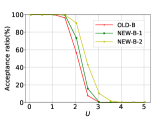
(a) Accept. ratio with changing $U$

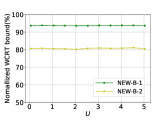
(b) Norm. bound with changing $U$

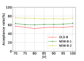
(c) Accept. ratio with changing $|V|$

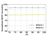
(d) Norm. bound with changing $|V|$

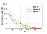
(e) Accept. ratio with changing $pr$

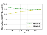
(f) Norm. bound with changing $pr$

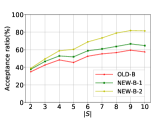
(g) Accept. ratio with changing $|S|$

(h) Norm. bound with changing $|S|$

Figure 5: Comparison of analysis precision of different bounds.

In this section, we experimentally evaluate the performance of our proposed analysis methods in terms of both precision and efficiency. We compare the following WCRT bounds in the experiments:

• OLD-B: the baseline bound in [18] (i.e., Theorem 2.1).

• NEW-B-1: our first new bound in Theorem 3.1.

• NEW-B-2: our second new bound in Theorem 4.1.

We assume the typed DAG tasks are periodic with a period $100$ with implicit deadlines (thus we evaluate not only the WCRT bound but also the schedulability of each task). We first define a default parameter setting, and then tune different parameters to evaluate the performance of the methods regarding different parameter changing trends. The default parameter setting is defined as follows:

• The number of types $|S|$ is randomly chosen in the range $[5,10]$, and the number of cores $M_{s}$ of each type $s$ is randomly chosen in $[2,11]$.

• The DAG structure of the task is generated by the method proposed in [9], where the number of vertices $|V|$ is randomly chosen in the range $[70,100]$ and the parallelism factor $p_{r}$ is randomly chosen in $[0.08,0.1]$ (the larger $p_{r}$, the more sequential is the graph).

• The total utilization $U$ of the typed DAG task is randomly chosen in $[1,3]$, and thus the total WCET of the task $vol(G)=U\times 100$.

• We use the Unnifast method [7] to distribute the total WCET to each individual vertex.

• Each vertex is randomly assigned a type in $S$.

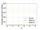
(a) Analysis time with changing $U$

(b) Analysis time with changing $pr$

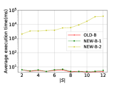
(c) Analysis time with changing $|S|$

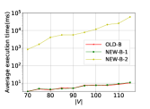
(d) Analysis time with changing $|V|$

Figure 6: Comparison of analysis efficiency of different bounds.

Figure 5 show the evaluation results for analysis precision with different parameters changed based on the default setting. Figure 5(a) and 5(b) show experiment results with changing $U$ (other parameters are the same as the default setting). Each point in Figure 5(a) represents the acceptance ratio of a WCRT bound, which is defined as the ratio between the number of tasks decided to be schedulable by a particular WCRT bound and the total number of tasks generated, with the target utilization $U$ on the axis. Figure 5(b) shows the normalized WCRT bound by our new methods (the baseline bound is $100\%$). Figure 5(c) and 5(d) are results with changing $|V|$, Figure 5(e) and 5(f) are results with changing $pr$, Figure 5(g) and 5(h) are results with changing $|S|$. From these experiments we can see that our proposed new bounds NEW-B-1 and NEW-B-2 consistently outperform OLD-B under various parameter settings.

Figure 6 evaluates the computational efficiency of different bounds, with different parameter changed based on the default setting (the same as Figure 5). Experiments results show that our first new bound NEW-B-1 is almost as efficient as OLD-B, while the computation procedure of NEW-B-2 takes much longer time. The lower efficiency of NEW-B-2 is due to the inherent hardness of its computation problem: exponential with respect to $|S|$ and high-order polynomial with respect to $|V|$ when $|S|$ is large. The computation time of NEW-B-2 first increases then decreases as $pr$ increases because the number of possible paths is relatively smaller with very small $pr$ (with which the paths are typically very short) and with large $pr$ (with which the task graphs are more sequential and thus the number of possible paths is not very large). The number of different core types in realistic heterogeneous multi-cores is usually a very small number. From Figure 6(c) we can see that the analysis procedure can finish in several seconds when the number of types is smaller than $8$, which should be acceptable for most offline design scenarios.

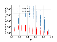
Figure 7: State space reduction by our computation algorithm for NEW-B-2.

Figure 7 shows the effectiveness of our proposed algorithm for computing NEW-B-2 based on the abstract path representation, by comparing the total number of tuples generated by our algorithm and the total number of paths of the task graph. We can see that using our abstraction the searching state space is reduced by typically $3$ to $4$ orders of magnitude.

6 Related Work

The most relevant related work is [18], which developed the baseline WCRT bound OLD-B as stated in Section 2.3. The analysis techniques of OLD-B are based on the classical work by Graham [13, 14] for untyped DAG (the special case of the model considered in this paper with only one type). The real-time scheduling problem for multiple recurring untyped DAG has been intensively studied, with different scheduling paradigm including federated scheduling [8, 2, 32] and global scheduling [29, 3, 5, 4, 30], which are also based on the classical work by Graham [13, 14]. Similarly, although we assume a single typed DAG task in this paper, our work would be a necessary step towards the scheduling and analysis of multiple recurring typed DAG tasks.

Yang et al. [40] studied the scheduling of multiple typed DAG tasks by decomposing each DAG task into a set of independent tasks with artificial release time and deadlines, and then analyzed these decomposed independent tasks by known methods under non-preemptive G-EDF (global earliest deadline first). The work in [40] is not directly comparable with our work due to the difference in problem models. However, when our method (based on Graham’s analysis framework) is extended to the multiple-DAG setting in the future, a comparison between these two families of techniques would be meaningful.

Yang et al. [40] studied the scheduling of multiple typed DAG tasks by decomposing each DAG task into a set of independent tasks with artificial release time and deadlines, and then analyzed these decomposed independent tasks by known methods under non-preemptive G-EDF (global earliest deadline first). The work in [40] is also applicable to the problem studies of this paper which is a special case of the multiple DAG setting in [40]. However, we did not include experimental comparison results between our method and [40] as the WCRT bounds yielded by the method in [40] is much larger than our method. The transformation to independent tasks in [40] is to handle the difficulty caused by multiple DAGs. Therefore, the comparison between our method and [40] under the single DAG setting will be unfairly in favor to us. We do not want to take of advantage of this to exaggerate the superiority of our method When our method (based on Graham s analysis framework) is extended to the multiple-DAG setting in the future, a comparison between these two families of techniques would be meaningful.

The scheduling problems with different workload-processor binding restrictions have been studied in the past, including the inclusive processing set restriction [27, 26, 16, 31] where for any two processor sets assigned to two tasks, one set must be the subset of the other, the interval processing set restriction [21, 22] where any two processing sets may have the same machines as the other but one is not a subset of the other and the tree-hierarchical processing set restrictions [17, 12] where each machine is described as a vertex of a tree and a processing set is a path from root to a leaf. These models are all different from our work. On the other hand, much work has been done on scheduling of independent tasks on heterogeneous multiprocessor with workload-processor binding restrictions [17, 23, 39], and [24, 25] provided comprehensive surveys for this line of work.

[20, 15] studied a special case of the problem model of this paper, which assumes (1) two types of machines, (2) chain-type precedence constraints (3) unit execution time for each scheduling unit. [19] studied the special case where the task graph structures are either in-trees, out-trees or disjoint unions of chains. [28] considered a special case with only two types of machines and assume the execution time of each scheduling unit to be constant so that they can generate a static scheduling list offline (which suffers timing anomalies if applied to the problem model in this paper where each task may execute shorter than its WCET).

7 Conclusion

This paper derives WCRT bounds for typed DAG parallel tasks on heterogeneous multi-cores, where the workload of each vertex in the DAG is bound to execute on a particular type of cores. The only known WCRT bound for this problem is grossly pessimistic and suffers the non-self-sustainability problem (a successful design may degrade to be unsuccessful when the parameters become better). We propose two new WCRT bounds to address these problems. The first new bound is more precise without increasing the time complexity and solves the non-self-sustainability problem. The second new bound explores more detailed task graph structure information to greatly improve the precision, but is computationally more expensive. We prove the strong NP-hardness of the computation problem for the second bound, and develop an efficient algorithm which has polynomial time complexity if the number of types is a constant. In next step we will extend the results of this paper to the general setting of multiple recurring typed DAG tasks and compare it with our families of techniques such as the decomposition based approach [40]. Another possible direction for our future work is to develop more efficient algorithms that compute NEW-B-2 approximately, which hopefully can give bounds reasonably close to those computed by the algorithm of this paper in much shorter time.

Meiling Han as born in Liaocheng, Shandong of China in 1988. She received her master’s degree in computer applications technology from Shenyang Agricultural University, China in 2013, she is a Ph.D. candidate at the School of Computer Science and Engineering of Northeastern University, China. Her research interests are broadly in embedded real-time systems, especially the real-time scheduling on multiprocessor systems.

Nan Guan is currently an assistant professor at the Department of Computing, The Hong Kong Polytechnic University. Dr Guan received his BE and MS from Northeastern University, China in 2003 and 2006 respectively, and a PhD from Uppsala University, Sweden in 2013. Before joining PolyU in 2015, he worked as a faculty member in Northeastern University, China. His research interests include real-time embedded systems and cyber-physical systems. He received the EDAA Outstanding Dissertation Award in 2014, the Best Paper Award of IEEE Real-time Systems Symposium (RTSS) in 2009, the Best Paper Award of Conference on Design Automation and Test in Europe (DATE) in 2013.

Jinghao Sun received the MS and PhD degree in computer science from Dalian University of Technology in 2012. He is an associated professor at Northeastern University, China. He was a postdoctoral fellow in the Department of Computing at Hong Kong Polytechnic University between 2016 to 2017, working on scheduling algorithms for multi-core real time systems. His research interests include algorithms, schedulability analysis and optimization methods.

Qingqiang He received the BS degree in computer science and technology from Northeastern University, China, in 2014, and the MS degree in computer software and theory from Northeastern University, China, in 2017. Now he is working as a research assistant in Hong Kong Polytechnic University. His research interests include embedded real-time system, real-time scheduling theory, and distributed leger.

Qingxu Deng received his Ph.D. degree in computer science from Northeastern University, China, in 1997. He is a professor of the School of Computer Science and Engineering , Northeastern University, China, where he serves as the Director of institute of Cyber Physical Systems. His main research interests include Cyber-Physical systems, embedded systems, and real-time systems.

Weichen Liu Weichen Liu (S’07-M’11) is an assistant professor at School of Computer Science and Engineering, Nanyang Technological University, Singapore. He received the PhD degree from the Hong Kong University of Science and Technology, Hong Kong, and the BEng and MEng degrees from Harbin Institute of Technology, China. Dr. Liu has authored and co-authored more than 70 publications in peer-reviewed journals, conferences and books, and received the best paper candidate awards from ASP-DAC 2016, CASES 2015, CODES+ISSS 2009, the best poster awards from RTCSA 2017, AMD-TFE 2010, and the most popular poster award from ASP-DAC 2017. His research interests include embedded and real-time systems, multiprocessor systems and network-on-chip.

References

- [1] Theodore P. Baker and Sanjoy K. Baruah. Sustainable multiprocessor scheduling of sporadic task systems. In 21st Euromicro Conference on Real-Time Systems, ECRTS 2009, Dublin, Ireland, July 1-3, 2009, pages 141–150. IEEE Computer Society, 2009.
- [2] Sanjoy Baruah. Improved multiprocessor global schedulability analysis of sporadic DAG task systems. In 26th Euromicro Conference on Real-Time Systems, ECRTS 2014, Madrid, Spain, July 8-11, 2014, pages 97–105. IEEE Computer Society, 2014.
- [3] Sanjoy Baruah. The federated scheduling of constrained-deadline sporadic DAG task systems. In Wolfgang Nebel and David Atienza, editors, Proceedings of the 2015 Design, Automation & Test in Europe Conference & Exhibition, DATE 2015, Grenoble, France, March 9-13, 2015, pages 1323–1328. ACM, 2015.
- [4] Sanjoy Baruah. Federated scheduling of sporadic DAG task systems. In 2015 IEEE International Parallel and Distributed Processing Symposium, IPDPS 2015, Hyderabad, India, May 25-29, 2015, pages 179–186. IEEE Computer Society, 2015.
- [5] Sanjoy Baruah. The federated scheduling of systems of conditional sporadic DAG tasks. In Alain Girault and Nan Guan, editors, 2015 International Conference on Embedded Software, EMSOFT 2015, Amsterdam, Netherlands, October 4-9, 2015, pages 1–10. IEEE, 2015.
- [6] Matthias Beckert and Rolf Ernst. Response time analysis for sporadic server based budget scheduling in real time virtualization environments. ACM Trans. Embedded Comput. Syst., 16(5):161:1–161:19, 2017.
- [7] Enrico Bini and Giorgio C. Buttazzo. Measuring the performance of schedulability tests. Real-Time Systems, 30(1-2):129–154, 2005.
- [8] Vincenzo Bonifaci, Alberto Marchetti-Spaccamela, Sebastian Stiller, and Andreas Wiese. Feasibility analysis in the sporadic DAG task model. In 25th Euromicro Conference on Real-Time Systems, ECRTS 2013, Paris, France, July 9-12, 2013, pages 225–233. IEEE Computer Society, 2013.
- [9] Daniel Cordeiro, Grégory Mounié, Swann Perarnau, Denis Trystram, Jean-Marc Vincent, and Frédéric Wagner. Random graph generation for scheduling simulations. In L. Felipe Perrone, Giovanni Stea, Jason Liu, Adelinde M. Uhrmacher, and Manuel Villén-Altamirano, editors, 3rd International Conference on Simulation Tools and Techniques, SIMUTools ’10, Malaga, Spain - March 16 - 18, 2010, page 60. ICST/ACM, 2010.
- [10] NVIDA CUDA[onlie]. https://developer.nvidia.com/cuda-zone.
- [11] Sanjoy Dasgupta, Christos H Papadimitriou, and Umesh Vazirani. Algorithms. McGraw-Hill, Inc., 2006.
- [12] Leah Epstein and Asaf Levin. Scheduling with processing set restrictions: Ptas results for several variants. 133:586–595, 2011.
- [13] R. L. Graham. Bounds for certain multiprocessing anomalies. 45:1563–1581, 1966.
- [14] R. L. Graham. Bounds on multiprocessing timing anomalies. SIAM Journal on Applied Mathematics, 17:416–429, 1969.
- [15] Jiye Han, Jianjun Wen, and Guochuan Zhang. A new approximation algorithm for uet-scheduling with chain-type precedence constraints. Computers & OR, 25(9):767–771, 1998.
- [16] Zhao hong Jia, Kai Li, and Joseph Y.-T. Leung. Effective heuristic for makespan minimization in parallel batch machines with non-identical capacities. 169:1–10, 2015.
- [17] Yumei Huo and Joseph Y.-T. Leung. Fast approximation algorithms for job scheduling with processing set restrictions. 411:3947–3955, 2010.
- [18] Jeffrey M. Jaffe. Bounds on the scheduling of typed task systems. SIAM Journal on Computing, 9(3):541–551, 1980.
- [19] Klaus Jansen. Analysis of scheduling problems with typed task systems. Discrete Applied Mathematics, 52(3):223–232, 1994.
- [20] Klaus Jansen, Gerhard J. Woeginger, and Zhongliang Yu. Uet-scheduling with chain-type precedence constraints. Computers & OR, 22(9):915–920, 1995.
- [21] Shlomo Karhi and Dvir Shabtay. On the optimality of the tls algorithm for solving the online-list scheduling problem with two job types on a set of multipurpose machines. 26:198–222, 2013.
- [22] Shlomo Karhi and Dvir Shabtay. Online scheduling of two job types on a set of multipurpose machines. 150:155–162, 2014.
- [23] Kangbok Lee, Joseph Y.-T. Leung, and Michael L. Pinedo. Scheduling jobs with equal processing times subject to machine eligibility constraints. 14:27–38, 2011.
- [24] Joseph Y.-T. Leung and Chung-Lun Li. Scheduling with processing set restrictions: A survey. 116:251–262, 2008.
- [25] Joseph Y.-T. Leung and Chung-Lun Li. Scheduling with processing set restrictions: A literature update. 175:1–11, 2016.
- [26] Chung-Lun Li and Kangbok Lee. A note on scheduling jobs with equal processing times and inclusive processing set restrictions. JORS, 67(1):83–86, 2016.
- [27] Chung-Lun Li and Qingying Li. Scheduling jobs with release dates, equal processing times, and inclusive processing set restrictions. JORS, 66(3):516–523, 2015.
- [28] Dingchao Li and N. Ishii. Scheduling task graphs onto heterogeneous multiprocessors.
- [29] Jing Li, Jian-Jia Chen, Kunal Agrawal, Chenyang Lu, Christopher D. Gill, and Abusayeed Saifullah. Analysis of federated and global scheduling for parallel real-time tasks. In 26th Euromicro Conference on Real-Time Systems, ECRTS 2014, Madrid, Spain, July 8-11, 2014, pages 85–96. IEEE Computer Society, 2014.
- [30] Jing Li, David Ferry, Shaurya Ahuja, Kunal Agrawal, Christopher D. Gill, and Chenyang Lu. Mixed-criticality federated scheduling for parallel real-time tasks. Real-Time Systems, 53(5):760–811, 2017.
- [31] Shuguang Li. Parallel batch scheduling with inclusive processing set restrictions and non-identical capacities to minimize makespan. European Journal of Operational Research, 260(1):12–20, 2017.
- [32] Alessandra Melani, Marko Bertogna, Vincenzo Bonifaci, Alberto Marchetti-Spaccamela, and Giorgio C. Buttazzo. Response-time analysis of conditional DAG tasks in multiprocessor systems. In 27th Euromicro Conference on Real-Time Systems, ECRTS 2015, Lund, Sweden, July 8-10, 2015, pages 211–221. IEEE Computer Society, 2015.
- [33] OMAP[online]. https://en.wikipedia.org/wiki/OMAP.
- [34] Openmp [online]. Openmp application program interface version 4.5. https://www.openmp.org/.
- [35] OpenCL[online]. https://www.khronos.org/opencl/.
- [36] Tegra Processors[online]. https://www.nvidia.com/object/tegra.html.
- [37] Zynq-7000 SoC[online]. https://www.xilinx.com/products/silicon-devices/soc/zynq-7000.html.
- [38] Ashish Venkat and Dean M. Tullsen. Harnessing ISA diversity: Design of a heterogeneous-isa chip multiprocessor. In ACM/IEEE 41st International Symposium on Computer Architecture, ISCA 2014, Minneapolis, MN, USA, June 14-18, 2014, pages 121–132. IEEE Computer Society, 2014.
- [39] Jia Xu and Zhaohui Liu. Online scheduling with equal processing times and machine eligibility constraints. 572:58–65, 2015.
- [40] Kecheng Yang, Ming Yang, and James H. Anderson. Reducing response-time bounds for dag-based task systems on heterogeneous multicore platforms. In Alain Plantec, Frank Singhoff, Sébastien Faucou, and Luís Miguel Pinho, editors, Proceedings of the 24th International Conference on Real-Time Networks and Systems, RTNS 2016, Brest, France, October 19-21, 2016, pages 349–358. ACM, 2016.