Abstract: Within the framework of Becchi–Rouet–Stora–Tyutin (BRST) formalism, we show that the four $(3+1)$-dimensional (4D) massive Abelian 2-form gauge theory (without any interaction with matter fields) is a model for the Hodge theory because its discrete and continuous symmetry transformations (and their corresponding Noether conserved charges) provide the physical realizations of the de Rham cohomological operators of differential geometry at the algebraic level. For this purpose, we incorporate the pseudo-scalar and axial-vector fields which appear in the theory with negative kinetic terms (but with proper definition of mass). The negative kinetic terms, for the above fields, are essential so that our theory could respect the discrete symmetry transformations which provide the physical realizations of the Hodge duality operation in the domain of differential geometry. Thus, our present endeavour, not only provides the physical realizations of all the mathematical ingredients connected with the de Rham cohomological operators of differential geometry, it also sheds light on the existence and emergence of fields with negative kinetic terms. We discuss the implications and relevance of the latter fields in the context of current models of dark matter and dark energy as well as the bouncing models of Universe.

PACS numbers: 11.15.-q; 11.30.-j; 03.70.+k; 95.35.+d

Keywords: 4D massive Abelian 2-form gauge theory; Nilpotent symmetries; Bosonic symmetry; Massive model of Hodge theory; Fields with negative kinetic term; Cosmological models of Universe

1 Introduction

The standard model of particle physics, based on the fundamental principles of local gauge invariant (non-)Abelian 1-form gauge theories, is one of the most successful theories of high energy physics where there is a stunning degree of agreement between theory and experiment. This model also provides the theoretical framework for the unification of electromagnetic, weak and strong interactions of nature. However, one has to go beyond the purview of standard model of particle physics in view of the fact that the neutrinos have been found to be massive by precise experimental observations. This experimental result is one of the many crucial reasons that has compelled theoretical physicists to propose $new$ models in high energy physics that are mostly based on the ideas of supersymmetry (e.g. supersymmetric models of quantum field theories and superstring theories). One of the hottest candidates, in this direction, is the basic ideas behind (super)string theories which lead to the theoretical description of quantum gravity. These theories also provide a theoretical framework for the unification of all four fundamental forces of nature. In the quantum excitations of the superstring theories, the higher $p$-form ($p=2,3,4,...$) gauge fields appear very naturally thereby going beyond the realm of standard model of particle physics in a subtle manner (because the latter theoretical model, as stated earlier, is based only on the basic principles of local gauge invariant (non-)Abelian 1-form theories). Thus, the study of higher $p$-form ($p=2,3,4,...$) gauge theories has become quite interesting and important during the last few years due to its connection with the (super)strings and their quantum excitations.

In the covariant canonical quantization of gauge and reparametrization invariant theories of any kind, the role of Becchi–Rouet–Stora–Tyutin (BRST) formalism [1, 2, 3, 4] is quite crucial as it maintains unitarity and “quantum” gauge (i.e. BRST) invariance at any arbitrary order of perturbative computations for any physically allowed process. We have established, in our earlier works (see, e.g. for a brief review [5, 6]), that any arbitrary Abelian $p$-form ($p=1,2,3,...$) gauge theory, in $\text{D}=2p$ dimensions of spacetime, is endowed with the (anti-)BRST as well as (anti-)co-BRST symmetries within the framework of BRST formalism. Such theories have been shown to provide a set of tractable physical examples for the Hodge theory where the symmetries (and corresponding conserved charges) provide the physical realizations of the de Rham cohomological operators of differential geometry [7, 8, 9, 10]. In our earlier works (see, e.g. [5, 6, 11, 12, 13, 14, 15, 16]), we have established that the 2D (non-)Abelian 1-form gauge theories, 4D Abelian 2-form and 6D Abelian 3-form gauge theories provide the examples of Hodge theory. Such studies are physically important because we have shown that the 2D (non-)Abelian 1-form gauge theories provide a set of new models of topological field theories (TFTs) [17] which capture a few aspects of Witten-type TFTs [18] and some salient features of Schwarz-type TFTs [19]. In addition, it has been shown that the free 4D Abelian 2-form and 6D Abelian 3-form gauge theories are the examples of quasi-TFTs [20, 6]. An interacting Abelian 1-form gauge theory (with $massless$ Dirac fields) has also been shown to be a perfect model of Hodge theory [21] because of its various discrete and continuous symmetries and their connections with the algebra of de Rham cohomological operators of differential geometry (including the Hodge duality operation).

All the theories, that have been mentioned in the previous paragraph, are massless Abelian $p$-form gauge theories which have been shown to be the models for the Hodge theory in $\text{D}=2p$ dimensions of spacetime (within the framework of BRST formalism [5, 6]). In our earlier work [22], for the first time, we have demonstrated that the Stückelberg modified 2D Proca theory (i.e. a massive 2D Abelian 1-form gauge theory) is also a model for the Hodge theory provided we invoke a new field in the theory (which is nothing but a pseudo-scalar field that turns up in the theory with a negative kinetic term). The continuous and discrete symmetries of the theory enforce the scalar field of the theory to possess the positive kinetic term but the pseudo-scalar field of the theory, as pointed out earlier, is forced to acquire a negative kinetic term (with a properly well-defined mass). Hence, the latter field mimics one of the key properties of the dark matter which is quite popular in modern literature [23, 24, 25, 26]. Thus, the 2D Stückelberg modified Proca theory (i.e. a massive 2D Abelian 1-form gauge theory) provides a theoretical basis and motivation to look for the discussion of existence and emergence of fields with negative kinetic terms in the physical four $(3+1)$-dimensional (4D) theories within the framework of quantum field theory (QFT) where the BRST formalism plays a crucial role (as far as the symmetry properties and their conserved charges are concerned).

The central theme of our present investigation is to carry forward the ideas [22] of 2D Stückelberg modified massive Abelian 1-form gauge theory (i.e. the modified Proca theory) to the four $(3+1)$-dimensional massive Abelian 2-form gauge theory and demonstrate the existence of axial-vector and pseudo-scalar fields which turn up with negative kinetic terms (but with well-defined mass as they satisfy the Klein–Gordon equation). In fact, the symmetries of the Stückelberg modified massive 4D Abelian 2-form gauge theory are such that they fix all the signatures of all the terms that appear in the coupled (but equivalent) Lagrangian densities. These symmetries are responsible for the proof of this massive physical 4D model to become an example of Hodge theory within the framework of BRST formalism. To be precise, we have six continuous symmetries in the theory, out of which, four are fermionic (supersymmetric-type) and two of them are bosonic in nature. We have shown that the algebra of continuous symmetry transformation operators (and corresponding conserved charges) obey exactly the same algebra as the algebra of de Rham cohomological operators of differential geometry. In addition to the above six continuous symmetries, we have also shown the existence of two appropriate discrete symmetries in the theory which provide the physical realizations of the Hodge duality operation of differential geometry at the algebraic level in the well-known relationship between the co-exterior derivative and exterior derivative. As far as the physical consequences of our present study is concerned, we observe that the emergence of the fields/particles with the negative kinetic terms as one of the possible candidates of dark matter/dark energy. This result is the culmination of all our earlier works [5, 6, 11, 12, 13, 14, 15, 16] where we have proposed the existence of 4D and 6D quasi-TFTs and a couple of $new$ models for the 2D TFTs within the framework of BRST formalism (see, e.g. [5, 6, 11, 12, 13, 14, 15, 16, 17] for details).

Against the backdrop of our discussions in the previous paragraphs, we would like to say a few things about one of the the modern theoretical understandings of the possible candidates for the dark matter and dark energy [23, 24, 25, 26]. The pressing problems of theoretical physics of modern times is to explain the accelerated expansion of our Universe which has been established by several experimental observations [27, 28, 29, 30, 31, 32]. The idea of the existence of dark energy has been invoked to explain the accelerated expansion (of our present Universe). During the past few years, the fields/particles with negative kinetic terms have been considered by many theoretical and experimental researchers as the one of the possible candidates for the dark matter and dark energy [33, 34, 35, 36, 37]. One of the central outcomes of our present investigation is to demonstrate the existence of a massive pseudo-scalar and an axial-vector fields in the discussions of the massive 4D Abelian 2-form gauge theory where the above fields (with negative kinetic terms) appear due to the symmetry considerations alone. In fact, in our earlier works on 2D Proca theory [22], we have established the existence of a massive pseudo-scalar field with negative kinetic term (see, also Appendix A) which is required in the proof of this theory to be a model for the Hodge theory. It is but natural to conclude that, in the massless limit, the above pseudo-scalar field becomes a possible candidate for the dark energy. Thus, in our present endeavour, we provide the unified theoretical explanation for the possible existence and emergence of the fields corresponding to the dark matter and dark energy within the framework of QFT where the BRST formalism plays a decisive role.

The following motivating factors have been at the heart of our present investigation. First and foremost, so far, we have been able to prove the 2D Proca (i.e. a massive Abelian 1-form) theory to be an example of Hodge theory [22]. Thus, it has been a challenging problem for us to prove a massive physical 4D Abelian 2-form theory to be a model for the Hodge theory. We have accomplished this goal in our present endeavour. Second, in our earlier work [15], we have shown that the 4D free Abelian 2-form gauge theory is a model for the Hodge theory. Thus, it has been a tempting and interesting problem for us to prove the massive version of the above 4D theory to be a model for the Hodge theory, too. We have achieved this objective in our present investigation. Finally, the underlying mathematical/theoretical exercises (connected with the proof of the models to be the examples of Hodge theory) have been done by us for the 1D, 2D, 4D and 6D theories which are nothing but the toy models in 1D [38, 39] as well as the field theoretical systems [2, 13, 14, 15, 16, 17, 20, 21, 22] in various other dimensions. It has been a challenge for us to show the physical implications of these studies. In our present investigation, we have demonstrated that such studies lead to the emergence of fields/particles with negative kinetic terms which might be, perhaps, one of the possible candidates for the dark matter and dark energy [23, 24, 25, 26] within the framework of BRST formalism.

The contents of our present investigation are organized as follows. First of all, we discuss the bare essentials of the Stückelberg approach to convert the massive 4D Abelian 2-form theory (endowed with second-class constraints) into a gauge theory (endowed with first-class constraints) by adding some extra fields (i.e. the analogue of the usual Stückelberg’s field) in Section 2. The linearized version of the coupled (but equivalent) Lagrangian densities (that respect the (anti-)BRST symmetry transformations together) are discussed in Section 3. Our Section 4 deals with the discussions on the off-shell nilpotent (anti-)co-BRST symmetry transformations. In Section 5, we elaborate on the existence of a unique bosonic symmetry transformation for our (anti-)BRST and (anti-)co-BRST symmetry invariant Lagrangian densities. In Section 6, we discuss the existence of the ghost-scale symmetry and discrete symmetry transformations. Our Section 7 deals with the algebraic structures of all the continuous symmetry transformations (and corresponding conserved Noether charges) where we establish their connection with the algebra of the de Rham cohomological operators. In Section 8, we concisely comment on the fields with $negative$ kinetic terms which are the possible candidates for the dark matter/dark energy. Finally, we make some concluding remarks in Section 9 and point out a few future directions for further investigation(s). In this section, we also mention the physical implications of the fields with negative kinetic term in the context of cosmological models.

In our Appendix A, we briefly mention the ideas behind the existence of a pseudo-scalar field with negative kinetic term in the context of a 2D Proca theory (which is a precursor to our discussions on our present 4D massive Abelian 2-form theory). Our Appendix B is devoted to the discussion of change in the kinetic term ($\frac{1}{12}\,H^{\mu\nu\eta}H_{\mu\nu\eta}$) for the gauge field $B_{\mu\nu}$ due to the redefinition of the gauge field $B_{\mu\nu}$ (cf. Eq. (2) below). In our Appendix C, we demonstrate diagrammatically the existence of the CF-type restrictions for our model of a 4D Stückelberg modified massive gauge theory .

Convention and notations:

We adopt the convention of the left-derivative w.r.t. all the fermionic fields of our theory in appropriate/relevant computations. The background flat metric tensor for the 4D Minkowskian spacetime manifold is chosen to be: $\eta_{\mu\nu}\equiv\eta^{\mu\nu}$ = diag $(+1,-1,-1,-1)$ so that for a non-null vector $A_{\mu}$, the dot product $\partial\cdot A=\eta^{\mu\nu}\partial_{\mu}A_{\nu}=\partial_{0}A_{0}-\partial_{i}A_{i}\equiv\eta_{\mu\nu}\partial^{\mu}A^{\nu}$ where the Greek indices $\mu,\nu,\lambda,...=0,1,2,3$ correspond to the time and space directions and the Latin indices $i,j,k,...=1,2,3$ stand for the space directions only. We choose the 4D Levi-Civita tensor $\varepsilon_{\mu\nu\lambda\kappa}$ such that $\varepsilon_{0123}=+1=-\varepsilon^{0123}$ and $\varepsilon_{\mu\nu\lambda\kappa}\varepsilon^{\mu\nu\lambda\kappa}=-\,4!$, $\varepsilon_{\mu\nu\lambda\kappa}\varepsilon^{\mu\nu\lambda\rho}=-\,3!\,\delta^{\rho}_{\kappa}$, etc., and $\varepsilon_{0ijk}=-\varepsilon^{0ijk}\equiv\epsilon_{ijk}$ is the 3D Levi-Civita tensor. We adopt the notations $s_{(a)b}$ and $s_{(a)d}$ for the nilpotent (anti-)BRST and (anti-)co-BRST [i.e (anti-)dual BRST] transformations (and corresponding charges are denoted by $Q_{(a)b}$ and $Q_{(a)d}$) in the whole body of our text. These transformations (i.e. $s_{(a)b}$ and $s_{(a)d}$) are supersymmetric-type in nature as they transform bosonic fields into fermionic fields and vic̀e-versa. We also choose the convention of derivative w.r.t. the second-rank antisymmetric tensor field as: $(\partial B_{\mu\nu}/\partial B_{\rho\sigma})=\frac{1}{2!}\,\big{(}\delta^{\rho}_{\mu}\,\delta^{\sigma}_{\nu}-\delta^{\rho}_{\nu}\,\delta^{\sigma}_{\mu}\big{)}$, etc.

Standard definitions:

We briefly mention here the basic concepts behind the key definitions of a few aspects of differential geometry that are needed for the full appreciation of our present work:

1. de Rham cohomological operators: On a compact manifold without a boundary, we define a set of three operators ($d$, $\delta$, $\Delta$) which are christened as the exterior derivative operator, co-exterior derivative operator and Laplacian operator, respectively. These operators follow an algebra: $d^{2}=0$, $\delta^{2}=0$, $\Delta=\{d,\delta\}$, $[\Delta,d]=[\Delta,\delta]=0$ which is popularly known as the Hodge algebra where the (co-)exterior derivatives $(\delta)d$ are connected by the relationship: $\delta=\pm\,*\,d\,*$. Here $*$ is nothing but the Hodge duality operation (on a given compact manifold without a boundary).

2. Hodge decomposition theorem: On the manifold discussed above, any arbitrary form $f_{n}$ (of degree $n$) can be uniquely written as the sum of a harmonic form $(\omega_{n})$, an exact form $(e_{n})$ and a co-exact form $(c_{n})$ as

   $$f_{n}=\omega_{n}+e_{n}+c_{n},$$

   where $e_{n}=dg_{n-1}$, $c_{n}=\delta h_{n+1}$. Here $g_{n-1}$ and $h_{n+1}$ are the non-zero forms of degree $(n-1)$ and $(n+1)$, respectively. In other words, we have the following

   $$f_{n}=\omega_{n}+d\;g_{n-1}+\delta\;h_{n+1},$$

   where $\omega_{n}$ is the harmonic form (i.e. $\Delta\omega_{n}=0\Rightarrow d\omega_{n}=0$ and $\delta\omega_{n}=0$).

2 Preliminaries: Lagrangian formulation

We begin with the four $(3+1)$-dimensional (4D) Kalb–Ramond Lagrangian density [40, 41, 42] for the free Abelian 2-form massive theory (with rest mass $m$) as (see, e.g. [43] for details)

$${\cal L}_{(0)}=\frac{1}{12}\,H^{\mu\nu\eta}H_{\mu\nu\eta}-\frac{m^{2}}{4}\,B^{\mu\nu}B_{\mu\nu},$$ (1)

where the antisymmetric $(B_{\mu\nu}=-B_{\nu\mu})$ tensor field $B_{\mu\nu}$ is the 4D Abelian 2-form $\big{(}B^{(2)}=\frac{1}{2!}\,(dx^{\mu}\wedge dx^{\nu})\,B_{\mu\nu}\big{)}$ gauge field and the curvature (i.e. field strength) tensor $H_{\mu\nu\eta}=\partial_{\mu}B_{\nu\eta}+\partial_{\nu}B_{\eta\mu}+\partial_{\eta}B_{\mu\nu}$ is derived from the 3-form $\big{(}H^{(3)}=dB^{(2)}\equiv\frac{1}{3!}\,(dx^{\mu}\wedge dx^{\nu}\wedge dx^{\eta})\,H_{\mu\nu\eta}\big{)}$. It is clear that the mass dimension of $B_{\mu\nu}$ is $[M]$ in the natural units ($\hbar=c=1$) for the 4D theory. Because of the presence of mass term $(-\frac{m^{2}}{4}\,B_{\mu\nu}\,B^{\mu\nu})$, there is no gauge invariance at this stage because the above Lagrangian density is endowed with the second-class constraints (see, e.g. [43]) in the terminology of Dirac’s prescription for the classification scheme [44, 45]. We note that the Euler-Lagrange equation of motion (EL-EOM) from ${\cal L}_{(0)}$ is: $\partial_{\mu}H^{\mu\nu\eta}+m^{2}\,B^{\nu\eta}=0$. It is clear that we obtain the usual Klein–Gordan equation [i.e. $(\Box+m^{2})\,B_{\mu\nu}=0$] for the massive Abelian 2-form field $(B_{\mu\nu})$ because we note that the EL-EOM: $\partial_{\mu}H^{\mu\nu\eta}+m^{2}\,B^{\nu\eta}=0$ implies that $\partial_{\mu}B^{\mu\nu}=\partial_{\nu}B^{\mu\nu}=0$. The latter conditions are true (i.e. $\partial_{\nu}\partial_{\mu}H^{\mu\nu\eta}+m^{2}\,\partial_{\nu}B^{\nu\eta}=0\Rightarrow\partial_{\nu}B^{\nu\eta}=0$) because, for the massive Abelian 2-form theory, we note that the rest mass $m\neq 0$.

Using the Stückelberg’s technique, it can be checked that, we can have the following modification/redefinition for the antisymmetric tensor field $B_{\mu\nu}$

$$B_{\mu\nu} \to B_{\mu\nu}-\frac{1}{m}\,\Phi_{\mu\nu}-\frac{1}{2\,m}\,\varepsilon_{\mu\nu\eta\kappa}\,\tilde{\Phi}^{\eta\kappa}$$ (2)

$$\equiv B_{\mu\nu}-\frac{1}{m}\,\big{(}\partial_{\mu}\phi_{\nu}-\partial_{\nu}\phi_{\mu}+\varepsilon_{\mu\nu\eta\kappa}\,\partial^{\eta}\tilde{\phi}^{\kappa}\big{)}$$

$$\equiv B_{\mu\nu}-\frac{1}{m}\,\Phi_{\mu\nu}-\frac{1}{m}\,{\cal F}_{\mu\nu},$$

where the Abelian 2-form $\Phi^{(2)}=\frac{1}{2!}\,(dx^{\mu}\wedge dx^{\nu})\,\Phi_{\mu\nu}\equiv d\,\Phi^{(1)}$ (with vector 1-form $\Phi^{(1)}=dx^{\mu}\,\phi_{\mu}$, $\Phi_{\mu\nu}=\partial_{\mu}\phi_{\nu}-\partial_{\nu}\phi_{\mu}$) is constructed from a vector field $\phi_{\mu}$. On the contrary, the dual antisymmetric tensor $\tilde{\Phi}_{\mu\nu}=\partial_{\mu}\tilde{\phi}_{\nu}-\partial_{\nu}\tilde{\phi}_{\mu}$ is constructed with the help of an axial-vector $\tilde{\phi}_{\mu}$ which is derived from the axial-vector 1-form $\tilde{\Phi}^{(1)}=dx^{\mu}\,\tilde{\phi}_{\mu}$. To make the parity of $B_{\mu\nu}$, $\Phi_{\mu\nu}$ and $\tilde{\Phi}_{\mu\nu}$ on equal footing, we have taken, in Eq. (2), the following

$$*\,d\,\tilde{\Phi}^{(1)}=\frac{1}{2!}\,(dx^{\mu}\wedge dx^{\nu})\,{\cal F}_{\mu\nu},$$ (3)

where ${\cal F}_{\mu\nu}=\frac{1}{2!}\,\varepsilon_{\mu\nu\eta\kappa}\,\tilde{\Phi}^{\eta\kappa}$ and $*$ is the Hodge duality operation on a 2-form $(d\,\tilde{\Phi}^{(1)})$ which is defined on a flat 4D Minkowskian spacetime manifold. It is straightforward to check that the Lagrangian density (1) transforms to the following [43]

$${\cal L}_{(0)}\to{\cal L}_{(1)} = \frac{1}{12}\,H^{\mu\nu\eta}H_{\mu\nu\eta}-\frac{m^{2}}{4}\,B^{\mu\nu}B_{\mu\nu}-\frac{1}{4}\,\Phi^{\mu\nu}\Phi_{\mu\nu}$$ (4)

$$+ \frac{1}{4}\,\tilde{\Phi}^{\mu\nu}\tilde{\Phi}_{\mu\nu}+\frac{m}{2}\,B^{\mu\nu}\Phi_{\mu\nu}+\frac{m}{4}\,\varepsilon^{\mu\nu\eta\kappa}\,B_{\mu\nu}\tilde{\Phi}_{\eta\kappa},$$

(modulo some total spacetime derivative terms) under the modification (2). It should be noted that the kinetic term (i.e. $\frac{1}{12}\,H^{\mu\nu\eta}H_{\mu\nu\eta}$) does not change in a meaningful manner under the redefinition/modification (2). For our 4D theory, it is straightforward to note that the mass dimension of fields $\phi_{\mu}$ and $\tilde{\phi}_{\mu}$ is $[M]$ in the natural unit where $\hbar=c=1$. The above Lagrangian density respects (i.e. $\delta^{(1)}_{g}{\cal L}_{(1)}=0$) the following “scalar” gauge transformation $\delta_{g}^{(1)}$, namely;

$$\delta^{(1)}_{g}\phi_{\mu}=\partial_{\mu}\Sigma,\qquad\delta^{(1)}_{g}\tilde{\phi}_{\mu}=\partial_{\mu}\tilde{\Sigma},\qquad\delta^{(1)}_{g}B_{\mu\nu}=0,$$ (5)

where $\Sigma$ is a scalar and $\tilde{\Sigma}$ is a pseudo-scalar local gauge transformation parameters. In addition, it also respects the following other symmetry (i.e. “tensor” gauge symmetry) transformations

$$\delta^{(2)}_{g}\phi_{\mu}=-\,m\,\Lambda_{\mu},\qquad\delta^{(2)}_{g}\tilde{\phi}_{\mu}=0,\qquad\delta^{(2)}_{g}B_{\mu\nu}=-\,(\partial_{\mu}\Lambda_{\nu}-\partial_{\nu}\Lambda_{\mu}),$$ (6)

where $\Lambda_{\mu}$ is a local Lorentz vector gauge transformation parameter. To be more precise, it can be explicitly checked that $\delta^{(2)}_{g}{\cal L}_{(1)}=\partial_{\mu}\big{[}-m\,\varepsilon^{\mu\nu\eta\kappa}\,\Lambda_{\nu}\,(\partial_{\eta}\tilde{\phi}_{\kappa})\big{]}$. Thus, the action integral $S=\int d^{4}x\,{\cal L}_{(1)}$ remains invariant under $\delta^{(2)}_{g}$ for physically well-defined fields that vanish-off at $\pm\,\infty$. These “classical” continuous symmetry transformations (5) and (6) would play very important roles in our later discussions on the subject of off-shell nilpotent and absolutely anticommuting (anti-)BRST symmetries which are “quantum” in nature (cf. Section 3).

We shall focus on the form of the Lagrangian density ${\cal L}_{(1)}$ for our further discussions within the framework of BRST formalism where we shall discuss the (anti-)BRST and (anti-)co-BRST symmetry transformations (cf. Sections 3 and 4) which are basic ingredients to prove the present 4D massive Abelian 2-form gauge theory to be a field-theoretic model for the Hodge theory. We note that the Lagrangian density ${\cal L}_{(1)}$ is singular w.r.t. all the three basic fields ($B_{\mu\nu},\,\phi_{\mu},\tilde{\phi}_{\mu}$) of the theory (see, e.g. [44, 45]). Thus, for the BRST quantization of the theory, we have to add the gauge-fixing terms which have their origin in the co-exterior derivative $\delta=-*d*$ (where $*$ is the Hodge duality operator on the 4D flat Minkowskian spacetime manifold and minus sign has been taken because our background spacetime manifold is an even dimensional). It can be readily checked that we have the following:

$$\delta\,B^{(2)}=-*d*B^{(2)}=dx^{\mu}(\partial^{\nu}B_{\nu\mu}),$$

$$\delta\,\phi^{(1)}=-*d*\phi^{(1)}=(\partial^{\mu}\phi_{\mu})\equiv\big{(}\partial\cdot\phi\big{)},$$

$$\delta\,\tilde{\phi}^{(1)}=-*d*\tilde{\phi}^{(1)}=(\partial^{\mu}\tilde{\phi}_{\mu})\equiv\big{(}\partial\cdot\tilde{\phi}\big{)}.$$ (7)

Thus, the Lagrangian density ${\cal L}_{(1)}$ is modified and generalized to ${\cal L}_{(2)}$ as:

$${\cal L}_{(1)}\to{\cal L}_{(2)} = {\cal L}_{(1)}+\frac{1}{2}(\partial^{\nu}B_{\nu\mu})(\partial_{\rho}B^{\rho\mu})-\frac{1}{2}(\partial_{\mu}\phi^{\mu})(\partial_{\nu}\phi^{\nu})+\frac{1}{2}(\partial_{\mu}\tilde{\phi}^{\mu})(\partial_{\nu}\tilde{\phi}^{\nu})$$ (8)

$$\equiv {\cal L}_{(1)}+\frac{1}{2}\,(\partial^{\nu}B_{\nu\mu})^{2}-\frac{1}{2}\,(\partial\cdot\phi)^{2}+\frac{1}{2}\,(\partial\cdot\tilde{\phi})^{2}.$$

In the above, different signs of the gauge-fixing terms have been chosen for the algebraic convenience and we have adopted the short-hand notations: $\partial_{\mu}\phi^{\mu}=(\partial\cdot\phi)$ and $\partial_{\mu}\tilde{\phi}^{\mu}=(\partial\cdot\tilde{\phi})$. At this stage, we note the following. First of all, we have the discrete symmetry transformations in the theory because under the following transformations

$$B_{\mu\nu}\to\mp\,\frac{i}{2}\,\varepsilon_{\mu\nu\lambda\rho}\,B^{\lambda\rho},\qquad\phi_{\mu}\to\pm\,i\,\tilde{\phi}_{\mu},\qquad\tilde{\phi}_{\mu}\to\mp\,i\,\phi_{\mu},$$ (9)

the Lagrangian density ${\cal L}_{(2)}$ remains invariant (i.e. ${\cal L}_{(2)}\to{\cal L}_{(2)}$). This observation is interesting and important for us as its generalized version (cf. Eqs. (14), (22), (82)) would play very important role in our proof of this model to be an example of the Hodge theory. Furthermore, we obtain the following EL-EOMs for the Lagrangian density ${\cal L}_{(2)}$

$$(\Box+m^{2})\,B_{\mu\nu}-m\,\Phi_{\mu\nu}-\frac{m}{2}\,\varepsilon_{\mu\nu\eta\kappa}\,\tilde{\Phi}^{\eta\kappa}=0,$$

$$\Box\,\phi_{\mu}-m\,(\partial^{\nu}B_{\nu\mu})=0,\qquad\Box\,\tilde{\phi}_{\mu}-\frac{m}{2}\,\varepsilon_{\mu\nu\eta\kappa}\,\partial^{\nu}B^{\eta\kappa}=0,$$ (10)

where the last equation can be $also$ written as $\Box\,\tilde{\phi}_{\mu}-\frac{m}{3!}\,\varepsilon_{\mu\nu\eta\kappa}\,H^{\nu\eta\kappa}=0$. It can be also checked that we have: $\Box\,(\partial\cdot\phi)=0$ and $\Box\,(\partial\cdot\tilde{\phi})=0$ from the last two equations of (10) by applying a derivative on them.

The kinetic term (i.e. $\frac{1}{12}\,H_{\mu\nu\eta}H^{\mu\nu\eta}$) for the antisymmetric tensor ($B_{\mu\nu}$) field and gauge-fixing terms $[\frac{1}{2}\,(\partial^{\nu}B_{\mu\nu})^{2}-\frac{1}{2}\,(\partial\cdot\phi)^{2}+\frac{1}{2}\,(\partial\cdot\tilde{\phi})^{2}]$ for the $B_{\mu\nu}$, $\phi_{\mu}$ and $\tilde{\phi}_{\mu}$ fields, respectively, can be linearized by invoking the auxiliary fields $({\cal B}_{\mu},B_{\mu},B,{\cal B})$ as follows:

$${\cal L}_{(3)} = \frac{1}{2}{\cal B}_{\mu}{\cal B}^{\mu}-{\cal B}^{\mu}\left(\frac{1}{2}\varepsilon_{\mu\nu\eta\kappa}\,\partial^{\nu}B^{\eta\kappa}\right)-\frac{m^{2}}{4}\,B^{\mu\nu}B_{\mu\nu}-\frac{1}{4}\,\Phi^{\mu\nu}\Phi_{\mu\nu}$$ (11)

$$+ \frac{m}{2}\,B^{\mu\nu}\Phi_{\mu\nu}+\frac{1}{4}\,\tilde{\Phi}^{\mu\nu}\tilde{\Phi}_{\mu\nu}+\frac{m}{4}\,\varepsilon^{\mu\nu\eta\kappa}B_{\mu\nu}\tilde{\Phi}_{\eta\kappa}-\frac{1}{2}\,B^{\mu}B_{\mu}$$

$$+ B^{\mu}\left(\partial^{\nu}B_{\nu\mu}\right)+\frac{1}{2}\,B^{2}+B\left(\partial_{\mu}\phi^{\mu}\right)-\frac{1}{2}\,{\cal B}^{2}-{\cal B}\left(\partial_{\mu}\tilde{\phi}^{\mu}\right).$$

At this stage, it is self-evident that the mass dimension of all the Nakanishi–Lautrup type auxiliary fields $({\cal B}_{\mu},B_{\mu},B,{\cal B})$ is $[M]^{2}$ for our massive 4D Abelian 2-form theory. It is straightforward to check that we have the following EL-EOMs w.r.t. the auxiliary fields $({\cal B}_{\mu},B_{\mu},{\cal B},B)$:

$${\cal B}_{\mu}=\frac{1}{2}\,\varepsilon_{\mu\nu\eta\kappa}\,\partial^{\nu}B^{\eta\kappa},\quad B_{\mu}=\partial^{\nu}B_{\nu\mu},\quad{\cal B}=-(\partial\cdot\tilde{\phi}),\quad B=-(\partial\cdot\phi).$$ (12)

We note that $(\partial\cdot B)=0$, $(\partial\cdot{\cal B})=0$ and the substitution of these values of the auxiliary fields into ${\cal L}_{(3)}$ produces the Lagrangian density ${\cal L}_{(2)}$. Furthermore, we note that $\Box\,{\cal B}=0$ and $\Box\,B=0$ because of $\Box\,(\partial\cdot\phi)=0$ and $\Box\,(\partial\cdot\tilde{\phi})=0$.

The origin of these auxiliary fields is as follows. It is self-evident that, to linearize the gauge-fixing terms $[-\frac{1}{2}\,(\partial\cdot\phi)^{2}+\frac{1}{2}\,(\partial\cdot\phi)^{2}]$ for the Abelian 1-form fields, we require the 0-form auxiliary fields $B$ and ${\cal B}$, respectively. However, for the linearization of the gauge-fixing term $[\frac{1}{2}(\partial^{\nu}B_{\nu\mu})^{2}]$ for the 2-form field, we require a 1-form $B_{\mu}$ field. Since the kinetic term $(\frac{1}{12}\,H_{\mu\nu\eta}H^{\mu\nu\eta})$ corresponds to the Abelian 2-form field $B_{\mu\nu}$, we have to linearize it by using a 1-form which emerges from taking the Hodge dual of $H^{(3)}$ as:

$$*\,H^{(3)}=-\,\frac{1}{3!}\,dx^{\mu}\big{(}\varepsilon_{\mu\nu\eta\kappa}\,H^{\nu\eta\kappa}\big{)}\equiv dx^{\mu}\,\Big{(}-\,\frac{1}{2}\,\varepsilon_{\mu\nu\eta\kappa}\,\partial^{\nu}B^{\eta\kappa}\Big{)}.$$ (13)

We have utilized the above expression in linearizing the kinetic term for the Abelian 2-form gauge field $B_{\mu\nu}$ by taking the help of an auxiliary 1-form field ${\cal B}_{\mu}$. The kinetic term for the 1-form fields $\phi_{\mu}$ and $\tilde{\phi}_{\mu}$ can not be linearized because we can not have a 0-form field to accomplish this goal. Now the stage is set to discuss the discrete symmetries of the Lagrangian density ${\cal L}_{(3)}$. These are as follows:

$$B_{\mu\nu}\to\mp\,\frac{i}{2}\,\varepsilon_{\mu\nu\eta\kappa}\,B^{\eta\kappa},\qquad\phi_{\mu}\to\pm\,i\,\tilde{\phi}_{\mu},\qquad\tilde{\phi}_{\mu}\to\mp\,i\,\phi_{\mu},$$

$$B_{\mu}\to\pm\,i\,{\cal B}_{\mu},\qquad{\cal B}_{\mu}\to\mp\,i\,B_{\mu},\qquad B\to\pm\,i\,{\cal B},\qquad{\cal B}\to\mp\,i\,B.$$ (14)

We shall see later that these transformations (i.e. (14)) would play very important role within the framework of BRST formalism where their generalized forms (cf. Eqs. (22), (82)) would be very useful.

We lay emphasis on the fact that the quantity $*H^{(3)}=dx^{\mu}(-\frac{1}{2}\,\varepsilon_{\mu\nu\eta\kappa}\,\partial^{\nu}B^{\eta\kappa})$, which has been used in the linearization of the kinetic term for the $B_{\mu\nu}$ field, is an axial-vector 1-form. Thus, there is a room for its generalization because we can always add/subtract an axial-vector field defined through an axial-vector 1-form $\tilde{\varphi}^{(1)}=dx^{\mu}\,\partial_{\mu}\tilde{\varphi}$ to it. Furthermore, an axial-vector of the kind $\tilde{\phi}^{(1)}=dx^{\mu}\,\tilde{\phi}_{\mu}$ can $also$ be added to it with proper mass dimension. Taking these inputs into account, we have the following generalizations:

$$\frac{1}{2}\,\varepsilon_{\mu\nu\eta\kappa}\partial^{\nu}B^{\eta\kappa}\to\frac{1}{2}\,\varepsilon_{\mu\nu\eta\kappa}\,\partial^{\nu}B^{\eta\kappa}-\frac{1}{2}\,\partial_{\mu}\tilde{\varphi}+m\,\tilde{\phi}_{\mu},$$

$$\frac{1}{2}\,\varepsilon_{\mu\nu\eta\kappa}\,\partial^{\nu}B^{\eta\kappa}\to\frac{1}{2}\,\varepsilon_{\mu\nu\eta\kappa}\,\partial^{\nu}B^{\eta\kappa}+\frac{1}{2}\,\partial_{\mu}\tilde{\varphi}+m\,\tilde{\phi}_{\mu}.\qquad$$ (15)

It should be noted that, in the above, there is a sign difference in the second term on the r.h.s. In exactly similar fashion, the gauge-fixing terms, which have been derived through the application of co-exterior derivative $\delta=-*d*$ (cf. (7)), can also be generalized as follows:

$$\partial^{\nu}B_{\nu\mu}\to\partial^{\nu}B_{\nu\mu}\mp\frac{1}{2}\,\partial_{\mu}\varphi+m\,\phi_{\mu},$$

$$\partial_{\mu}\phi^{\mu}\to\partial_{\mu}\phi^{\mu}\pm\frac{m}{2}\,\varphi,\qquad\partial_{\mu}\tilde{\phi}^{\mu}\to\partial_{\mu}\tilde{\phi}^{\mu}\pm\frac{m}{2}\,\tilde{\varphi}.$$ (16)

It should be noted here that, because of the existence of the (pseudo)scalar $(\tilde{\varphi})\varphi$ fields and (axial-)vector $(\tilde{\phi}_{\mu})\phi_{\mu}$ fields in our theory, we have added/subtracted these fields with proper mass dimension.

With the above modifications, the most general form of the coupled Lagrangian densities (that would be useful for our further discussions) are:

$${\cal L}_{(3)}\to{\cal L}^{(1)}_{(4)} = \frac{1}{2}{\cal B}_{\mu}{\cal B}^{\mu}-{\cal B}^{\mu}\bigg{(}\frac{1}{2}\varepsilon_{\mu\nu\eta\kappa}\,\partial^{\nu}B^{\eta\kappa}-\frac{1}{2}\,\partial_{\mu}\tilde{\varphi}+m\,\tilde{\phi}_{\mu}\bigg{)}$$ (17)

$$- \frac{m^{2}}{4}\,B^{\mu\nu}B_{\mu\nu}-\frac{1}{4}\,\Phi^{\mu\nu}\Phi_{\mu\nu}+\frac{m}{2}\,B^{\mu\nu}\Phi_{\mu\nu}+\frac{1}{4}\,\tilde{\Phi}^{\mu\nu}\tilde{\Phi}_{\mu\nu}$$

$$+ \frac{m}{4}\varepsilon^{\mu\nu\eta\kappa}B_{\mu\nu}\tilde{\Phi}_{\eta\kappa}-\frac{1}{2}B^{\mu}B_{\mu}+B^{\mu}\left(\partial^{\nu}B_{\nu\mu}-\frac{1}{2}\partial_{\mu}\varphi+m\phi_{\mu}\right)$$

$$+ \frac{1}{2}\,B^{2}+B\left(\partial_{\mu}\phi^{\mu}+\frac{m}{2}\,\varphi\right)-\frac{1}{2}\,{\cal B}^{2}-{\cal B}\left(\partial_{\mu}\tilde{\phi}^{\mu}+\frac{m}{2}\,\tilde{\varphi}\right),$$

$${\cal L}_{(3)}\to{\cal L}^{(2)}_{(4)} = \frac{1}{2}\bar{\cal B}_{\mu}\bar{\cal B}^{\mu}+\bar{\cal B}^{\mu}\bigg{(}\frac{1}{2}\varepsilon_{\mu\nu\eta\kappa}\,\partial^{\nu}B^{\eta\kappa}+\frac{1}{2}\,\partial_{\mu}\tilde{\varphi}+m\,\tilde{\phi}_{\mu}\bigg{)}$$ (18)

$$- \frac{m^{2}}{4}\,B^{\mu\nu}B_{\mu\nu}-\frac{1}{4}\,\Phi^{\mu\nu}\Phi_{\mu\nu}+\frac{m}{2}\,B^{\mu\nu}\Phi_{\mu\nu}+\frac{1}{4}\,\tilde{\Phi}^{\mu\nu}\tilde{\Phi}_{\mu\nu}$$

$$+ \frac{m}{4}\varepsilon^{\mu\nu\eta\kappa}B_{\mu\nu}\tilde{\Phi}_{\eta\kappa}-\frac{1}{2}\bar{B}^{\mu}\bar{B}_{\mu}-\bar{B}^{\mu}\left(\partial^{\nu}B_{\nu\mu}+\frac{1}{2}\,\partial_{\mu}\varphi+m\,\phi_{\mu}\right)$$

$$+ \frac{1}{2}\,\bar{B}^{2}-\bar{B}\left(\partial_{\mu}\phi^{\mu}-\frac{m}{2}\,\varphi\right)-\frac{1}{2}\,\bar{\cal B}^{2}+\bar{\cal B}\left(\partial_{\mu}\tilde{\phi}^{\mu}-\frac{m}{2}\,\tilde{\varphi}\right).$$

Here we have invoked the Nakanishi–Lautrup type auxiliary fields $(\bar{\cal B}_{\mu},\bar{B}_{\mu},\bar{B},\bar{\cal B})$ for the linearization of kinetic and gauge-fixing terms of our present theory. It is straightforward to note that these auxiliary fields also have the mass dimension $[M]^{2}$ in the natural units. The above coupled Lagrangian densities lead to the following EL-EOM w.r.t. the auxiliary fields:

$${\cal B}_{\mu}=\frac{1}{2}\,\varepsilon_{\mu\nu\eta\kappa}\,\partial^{\nu}B^{\eta\kappa}-\frac{1}{2}\,\partial_{\mu}\tilde{\varphi}+m\,\tilde{\phi}_{\mu},\qquad{\cal B}=-\Big{(}\partial\cdot\tilde{\phi}+\frac{m}{2}\,\tilde{\varphi}\Big{)},$$

$$B_{\mu}=\partial^{\nu}B_{\nu\mu}-\frac{1}{2}\,\partial_{\mu}\varphi+m\,\phi_{\mu},\qquad B=-\Big{(}\partial\cdot\phi+\frac{m}{2}\,\varphi\Big{)},$$

$$\bar{\cal B}_{\mu}=-\Big{(}\frac{1}{2}\,\varepsilon_{\mu\nu\eta\kappa}\,\partial^{\nu}B^{\eta\kappa}+\frac{1}{2}\,\partial_{\mu}\tilde{\varphi}+m\,\tilde{\phi}_{\mu}\Big{)},\qquad\bar{\cal B}=+\Big{(}\partial\cdot\tilde{\phi}-\frac{m}{2}\,\tilde{\varphi}\Big{)},$$

$$\bar{B}_{\mu}=-\Big{(}\partial^{\nu}B_{\nu\mu}+\frac{1}{2}\,\partial_{\mu}\varphi+m\,\phi_{\mu}\Big{)},\qquad\bar{B}=+\Big{(}\partial\cdot\phi-\frac{m}{2}\,\varphi\Big{)}.$$ (19)

The above equations automatically lead to the following CF-type restrictions:

$$B+\bar{B}+m\,\varphi=0,\qquad{\cal B}+\bar{\cal B}+m\,\tilde{\varphi}=0,$$

$$B_{\mu}+\bar{B}_{\mu}+\partial_{\mu}\varphi=0,\qquad{\cal B}_{\mu}+\bar{\cal B}_{\mu}+\partial_{\mu}\tilde{\varphi}=0.$$ (20)

The above conditions/constraints would play important roles in our discussions on the nilpotent (anti-)BRST and (anti-)co-BRST symmetries of the generalized versions of the coupled Lagrangian densities ${\cal L}^{(1)}_{(4)}$ and ${\cal L}^{(2)}_{(4)}$ where we shall include the Faddeev-Popov ghost terms (cf. Eqs. (28), (29) below). We would like to comment, in passing, that the following relations

$$B-\bar{B}+2\,\big{(}\partial\cdot\varphi\big{)}=0,\qquad B_{\mu}-\bar{B}_{\mu}-2\big{(}\partial^{\nu}B_{\nu\mu}+m\phi_{\mu}\big{)}=0,$$

$${\cal B}-\bar{\cal B}+2\,\big{(}\partial\cdot\tilde{\varphi}\big{)}=0,\qquad{\cal B}_{\mu}-\bar{\cal B}_{\mu}-2\big{(}\varepsilon_{\mu\nu\eta\kappa}\,\partial^{\nu}B^{\eta\kappa}+m\tilde{\phi}_{\mu}\big{)}=0.\qquad$$ (21)

would also play some roles in our discussions. However, these would not be as important as the CF-type restrictions quoted in (20). Furthermore, it may be pertinent to point out that the coupled (but equivalent) Lagrangian densities in (17) and (18) are the most general in the sense that they lead to the derivation of EL-EOM (19) which, ultimately, imply the CF-type restrictions (20).

We end our present section with the final brief remark on the existence of discrete symmetry transformations in our theory which is described by the coupled but equivalent Lagrangian densities ${\cal L}^{(1)}_{(4)}$ and ${\cal L}^{(2)}_{(4)}$ (cf. Eqs. (28) and (29)). It can be explicitly checked that under the following discrete transformations

$$\phi_{\mu}\to\pm\,i\,\tilde{\phi}_{\mu},\qquad\tilde{\phi}_{\mu}\to\mp\,i\,\phi_{\mu},\;\qquad\varphi\to\pm\,i\,\tilde{\varphi},\;\qquad\tilde{\varphi}\to\mp\,i\,\varphi,$$

$$B_{\mu}\to\pm\,i\,{\cal B}_{\mu},\qquad{\cal B}_{\mu}\to\mp\,i\,B_{\mu},\qquad B\to\pm\,i\,{\cal B},\qquad{\cal B}\to\mp\,i\,B,$$

$$\bar{B}_{\mu}\to\pm\,i\,\bar{\cal B}_{\mu},\qquad\bar{\cal B}_{\mu}\to\mp\,i\,\bar{B}_{\mu},\qquad\bar{B}\to\pm\,i\,\bar{\cal B},\qquad\bar{\cal B}\to\mp\,i\,\bar{B},$$

$$B_{\mu\nu}\to\mp\,\frac{i}{2}\,\varepsilon_{\mu\nu\eta\kappa}B^{\eta\kappa},\qquad B_{\mu\nu}B^{\mu\nu}\to B_{\mu\nu}B^{\mu\nu},$$ (22)

the Lagrangian densities ${\cal L}^{(1)}_{(4)}$ and ${\cal L}^{(2)}_{(4)}$ remain invariant. It is to be noted that the mass term of the Abelian 2-form gauge field (i.e. $-\,\frac{m^{2}}{4}\,\,B^{\mu\nu}B_{\mu\nu}$) remains invariant under the discrete symmetry transformation ($B_{\mu\nu}\to\mp\,\frac{i}{2}\,\varepsilon_{\mu\nu\eta\kappa}B^{\eta\kappa}$). Furthermore, we observe that the topological mass term (i.e. $\frac{m^{2}}{4}\,\varepsilon^{\mu\nu\eta\kappa}\,B_{\mu\nu}\tilde{\Phi}_{\eta\kappa}$) and mass term ($\frac{m}{2}\,B^{\mu\nu}\,\Phi_{\mu\nu}$) exchange with each other due to the discrete symmetry transformations (22). Finally, we point out that the kinetic terms for $\phi_{\mu}$ and $\tilde{\phi}_{\mu}$ fields (i.e. $-\,\frac{1}{4}\,\Phi^{\mu\nu}\,\Phi_{\mu\nu}$ and $\frac{1}{4}\,\tilde{\Phi}^{\mu\nu}\,\tilde{\Phi}_{\mu\nu}$) exchange to each other due to symmetry transformations listed in (22). These observations are exactly similar to the observations made in the context of 2D Proca theory (cf. Appendix A below). We shall see that the discrete symmetry transformations (22) would be generalized within the framework of BRST formalism in Section 6 (see below) where the discrete symmetry transformations for the dynamical (anti-)ghost fields as well as auxiliary (anti-)ghost fields would also be incorporated (cf. Eq. (82) below).

3 Off-shell nilpotent (anti-)BRST symmetries

We have discussed the “classical” gauge symmetry transformations (5) and (6) in the previous section. These local gauge transformations can be generalized at the “quantum” level, within the framework of BRST formalism, in the language of the continuous and infinitesimal (anti-)BRST symmetry transformations $s_{(a)b}$ as follows:

$$s_{ab}B_{\mu\nu}=-(\partial_{\mu}\bar{C}_{\nu}-\partial_{\nu}\bar{C}_{\mu}),\qquad s_{ab}\bar{C}_{\mu}=-\partial_{\mu}\bar{\beta},\qquad s_{ab}C_{\mu}=\bar{B}_{\mu},$$

$$s_{ab}\beta=-\lambda,\quad s_{ab}\phi_{\mu}=\partial_{\mu}\bar{C}-m\,\bar{C}_{\mu},\qquad s_{ab}B_{\mu}=-\partial_{\mu}\rho,$$

$$s_{ab}\bar{C}=-m\,\bar{\beta},\qquad s_{ab}C=\bar{B},\qquad s_{ab}B=-\,m\,\rho,\qquad s_{ab}\varphi=\rho,$$

$$s_{ab}[\bar{B},\rho,\lambda,\bar{\beta},\bar{B}_{\mu},{\cal B}_{\mu},{\bar{\cal B}}_{\mu},\tilde{\phi}_{\mu},\tilde{\varphi},{\cal B},\bar{\cal B},H_{\mu\nu\kappa}]=0,$$ (23)

$$s_{b}B_{\mu\nu}=-(\partial_{\mu}C_{\nu}-\partial_{\nu}C_{\mu}),\qquad s_{b}C_{\mu}=-\partial_{\mu}\beta,\qquad s_{b}\bar{C}_{\mu}=B_{\mu},$$

$$s_{b}\bar{\beta}=-\rho,\quad s_{b}\phi_{\mu}=\partial_{\mu}C-m\,C_{\mu},\qquad s_{b}\bar{B}_{\mu}=-\partial_{\mu}\lambda,$$

$$s_{b}C=-\,m\,\beta,\qquad s_{b}\bar{C}=B,\qquad s_{b}\bar{B}=-\,m\,\lambda,\qquad s_{b}\varphi=\lambda,$$

$$s_{b}[B,\rho,\lambda,\beta,B_{\mu},{\cal B}_{\mu},{\bar{\cal B}}_{\mu},\tilde{\phi}_{\mu},\tilde{\varphi},{\cal B},\bar{\cal B},H_{\mu\nu\kappa}]=0.$$ (24)

A few comments, at this stage, are in order. First of all, we note that the above fermionic (anti-)BRST symmetry transformations $s_{(a)b}$ are off-shell nilpotent (i.e. $s_{(a)b}^{2}=0$) of order two. Second, it can be checked that the field strength tensor $H_{\mu\nu\eta}$ (owing its origin in the exterior derivative $d=dx^{\mu}\partial_{\mu}$) remains invariant under the (anti-)BRST transformations (i.e. $s_{(a)b}\,H_{\mu\nu\eta}=0$). To be precise, we observe that all the fields, present in the kinetic term of the Abelian 2-form field $B_{\mu\nu}$ (cf. Eqs. (17) and (18)), remain invariant under the (anti-)BRST symmetry transformations $s_{(a)b}$. Third, the nilpotent (anti-)BRST symmetry transformations are supersymmetric-type because they change bosonic fields into fermionic fields and vice-versa. Fourth, we point out that the (anti-)BRST symmetry transformations $s_{(a)b}$ are absolutely anticommuting in nature

$$\{s_{b},\,s_{ab}\}\,B_{\mu\nu}=-\partial_{\mu}\big{(}B_{\nu}+\bar{B}_{\nu}\big{)}+\partial_{\nu}\big{(}B_{\mu}+\bar{B}_{\mu}\big{)},$$

$$\{s_{b},\,s_{ab}\}\,\phi_{\mu}=\partial_{\mu}\big{(}B+\bar{B}\big{)}-m\,\big{(}B_{\mu}+\bar{B}_{\mu}\big{)},$$ (25)

provided we take into account the CF-type restrictions: $B_{\mu}+\bar{B}_{\mu}+\partial_{\mu}\varphi=0$ and $B+\bar{B}+m\,\varphi=0$ which have been derived in Eq. (20). Finally, we note that the above CF-type restrictions are (anti-)BRST invariant (i.e. $s_{(a)b}(B_{\mu}+\bar{B}_{\mu}+\partial_{\mu}\varphi)=0$, $s_{(a)b}(B+\bar{B}+m\,\varphi)=0$). As a consequence, these restrictions are “physical” at the quantum level which could be utilized, even from outside, for the specific proofs and purposes within the framework of BRST approach to our present 4D $massive$ Abelian 2-form free gauge theory.

The above nilpotent and absolutely anticommuting (anti-)BRST transformations are the symmetry transformations for the specific type of coupled (but equivalent) Lagrangian densities which are generalizations of the Lagrangian densities (17) and (18) as follows:

$${\cal L}^{(1)}_{(4)}\to{\cal L}_{(B,{\cal B})} = {\cal L}^{(1)}_{(4)}+s_{b}\,s_{ab}\bigg{[}-\frac{1}{2}\,\phi_{\mu}\phi^{\mu}+\frac{1}{4}\,B_{\mu\nu}B^{\mu\nu}-\frac{1}{2}\,\bar{C}^{\mu}C_{\mu}$$ (26)

$$- \frac{1}{2}\,\bar{C}C+\frac{1}{4}\,\bar{\beta}\beta+\frac{1}{4}\,\varphi^{2}-\frac{1}{4}\,\tilde{\varphi}^{2}+\frac{1}{2}\,\tilde{\phi}^{\mu}\tilde{\phi}_{\mu}\bigg{]},$$

$${\cal L}^{(2)}_{(4)}\to{\cal L}_{(\bar{B},\bar{\cal B})} = {\cal L}^{(2)}_{(4)}-s_{ab}\,s_{b}\bigg{[}-\frac{1}{2}\,\phi_{\mu}\phi^{\mu}+\frac{1}{4}\,B_{\mu\nu}B^{\mu\nu}-\frac{1}{2}\,\bar{C}^{\mu}C_{\mu}$$ (27)

$$- \frac{1}{2}\,\bar{C}C+\frac{1}{4}\,\bar{\beta}\beta+\frac{1}{4}\,\varphi^{2}-\frac{1}{4}\,\tilde{\varphi}^{2}+\frac{1}{2}\,\tilde{\phi}^{\mu}\tilde{\phi}_{\mu}\bigg{]},$$

where $s_{(a)b}$ are nothing but the (anti-)BRST symmetry transformations written in Eqs. (24) and (23). The above forms of Lagrangian densities imply, in a straightforward fashion, the BRST invariance of ${\cal L}_{(B,{\cal B})}$ and anti-BRST invariance of ${\cal L}_{(\bar{B},\bar{\cal B})}$ due to the off-shell nilpotency (i.e. $s^{2}_{(a)b}=0$) of $s_{(a)b}$. As a consequence of the absolute anticommutativity of $s_{(a)b}$ (i.e. $s_{b}\,s_{ab}+s_{ab}\,s_{b}=0$), it is also evident that the anti-BRST invariance of ${\cal L}_{(B,{\cal B})}$ and BRST invariance of ${\cal L}_{(\bar{B},\bar{\cal B})}$ would require the use of CF-type restrictions for their proof. This is due to the fact that the absolute anticommutativity ($s_{b}\,s_{ab}+s_{ab}\,s_{b}=0$) property of $s_{(a)b}$ is satisfied (if and only if the CF-type conditions are obeyed (cf. Eq. (25)). To be more specific, it is clear that when $s_{b}$ would act on ${\cal L}_{(\bar{B},\bar{\cal B})}$, we have to use its absolute anticommutativity property to prove the invariance of this specific Lagrangian density. Similar argument is valid when $s_{ab}$ acts on ${\cal L}_{(B,{\cal B})}$ to prove the anti-BRST invariance of this specific Lagrangian density (i.e. ${\cal L}_{(B,{\cal B})}$).

It is interesting to mention here some of the specific features that are associated with the combination of fields that have been written in the parenthesis of Eqs. (26) and (27) on the r.h.s. We note, in this context, that the final ghost number of all the individual terms (in the parenthesis) is zero so that the application of $s_{b}$ and $s_{ab}$ together on these terms maintains this ghost number. In other words, the Lagrangian density should possess terms that carry the ghost number equal to zero. Furthermore, we observe that the mass dimension of all the individual terms is equal to two so that the applications of $s_{b}$ and $s_{ab}$ on the individual terms lead to the terms of the Lagrangian densities having the mass dimension four (as is required for a physically well-defined 4D theory which is renormalizable and consistent).

To corroborate the above statements, we derive here the explicit forms of the coupled (but equivalent) Lagrangian densities so that we could apply the (anti-) BRST symmetry transformations $s_{(a)b}$ on them explicitly. The expanded and explicit forms of these Lagrangian densities, in terms of the basic and auxiliary fields, are as follows:

$${\cal L}_{(B,\cal B)} = \frac{1}{2}{\cal B}_{\mu}{\cal B}^{\mu}-{\cal B}^{\mu}\bigg{(}\frac{1}{2}\varepsilon_{\mu\nu\eta\kappa}\,\partial^{\nu}B^{\eta\kappa}-\frac{1}{2}\,\partial_{\mu}\tilde{\varphi}+m\tilde{\phi}_{\mu}\bigg{)}-\frac{m^{2}}{4}\,B^{\mu\nu}B_{\mu\nu}$$ (28)

$$- \frac{1}{4}\,\Phi^{\mu\nu}\Phi_{\mu\nu}+\frac{m}{2}\,B^{\mu\nu}\Phi_{\mu\nu}+\frac{1}{4}\,\tilde{\Phi}^{\mu\nu}\tilde{\Phi}_{\mu\nu}+\frac{m}{4}\,\varepsilon^{\mu\nu\eta\kappa}B_{\mu\nu}\tilde{\Phi}_{\eta\kappa}$$

$$- \frac{1}{2}\,B^{\mu}B_{\mu}+B^{\mu}\left(\partial^{\nu}B_{\nu\mu}-\frac{1}{2}\,\partial_{\mu}\varphi+m\phi_{\mu}\right)+\frac{1}{2}\,B^{2}$$

$$+ B\left(\partial_{\mu}\phi^{\mu}+\frac{m}{2}\,\varphi\right)-\frac{1}{2}\,{\cal B}^{2}-{\cal B}\Big{(}\partial_{\mu}\tilde{\phi}^{\mu}+\frac{m}{2}\,\tilde{\varphi}\Big{)}$$

$$+ \big{(}\partial_{\mu}\bar{C}-m\bar{C}_{\mu}\big{)}\big{(}\partial^{\mu}C-mC^{\mu}\big{)}+\frac{1}{2}\,m^{2}\,\bar{\beta}\beta$$

$$- \big{(}\partial_{\mu}\bar{C}_{\nu}-\partial_{\nu}\bar{C}_{\mu}\big{)}\big{(}\partial^{\mu}C^{\nu}\big{)}-\frac{1}{2}\,\partial_{\mu}\bar{\beta}\,\partial^{\mu}\beta$$

$$- \frac{1}{2}\left(\partial_{\mu}\bar{C}^{\mu}+m\,\bar{C}+\frac{\rho}{4}\right)\lambda-\frac{1}{2}\left(\partial_{\mu}C^{\mu}+m\,C-\frac{\lambda}{4}\right)\rho,$$

$${\cal L}_{(\bar{B},\bar{\cal B})} = \frac{1}{2}\bar{\cal B}_{\mu}\bar{\cal B}^{\mu}+\bar{\cal B}^{\mu}\bigg{(}\frac{1}{2}\varepsilon_{\mu\nu\eta\kappa}\,\partial^{\nu}B^{\eta\kappa}+\frac{1}{2}\,\partial_{\mu}\tilde{\varphi}+m\tilde{\phi}_{\mu}\bigg{)}-\frac{m^{2}}{4}\,B^{\mu\nu}B_{\mu\nu}$$ (29)

$$- \frac{1}{4}\,\Phi^{\mu\nu}\Phi_{\mu\nu}+\frac{m}{2}\,B^{\mu\nu}\Phi_{\mu\nu}+\frac{1}{4}\,\tilde{\Phi}^{\mu\nu}\tilde{\Phi}_{\mu\nu}+\frac{m}{4}\,\varepsilon^{\mu\nu\eta\kappa}B_{\mu\nu}\tilde{\Phi}_{\eta\kappa}$$

$$- \frac{1}{2}\,\bar{B}^{\mu}\bar{B}_{\mu}-\bar{B}^{\mu}\left(\partial^{\nu}B_{\nu\mu}+\frac{1}{2}\,\partial_{\mu}\varphi+m\phi_{\mu}\right)+\frac{1}{2}\,\bar{B}^{2}$$

$$- \bar{B}\Big{(}\partial_{\mu}\phi^{\mu}-\frac{m}{2}\,\varphi\Big{)}-\frac{1}{2}\,\bar{\cal B}^{2}+\bar{\cal B}\left(\partial_{\mu}\tilde{\phi}^{\mu}-\frac{m}{2}\,\tilde{\varphi}\right)$$

$$+ \big{(}\partial_{\mu}\bar{C}-m\bar{C}_{\mu}\big{)}\big{(}\partial^{\mu}C-mC^{\mu}\big{)}+\frac{1}{2}\,m^{2}\,\bar{\beta}\beta$$

$$- \big{(}\partial_{\mu}\bar{C}_{\nu}-\partial_{\nu}\bar{C}_{\mu}\big{)}\big{(}\partial^{\mu}C^{\nu}\big{)}-\frac{1}{2}\,\partial_{\mu}\bar{\beta}\,\partial^{\mu}\beta$$

$$- \frac{1}{2}\left(\partial_{\mu}\bar{C}^{\mu}+m\,\bar{C}+\frac{\rho}{4}\right)\lambda-\frac{1}{2}\left(\partial_{\mu}C^{\mu}+m\,C-\frac{\lambda}{4}\right)\rho,$$

where $(\bar{C}_{\mu})C_{\mu}$ and $(\bar{C})C$ are the fermionic (anti-)ghost ($\bar{C}^{2}_{\mu}=0$, $C^{2}_{\mu}=0$, $C_{\mu}C_{\nu}+C_{\nu}C_{\mu}=0$, $\bar{C}_{\mu}\bar{C}_{\nu}+\bar{C}_{\nu}\bar{C}_{\mu}=0$, $\bar{C}_{\mu}C_{\nu}+C_{\nu}\bar{C}_{\mu}=0$, $C^{2}=0$, $\bar{C}^{2}=0$, $C\bar{C}+\bar{C}C=0$, etc.) fields which are the Lorentz vectors and scalars with ghost numbers $(-1)+1$, the bosonic (anti-)ghost fields $(\bar{\beta})\beta$ carry the ghost number equal to $(-2)+2$, $(\rho)\lambda$ are the auxiliary (anti-)ghost fields with ghost numbers $(-1)+1$, respectively. The rest of the symbols have already been explained in our previous section. Both the above Lagrangian densities are coupled because of the existence of the CF-type restrictions that are quoted in Eq. (20). At this stage, it is essential to mention that the mass dimension of $(\bar{C}_{\mu},C_{\mu},\bar{\beta},\beta)$ is $[M]$ and that of $(\rho)\lambda$ is equal to $[M]^{2}$ (in natural units where $\hbar=c=1$).

The above coupled Lagrangian densities are equivalent on a submanifold of the field space where the CF-type restrictions (20) are satisfied. This is due to the fact that both of them respect the (anti-)BRST symmetry transformations as

$$s_{b}{\cal L}_{(B,{\cal B})} = -\partial_{\mu}\bigg{[}m\,\varepsilon^{\mu\nu\eta\kappa}\,\tilde{\phi}_{\nu}\big{(}\partial_{\eta}C_{\kappa}\big{)}+B_{\nu}\big{(}\partial^{\mu}C^{\nu}-\partial^{\nu}C^{\mu}\big{)}+\frac{1}{2}\,B^{\mu}\,\lambda$$ (30)

$$- B\big{(}\partial^{\mu}C-mC^{\mu}\big{)}-\frac{1}{2}\,\big{(}\partial^{\mu}\beta\big{)}\,\rho\bigg{]},$$

$$s_{ab}{\cal L}_{(\bar{B},\bar{\cal B})} = -\partial_{\mu}\bigg{[}m\,\varepsilon^{\mu\nu\eta\kappa}\,\tilde{\phi}_{\nu}\big{(}\partial_{\eta}\bar{C}_{\kappa}\big{)}-\bar{B}_{\nu}\big{(}\partial^{\mu}\bar{C}^{\nu}-\partial^{\nu}\bar{C}^{\mu}\big{)}+\frac{1}{2}\,\bar{B}^{\mu}\,\rho$$ (31)

$$+ \bar{B}\big{(}\partial^{\mu}\bar{C}-m\bar{C}^{\mu}\big{)}-\frac{1}{2}\,\big{(}\partial^{\mu}\bar{\beta}\big{)}\,\lambda\bigg{]},$$

$$s_{b}{\cal L}_{(\bar{B},\bar{\cal B})} = -\partial_{\mu}\bigg{[}m\varepsilon^{\mu\nu\eta\kappa}\tilde{\phi}_{\nu}\big{(}\partial_{\eta}C_{\kappa}\big{)}-\Big{(}\partial_{\nu}B^{\nu\mu}-\frac{1}{2}B^{\mu}+m\phi^{\mu}\Big{)}\lambda-\frac{1}{2}\big{(}\partial^{\mu}\beta\big{)}\,\rho$$ (32)

$$- \bar{B}_{\nu}\big{(}\partial^{\mu}C^{\nu}-\partial^{\nu}C^{\mu}\big{)}+\bar{B}\big{(}\partial^{\mu}C-mC^{\mu}\big{)}\bigg{]}$$

$$+ \frac{1}{2}\,\big{[}B_{\mu}+\bar{B}_{\mu}+\partial_{\mu}\varphi\big{]}\big{(}\partial^{\mu}\lambda\big{)}-\partial_{\mu}\big{[}B_{\nu}+\bar{B}_{\nu}+\partial_{\nu}\varphi\big{]}\big{(}\partial^{\mu}C^{\nu}-\partial^{\nu}C^{\mu}\big{)}$$

$$- m\big{[}B_{\mu}+\bar{B}_{\mu}+\partial_{\mu}\varphi\big{]}\big{(}\partial^{\mu}C-mC^{\mu}\big{)}-\frac{m}{2}\,\big{[}B+\bar{B}+m\varphi\big{]}\lambda$$

$$+ \partial_{\mu}\big{[}B+\bar{B}+m\varphi\big{]}\big{(}\partial^{\mu}C-mC^{\mu}\big{)},$$

$$s_{ab}{\cal L}_{(B,{\cal B})} = -\partial_{\mu}\bigg{[}m\varepsilon^{\mu\nu\eta\kappa}\tilde{\phi}_{\nu}\big{(}\partial_{\eta}\bar{C}_{\kappa}\big{)}+\Big{(}\partial_{\nu}B^{\nu\mu}+\frac{1}{2}\bar{B}^{\mu}+m\phi^{\mu}\Big{)}\rho-\frac{1}{2}\big{(}\partial^{\mu}\bar{\beta}\big{)}\,\lambda$$ (33)

$$+ B_{\nu}\big{(}\partial^{\mu}\bar{C}^{\nu}-\partial^{\nu}\bar{C}^{\mu}\big{)}-B\big{(}\partial^{\mu}\bar{C}-m\bar{C}^{\mu}\big{)}\bigg{]}$$

$$+ \frac{1}{2}\,\big{[}B_{\mu}+\bar{B}_{\mu}+\partial_{\mu}\varphi\big{]}\big{(}\partial^{\mu}\rho\big{)}+\partial_{\mu}\big{[}B_{\nu}+\bar{B}_{\nu}+\partial_{\nu}\varphi\big{]}\big{(}\partial^{\mu}\bar{C}^{\nu}-\partial^{\nu}\bar{C}^{\mu}\big{)}$$

$$+ m\big{[}B_{\mu}+\bar{B}_{\mu}+\partial_{\mu}\varphi\big{]}\big{(}\partial^{\mu}\bar{C}-m\bar{C}^{\mu}\big{)}-\frac{m}{2}\,\big{[}B+\bar{B}+m\varphi\big{]}\rho$$

$$- \partial_{\mu}\big{[}B+\bar{B}+m\varphi\big{]}\big{(}\partial^{\mu}\bar{C}-m\bar{C}^{\mu}\big{)},$$

which demonstrate that, due to the validity of CF-type restrictions, we have:

$$s_{b}{\cal L}_{(\bar{B},\bar{\cal B})} = -\partial_{\mu}\bigg{[}m\,\varepsilon^{\mu\nu\eta\kappa}\,\tilde{\phi}_{\nu}\big{(}\partial_{\eta}C_{\kappa}\big{)}-\frac{1}{2}\,\big{(}\partial^{\mu}\beta\big{)}\rho-\bar{B}_{\nu}\big{(}\partial^{\mu}C^{\nu}-\partial^{\nu}C^{\mu}\big{)}$$ (34)

$$+ \bar{B}\big{(}\partial^{\mu}C-mC^{\mu}\big{)}-\Big{(}\partial_{\nu}B^{\nu\mu}-\frac{1}{2}\,B^{\mu}+m\phi^{\mu}\Big{)}\lambda\,\bigg{]},$$

$$s_{ab}{\cal L}_{(B,{\cal B})} = -\partial_{\mu}\bigg{[}m\,\varepsilon^{\mu\nu\eta\kappa}\,\tilde{\phi}_{\nu}\big{(}\partial_{\eta}\bar{C}_{\kappa}\big{)}-\frac{1}{2}\,\big{(}\partial^{\mu}\bar{\beta}\big{)}\,\lambda+B_{\nu}\big{(}\partial^{\mu}\bar{C}^{\nu}-\partial^{\nu}\bar{C}^{\mu}\big{)}$$ (35)

$$- B\big{(}\partial^{\mu}\bar{C}-m\bar{C}^{\mu}\big{)}+\Big{(}\partial_{\nu}B^{\nu\mu}+\frac{1}{2}\,\bar{B}^{\mu}+m\phi^{\mu}\Big{)}\rho\,\bigg{]}.$$

As a consequence, we note that both the action integrals $S_{1}=\int d^{4}x\,{\cal L}_{(B,{\cal B})}$, $S_{2}=\int d^{4}x\,{\cal L}_{(\bar{B},\bar{\cal B})}$ respect both the off-shell nilpotent and absolutely anticommuting symmetry transformations provided our whole theory is confined to be defined on a submanifold of the space of fields where the CF-type restrictions (20) are satisfied.

According to the celebrated Noether theorem, the above invariances of the action integrals (w.r.t. the continuous and infinitesimal (anti-)BRST symmetry transformations) lead to the following Noether conserved currents:

$$J^{\mu}_{ab} = \varepsilon^{\mu\nu\eta\kappa}\,\big{(}m\,\tilde{\phi}_{\nu}+\bar{\cal B}_{\nu}\big{)}\big{(}\partial_{\eta}\bar{C}_{\kappa}\big{)}+\big{(}mB^{\mu\nu}-\Phi^{\mu\nu}\big{)}\big{(}\partial_{\nu}\bar{C}-m\bar{C}_{\nu}\big{)}$$ (36)

$$- \bar{B}\big{(}\partial^{\mu}\bar{C}-m\bar{C}^{\mu}\big{)}-m\bar{\beta}\big{(}\partial^{\mu}C-mC^{\mu}\big{)}+\big{(}\partial^{\mu}C^{\nu}-\partial^{\nu}C^{\mu}\big{)}(\partial_{\nu}\bar{\beta})$$

$$+ \bar{B}_{\nu}\big{(}\partial^{\mu}\bar{C}^{\nu}-\partial^{\nu}\bar{C}^{\mu}\big{)}+\frac{1}{2}\,(\partial^{\mu}\bar{\beta})\,\lambda-\frac{1}{2}\,\bar{B}^{\mu}\,\rho,$$

$$J^{\mu}_{b} = \varepsilon^{\mu\nu\eta\kappa}\,\big{(}m\,\tilde{\phi}_{\nu}-{\cal B}_{\nu}\big{)}\big{(}\partial_{\eta}C_{\kappa}\big{)}+\big{(}mB^{\mu\nu}-\Phi^{\mu\nu}\big{)}\big{(}\partial_{\nu}C-mC_{\nu}\big{)}$$ (37)

$$+ B\big{(}\partial^{\mu}C-mC^{\mu}\big{)}+m\beta\big{(}\partial^{\mu}\bar{C}-m\bar{C}^{\mu}\big{)}-\big{(}\partial^{\mu}\bar{C}^{\nu}-\partial^{\nu}\bar{C}^{\mu}\big{)}(\partial_{\nu}\beta)$$

$$- B_{\nu}\big{(}\partial^{\mu}C^{\nu}-\partial^{\nu}C^{\mu}\big{)}+\frac{1}{2}\,(\partial^{\mu}\beta)\,\rho-\frac{1}{2}\,B^{\mu}\,\lambda.$$

The basic tenets of Noether’s theorem enforce the condition that the above currents are conserved on-shell. In other words, the conservation law (i.e. $\partial_{\mu}J^{\mu}_{(a)b}=0$) can be proven by taking the help of the following EL-EOMs derived from ${\cal L}_{(B,{\cal B})}$, namely;

$$\varepsilon^{\mu\nu\eta\kappa}\,\partial_{\mu}{\cal B}_{\nu}+m^{2}\,\Big{(}B^{\eta\kappa}-\frac{1}{m}\,\Phi^{\eta\kappa}-\frac{1}{2m}\,\varepsilon^{\mu\nu\eta\kappa}\,\tilde{\Phi}_{\mu\nu}\Big{)}+\big{(}\partial^{\eta}B^{\kappa}-\partial^{\kappa}B^{\eta}\big{)}=0,$$

$$\varepsilon^{\mu\nu\eta\kappa}\,\partial_{\mu}B_{\nu}-\big{(}\partial^{\eta}{\cal B}^{\kappa}-\partial^{\kappa}{\cal B}^{\eta}\big{)}$$

$$\,+\,\frac{m^{2}}{2}\,\varepsilon^{\mu\nu\eta\kappa}\,\Big{(}B_{\mu\nu}-\frac{1}{m}\,\Phi_{\mu\nu}-\frac{1}{2m}\,\varepsilon_{\mu\nu\zeta\sigma}\,\tilde{\Phi}^{\zeta\sigma}\Big{)}=0,$$

$$\partial_{\mu}\Phi^{\mu\nu}-m\big{(}\partial_{\mu}B^{\mu\nu}-B^{\nu}\big{)}-\partial^{\nu}B=0,\qquad B=-\left(\partial_{\mu}\phi^{\mu}+\frac{m}{2}\,\varphi\right),$$

$$\partial_{\mu}\tilde{\Phi}^{\mu\nu}+m\Big{(}\frac{1}{2}\,\varepsilon^{\mu\nu\eta\kappa}\partial_{\mu}B_{\eta\kappa}+{\cal B}^{\nu}\Big{)}-\partial^{\nu}{\cal B}=0,\qquad{\cal B}=-\left(\partial_{\mu}\tilde{\phi}^{\mu}+\frac{m}{2}\,\tilde{\varphi}\right),$$

$${\cal B}_{\mu}=\left(\frac{1}{2}\varepsilon_{\mu\nu\eta\kappa}\,\partial^{\nu}B^{\eta\kappa}-\frac{1}{2}\,\partial_{\mu}\tilde{\varphi}+m\tilde{\phi}_{\mu}\right),\qquad\partial_{\mu}{\cal B}^{\mu}+m{\cal B}=0,$$

$$B_{\mu}=\left(\partial^{\nu}B_{\nu\mu}-\frac{1}{2}\,\partial_{\mu}\varphi+m\phi_{\mu}\right),\qquad\partial_{\mu}B^{\mu}+mB=0,$$

$$\lambda=2\Big{(}\partial_{\mu}C^{\mu}+mC\Big{)},\qquad\rho=-2\Big{(}\partial_{\mu}\bar{C}^{\mu}+m\bar{C}\Big{)},\qquad\big{(}\Box+m^{2}\big{)}\beta=0,$$

$$\Box C-m\Big{(}\partial_{\mu}C^{\mu}-\frac{\lambda}{2}\Big{)}=0,\quad\Box\bar{C}-m\Big{(}\partial_{\mu}\bar{C}^{\mu}+\frac{\rho}{2}\Big{)}=0,\quad\big{(}\Box+m^{2}\big{)}\bar{\beta}=0,$$

$$\big{(}\Box+m^{2}\big{)}C_{\mu}-\partial_{\mu}\Big{(}\partial_{\nu}C^{\nu}+mC-\frac{\lambda}{2}\Big{)}=0,$$

$$\Big{(}\Box+m^{2}\Big{)}\bar{C}_{\mu}-\partial_{\mu}\Big{(}\partial_{\nu}\bar{C}^{\nu}+m\bar{C}+\frac{\rho}{2}\Big{)}=0,$$ (38)

and the EL-EOMs that are derived from ${\cal L}_{(\bar{B},\bar{\cal B})}$ (and which are different from the above EL-EOMs from ${\cal L}_{(B,{\cal B})}$) are as follows:

$$\varepsilon^{\mu\nu\eta\kappa}\,\partial_{\mu}\bar{\cal B}_{\nu}-m^{2}\,\Big{(}B^{\eta\kappa}-\frac{1}{m}\,\Phi^{\eta\kappa}-\frac{1}{2m}\,\varepsilon^{\mu\nu\eta\kappa}\,\tilde{\Phi}_{\mu\nu}\Big{)}+\big{(}\partial^{\eta}\bar{B}^{\kappa}-\partial^{\kappa}\bar{B}^{\eta}\big{)}=0,$$

$$\varepsilon^{\mu\nu\eta\kappa}\,\partial_{\mu}\bar{B}_{\nu}-\big{(}\partial^{\eta}\bar{\cal B}^{\kappa}-\partial^{\kappa}\bar{\cal B}^{\eta}\big{)}$$

$$\,-\,\frac{m^{2}}{2}\,\varepsilon^{\mu\nu\eta\kappa}\,\Big{(}B_{\mu\nu}-\frac{1}{m}\,\Phi_{\mu\nu}-\frac{1}{2m}\,\varepsilon_{\mu\nu\zeta\sigma}\,\tilde{\Phi}^{\zeta\sigma}\Big{)}=0,$$

$$\partial_{\mu}\Phi^{\mu\nu}-m\big{(}\partial_{\mu}B^{\mu\nu}+\bar{B}^{\nu}\big{)}+\partial^{\nu}\bar{B}=0,\qquad\bar{B}=\left(\partial_{\mu}\phi^{\mu}-\frac{m}{2}\,\varphi\right),$$

$$\partial_{\mu}\tilde{\Phi}^{\mu\nu}+m\Big{(}\frac{1}{2}\,\varepsilon^{\mu\nu\eta\kappa}\partial_{\mu}B_{\eta\kappa}-\bar{\cal B}^{\nu}\Big{)}+\partial^{\nu}\bar{\cal B}=0,\qquad\bar{\cal B}=\left(\partial_{\mu}\tilde{\phi}^{\mu}-\frac{m}{2}\,\tilde{\varphi}\right),$$

$$\bar{\cal B}_{\mu}=-\left(\frac{1}{2}\varepsilon_{\mu\nu\eta\kappa}\,\partial^{\nu}B^{\eta\kappa}+\frac{1}{2}\,\partial_{\mu}\tilde{\varphi}+m\tilde{\phi}_{\mu}\right),\qquad\partial_{\mu}\bar{\cal B}^{\mu}+m\bar{\cal B}=0,$$

$$\bar{B}_{\mu}=-\left(\partial^{\nu}B_{\nu\mu}+\frac{1}{2}\,\partial_{\mu}\varphi+m\phi_{\mu}\right),\qquad\partial_{\mu}\bar{B}^{\mu}+m\bar{B}=0.$$ (39)

The zero component of the above currents in (36) and (37) leads to the definition of conserved Noether charges according to the Noether theorem. The (anti-) BRST charges $Q_{(a)b}=\int d^{3}x\,J^{0}_{(a)b}$ can be readily calculated from $J^{\mu}_{(a)b}$ (with $\varepsilon^{0ijk}=\epsilon^{ijk}\equiv-\,\epsilon_{ijk}$) as:

$$Q_{ab} = \int d^{3}x\Big{[}\epsilon^{ijk}\,\big{(}m\,\tilde{\phi}_{i}+\bar{\cal B}_{i}\big{)}\big{(}\partial_{j}\bar{C}_{k}\big{)}+\big{(}mB^{0i}-\Phi^{0i}\big{)}\big{(}\partial_{i}\bar{C}-m\bar{C}_{i}\big{)}$$ (40)

$$- \bar{B}\big{(}\partial^{0}\bar{C}-m\bar{C}^{0}\big{)}-m\bar{\beta}\big{(}\partial^{0}C-mC^{0}\big{)}+(\partial_{i}\bar{\beta})\big{(}\partial^{0}C^{i}-\partial^{i}C^{0}\big{)}$$

$$+ \bar{B}_{i}\big{(}\partial^{0}\bar{C}^{i}-\partial^{i}\bar{C}^{0}\big{)}+\frac{1}{2}\,(\partial^{0}\bar{\beta})\,\lambda-\frac{1}{2}\,\bar{B}^{0}\,\rho\Big{]},$$

$$Q_{b} = \int d^{3}x\Big{[}\epsilon^{ijk}\,\big{(}m\,\tilde{\phi}_{i}-{\cal B}_{i}\big{)}\big{(}\partial_{j}C_{k}\big{)}+\big{(}mB^{0i}-\Phi^{0i}\big{)}\big{(}\partial_{i}C-mC_{i}\big{)}$$ (41)

$$+ B\big{(}\partial^{0}C-mC^{0}\big{)}+m\beta\big{(}\partial^{0}\bar{C}-m\bar{C}^{0}\big{)}-(\partial_{i}\beta)\big{(}\partial^{0}\bar{C}^{i}-\partial^{i}\bar{C}^{0}\big{)}$$

$$- B_{i}\big{(}\partial^{0}C^{i}-\partial^{i}C^{0}\big{)}+\frac{1}{2}\,(\partial^{0}\beta)\,\rho-\frac{1}{2}\,B^{0}\,\lambda\Big{]}.$$

The above charges are the generators for the continuous (anti-)BRST symmetry transformations as we have the following

$$s_{r}\Psi=\pm\,i\,\big{[}\Psi,\,Q_{r}\big{]}_{(\pm)},\qquad r=b,ab,$$ (42)

where $(\pm)$ signs, as the subscripts on the square bracket, denote the bracket to be the (anti)commutator for the generic field $\Psi$ being (fermionic)bosonic in nature. The decisive feature of the (anti-)BRST symmetry transformation is the observation that the curvature (i.e. the field strength) tensor $H_{\mu\nu\eta}$, owing its origin to the exterior derivative (i.e. $dB^{(2)}=H^{(3)}=\frac{1}{3}\,(dx^{\mu}\wedge dx^{\nu}\wedge dx^{\eta})\,H_{\mu\nu\eta}$), remains invariant under them (cf. Eqs. (23), (24)).

We end this section with the final remark that the nilpotency ($Q^{2}_{(a)b}=0$) of the conserved (anti-)BRST charges can be proven by using the general relationship (42), namely;

$$s_{b}\,Q_{b}=-i\,\big{\{}Q_{b},\,Q_{b}\big{\}}=0\;\Rightarrow\;Q^{2}_{b}=0,$$

$$s_{ab}\,Q_{ab}=-i\,\big{\{}Q_{ab},\,Q_{ab}\big{\}}=0\;\Rightarrow\;Q^{2}_{ab}=0,$$ (43)

where the l.h.s. can be computed precisely by using directly Eqs. (24), (41) and Eqs. (23), (40) for the clinching proof of (43). The above Eq. (43) has been written for the continuous symmetries $s_{(a)b}$ which are generated by the conserved and nilpotent (anti-)BRST charges $Q_{(a)b}$.

4 Off-shell nilpotent (anti-)co-BRST symmetries

The (anti-)BRST invariant Lagrangian densities ${\cal L}_{(B,{\cal B})}$ and ${\cal L}_{(\bar{B},\bar{\cal B})}$ are also endowed with a set of fermionic (i.e. nilpotent) dual-BRST (i.e. co-BRST) and anti-dual (i.e. anti-co-BRST) symmetry transformations $s_{(a)d}$ as

$$s_{ad}B_{\mu\nu}=-\varepsilon_{\mu\nu\eta\kappa}\,\partial^{\eta}C^{\kappa},\qquad s_{ad}\bar{C}_{\mu}={\bar{\cal B}}_{\mu},\qquad s_{ad}C_{\mu}=\partial_{\mu}\beta,$$

$$s_{ad}\bar{\beta}=\rho,\quad s_{ad}\tilde{\phi}_{\mu}=\partial_{\mu}C-m\,C_{\mu},\qquad s_{ad}{\cal{B}}_{\mu}=\partial_{\mu}\lambda,$$

$$s_{ad}{\bar{C}}=\bar{\cal B},\qquad\quad s_{ad}C=m\,\beta,\qquad s_{ad}{\cal B}=m\,\lambda,\qquad s_{ad}\tilde{\varphi}=-\,\lambda,$$

$$s_{ad}[(\partial^{\nu}B_{\nu\mu}),B_{\mu},{\cal{\bar{B}}}_{\mu},\bar{B}_{\mu},\bar{\cal B},B,\bar{B},\varphi,\phi_{\mu},\rho,\lambda,\beta]=0,\qquad$$ (44)

$$s_{d}B_{\mu\nu}=-\varepsilon_{\mu\nu\eta\kappa}\,\partial^{\eta}\bar{C}^{\kappa},\qquad s_{d}C_{\mu}={\cal B}_{\mu},\qquad s_{d}\bar{C}_{\mu}=-\partial_{\mu}\bar{\beta},$$

$$s_{d}\beta=-\lambda,\qquad s_{d}\tilde{\phi}_{\mu}=\partial_{\mu}\bar{C}-m\,\bar{C}_{\mu},\qquad s_{d}{\bar{\cal B}}_{\mu}=\partial_{\mu}\rho,$$

$$s_{d}C={\cal B},\qquad\quad s_{d}\bar{C}=-\,m\,\bar{\beta},\qquad s_{d}\bar{\cal B}=m\,\rho,\qquad s_{d}\tilde{\varphi}=-\,\rho,$$

$$s_{d}[(\partial^{\nu}B_{\nu\mu}),B_{\mu},{\cal{B}}_{\mu},\bar{B}_{\mu},{\cal B},B,\bar{B},\varphi,\phi_{\mu},\rho,\lambda,\bar{\beta}]=0,\qquad$$ (45)

because the Lagrangian densities ${\cal L}_{(B,{\cal B})}$ and ${\cal L}_{(\bar{B},\bar{\cal B})}$ transform, under the above continuous and infinitesimal (anti-)co-BRST transformations, as

$$s_{ad}{\cal L}_{(\bar{B},{\cal{\bar{B}}})} = -\partial_{\mu}\,\bigg{[}m\,\varepsilon^{\mu\nu\eta\kappa}\phi_{\nu}\big{(}\partial_{\eta}C_{\kappa}\big{)}+\bar{\cal B}_{\nu}\big{(}\partial^{\mu}C^{\nu}-\partial^{\nu}C^{\mu}\big{)}+\frac{1}{2}\,\bar{\cal B}^{\mu}\,\lambda$$ (46)

$$- \bar{\cal B}\big{(}\partial^{\mu}C-m\,C^{\mu}\big{)}+\frac{1}{2}\,\big{(}\partial^{\mu}\beta\big{)}\,\rho\bigg{]},$$

$$s_{d}{\cal L}_{(B,{\cal B})} = -\partial_{\mu}\,\bigg{[}m\,\varepsilon^{\mu\nu\eta\kappa}\phi_{\nu}\big{(}\partial_{\eta}\bar{C}_{\kappa}\big{)}-{\cal B}_{\nu}\big{(}\partial^{\mu}{\bar{C}}^{\nu}-\partial^{\nu}\bar{C}^{\mu}\big{)}+\frac{1}{2}\,{\cal B}^{\mu}\,\rho$$ (47)

$$+ {\cal B}\,\big{(}\partial^{\mu}\bar{C}-m\,\bar{C}^{\mu}\big{)}-\frac{1}{2}\,\big{(}\partial^{\mu}\bar{\beta}\big{)}\,\lambda\bigg{]},$$

which demonstrate that the action integrals corresponding to ${\cal L}_{(B,{\cal B})}$ and ${\cal L}_{(\bar{B},\bar{\cal B})}$: $S_{1}=\int d^{4}x\,{\cal L}_{(B,{\cal B})}$ and $S_{2}=\int d^{4}x\,{\cal L}_{(\bar{B},\bar{\cal B})}$ remain invariant under the (anti-) co-BRST symmetry transformations for the physical fields that vanish-off at $x\to\,\pm\,\infty$. Thus, we observe that the Lagrangian density ${\cal L}_{(B,{\cal B}})$ respects the nilpotent co-BRST symmetry in a perfect manner as is the case with the Lagrangian density ${\cal L}_{(\bar{B},\bar{\cal B}})$ under the nilpotent anti-co-BRST transformations.

The above symmetry invariance happens because we have to, first of all, find out the consequences of the application of $s_{d}$ and $s_{ad}$ on the combinations of fields that are present in the parenthesis of Eqs. (26) and (27) on the r.h.s. In this context, we note the following very useful and interesting observations

$$s_{d}\,s_{ad}\Big{[}-\frac{1}{2}\,\phi_{\mu}\phi^{\mu}+\frac{1}{4}\,B_{\mu\nu}B^{\mu\nu}-\frac{1}{2}\,\bar{C}^{\mu}C_{\mu}-\frac{1}{2}\,\bar{C}C+\frac{1}{4}\,\bar{\beta}\beta+\frac{1}{4}\,\varphi^{2}$$

$$\qquad\qquad\qquad-\,\frac{1}{4}\,\tilde{\varphi}^{2}+\frac{1}{2}\,\tilde{\phi}^{\mu}\tilde{\phi}_{\mu}\Big{]}$$

$$\quad=\,\frac{1}{2}{\cal B}_{\mu}{\cal B}^{\mu}-{\cal B}^{\mu}\left(\frac{1}{2}\varepsilon_{\mu\nu\eta\kappa}\,\partial^{\nu}B^{\eta\kappa}-\frac{1}{2}\,\partial_{\mu}\tilde{\varphi}+m\tilde{\phi}_{\mu}\right)$$

$$\quad-\,\frac{1}{2}\,{\cal B}^{2}-{\cal B}\left(\partial_{\mu}\tilde{\phi}^{\mu}+\frac{m}{2}\,\tilde{\varphi}\right)+\frac{1}{2}\,m^{2}\,\bar{\beta}\beta$$

$$\quad+\,\big{(}\partial_{\mu}\bar{C}-m\bar{C}_{\mu}\big{)}\big{(}\partial^{\mu}C-mC^{\mu}\big{)}-\frac{1}{2}\,\partial_{\mu}\bar{\beta}\,\partial^{\mu}\beta$$

$$\quad-\,\big{(}\partial_{\mu}\bar{C}_{\nu}-\partial_{\nu}\bar{C}_{\mu}\big{)}\big{(}\partial^{\mu}C^{\nu}\big{)}-\frac{1}{2}\Big{(}\partial_{\mu}\bar{C}^{\mu}+m\,\bar{C}+\frac{\rho}{4}\Big{)}\lambda$$

$$\quad-\,\frac{1}{2}\left(\partial_{\mu}C^{\mu}+m\,C-\frac{\lambda}{4}\right)\rho,$$ (48)

and

$$-\,s_{ad}\,s_{d}\Big{[}-\frac{1}{2}\,\phi_{\mu}\phi^{\mu}+\frac{1}{4}\,B_{\mu\nu}B^{\mu\nu}-\frac{1}{2}\,\bar{C}^{\mu}C_{\mu}-\frac{1}{2}\,\bar{C}C+\frac{1}{4}\,\bar{\beta}\beta+\frac{1}{4}\,\varphi^{2}$$

$$\qquad\qquad\qquad-\,\frac{1}{4}\,\tilde{\varphi}^{2}+\frac{1}{2}\,\tilde{\phi}^{\mu}\tilde{\phi}_{\mu}\Big{]}$$

$$\quad=\,\frac{1}{2}\bar{\cal B}_{\mu}\bar{\cal B}^{\mu}+\bar{\cal B}^{\mu}\left(\frac{1}{2}\varepsilon_{\mu\nu\eta\kappa}\,\partial^{\nu}B^{\eta\kappa}+\frac{1}{2}\,\partial_{\mu}\tilde{\varphi}+m\tilde{\phi}_{\mu}\right)$$

$$\quad-\,\frac{1}{2}\,\bar{\cal B}^{2}+\bar{\cal B}\left(\partial_{\mu}\tilde{\phi}^{\mu}-\frac{m}{2}\,\tilde{\varphi}\right)+\frac{1}{2}\,m^{2}\,\bar{\beta}\beta$$

$$\quad+\,\big{(}\partial_{\mu}\bar{C}-m\bar{C}_{\mu}\big{)}\big{(}\partial^{\mu}C-mC^{\mu}\big{)}-\frac{1}{2}\,\partial_{\mu}\bar{\beta}\,\partial^{\mu}\beta$$

$$\quad-\,\big{(}\partial_{\mu}\bar{C}_{\nu}-\partial_{\nu}\bar{C}_{\mu}\big{)}\big{(}\partial^{\mu}C^{\nu}\big{)}-\frac{1}{2}\Big{(}\partial_{\mu}\bar{C}^{\mu}+m\,\bar{C}+\frac{\rho}{4}\Big{)}\lambda$$

$$\quad-\,\frac{1}{2}\left(\partial_{\mu}C^{\mu}+m\,C-\frac{\lambda}{4}\right)\rho,$$ (49)

which are nothing but the sum of the kinetic term for $B_{\mu\nu}$ field, gauge-fixing term for the axial-vector field and the Faddeev-Popov ghost terms. As a consequence of the above observations, we can write the Lagrangian densities ${\cal L}_{(B,{\cal B})}$ and ${\cal L}_{(\bar{B},\bar{\cal B})}$, in their expanded and explicit forms, as follows:

$${\cal L}_{(B,{\cal B})} = \frac{m}{2}\,B^{\mu\nu}\Phi_{\mu\nu}+\frac{1}{4}\,\tilde{\Phi}^{\mu\nu}\tilde{\Phi}_{\mu\nu}+\frac{m}{4}\,\varepsilon^{\mu\nu\eta\kappa}B_{\mu\nu}\tilde{\Phi}_{\eta\kappa}-\frac{m^{2}}{4}\,B^{\mu\nu}B_{\mu\nu}$$ (50)

$$- \frac{1}{4}\,\Phi^{\mu\nu}\Phi_{\mu\nu}-\frac{1}{2}\,B^{\mu}B_{\mu}+B^{\mu}\left(\partial^{\nu}B_{\nu\mu}-\frac{1}{2}\,\partial_{\mu}\varphi+m\phi_{\mu}\right)$$

$$+ \frac{1}{2}\,B^{2}+B\left(\partial_{\mu}\phi^{\mu}+\frac{m}{2}\,\varphi\right)$$

$$+ s_{d}\,s_{ad}\Big{[}-\frac{1}{2}\,\phi_{\mu}\phi^{\mu}+\frac{1}{4}\,B_{\mu\nu}B^{\mu\nu}-\frac{1}{2}\,\bar{C}^{\mu}C_{\mu}-\frac{1}{2}\,\bar{C}C+\frac{1}{4}\,\bar{\beta}\beta$$

$$+ \frac{1}{4}\,\varphi^{2}-\frac{1}{4}\,\tilde{\varphi}^{2}+\frac{1}{2}\,\tilde{\phi}^{\mu}\tilde{\phi}_{\mu}\Big{]},$$

$${\cal L}_{(\bar{B},\bar{\cal B})} = \frac{m}{2}\,B^{\mu\nu}\Phi_{\mu\nu}+\frac{1}{4}\,\tilde{\Phi}^{\mu\nu}\tilde{\Phi}_{\mu\nu}+\frac{m}{4}\,\varepsilon^{\mu\nu\eta\kappa}B_{\mu\nu}\tilde{\Phi}_{\eta\kappa}-\frac{m^{2}}{4}\,B^{\mu\nu}B_{\mu\nu}$$ (51)

$$- \frac{1}{4}\,\Phi^{\mu\nu}\Phi_{\mu\nu}-\frac{1}{2}\,\bar{B}^{\mu}\bar{B}_{\mu}-\bar{B}^{\mu}\left(\partial^{\nu}B_{\nu\mu}+\frac{1}{2}\,\partial_{\mu}\varphi+m\phi_{\mu}\right)$$

$$+ \frac{1}{2}\,\bar{B}^{2}-\bar{B}\left(\partial_{\mu}\phi^{\mu}-\frac{m}{2}\,\varphi\right)$$

$$- s_{ad}\,s_{d}\Big{[}-\frac{1}{2}\,\phi_{\mu}\phi^{\mu}+\frac{1}{4}\,B_{\mu\nu}B^{\mu\nu}-\frac{1}{2}\,\bar{C}^{\mu}C_{\mu}-\frac{1}{2}\,\bar{C}C+\frac{1}{4}\,\bar{\beta}\beta$$

$$+ \frac{1}{4}\,\varphi^{2}-\frac{1}{4}\,\tilde{\varphi}^{2}+\frac{1}{2}\,\tilde{\phi}^{\mu}\tilde{\phi}_{\mu}\Big{]}.$$

The above mathematical expressions prove the dual-BRST (i.e. co-BRST) invariance of ${\cal L}_{(B,{\cal B})}$ and anti-dual-BRST (i.e. anti-co-BRST) invariance of ${\cal L}_{(\bar{B},\bar{\cal B})}$ due to the off-shell nilpotency (i.e. $s^{2}_{(a)d}=0$) of the (anti-)co-BRST transformations $(s_{(a)d})$ that are present in our theory. In other words, we have:

$$s_{d}{\cal L}_{(\bar{B},\bar{\cal B})} = -\partial_{\mu}\Big{[}m\,\varepsilon^{\mu\nu\eta\kappa}\,\phi_{\nu}\big{(}\partial_{\eta}\bar{C}_{\kappa}\big{)}\Big{]},$$ (52)

$$s_{ad}{\cal L}_{({\cal B},{\cal B})} = -\partial_{\mu}\Big{[}m\,\varepsilon^{\mu\nu\eta\kappa}\,\phi_{\nu}\big{(}\partial_{\eta}C_{\kappa}\big{)}\Big{]}.$$ (53)

The stage is now set to discuss the absolute anticommutativity of the (anti-)co-BRST symmetry transformations. In this context, we observe:

$${\{s_{d},s_{ad}\}}\,B_{\mu\nu}=-\,\varepsilon_{\mu\nu\eta\kappa}\partial^{\eta}({\cal B}^{\kappa}+\bar{\cal B}^{\kappa}),$$

$${\{s_{d},s_{ad}\}}\,\tilde{\phi}_{\mu}=\partial_{\mu}({\cal B}+\bar{\cal B})-m\,({\cal B}_{\mu}+\bar{\cal B}_{\mu}).$$ (54)

It is straightforward to note that, for the absolute anticommutativity property (i.e. ${\{s_{d},s_{ad}\}}=0$) to be true, we have to invoke the CF-type restrictions: ${\cal B}+\bar{\cal B}+m\,\tilde{\varphi}=0$ and ${\cal B}_{\mu}+\bar{\cal B}_{\mu}+\partial_{\mu}\tilde{\varphi}=0$. We draw the conclusion that the property of the absolute anticommutativity is valid if and only if the CF-type restrictions are satisfied. The key consequence of the above result is the observation that the Lagrangian density ${\cal L}_{(B,\,{\cal B})}$ respects the anti-dual BRST symmetry, too, provided we invoke the potential and power of the CF-type restrictions. In exactly similar fashion, we note that the Lagrangian density ${\cal L}_{{(\bar{B}},\,\bar{\cal B})}$ respects the dual-BRST symmetry transformations ($s_{d}$) if we confine ourselves to a submanifold in the space of fields where the CF-type restrictions are satisfied. Mathematically, we observe the following

$$s_{d}{\cal L}_{(\bar{B},\bar{\cal B})} = -\partial_{\mu}\bigg{[}m\,\varepsilon^{\mu\nu\eta\kappa}\,\phi_{\nu}\big{(}\partial_{\eta}\bar{C}_{\kappa}\big{)}-\bar{\cal B}\big{(}\partial^{\mu}\bar{C}-m\bar{C}^{\mu}\big{)}-\frac{1}{2}\,\big{(}\partial^{\mu}\bar{\beta}\big{)}\,\lambda$$ (55)

$$+ \bar{\cal B}_{\nu}\big{(}\partial^{\mu}\bar{C}^{\nu}-\partial^{\nu}\bar{C}^{\mu}\big{)}-\Big{(}\frac{1}{2}\,\varepsilon^{\mu\nu\eta\kappa}\,\partial_{\nu}B_{\eta\kappa}-\frac{1}{2}\,{\cal B}^{\mu}+m\tilde{\phi}^{\mu}\Big{)}\rho\bigg{]}$$

$$+ \frac{1}{2}\big{[}{\cal B}_{\mu}+\bar{\cal B}_{\mu}+\partial_{\mu}\tilde{\varphi}\big{]}\big{(}\partial^{\mu}\rho\big{)}-\frac{m}{2}\big{[}{\cal B}+\bar{\cal B}+m\tilde{\varphi}\big{]}\rho$$

$$+ \partial_{\mu}\big{[}{\cal B}_{\nu}+\bar{\cal B}_{\nu}+\partial_{\nu}\tilde{\varphi}\big{]}\big{(}\partial^{\mu}\bar{C}^{\nu}-\partial^{\nu}\bar{C}^{\mu}\big{)}$$

$$+ m\big{[}{\cal B}_{\mu}+\bar{\cal B}_{\mu}+\partial_{\mu}\tilde{\varphi}\big{]}\big{(}\partial^{\mu}\bar{C}-m\bar{C}^{\mu}\big{)}$$

$$- \partial_{\mu}\big{[}{\cal B}+\bar{\cal B}+m\tilde{\varphi}\big{]}\big{(}\partial^{\mu}\bar{C}-m\bar{C}^{\mu}\big{)}$$

$$s_{ad}{\cal L}_{(B,{\cal B})} = -\partial_{\mu}\bigg{[}m\,\varepsilon^{\mu\nu\eta\kappa}\,\phi_{\nu}\big{(}\partial_{\eta}C_{\kappa}\big{)}+{\cal B}\big{(}\partial^{\mu}C-mC^{\mu}\big{)}+\frac{1}{2}\,\big{(}\partial^{\mu}\beta\big{)}\,\rho$$ (56)

$$+ \Big{(}\frac{1}{2}\,\varepsilon^{\mu\nu\eta\kappa}\,\partial_{\nu}B_{\eta\kappa}+\frac{1}{2}\,\bar{\cal B}^{\mu}+m\tilde{\phi}^{\mu}\Big{)}\lambda-{\cal B}_{\nu}\big{(}\partial^{\mu}C^{\nu}-\partial^{\nu}C^{\mu}\big{)}\bigg{]}$$

$$+ \frac{1}{2}\,\big{[}{\cal B}_{\mu}+\bar{\cal B}_{\mu}+\partial_{\mu}\tilde{\varphi}\big{]}\big{(}\partial^{\mu}\lambda\big{)}-\frac{m}{2}\,\big{[}{\cal B}+\bar{\cal B}+m\tilde{\varphi}\big{]}\lambda$$

$$- \partial_{\mu}\big{[}{\cal B}_{\nu}+\bar{\cal B}_{\nu}+\partial_{\nu}\tilde{\varphi}\big{]}\big{(}\partial^{\mu}C^{\nu}-\partial^{\nu}C^{\mu}\big{)}$$

$$- m\big{[}{\cal B}_{\mu}+\bar{\cal B}_{\mu}+\partial_{\mu}\tilde{\varphi}\big{]}\big{(}\partial^{\mu}C-mC^{\mu}\big{)}$$

$$+ \partial_{\mu}\big{[}{\cal B}+\bar{\cal B}+m\tilde{\varphi}\big{]}\big{(}\partial^{\mu}C-mC^{\mu}\big{)},$$

which capture the sanctity of the statements made in the paragraph above these equations. In other words, if we imposes the CF-type restrictions from outside, we obtain the following transformations for ${\cal L}_{(B,{\cal B})}$ and ${\cal L}_{(\bar{B},\bar{\cal B})}$

$$s_{d}{\cal L}_{(\bar{B},\bar{\cal B})} = -\partial_{\mu}\bigg{[}m\varepsilon^{\mu\nu\eta\kappa}\phi_{\nu}\big{(}\partial_{\eta}\bar{C}_{\kappa}\big{)}-\bar{\cal B}\big{(}\partial^{\mu}\bar{C}-m\bar{C}^{\mu}\big{)}-\frac{1}{2}\big{(}\partial^{\mu}\bar{\beta}\big{)}\lambda$$ (57)

$$- \Big{(}\frac{1}{2}\varepsilon^{\mu\nu\eta\kappa}\partial_{\nu}B_{\eta\kappa}-\frac{1}{2}{\cal B}^{\mu}+m\tilde{\phi}^{\mu}\Big{)}\rho+\bar{\cal B}_{\nu}\big{(}\partial^{\mu}\bar{C}^{\nu}-\partial^{\nu}\bar{C}^{\mu}\big{)}\bigg{]},$$

$$s_{ad}{\cal L}_{(B,{\cal B})} = -\partial_{\mu}\bigg{[}m\varepsilon^{\mu\nu\eta\kappa}\phi_{\nu}\big{(}\partial_{\eta}C_{\kappa}\big{)}+{\cal B}\big{(}\partial^{\mu}C-mC^{\mu}\big{)}+\frac{1}{2}\big{(}\partial^{\mu}\beta\big{)}\rho$$ (58)

$$+ \Big{(}\frac{1}{2}\varepsilon^{\mu\nu\eta\kappa}\partial_{\nu}B_{\eta\kappa}+\frac{1}{2}\bar{\cal B}^{\mu}+m\tilde{\phi}^{\mu}\Big{)}\lambda-{\cal B}_{\nu}\big{(}\partial^{\mu}C^{\nu}-\partial^{\nu}C^{\mu}\big{)}\bigg{]},\;\;$$

which demonstrate that the action integrals corresponding to ${\cal L}_{(B,{\cal B})}$ and ${\cal L}_{(\bar{B},\bar{\cal B})}$: $S_{1}=\int d^{4}x\,{\cal L}_{(B,{\cal B})}$ and $S_{2}=\int d^{4}x\,{\cal L}_{(\bar{B},{\cal B})}$ remain invariant under both the co-BRST as well as anti-co-BRST symmetry transformations.

Exploiting the theoretical strength of Noether’s theorem, we know that the above continuous (anti-)co-BRST symmetry transformations lead to the derivation of Noether’s conserved currents as:

$$J^{\mu}_{ad} = \varepsilon^{\mu\nu\eta\kappa}\,\big{(}m\,\phi_{\nu}+\bar{B}_{\nu}\big{)}\big{(}\partial_{\eta}C_{\kappa}\big{)}+\Big{(}\frac{m}{2}\,\varepsilon^{\mu\nu\eta\kappa}\,B_{\eta\kappa}+\tilde{\Phi}^{\mu\nu}\Big{)}\big{(}\partial_{\nu}C-mC_{\nu}\big{)}$$ (59)

$$+ \bar{\cal B}\big{(}\partial^{\mu}C-mC^{\mu}\big{)}-m\beta\big{(}\partial^{\mu}\bar{C}-m\bar{C}^{\mu}\big{)}+\big{(}\partial^{\mu}\bar{C}^{\nu}-\partial^{\nu}\bar{C}^{\mu}\big{)}(\partial_{\nu}\beta)$$

$$- \bar{\cal B}_{\nu}\big{(}\partial^{\mu}C^{\nu}-\partial^{\nu}C^{\mu}\big{)}-\frac{1}{2}\,(\partial^{\mu}\beta)\,\rho-\frac{1}{2}\,\bar{\cal B}^{\mu}\,\lambda.$$

$$J^{\mu}_{d} = \varepsilon^{\mu\nu\eta\kappa}\,\big{(}m\,\phi_{\nu}-B_{\nu}\big{)}\big{(}\partial_{\eta}\bar{C}_{\kappa}\big{)}+\Big{(}\frac{m}{2}\,\varepsilon^{\mu\nu\eta\kappa}\,B_{\eta\kappa}+\tilde{\Phi}^{\mu\nu}\Big{)}\big{(}\partial_{\nu}\bar{C}-m\bar{C}_{\nu}\big{)}$$ (60)

$$- {\cal B}\big{(}\partial^{\mu}\bar{C}-m\bar{C}^{\mu}\big{)}-m\bar{\beta}\big{(}\partial^{\mu}C-mC^{\mu}\big{)}+\big{(}\partial^{\mu}C^{\nu}-\partial^{\nu}C^{\mu}\big{)}(\partial_{\nu}\bar{\beta})$$

$$+ {\cal B}_{\nu}\big{(}\partial^{\mu}\bar{C}^{\nu}-\partial^{\nu}\bar{C}^{\mu}\big{)}+\frac{1}{2}\,(\partial^{\mu}\bar{\beta})\,\lambda-\frac{1}{2}\,{\cal B}^{\mu}\,\rho,$$

Using the EL-EOMs (quoted in Eqs. (38) and (39)), we can verify that $\partial_{\mu}J^{\mu}_{(a)d}=0$ which demonstrates the validity of conservation of currents. The above conserved (anti-)co-BRST Noether’s currents lead to the definition of the conserved (anti-)co-BRST charges which are the generators for the continuous (anti-)co-BRST symmetry transformations. These statements can be captured in the language of mathematical expressions. First of all, we note that the (anti-)co-BRST charges $(Q_{(a)d}=\int d^{3}x\,J^{0}_{(a)d})$ are explicitly expressed as

$$Q_{ad} = \int d^{3}x\Big{[}\epsilon^{ijk}\,\big{(}m\,\phi_{i}+\bar{B}_{i}\big{)}\big{(}\partial_{j}C_{k}\big{)}+\Big{(}\frac{m}{2}\,\epsilon^{ijk}\,B_{jk}+\tilde{\Phi}^{0i}\Big{)}\big{(}\partial_{i}C-mC_{i}\big{)}$$ (61)

$$+ \bar{\cal B}\big{(}\partial^{0}C-mC^{0}\big{)}-m\beta\big{(}\partial^{0}\bar{C}-m\bar{C}^{0}\big{)}+(\partial_{i}\beta)\big{(}\partial^{0}\bar{C}^{i}-\partial^{i}\bar{C}^{0}\big{)}$$

$$- \bar{\cal B}_{i}\big{(}\partial^{0}C^{i}-\partial^{i}C^{0}\big{)}-\frac{1}{2}\,(\partial^{0}\beta)\,\rho-\frac{1}{2}\,\bar{\cal B}^{0}\,\lambda\Big{]},$$

$$Q_{d} = \int d^{3}x\Big{[}\epsilon^{ijk}\,\big{(}m\,\phi_{i}-B_{i}\big{)}\big{(}\partial_{j}\bar{C}_{k}\big{)}+\Big{(}\frac{m}{2}\,\epsilon^{ijk}\,B_{jk}+\tilde{\Phi}^{0i}\Big{)}\big{(}\partial_{i}\bar{C}-m\bar{C}_{i}\big{)}$$ (62)

$$- {\cal B}\big{(}\partial^{0}\bar{C}-m\bar{C}^{0}\big{)}-m\bar{\beta}\big{(}\partial^{0}C-mC^{0}\big{)}+(\partial_{i}\bar{\beta})\big{(}\partial^{0}C^{i}-\partial^{\nu}C^{0}\big{)}$$

$$+ {\cal B}_{i}\big{(}\partial^{0}\bar{C}^{i}-\partial^{i}\bar{C}^{0}\big{)}+\frac{1}{2}\,(\partial^{0}\bar{\beta})\,\lambda-\frac{1}{2}\,{\cal B}^{0}\,\rho\Big{]},$$

which are nilpotent of order two (i.e. $Q^{2}_{(a)d}=0$) as can be explicitly checked by the following relationships

$$s_{d}Q_{d}=-i\,\big{\{}Q_{d},\,Q_{d}\big{\}}=0,$$

$$s_{ad}Q_{ad}=-i\,\big{\{}Q_{ad},\,Q_{ad}\big{\}}=0,$$ (63)

where the conserved charges $Q_{(a)d}$ have been used as the generators for the (anti-)co-BRST symmetry transformations. To be precise, these charges are the generators for any kind of fields (i.e. bosonic/fermionic) as quoted in Eq. (42) where we have to replace $r=a,ab$ by $r=d,ad$ and rest of the symbols denote their standard meaning(s) as explained earlier.

We end this section with the following crucial remarks. First of all, we observe that the (anti-)co-BRST symmetry transformations are supersymmetric-type because they change the bosonic fields into fermionic fields and vice-versa. Second, the ghost number of a field decreases by one when we apply the co-BRST symmetry transformation on it. On the contrary, the ghost number increases by one when we apply the anti-co-BRST symmetry transformation on the same field. Finally, the decisive feature of the (anti-)co-BRST symmetry transformations is the observation that the total gauge-fixing term (for $B_{\mu\nu}$ field) of the theory remains invariant under these transformations.

5 Bosonic symmetry transformations

We have already observed, in our previous two sections, that there are four fermionic (i.e. nilpotent) symmetry transformations in our present theory. These are the (anti-)BRST and (anti-)co-BRST symmetry transformations which are nilpotent of order two and absolutely anticommuting in nature. We have also made passing remarks that these fermionic symmetries are connected with the exterior and co-exterior derivatives of differential geometry. Thus, it is but natural to think about the existence of bosonic symmetries in our theory. It turns out that $s_{\omega}=\{s_{b},\,s_{d}\}$ and $s_{\bar{\omega}}=\{s_{ab},\,s_{ad}\}$ are the well-defined bosonic symmetry transformations in our theory which can be written as:

$$s_{\omega}B_{\mu\nu}=-\big{(}\partial_{\mu}{\cal B}_{\nu}-\partial_{\nu}{\cal B}_{\mu}\big{)}-\varepsilon_{\mu\nu\eta\kappa}\,\partial^{\eta}B^{\kappa},\quad s_{\omega}C_{\mu}=\partial_{\mu}\lambda,\quad s_{\omega}\bar{C}_{\mu}=\partial_{\mu}\rho,$$

$$s_{\omega}\phi_{\mu}=\partial_{\mu}{\cal B}-m{\cal B}_{\mu},\quad s_{\omega}\tilde{\phi}_{\mu}=\partial_{\mu}B-mB_{\mu},\quad s_{\omega}C=m\lambda,\quad s_{\omega}\bar{C}=m\rho,\;\;$$

$$s_{\omega}\big{[}B_{\mu},\bar{B}_{\mu},{\cal B}_{\mu},\bar{\cal B}_{\mu},B,\bar{B},{\cal B},\bar{\cal B},\varphi,\tilde{\varphi},\beta,\bar{\beta},\rho,\lambda\big{]}=0,$$ (64)

$$s_{\bar{\omega}}B_{\mu\nu}=-\big{(}\partial_{\mu}\bar{\cal B}_{\nu}-\partial_{\nu}\bar{\cal B}_{\mu}\big{)}-\varepsilon_{\mu\nu\eta\kappa}\,\partial^{\eta}\,\bar{B}^{\kappa},\quad s_{\bar{\omega}}C_{\mu}=-\partial_{\mu}\lambda,\;\;s_{\bar{\omega}}\bar{C}_{\mu}=-\partial_{\mu}\rho,$$

$$s_{\bar{\omega}}\phi_{\mu}=\partial_{\mu}\bar{\cal B}-m\bar{\cal B}_{\mu},\quad s_{\bar{\omega}}\tilde{\phi}_{\mu}=\partial_{\mu}\bar{B}-m\,\bar{B}_{\mu},\;\;s_{\bar{\omega}}C=-m\lambda,\;\;s_{\bar{\omega}}\bar{C}=-m\rho,\;\;$$

$$s_{\bar{\omega}}\big{[}B_{\mu},\bar{B}_{\mu},{\cal B}_{\mu},\bar{\cal B}_{\mu},B,\bar{B},{\cal B},\bar{\cal B},\varphi,\tilde{\varphi},\beta,\bar{\beta},\rho,\lambda\big{]}=0.$$ (65)

A close look at the above transformations demonstrate that $s_{\omega}+s_{\bar{\omega}}=0$ in all the transformations corresponding to all the fields of our theory except in the cases of fields $B_{\mu\nu}$, $\phi_{\mu}$, and $\tilde{\phi}_{\mu}$. However, it turns out that if we exploit the theoretical potential and validity of the CF-type restrictions (cf. Eq. (20)), it can be readily checked that:

$$\big{(}s_{\omega}+s_{\bar{\omega}}\big{)}\,B_{\mu\nu}=0,\qquad\big{(}s_{\omega}+s_{\bar{\omega}}\big{)}\,\phi_{\mu}=0,\qquad\big{(}s_{\omega}+s_{\bar{\omega}}\big{)}\,\tilde{\phi}_{\mu}=0.$$ (66)

Hence, it is clear that, on the submanifold of field space where CF-type restrictions are true, we have the validity of $s_{\omega}+s_{\bar{\omega}}=0$. In other words, there is a unique bosonic symmetry in our theory where a submanifold in the space of fields is defined by the field equations corresponding to the CF-type restrictions (cf. Eq. (20)).

To verify the above statements, we note that the Lagrangian densities ${\cal L}_{(B,{\cal B})}$ and ${\cal L}_{(\bar{B},\bar{\cal B})}$ transform, under $s_{\omega}$ and $s_{\bar{\omega}}$, as follows

$$s_{\omega}{\cal L}_{(B,{\cal B})} = -\partial_{\mu}\,\Big{[}m\,\varepsilon^{\mu\nu\eta\kappa}\phi_{\nu}\big{(}\partial_{\eta}B_{\kappa}\big{)}+m\,\varepsilon^{\mu\nu\eta\kappa}\tilde{\varphi}_{\nu}\big{(}\partial_{\eta}{\cal B}_{\kappa}\big{)}-{\cal B}_{\nu}\big{(}\partial^{\mu}{B}^{\nu}-\partial^{\nu}B^{\mu}\big{)}$$ (67)

$$+ B_{\nu}\big{(}\partial^{\mu}{\cal B}^{\nu}-\partial^{\nu}{\cal B}^{\mu}\big{)}+{\cal B}\big{(}\partial^{\mu}B-mB^{\mu}\big{)}-B\big{(}\partial^{\mu}{\cal B}-m{\cal B}^{\mu}\big{)}$$

$$+ \frac{1}{2}\,\big{(}\partial^{\mu}\rho\big{)}\,\lambda+\frac{1}{2}\,\big{(}\partial^{\mu}\lambda\big{)}\,\rho\Big{]},$$

$$s_{\bar{\omega}}{\cal L}_{(\bar{B},\bar{\cal B})} = -\partial_{\mu}\,\Big{[}m\,\varepsilon^{\mu\nu\eta\kappa}\phi_{\nu}\big{(}\partial_{\eta}\bar{B}_{\kappa}\big{)}+m\,\varepsilon^{\mu\nu\eta\kappa}\tilde{\varphi}_{\nu}\big{(}\partial_{\eta}\bar{\cal B}_{\kappa}\big{)}+\bar{\cal B}_{\nu}\big{(}\partial^{\mu}{\bar{B}}^{\nu}-\partial^{\nu}\bar{B}^{\mu}\big{)}$$ (68)

$$- {\bar{B}}_{\nu}\big{(}\partial^{\mu}\bar{\cal B}^{\nu}-\partial^{\nu}\bar{\cal B}^{\mu}\big{)}-\bar{\cal B}\big{(}\partial^{\mu}\bar{B}-m\bar{B}^{\mu}\big{)}+{\bar{B}}\big{(}\partial^{\mu}\bar{\cal B}-m\bar{\cal B}^{\mu}\big{)}$$

$$- \frac{1}{2}\,\big{(}\partial^{\mu}\rho\big{)}\,\lambda-\frac{1}{2}\,\big{(}\partial^{\mu}\lambda\big{)}\,\rho\Big{]},$$

which demonstrate that the action integrals corresponding to ${\cal L}_{(B,{\cal B})}$ and ${\cal L}_{(\bar{B},\bar{\cal B})}$: $S_{1}=\int d^{4}x\,{\cal L}_{(B,{\cal B})}$ and $S_{2}=\int d^{4}x\,{\cal L}_{(\bar{B},\bar{\cal B})}$ remain invariant under $s_{\omega}$ and $s_{\bar{\omega}}$, respectively. In other words, we have the bosonic symmetries $s_{\omega}$ and $s_{\bar{\omega}}$ for the coupled Lagrangian densities ${\cal L}_{(B,{\cal B})}$ and ${\cal L}_{(\bar{B},\bar{\cal B})}$ (cf. Eqs. (67), (68)), respectively. However, these bosonic symmetries are the symmetry transformations of both the Lagrangian densities on the submanifold in the field space defined by the CF-type restrictions as can be seen by the following explicit transformations (i.e. from the expressions for $s_{\bar{\omega}}{\cal L}_{(B,{\cal B})}$ and $s_{\omega}{\cal L}_{(\bar{B},\bar{\cal B})}$), namely;

$$s_{\bar{\omega}}{\cal L}_{(B,{\cal B})} = -\partial_{\mu}\,\Big{[}m\,\varepsilon^{\mu\nu\eta\kappa}\phi_{\nu}\big{(}\partial_{\eta}\bar{B}_{\kappa}\big{)}+m\,\varepsilon^{\mu\nu\eta\kappa}\tilde{\varphi}_{\nu}\big{(}\partial_{\eta}\bar{\cal B}_{\kappa}\big{)}-{\cal B}_{\nu}\big{(}\partial^{\mu}{\bar{B}}^{\nu}-\partial^{\nu}\bar{B}^{\mu}\big{)}$$ (69)

$$+ B_{\nu}\big{(}\partial^{\mu}\bar{\cal B}^{\nu}-\partial^{\nu}\bar{\cal B}^{\mu}\big{)}+{\cal B}\big{(}\partial^{\mu}\bar{B}-m\bar{B}^{\mu}\big{)}-B\big{(}\partial^{\mu}\bar{\cal B}-m\bar{\cal B}^{\mu}\big{)}$$

$$- \frac{1}{2}\,\big{(}\partial^{\mu}\rho\big{)}\,\lambda-\frac{1}{2}\,\big{(}\partial^{\mu}\lambda\big{)}\,\rho\Big{]}+\partial_{\mu}\big{[}B_{\nu}+\bar{B}_{\nu}+\partial_{\nu}\varphi\big{]}\,\big{(}\partial^{\mu}\bar{\cal B}^{\nu}-\partial^{\nu}\bar{\cal B}^{\mu}\big{)}$$

$$- \partial_{\mu}\big{[}{\cal B}_{\nu}+\bar{\cal B}_{\nu}+\partial_{\nu}\tilde{\varphi}\big{]}\,\big{(}\partial^{\mu}\bar{B}^{\nu}-\partial^{\nu}\bar{B}^{\mu}\big{)}$$

$$- \big{[}\partial_{\mu}\big{(}B+\bar{B}+m\,\varphi\big{)}-m\,\big{(}B_{\mu}+\bar{B}_{\mu}+\partial_{\mu}\varphi\big{)}\big{]}\,\big{(}\partial^{\mu}\bar{\cal B}-m\bar{\cal B}^{\mu}\big{)}$$

$$+ \big{[}\partial_{\mu}\big{(}{\cal B}+\bar{\cal B}+m\,\tilde{\varphi}\big{)}-m\,\big{(}{\cal B}_{\mu}+\bar{\cal B}_{\mu}+\partial_{\mu}\tilde{\varphi}\big{)}\big{]}\,\big{(}\partial^{\mu}\bar{B}-m\bar{B}^{\mu}\big{)},$$

$$s_{\omega}{\cal L}_{(\bar{B},\bar{\cal B})} = -\partial_{\mu}\,\Big{[}m\,\varepsilon^{\mu\nu\eta\kappa}\phi_{\nu}\big{(}\partial_{\eta}B_{\kappa}\big{)}+m\,\varepsilon^{\mu\nu\eta\kappa}\tilde{\varphi}_{\nu}\big{(}\partial_{\eta}{\cal B}_{\kappa}\big{)}+\bar{\cal B}_{\nu}\big{(}\partial^{\mu}B^{\nu}-\partial^{\nu}B^{\mu}\big{)}$$ (70)

$$- \bar{B}_{\nu}\big{(}\partial^{\mu}{\cal B}^{\nu}-\partial^{\nu}{\cal B}^{\mu}\big{)}-\bar{\cal B}\big{(}\partial^{\mu}B-mB^{\mu}\big{)}+{\bar{B}}\big{(}\partial^{\mu}{\cal B}-m{\cal B}^{\mu}\big{)}$$

$$+ \frac{1}{2}\,\big{(}\partial^{\mu}\rho\big{)}\,\lambda+\frac{1}{2}\,\big{(}\partial^{\mu}\lambda\big{)}\,\rho\Big{]}-\partial_{\mu}\big{[}B_{\nu}+\bar{B}_{\nu}+\partial_{\nu}\varphi\big{]}\,\big{(}\partial^{\mu}{\cal B}^{\nu}-\partial^{\nu}{\cal B}^{\mu}\big{)}$$

$$+ \partial_{\mu}\big{[}{\cal B}_{\nu}+\bar{\cal B}_{\nu}+\partial_{\nu}\tilde{\varphi}\big{]}\,\big{(}\partial^{\mu}B^{\nu}-\partial^{\nu}B^{\mu}\big{)}$$

$$+ \big{[}\partial_{\mu}\big{(}B+\bar{B}+m\,\varphi\big{)}-m\,\big{(}B_{\mu}+\bar{B}_{\mu}+\partial_{\mu}\varphi\big{)}\big{]}\,\big{(}\partial^{\mu}{\cal B}-m{\cal B}^{\mu}\big{)}$$

$$- \big{[}\partial_{\mu}\big{(}{\cal B}+\bar{\cal B}+m\,\tilde{\varphi}\big{)}-m\,\big{(}{\cal B}_{\mu}+\bar{\cal B}_{\mu}+\partial_{\mu}\tilde{\varphi}\big{)}\big{]}\,\big{(}\partial^{\mu}B-mB^{\mu}\big{)},$$

which prove that both the Lagrangian densities respect both the symmetry transformations $s_{\omega}$ and $s_{\bar{\omega}}$. However, the operator relationship $s_{\omega}+s_{\bar{\omega}}=0$ on the on the submanifold in the field space (where the CF-type restrictions are true) implies that we have a unique bosonic symmetry transformation (i.e. either $s_{\omega}$ or $s_{\bar{\omega}}$) out of the two.

According to Noether’s theorem, the above continuous bosonic symmetry transformations lead to the following expressions for the conserved currents:

$$J^{\mu}_{\omega} = \varepsilon^{\mu\nu\eta\kappa}\,\big{(}m\,\phi_{\nu}-B_{\nu}\big{)}\big{(}\partial_{\eta}B_{\kappa}\big{)}+\varepsilon^{\mu\nu\eta\kappa}\,\big{(}m\,\tilde{\phi}_{\nu}-{\cal B}_{\nu}\big{)}\big{(}\partial_{\eta}{\cal B}_{\kappa}\big{)}$$ (71)

$$- \big{(}m{\cal B}_{\nu}-\partial_{\nu}{\cal B}\big{)}\,\big{(}mB^{\mu\nu}-\Phi^{\mu\nu}\big{)}-\big{(}mB_{\nu}-\partial_{\nu}B\big{)}\,\Big{(}\frac{m}{2}\,\varepsilon^{\mu\nu\eta\kappa}\,B_{\eta\kappa}+{\tilde{\Phi}}^{\mu\nu}\Big{)}$$

$$- \big{(}\partial^{\mu}\bar{C}^{\nu}-\partial^{\nu}\bar{C}^{\mu}\big{)}\big{(}\partial_{\nu}\lambda\big{)}+\big{(}\partial^{\mu}C^{\nu}-\partial^{\nu}C^{\mu}\big{)}\big{(}\partial_{\nu}\rho\big{)}$$

$$+ m\big{(}\partial^{\mu}\bar{C}-m\,\bar{C}^{\mu}\big{)}\lambda-m\big{(}\partial^{\mu}C-m\,C^{\mu}\big{)}\rho,$$

$$J^{\mu}_{\bar{\omega}} = \varepsilon^{\mu\nu\eta\kappa}\,\big{(}m\,\phi_{\nu}+\bar{B}_{\nu}\big{)}\,\big{(}\partial_{\eta}\bar{B}_{\kappa}\big{)}+\varepsilon^{\mu\nu\eta\kappa}\,\big{(}m\,\tilde{\phi}_{\nu}+\bar{\cal B}_{\nu}\big{)}\,\big{(}\partial_{\eta}\bar{\cal B}_{\kappa}\big{)}$$ (72)

$$- \big{(}m\bar{\cal B}_{\nu}-\partial_{\nu}\bar{\cal B}\big{)}\,\big{(}mB^{\mu\nu}-\Phi^{\mu\nu}\big{)}-\big{(}m{\bar{B}}_{\nu}-\partial_{\nu}\bar{B}\big{)}\,\Big{(}\frac{m}{2}\,\varepsilon^{\mu\nu\eta\kappa}\,B_{\eta\kappa}+{\tilde{\Phi}}^{\mu\nu}\Big{)}$$

$$+ \big{(}\partial^{\mu}\bar{C}^{\nu}-\partial^{\nu}\bar{C}^{\mu}\big{)}\big{(}\partial_{\nu}\lambda\big{)}-\big{(}\partial^{\mu}C^{\nu}-\partial^{\nu}C^{\mu}\big{)}\big{(}\partial_{\nu}\rho\big{)}$$

$$- m\big{(}\partial^{\mu}\bar{C}-m\,\bar{C}^{\mu}\big{)}\lambda+m\big{(}\partial^{\mu}C-m\,C^{\mu}\big{)}\rho.$$

It is very important to point out that the above currents are not independent of each other (on the on the submanifold in the field space where the CF-type restrictions are satisfied (cf. Eq. (20)). This is due to the fact that we have the following exact relationship:

$$J^{\mu}_{\omega}+J^{\mu}_{\bar{\omega}}=0.$$ (73)

As a consequence of the above observation, we note that the following charges $Q_{\omega}=\int d^{3}x\,J^{0}_{\omega}$ and $Q_{\bar{\omega}}=\int d^{3}x\,J^{0}_{\bar{\omega}}$, namely;

$$Q_{\omega} = \int d^{3}x\Big{[}\epsilon^{ijk}\,\big{(}m\,\phi_{i}-B_{i}\big{)}\big{(}\partial_{j}B_{k}\big{)}+\epsilon^{ijk}\,\big{(}m\,\tilde{\phi}_{i}-{\cal B}_{i}\big{)}\big{(}\partial_{j}{\cal B}_{k}\big{)}$$ (74)

$$- \big{(}m{\cal B}_{i}-\partial_{i}{\cal B}\big{)}\,\big{(}mB^{0i}-\Phi^{0i}\big{)}-\big{(}mB_{i}-\partial_{i}B\big{)}\,\Big{(}\frac{m}{2}\,\epsilon^{ijk}\,B_{jk}+{\tilde{\Phi}}^{0i}\Big{)}$$

$$- \big{(}\partial^{0}\bar{C}^{i}-\partial^{i}\bar{C}^{0}\big{)}\big{(}\partial_{i}\lambda\big{)}+\big{(}\partial^{0}C^{i}-\partial^{i}C^{0}\big{)}\big{(}\partial_{i}\rho\big{)}$$

$$+ m\big{(}\partial^{0}\bar{C}-m\,\bar{C}^{0}\big{)}\lambda-m\big{(}\partial^{0}C-m\,C^{0}\big{)}\rho\Big{]},$$

$$Q_{\bar{\omega}} = \int d^{3}x\Big{[}\epsilon^{ijk}\,\big{(}m\,\phi_{i}+\bar{B}_{i}\big{)}\,\big{(}\partial_{j}\bar{B}_{k}\big{)}+\epsilon^{ijk}\,\big{(}m\,\tilde{\phi}_{i}+\bar{\cal B}_{i}\big{)}\,\big{(}\partial_{j}\bar{\cal B}_{k}\big{)}$$ (75)

$$- \big{(}m\bar{\cal B}_{i}-\partial_{i}\bar{\cal B}\big{)}\,\big{(}mB^{0i}-\Phi^{0i}\big{)}-\big{(}m{\bar{B}}_{i}-\partial_{i}\bar{B}\big{)}\,\Big{(}\frac{m}{2}\,\epsilon^{ijk}\,B_{jk}{\tilde{\Phi}}^{0i}\Big{)}$$

$$+ \big{(}\partial^{0}\bar{C}^{i}-\partial^{i}\bar{C}^{0}\big{)}\big{(}\partial_{i}\lambda\big{)}-\big{(}\partial^{0}C^{i}-\partial^{i}C^{0}\big{)}\big{(}\partial_{i}\rho\big{)}$$

$$- m\big{(}\partial^{0}\bar{C}-m\,\bar{C}^{0}\big{)}\lambda+m\big{(}\partial^{0}C-m\,C^{0}\big{)}\rho\Big{]},$$

are also not independent of each other if we exploit the beauty and strength of the CF-type restrictions (cf. Eq. (20)). In fact, we lay emphasis on the fact that we have a unique bosonic charge $Q_{\omega}=\{Q_{b},\,Q_{d}\}=-\{Q_{ab},\,Q_{ad}\}=-\,Q_{\bar{\omega}}$ on the on the submanifold in the space of fields where the CF-type restrictions (cf. Eq. (20)) are true. We point out that the currents (71) and (72) are conserved (i.e. $\partial_{\mu}J^{\mu}_{\omega}=\partial_{\mu}J^{\mu}_{\bar{\omega}}=0$) due to the EL-EOMs that are given in Eqs. (38) and (39) (cf. Section 3 for more details).

6 Ghost-scale symmetry and discrete symmetries

In addition to the five symmetries (i.e. four fermionic and one unique bosonic symmetries), we have a continuous symmetry in our theory which is known as the ghost-scale symmetry transformation. This symmetry is confined to the fields present in the Faddeev–Popov ghost sector of the Lagrangian densities ${\cal L}_{(B,{\cal B})}$ and ${\cal L}_{(\bar{B},\bar{\cal B})}$. The characteristic feature of the ghost-scale symmetry transformation is the fact that only the (anti-)ghost fields transform (according to their ghost numbers) and the rest of the ordinary fields of the theory do not transform at all. For our theory, we have the following ghost-scale symmetry transformations (with $\Omega=$ spacetime independent scale parameter), namely;

$$C_{\mu}\to e^{+\Omega}\,C_{\mu},\quad\bar{C}_{\mu}\to e^{-\Omega}\,\bar{C}_{\mu},\quad C\to e^{+\Omega}\,C,\quad\bar{C}\to e^{-\Omega}\,\bar{C},$$

$$\beta\to e^{+2\Omega}\,\beta,\quad\bar{\beta}\to e^{-2\Omega}\,\bar{\beta},\quad\lambda\to e^{+\Omega}\,\lambda,\quad\rho\to e^{-\Omega}\,\rho,\quad\Psi\to e^{0}\,\Psi,\;\;\;\;$$ (76)

where $\Psi(=B_{\mu\nu},\phi_{\mu},\tilde{\phi}_{\mu},B_{\mu},\bar{B}_{\mu},{\cal B}_{\mu},\bar{\cal B}_{\mu},B,\bar{B},{\cal B},\bar{\cal B},\varphi,\tilde{\varphi})$ is the generic ordinary field of the theory with ghost number equal to zero. In the above, the numerals in the exponent correspond to the ghost numbers for the specific (anti-)ghost field under consideration. The infinitesimal version ($s_{g}$) of the above ghost-scale symmetry transformations (cf. Eq. (76)) is

$$s_{g}C_{\mu}=+\,C_{\mu},\qquad s_{g}\bar{C}_{\mu}=-\,\bar{C}_{\mu},\qquad s_{g}C=+\,C,\qquad s_{g}\bar{C}=-\,\bar{C},$$

$$s_{g}\beta=+2\,\beta,\qquad s_{g}\bar{\beta}=-2\,\bar{\beta},\qquad s_{g}\rho=-\,\rho,\qquad s_{g}\lambda=+\,\lambda,$$

$$s_{g}\big{[}B_{\mu\nu},\phi_{\mu},\tilde{\phi}_{\mu},B_{\mu},\bar{B}_{\mu},{\cal B}_{\mu},\bar{\cal B}_{\mu},B,\bar{B},{\cal B},\bar{\cal B},\varphi,\tilde{\varphi}\big{]}=0,$$

(77)

where, for the sake of brevity, we have taken the constant (i.e. spacetime independent) global scale parameter $\Omega=1$. It is elementary to check that $s_{g}{\cal L}_{(B,{\cal B})}=s_{g}{\cal L}_{(\bar{B},\bar{\cal B})}=0$ which demonstrate that the coupled Lagrangian densities (as well as their corresponding action integrals) remain invariant under the infinitesimal version ($s_{g}$) of the ghost-scale transformations (cf. Eqs. (76), (77)) which are continuous symmetry transformations.

We exploit now the Noether theorem to derive the expressions for the conserved current and charge for the infinitesimal version of the ghost-scale symmetry transformations as:

$$J^{\mu}_{g} = -\big{(}\partial^{\mu}\bar{C}^{\nu}-\partial^{\nu}\bar{C}^{\mu}\big{)}C_{\nu}-\big{(}\partial^{\mu}C^{\nu}-\partial^{\nu}C^{\mu}\big{)}\bar{C}_{\nu}+\big{(}\partial^{\mu}\bar{C}-m\,\bar{C}^{\mu}\big{)}C$$ (78)

$$+ \big{(}\partial^{\mu}C-m\,C^{\mu}\big{)}C-\beta(\partial^{\mu}\bar{\beta})+\bar{\beta}(\partial^{\mu}\beta)-\frac{1}{2}\,C^{\mu}\,\rho+\frac{1}{2}\,\bar{C}^{\mu}\,\lambda,$$

$$Q_{g} = \int d^{3}x\,J^{0}_{g}$$ (79)

$$= -\int d^{3}x\Big{[}\big{(}\partial^{0}\bar{C}^{i}-\partial^{i}\bar{C}^{0}\big{)}C_{i}+\big{(}\partial^{0}C^{i}-\partial^{i}C^{0}\big{)}\bar{C}_{i}-\big{(}\partial^{0}\bar{C}-m\,\bar{C}^{0}\big{)}C$$

$$- \big{(}\partial^{0}C-m\,C^{0}\big{)}C+\beta(\partial^{0}\bar{\beta})-\bar{\beta}(\partial^{0}\beta)+\frac{1}{2}\,C^{0}\,\rho-\frac{1}{2}\,\bar{C}^{0}\,\lambda\Big{]}.$$

It is quite straightforward to note that the conservation of the current and charge is hidden in the proof $\partial_{\mu}J^{\mu}_{g}=0$. For the proof of the latter (i.e. $\partial_{\mu}J^{\mu}_{g}=0$), we have to use the EL-EOMs that have been listed in Eqs. (38) and (39). We also note that the charge $Q_{g}$ is the generator for the infinitesimal transformation $(s_{g})$ when we use the general expression (cf. Eq. (42)) for the relationship between the continuous symmetry transformation $s_{r}$ and the generator $Q_{r}$. For the case of ghost-scale infinitesimal symmetry transformation, it is clear that we have to take $r=g$ in the general expression (cf. Eq. (42)).

We end our discussion on the ghost-scale infinitesimal symmetry transformations with the following remarks. First of all, we note that the following are true, namely;

$$s_{g}Q_{b}=-i\,\big{[}Q_{b},\,Q_{g}\big{]}=+\,Q_{b},\qquad s_{g}Q_{d}=-i\,\big{[}Q_{d},\,Q_{g}\big{]}=-\,Q_{d},$$

$$s_{g}Q_{ab}=-i\,\big{[}Q_{ab},\,Q_{g}\big{]}=-\,Q_{ab},\qquad s_{g}Q_{ad}=-i\,\big{[}Q_{ad},\,Q_{g}\big{]}=+\,Q_{ad},$$

$$s_{g}Q_{\omega}=-i\,\big{[}Q_{g},\,Q_{\omega}\big{]}=0,\qquad s_{g}Q_{g}=-i\,\big{[}Q_{g},\,Q_{g}\big{]}=0.$$ (80)

In the above, we have utilized the key concepts of symmetry principle which provides a connection between the continuous symmetry transformation and corresponding conserved charge as its generator. The above algebra is very important because if we define the ghost number of a state $|\psi\rangle_{n}$ in the quantum Hilbert space of states by $n$ (i.e. $i\,Q_{g}|\psi\rangle_{n}=n\,|\psi\rangle_{n}$) which is nothing but the eigenvalue of the operator “$i\,Q_{g}$”, we observe the following:

$$i\,Q_{g}\,Q_{b}\,|\psi\rangle_{n}=(n+1)\,Q_{b}\,|\psi\rangle_{n},\qquad i\,Q_{g}\,Q_{ad}\,|\psi\rangle_{n}=(n+1)\,Q_{ad}\,|\psi\rangle_{n},$$

$$i\,Q_{g}\,Q_{ab}\,|\psi\rangle_{n}=(n-1)\,Q_{ab}\,|\psi\rangle_{n},\qquad i\,Q_{g}\,Q_{d}\,|\psi\rangle_{n}=(n-1)\,Q_{d}\,|\psi\rangle_{n},$$

$$i\,Q_{g}\,Q_{\omega}\,|\psi\rangle_{n}=n\,Q_{\omega}\,|\psi\rangle_{n}.$$ (81)

The above relations demonstrate that the ghost numbers of states $(Q_{b}|\psi\rangle_{n}$, $Q_{d}|\psi\rangle_{n}$, $Q_{\omega}|\psi\rangle_{n}$) and $(Q_{ad}|\psi\rangle_{n}$, $Q_{b}|\psi\rangle_{n}$, $Q_{\omega}|\psi\rangle_{n}$) are $(n+1)$, $(n-1)$ and $n$, respectively. This observation would play very important role in our Section 7. Second, we observe that the ghost charge is bosonic in nature despite the fact that, in our theory, there are fermionic as well as bosonic ghost fields (that are primarily needed for the validity of unitarity at the quantum level).

Now we dwell a bit on the generalization of the discrete symmetry transformations (22) that are present at the gauge-fixed Lagrangian densities (17) and (18). We note that the transformations (22) are amongst the bosonic fields of our theory. As far as the (anti-)BRST and (anti-)co-BRST Lagrangian densities ${\cal L}_{(B,{\cal B})}$ and ${\cal L}_{(\bar{B},\bar{\cal B})}$ are concerned , we observe that under the following discrete symmetry transformations

$$\phi_{\mu}\to\pm\,i\,\tilde{\phi}_{\mu},\;\qquad\tilde{\phi}_{\mu}\to\mp\,i\,\phi_{\mu},\qquad\varphi\to\pm\,i\,\tilde{\varphi},\;\;\qquad\tilde{\varphi}\to\mp\,i\,\varphi,$$

$$B_{\mu}\to\pm\,i\,{\cal B}_{\mu},\qquad{\cal B}_{\mu}\to\mp\,i\,B_{\mu},\qquad B\to\pm\,i\,{\cal B},\qquad{\cal B}\to\mp\,i\,B,$$

$$\bar{B}_{\mu}\to\pm\,i\,\bar{\cal B}_{\mu},\qquad\bar{\cal B}_{\mu}\to\mp\,i\,\bar{B}_{\mu},\qquad\bar{B}\to\pm\,i\,\bar{\cal B},\qquad\bar{\cal B}\to\mp\,i\,\bar{B},$$

$$C_{\mu}\to\pm\,i\,\bar{C}_{\mu},\qquad\bar{C}_{\mu}\to\pm\,i\,C_{\mu},\qquad C\to\pm\,i\,\bar{C},\qquad\bar{C}\to\pm\,i\,C,$$

$$\rho\to\mp\,i\,\lambda,\;\quad\qquad\lambda\to\mp\,i\,\rho,\;\quad\qquad\beta\to\pm\,i\,\bar{\beta},\quad\quad\bar{\beta}\to\mp\,i\,\beta,$$

$$B_{\mu\nu}\to\mp\,\frac{i}{2}\,\varepsilon_{\mu\nu\eta\kappa}B^{\eta\kappa},\qquad B_{\mu\nu}B^{\mu\nu}\to B_{\mu\nu}B^{\mu\nu},$$ (82)

the above Lagrangian densities remain invariant. A close look at the above discrete symmetry transformations demonstrates that actually there are two discrete symmetry transformations that are hidden in it depending on the upper and lower signatures that are associated with the transformations of the fields. It is also clear that the kinetic and gauge-fixing parts of the coupled Lagrangian densities have a separate set of discrete symmetry transformations (cf. Eq. (22)) than the ghost part of the (anti-)BRST and (anti-)co-BRST invariant Lagrangian densities ${\cal L}_{(B,{\cal B})}$ and ${\cal L}_{(\bar{B},\bar{\cal B})}$ of our 4D theory.

We end our discussion on the discrete symmetry transformations with the remark that these transformations would play a decisive role in the next section (i.e. Section 7) where we shall discuss the algebraic structures of the operator forms of the charges and symmetries and establish their connection with the algebra of cohomological operators of differential geometry.

7 Algebraic structures: Symmetry transformation operators and conserved charges as operators

It is clear that we have six continuous symmetries in the theory out of which four are fermionic and two are bosonic. In addition, we have established and shown the existence of a couple of discrete symmetries in the theory. One can check that the continuous symmetry transformations (i.e. $s_{(a)b}$, $s_{(a)d}$, $s_{\omega}$, $s_{g}$) satisfy the following algebra, namely;

$$s^{2}_{b}=0,\qquad s^{2}_{ab}=0,\qquad s^{2}_{d}=0,\qquad s^{2}_{ad}=0,\qquad s_{\omega}=\{s_{b},\,s_{d}\}=-s_{\bar{\omega}},$$

$$\{s_{b},\,s_{ab}\}=0,\qquad\{s_{d},\,s_{ad}\}=0,\qquad\{s_{b},\,s_{ad}\}=0,\qquad\{s_{ab},\,s_{d}\}=0,$$

$$[s_{g},\,s_{b}]=+s_{b},\quad[s_{g},\,s_{ab}]=-s_{ab},\quad[s_{g},\,s_{d}]=-s_{d},\quad[s_{g},\,s_{ad}]=+s_{ad},$$

$$[s_{\omega},s_{r}]=0,\qquad r=b,{ab},d,{ad},g,\qquad s_{(a)d}=\pm*s_{(a)b}*.$$ (83)

The above algebra demonstrates that $s_{\omega}$ is like a Casimir operator (but not in the Lie algebraic sense). However, the validity of the above algebra requires that the CF-type restrictions (cf. Eq. (20)) are satisfied. In other words, the above algebra is satisfied on the submanifold of the field space where the CF-type restrictions (20) are satisfied. In fact, the CF-type restrictions (cf. Eq. (20)) are the field equations that fully define the submanifold.

One of the crucial relationships that the above symmetry operators satisfy (in their operator form) is

$$s_{(a)d}=\pm\,*\,s_{(a)b}\,*,$$ (84)

where $*$ is nothing but the discrete symmetry transformations we have discussed in our previous section (cf. Eq. (82)). Thus, we note that it is an interplay between the underlying discrete as well as continuous symmetries of the theory that provide the physical realization of the celebrated relationship between the (co-)exterior derivatives (i.e. $\delta=\pm\,*\,d\,*$) of the cohomological operators of differential geometry. We further note that the algebra (83) provides the physical realization of the Hodge algebra [7, 8, 9, 10] that is satisfied by the de Rham cohomological operators of differential geometry, namely;

$$d^{2}=0,\qquad\delta^{2}=0,\qquad\big{\{}d,\,\delta\big{\}}=\Delta,$$

$$\big{[}\delta,\,d\big{]}=0,\qquad\big{[}\Delta,\,\delta\big{]}=0,\qquad\delta=\pm\,*d*,$$ (85)

where the (co-)exterior derivatives $(\delta)d$ and the Laplacian operator $\Delta$ constitute a set $(d,\,\delta,\Delta)$ of the cohomological operators of differential geometry [7, 8, 9, 10].

We have defined and discussed the conserved currents and charges (in our previous section) which are the generators of the continuous symmetry transformations. It turns out that these charges satisfy exactly the same algebra as the symmetry operators (cf. Eq. (83)). In other words, we have the following

$$Q^{2}_{b}=0,\qquad\quad Q^{2}_{ab}=0,\quad\qquad Q^{2}_{d}=0,\qquad Q^{2}_{ad}=0,$$

$$\{Q_{b},\,Q_{ab}\}=0,\quad\{Q_{d},\,Q_{ad}\}=0,\quad\{Q_{b},\,Q_{ad}\}=0,\quad\{Q_{ab},\,Q_{d}\}=0,$$

$$i\,[Q_{g},\,Q_{b}]=+\,Q_{b},\qquad i[Q_{g},\,Q_{ab}]=-Q_{ab},\qquad i\,[Q_{g},\,Q_{d}]=-\,Q_{d},$$

$$i\,[Q_{g},\,Q_{ad}]=+\,Q_{ad},\qquad Q_{\omega}=\{Q_{b},\,Q_{d}\}=-\,\{Q_{ab},\,Q_{ad}\},$$

$$[Q_{\omega},\,Q_{r}]=0,\qquad r=b,{ab},d,{ad},g,$$ (86)

which demonstrate that $Q_{\omega}$ is just like the Casimir operator for the whole algebra (but not in the Lie algebraic sense). The above algebra is also reminiscent of the algebra satisfied by the de Rham cohomological operators of differential geometry (cf. Eq. (85)). A close look at (86) shows that we have the following two-to-one mapping from the charges to cohomological operators

$$\big{(}Q_{b},\,Q_{ad}\big{)}\longrightarrow d,\qquad\big{(}Q_{d},\,Q_{ab}\big{)}\longrightarrow\delta,\qquad(Q_{\omega},\,-\,Q_{\bar{\omega}})\longrightarrow\Delta,$$ (87)

from the physically well-defined conserved charges corresponding to the continuous and infinitesimal symmetry transformations to the mathematically well-defined de Rham cohomological operators of differential geometry.

As a consequence of the above realizations, one obtains a Hodge decomposition theorem [7, 8, 9, 10] in the quantum Hilbert space of states for any arbitrary state $|\omega\rangle_{n}$ with the ghost number $n$ (i.e. $i\,Q_{g}\,|\omega\rangle_{n}=n\,|\omega\rangle_{n}$)

$$|\omega\rangle_{n} = |h\rangle_{n}+Q_{b}\,|\alpha\rangle_{n-1}+Q_{d}\,|\beta\rangle_{n+1}$$ (88)

$$= |h\rangle_{n}+Q_{ad}\,|\alpha\rangle_{n-1}+Q_{b}\,|\beta\rangle_{n+1},$$

where $|h\rangle_{n}$ is the harmonic state (i.e. $Q_{\omega}\,|h\rangle_{n}=0\Rightarrow Q_{b}\,|h\rangle_{n}=0$, $Q_{d}\,|h\rangle_{n}=0$ and $Q_{ab}\,|h\rangle_{n}=0$, $Q_{ad}\,|h\rangle_{n}=0$), $Q_{b}\,|\alpha\rangle_{n-1}$ is the BRST-exact state and $Q_{d}\,|\beta\rangle_{n+1}$ is the BRST co-exact state in the quantum Hilbert space of states. The most symmetric state (i.e. physical state) is the harmonic state which is annihilated by all the conserved charges of the theory (i.e. $Q_{(a)b}\,|phys\rangle=0$, $Q_{(a)}d\,|phys\rangle=0$, $Q_{\omega}\,|phys\rangle=0$). Here the state $|phys\rangle$ is nothing but the harmonic state $|h\rangle_{n}$ that must be chosen as the physical state (i.e. $|phys\rangle$). At the physical level, such a state would be annihilated by, at least, BRST charge and co-BRST charge which would lead to the annihilation of the physical state by the first-class constraints. We have performed such kind of computations in our earlier works [5, 6, 11, 12, 13, 14, 15, 16]. The same kind of analysis can be repeated for our system under consideration, too.

We wrap up this section with the remark that the symmetry operators and/or the conserved charges of our theory provide the physical realizations of the cohomological operators of differential geometry. Hence, our 4D massive Abelian 2-form gauge theory is a tractable field-theoretic example for the Hodge theory (which leads to the existence and emergence of the fields/particles with negative kinetic terms that we discuss below).

8 Comments on the negative kinetic terms: Physical aspects

We have demonstrated that the free 4D massive Abelian 2-form gauge theory is a tractable field-theoretic model for the Hodge theory where the discrete and continuous symmetry transformations play pivotal roles in providing the physical realizations of all the mathematical ingredients connected with the set of well-known de Rham cohomological operators of differential geometry at the algebraic level. A decisive role is played by the discrete symmetry transformations of our theory where we note that the pseudo-scalar and axial-vector fields are introduced with negative kinetic terms but with proper definition of mass.

Let us focus on the explicit expression for the kinetic term of the Abelian 2-form field $(B_{\mu\nu})$ in our present discussion: This term is as follows:

$$\frac{1}{2}\,{\cal B}_{\mu}{\cal B}^{\mu}-{\cal B}^{\mu}\bigg{(}\frac{1}{2}\,\varepsilon_{\mu\nu\eta\kappa}\,\partial^{\nu}B^{\eta\kappa}-\frac{1}{2}\,\partial_{\mu}\tilde{\varphi}+m\,\tilde{\phi}_{\mu}\bigg{)}.$$ (89)

Using the EL-EOM, we observe that ${\cal B}_{\mu}=\frac{1}{2}\,\varepsilon_{\mu\nu\eta\kappa}\,\partial^{\nu}B^{\eta\kappa}-\frac{1}{2}\,\partial_{\mu}\tilde{\varphi}+m\,\tilde{\phi}_{\mu}$. Thus, this kinetic tem is, primarily, equal to $-\frac{1}{2}\,{\cal B}_{\mu}{\cal B}^{\mu}$ on-shell. When we substitute the expression for ${\cal B}_{\mu}$ into it, we obtain the following kinetic terms for the $B_{\mu\nu}$ and pseudo-scalar fields (along with other useful terms)

$$\frac{1}{12}\,H^{\mu\nu\eta}H_{\mu\nu\eta}-\frac{1}{8}\,\partial^{\mu}\tilde{\varphi}\,\partial_{\mu}\tilde{\varphi}-\frac{m}{4}\,\varepsilon^{\mu\nu\eta\kappa}\,B_{\mu\nu}\tilde{\Phi}_{\eta\kappa}$$

$$-\frac{m^{2}}{2}\,\tilde{\phi}_{\mu}\,\tilde{\phi}^{\mu}+\frac{m}{2}\,\tilde{\phi}^{\mu}\,\partial_{\mu}\tilde{\varphi},$$ (90)

where the total spacetime derivative terms have been dropped due to obvious reasons. The above equation demonstrates that we have obtained the correct signature (with proper numerical factor) for the Kalb-Ramond Lagrangian density of the antisymmetric tensor gauge field $(B_{\mu\nu})$. However, the corresponding signature of the kinetic term for the pseudo-scalar field is negative. Thus, the pseudo-scalar field turns up in our theory with a negative kinetic term.

The above observation should be contrasted with the gauge-fixing term for the 4D Abelian 2-form gauge field $(B_{\mu\nu})$. The linearized version of this term is

$$B^{\mu}\bigg{(}\partial^{\nu}B_{\nu\mu}-\frac{1}{2}\,\partial_{\mu}\varphi+m\,\phi_{\mu}\bigg{)}-\frac{1}{2}\,B^{\mu}B_{\mu},$$ (91)

where $B_{\mu}=\partial^{\nu}B_{\nu\mu}-\frac{1}{2}\,\partial_{\mu}\varphi+m\,\phi_{\mu}$. The above term is basically equal to $\frac{1}{2}\,B^{\mu}B_{\mu}$ on-shell. It is evident that the kinetic term for the pure scalar field $\varphi$ and the gauge-fixing term for the $B_{\mu\nu}$ field appear in the theory as

$$\frac{1}{2}\,\Big{(}\partial^{\nu}B_{\nu\mu}\Big{)}\Big{(}\partial_{\rho}B^{\rho\mu}\Big{)}+\frac{1}{8}\,\partial^{\mu}\varphi\,\partial_{\mu}\varphi+\frac{m^{2}}{2}\,\phi^{\mu}\phi_{\mu}$$

$$-\frac{m}{2}\,\phi^{\mu}\,\partial_{\mu}\varphi+m\,\big{(}\partial^{\nu}B_{\nu\mu}\big{)}\,\phi^{\mu},$$ (92)

which demonstrate that the kinetic term for the pure scalar field is positive. It is interesting to point out that both (i.e. the pure scalar and pseudo-scalar) fields obey the normal Klein–Gordan equations of motion, namely;

$$\big{(}\Box+m^{2}\big{)}\,\varphi=0,\qquad\big{(}\Box+m^{2}\big{)}\,\tilde{\varphi}=0.$$ (93)

Thus, both the fields/particles are endowed with the proper definition of mass. However, their kinetic terms are with opposite signatures.

We would like to point out now the peculiarities connected with the kinetic terms associated with the vector field $\phi_{\mu}$ and axial-vector field $\tilde{\phi}_{\mu}$. First of all, we observe that these kinetic terms are not invariant under the (anti-)BRST symmetry transformations. As a consequence, the field strength tensors $\Phi_{\mu\nu}=\partial_{\mu}\phi_{\nu}-\partial_{\nu}\phi_{\mu}$ and $\tilde{\Phi}_{\mu\nu}=\partial_{\mu}\tilde{\phi}_{\nu}-\partial_{\nu}\tilde{\phi}_{\mu}$ are not gauge-invariant quantities. Thus, these can not be identified with the $U(1)$ gauge potential $A_{\mu}$ which is present in the field strength tensor $F_{\mu\nu}=\partial_{\mu}A_{\nu}-\partial_{\nu}A_{\mu}$ of the Maxwell theory (cf. Appendix A below). Second point to be noted is the observation that both of kinetic terms have opposite signs. Thus, if one of them corresponds to an observable field/particle, the other would correspond to the dark matter because both the 1-form potentials obey the proper Klein–Gordon EOM like Eq. (93). Hence, both the vector and axial-vector fields are endowed with the proper definition of the rest mass. However, these real fields have explicit kinetic terms with different signatures. Therefore, one of them is one of the possible candidates of dark matter.

We would like to end this section with the concluding remarks that 4D massive Abelian 2-form gauge theory is a tractable field-theoretic model of the Hodge theory which is endowed with multitude of discrete and continuous symmetry transformations that provide the physical realizations of all the mathematical ingredients associated with the de Rham cohomological operators of differential geometry at the algebraic level. In particular, it is the existence of the discrete symmetry transformations (cf. Eq. (82)) that provide the physical realizations of the Hodge duality operation of differential geometry in $\delta=\pm\,*\,d\,*$. Thus, for the model to be a Hodge theory (within the framework of BRST formalism), all the terms of the coupled (but equivalent) Lagrangian densities are fixed. As a consequence, there is no freedom to change them by any other kind of terms in any manner. Thus, it is the symmetries of the field-theoretic model for the Hodge theory that force the existence of fields/particles with negative kinetic terms which turn out to be the possible candidates for the dark matter because their masses are defined properly. Finally, we note that the massless limit (i.e. $m=0$), in the Stückelberg modified version of Abelian 1-form and 2-form gauge theories, lead to the existence of fields/particles with negative kinetic energy terms only (cf. our earlier works [6, 15]). Such fields/particles would correspond to the possible candidates of dark energy within the framework of BRST approach to $p$-form ($p=2,3,4,...$) gauge theories (because the basic fields in these theories are taken to be massless due to the power and potential of the gauge symmetries). Hence, we note that the study of field-theoretic models of Hodge theory are, ultimately, useful in the physical sense. We would like to add here that the fields with negative kinetic term have been christened as the “ghost” fields in the context of self-accelerated, bouncing and cyclic models of the Universe in the realm of cosmology. We make some passing comments in the next section on the physical meaning of these fields.

9 Conclusions

In our present investigation, we have shown that the 4D massive Abelian 2-form gauge theory is a tractable field-theoretic model for the Hodge theory within the framework of BRST formalism (where the celebrated Stückelberg’s approach has been exploited to convert the massive Abelian 2-form theory into a gauge theory). In the process of the proof of the present model to be an example of Hodge theory, we have been forced to incorporate a pseudo-scalar field and an axial-vector field which turn up, in the theory, with negative kinetic terms but with appropriate definition of mass. Hence, such kind of fields/particles are one of the possible candidates for the dark matter. The massless limit of such fields/particles are described by only the negative kinetic terms. Thus, such massless fields/particles are one of the possible candidates for the dark energy. We, ultimately, conclude that the possible candidates of dark matter and dark energy can be discussed and described in a unified manner within the framework of BRST approach to the $p$-form ($p=1,2,3,...$) massive theories in $\text{D}=2p$ dimensions of spacetime (where theoretical trick of Stückelberg’s approach plays an important role).

In the context of the above, it is pertinent to point out that we have proven that the 2D Proca theory, with the help of Stückelberg’s approach, is a model for the Hodge theory within the framework BRST formalism where only a single pseudo-scalar field is incorporated in the theory [22]. This field turns up with the negative kinetic term but with a proper definition of mass (because it satisfies the proper Klein–Gordon equation of motion). An essential feature of such kinds of theories is the existence of discrete symmetry transformations which provide the physical realizations of the Hodge duality operation of differential geometry in the relationship: $\delta=\pm\,*\,d\,*$. It is the requirement of such kinds of symmetries that forces the existence and emergence of fields/particles with negative kinetic term. The other continuous symmetries of the theory provide the physical realizations of the de Rham cohomological operators of differential geometry within the framework of BRST approach to massive $p$-form gauge theories. In fact, the operator form of the bosonic and fermionic transformations satisfy the Hodge algebra [7, 8, 9, 10] thereby rendering the theory to become a model for the Hodge theory.

We would like to lay emphasis on the fact that when we have considered the 2D free (non-)Abelian 1-form gauge theories (without mass) as well as 4D free Abelian 2-form gauge theory (without mass), we have ended up with the pseudo-scalar fields with negative kinetic terms only (without any mass). Hence, the proof of the Abelian $p$-form ($p=1,2,3,...$) gauge theories in $\text{D}=2p$ dimensions of spacetime (to be a model for the Hodge theory) leads to the existence and emergence of the possible candidates of dark energy (which are characterized by only the negative kinetic terms) [5, 15]. However, we have shown that, in the proof of massive Abelian $p$-form ($p=1,2,3,...$) theories to be the models for the Hodge theory (within the framework of BRST formalism), the new fields turn up with the negative kinetic terms but with proper definition of mass. Hence, they are one of the possible candidates of dark matter.

In the context of various models of accelerated Universe, the fields with negative kinetic term have been called as the “ghost” fields which are totally different from the Faddeev-Popov ghost terms of BRST formalism. During the past few years, the existence and stability of the vacuum corresponding to the “ghost” fields have been subject of intense interest in the realm of cosmological models [49, 50, 51, 52, 53, 54, 55, 56]. These fields have been inevitable in the context of bouncing, self-accelerated and cyclic models of the Universe [57, 58, 59, 60, 61, 62, 63]. As far as the stability of the vacuum (w.r.t. this field) within the framework of our BRST formalism is concerned, there is no problem because the physical state/vacuum is the harmonic state that is annihilated by the BRST and co-BRST charges. Similarly, the unitarity and consistency of our theory is in fine shape because of the existence of the off-shell nilpotent and conserved BRST and co-BRST charges. Hence, fields with negative kinetic terms do not create any problem for our physical massive Abelian 2-form gauge theory and they are well-defined physical fields (in our case).

We have proven the free 6D Abelian 3-form gauge theory to be a model for the Hodge theory [6]. It would be a nice future endeavour to prove the massive 6D Abelian 3-form gauge theory to be the tractable field-theoretic example for the Hodge theory. In this context, we guess that we shall have to incorporate an axial Abelian 2-form field, an axial-vector 1-form field and a pseudo-scalar field (in the Stükelberg modified version of a massive Abelian 3-form gauge theory) to prove it to be a model for the Hodge theory. All these new fields would appear with negative kinetic terms and with proper definition of mass. As a consequence, all these fields/particles would be the possible candidates of dark matter. It is straightforward to draw the conclusion that, in the massless limit, these fields/particles would correspond to the possible candidates for dark energy. We are actively involved with this problem and our results would be reported elsewhere in our future publications.

Appendix A: On the discrete symmetries of 2D Proca
                   theory: Negative kinetic term

We briefly mention here the key points connected with the two $(1+1)$-dimensional (2D) Proca (i.e. a $massive$ 2D Abelian 1-form) theory where the symmetry considerations lead to the existence and emergence of a pseudo-scalar field with negative kinetic term [22]. In this context, first of all, we begin with the Lagrangian density ${\cal L}_{(0)}^{(P)}$ for the Proca theory in any arbitrary dimension of spacetime (with rest mass $m$) as:

$${\cal L}_{(0)}^{(P)}=-\frac{1}{4}\,F^{\mu\nu}F_{\mu\nu}+\frac{m^{2}}{2}\,A^{\mu}A_{\mu},$$ (A.1)

where the 2-form $F^{(2)}=dA^{(1)}\equiv\frac{1}{2!}\,(dx^{\mu}\wedge dx^{\nu})\,F_{\mu\nu}$ defines the field strength tensor $F_{\mu\nu}=\partial_{\mu}A_{\nu}-\partial_{\nu}A_{\mu}$ for the Abelian 1-form $(A^{(1)}=dx^{\mu}A_{\mu}$) vector gauge field $A_{\mu}$. The above Lagrangian density leads to the following EL-EOM (with $m^{2}\neq 0$), namely;

$$\partial_{\mu}F^{\mu\nu}+m^{2}\,A^{\nu}=0\;\;\Longrightarrow\;\;(\partial\cdot A)\equiv(\partial_{\mu}A^{\mu})=0.$$ (A.2)

Taking into account the Lorentz gauge $(\partial\cdot A)=0$, we observe that we have obtained the Klein–Gordan EOM: $(\Box+m^{2})\,A_{\mu}=0$ for a massive Abelian vector field $A_{\mu}$. This establishes the fact that the vector field $A_{\mu}$ is a massive bosonic field. At this stage, there is no gauge symmetry in the theory as this massive Abelian 1-form theory is endowed with the second-class constraints in the terminology of Dirac’s prescription for the classification scheme [44, 45]. Using the Stückelberg approach to massive gauge theories, we modify the Lagrangian density ${\cal L}^{(P)}_{(0)}$ of the Proca theory with the following re-definitions

$$A_{\mu}\to A_{\mu}\mp\frac{1}{m}\,\partial_{\mu}\phi,$$ (A.3)

where $\phi$ is the pure scalar field. The substitution of this modified form of the vector potential into (A.1) leads to the following modified version of the Lagrangian density

$${\cal L}_{(0)}^{(P)}\to{\cal L}_{(1)}^{(P)}=-\frac{1}{4}\,F^{\mu\nu}F_{\mu\nu}+\frac{m^{2}}{2}\,A^{\mu}A_{\mu}\mp m\,A_{\mu}\,\partial^{\mu}\phi+\frac{1}{2}\,\partial^{\mu}\phi\,\partial_{\mu}\phi,$$ (A.4)

where the pure scalar field $\phi$ has the positive kinetic term. It can be readily checked that (A.4) respects the following gauge symmetry transformations (i.e. $\delta_{g}{\cal L}_{(1)}^{(P)}=0$), namely;

$$\delta_{g}A_{\mu}=\partial_{\mu}\chi,\qquad\delta_{g}\phi=\pm\,m\,\chi,$$ (A.5)

where $\chi$ is the local gauge transformation parameter. At this stage, the EL-EOMs, emerging from the Lagrangian density (A.4), are

$$\big{(}\Box+m^{2}\big{)}A_{\mu}-\partial_{\mu}(\partial\cdot A)\mp m\,\partial_{\mu}\phi=0,$$

$$\Box\phi\mp m\,(\partial\cdot A)=0,$$ (A.6)

w.r.t. the gauge field $A_{\mu}$ and pure scalar field $\phi$, respectively. The latter equation can be $also$ derived from the former equation by applying an ordinary derivative on it. This form of the Lagrangian density in (A.4) is true for any arbitrary dimension of spacetime for an Abelian 1-form vector field $A_{\mu}$ within the framework of Stückelberg’s formalism.

We now focus on the 2D version of the Stückelberg modified Lagrangian density (A.4) which reduces to the following form (with $-\frac{1}{4}\,F^{\mu\nu}F_{\mu\nu}=\frac{1}{2}\,E^{2}$)

$${\cal L}^{(P)} = \frac{1}{2}\,E^{2}+\frac{m^{2}}{2}A_{\mu}\,A^{\mu}\mp mA_{\mu}\,\partial^{\mu}\,\phi+\frac{1}{2}\,\partial_{\mu}\,\phi\,\partial^{\mu}\,\phi,$$ (A.7)

where $F_{01}=E$ is the electric field for the 2D theory (because this is the $only$ existing competent of the field strength tensor $F_{\mu\nu}$). It is also clear that $E$ is a pseudo-scalar in two dimensions because it has only one component and it changes sign under parity. This is due to the fact that the electric field $E$ is a polar vector (unlike the magnetic field which is an axial vector). We note that, in 2D, the mass dimension of $A_{\mu}$ field is $zero$ (i.e. $[M]^{0}$) as is the case with the scalar field $\phi$ but the electric field $E$ has the mass dimension equal to one (i.e $[M]$) in the natural units: $\hbar=c=1$. For the canonical quantization of our theory (described by the Lagrangian density (A.7)) as well as for the definition of the proper propagator of the “massive” gauge field $A_{\mu}$, we have to incorporate the gauge-fixing term which owes its origin to the co-exterior derivative of differential geometry, namely;

$$\delta A^{(1)}=-\;*d*(dx^{\mu}\,A_{\mu})=(\partial\cdot A).$$ (A.8)

It is self-evident that $(\partial\cdot A)$ is a pure scalar and it has the mass dimension of one (i.e $[M]$). Hence, we have the freedom to add/subtract a pure scalar field with proper mass dimension. Such a gauge-fixing term is: $(\partial\cdot A\pm m\,\phi)$. Thus, the modified Lagrangian density, with the proper gauge-fixing term, is:

$${\cal L}^{(P)}_{(1)} = \frac{1}{2}\,E^{2}+\frac{m^{2}}{2}A_{\mu}\,A^{\mu}\mp mA_{\mu}\,\partial^{\mu}\,\phi+\frac{1}{2}\,\partial_{\mu}\,\phi\,\partial^{\mu}\,\phi$$ (A.9)

$$- \frac{1}{2}(\partial\cdot A\pm m\,\phi)^{2}.$$

We now focus on the kinetic term $(-\frac{1}{4}\,F^{\mu\nu}F_{\mu\nu}=\frac{1}{2}\,E^{2})$ for the 2D Proca theory. As pointed out earlier, the field strength tensor $F_{\mu\nu}$ (derived from the 2-form $F^{(2)}=d\,A^{(1)}$) has only $one$ existing component $F_{01}=E$. This field is an anti-self-dual field in 2D. This is due to the fact that when we apply the Hodge duality operation on this 2-form (with the choice $\varepsilon_{\mu\nu}$ as the 2D Levi-Civita tensor and $\varepsilon^{\mu\nu}$ is its inverse), we obtain:

$$*\,(dA^{(1)}) = *\,\Big{[}\frac{1}{2!}\,(dx^{\mu}\wedge dx^{\nu})\,F_{\mu\nu}\Big{]}$$ (A.10)

$$= \frac{1}{2!}\,\varepsilon^{\mu\nu}\,F_{\mu\nu}=\varepsilon^{\mu\nu}\partial_{\mu}A_{\nu}=-E.$$

Thus, we observe that $(E\to-E)$ under the duality operation in the case of 2D theory. This is a pseudo-scalar which can be modified in the following manner (see, e.g. [22])

$$\frac{1}{2}\,E^{2}\to\frac{1}{2}\,(E\mp\,m\,\tilde{\phi})^{2}-\frac{1}{2}\,\partial_{\mu}\tilde{\phi}\,\partial^{\mu}\tilde{\phi}\pm m\,E\,\tilde{\phi},$$ (A.11)

where $\tilde{\phi}$ is a pseudo-scalar field with appropriate kinetic term and an interaction term with the electric field. With the above modification, we have the $final$ form of the Lagrangian density for the modified version of the 2D Proca theory as (see, e.g. [22] for details)

$${\cal L}^{(P)}_{(2)} = \frac{1}{2}\,{(E\mp m\,\tilde{\phi})}^{2}-\frac{1}{2}\,\partial_{\mu}\,\tilde{\phi}\,\,\partial^{\mu}\,\tilde{\phi}+\frac{m^{2}}{2}A_{\mu}\,A^{\mu}\pm m\,E\,\tilde{\phi}$$ (A.12)

$$\mp m\,A_{\mu}\,\partial^{\mu}\,\phi+\frac{1}{2}\,\partial_{\mu}\,\phi\,\partial^{\mu}\,\phi-\frac{1}{2}\,(\partial\cdot A\,\pm\,m\,\phi)^{2},$$

which respects the following discrete symmetry transformations:

$$A_{\mu}\rightarrow\pm\,i\,\varepsilon_{\mu\nu}\,A^{\nu},\qquad\phi\to\pm\,i\,\tilde{\phi},\qquad\tilde{\phi}\to\mp\,i\,\phi.$$ (A.13)

Thus, we note that, to have the perfect discrete symmetry in the theory, we have to incorporate a pseudo-scalar field $(\tilde{\phi})$ with negative kinetic term. In fact, the modifications in (A.11) have been made keeping in mind the discrete symmetry transformations (A.13). We have utilized the discrete symmetry transformation: $A_{\mu}\to\pm\,i\,\varepsilon_{\mu\nu}\,A^{\nu}$ in our earlier work, too [5, 17] where we have discussed the topological nature of 2D (non-)Abelian gauge theories. It is very interesting to point out that the mass term $(\frac{m^{2}}{2}\,A_{\mu}A^{\mu})$ remains invariant under the discrete symmetry transformations for $A_{\mu}$ as is the case with $(\frac{m^{2}}{4}\,B_{\mu\nu}B^{\mu\nu})$ for the Abelian 2-form theory under (22). It is straightforward to check that the pure scalar and pseudo-scaler fields obey the Klein–Gordon equation of motion:

$$(\Box+m^{2})\,\phi=0,\qquad(\Box+m^{2})\,\tilde{\phi}=0.$$ (A.14)

At this stage, the other field equations are:

$$(\Box+m^{2})\,(\partial\cdot A)=0,\qquad(\Box+m^{2})\,E=0,\qquad(\Box+m^{2})\,A_{\mu}=0.$$ (A.15)

We conclude from (A.14) that the pseudo-scalar field is a possible candidate for the dark matter because it possesses the negative kinetic term but is endowed with the proper definition of mass as it satisfies the proper Klein–Gordon equation of motion. The discrete symmetry transformation (A.13) have been generalized (within the framework of BRST formalism applied to the 2D Proca theory) and these symmetries play crucial role in providing the physical realizations of the Hodge duality operation of differential geometry [22].

We end this Appendix with the concluding remarks that the 2D Proca (i.e. a massive Abelian 1-form) theory has been considered within the framework of BRST formalism and we have shown that the generalized form of the Lagrangian density (A.12) (that incorporates the Faddeev-Popov ghost terms) provide a tractable field-theoretic model for the Hodge theory where the pseudo-scalar field turns out to be a possible candidate for the dark matter [22]. In fact, the continuous and discrete symmetry transformations of the (anti-)BRST invariant Lagrangian densities provide the physical realizations of the de Rham cohomological operators of differential geometry [7, 8, 9, 10]. In particular, the generalized version of the discrete symmetry transformations (A.13) provide the physical realizations of the Hodge duality $*$ operation of differential geometry (which is one of the crucial mathematical ingredients of the de Rham cohomological operators because the (co-)exterior derivatives are related by $\delta=\pm\,*\,d\,*$). It is the requirement and existence of the discrete symmetry transformations that forces the kinetic term for the pseudo-scalar field to possess a negative sign and, hence, it becomes a possible candidate for the dark matter. The massless limit (i.e. $m=0$) leads to the existence of dark energy as, in this limit, only the negative kinetic term exists.

Appendix B: Invariance of the kinetic term

We perform here explicit computations connected with the change in the kinetic term $(\frac{1}{12}\,H^{\mu\nu\eta}H_{\mu\nu\eta})$ under the modification (cf. Eq. (2)) where we have the following:

$$B_{\mu\nu}\to B_{\mu\nu}-\frac{1}{m}\,\big{(}\partial_{\mu}\phi_{\nu}-\partial_{\nu}\phi_{\mu}+\varepsilon_{\mu\nu\eta\kappa}\,\partial^{\eta}\tilde{\phi}^{\kappa}\big{)}.$$ (B.1)

It can be explicitly checked that, under (B.1), we obtain the following

$$H_{\mu\nu\eta}\to H_{\mu\nu\eta}-\frac{1}{m}\,\Sigma_{\mu\nu\eta},$$ (B.2)

where the totally antisymmetric tensor $\Sigma_{\mu\nu\eta}$ is explicitly expressed as:

$$\Sigma_{\mu\nu\eta}=\big{(}\varepsilon_{\mu\nu\rho\sigma}\,\partial_{\eta}+\varepsilon_{\nu\eta\rho\sigma}\,\partial_{\mu}+\varepsilon_{\eta\mu\rho\sigma}\,\partial_{\nu}\big{)}\,\partial^{\rho}\tilde{\phi}^{\sigma}.$$ (B.3)

It is now straightforward to check that the kinetic term transforms as:

$$\frac{1}{12}\,H^{\mu\nu\eta}H_{\mu\nu\eta}\to\frac{1}{12}\,H^{\mu\nu\eta}H_{\mu\nu\eta}-\frac{1}{6\,m}H^{\mu\nu\eta}\Sigma_{\mu\nu\eta}+\frac{1}{12\,m^{2}}\,\Sigma^{\mu\nu\eta}\Sigma_{\mu\nu\eta}.$$ (B.4)

At this stage, it is crystal clear that (B.4) remains trivially invariant under the gauge transformations (5) and (6). As a consequence, the terms on the r.h.s. of (B.4) remain invariant (due to $s_{(a)b}\,H_{\mu\nu\eta}=0$ and $s_{(a)b}\,\tilde{\phi}_{\mu}=0$) under the (anti-)BRST symmetry transformations (24) and (23), too. It is interesting to state that (B.4) also remains invariant under the (anti-)co-BRST symmetry transformations (44) and (45) which lead to the following

$$s_{d}H_{\mu\nu\eta} = -\big{(}\varepsilon_{\mu\nu\rho\sigma}\partial_{\eta}+\varepsilon_{\nu\eta\rho\sigma}\partial_{\mu}+\varepsilon_{\eta\mu\rho\sigma}\partial_{\nu}\big{)}\big{(}\partial^{\rho}\bar{C}^{\sigma}\big{)},$$

$$s_{d}\Sigma_{\mu\nu\eta} = -m\big{(}\varepsilon_{\mu\nu\rho\sigma}\partial_{\eta}+\varepsilon_{\nu\eta\rho\sigma}\partial_{\mu}+\varepsilon_{\eta\mu\rho\sigma}\partial_{\nu}\big{)}\big{(}\partial^{\rho}\bar{C}^{\sigma}\big{)},$$

$$s_{ad}H_{\mu\nu\eta} = -\big{(}\varepsilon_{\mu\nu\rho\sigma}\partial_{\eta}+\varepsilon_{\nu\eta\rho\sigma}\partial_{\mu}+\varepsilon_{\eta\mu\rho\sigma}\partial_{\nu}\big{)}\big{(}\partial^{\rho}C^{\sigma}\big{)},$$

$$s_{ad}\Sigma_{\mu\nu\eta} = -m\big{(}\varepsilon_{\mu\nu\rho\sigma}\partial_{\eta}+\varepsilon_{\nu\eta\rho\sigma}\partial_{\mu}+\varepsilon_{\eta\mu\rho\sigma}\partial_{\nu}\big{)}\big{(}\partial^{\rho}C^{\sigma}\big{)}.$$ (B.5)

We point out, however, that the second and third terms in (B.4) are higher derivative terms. In other words, we note very precisely that there are three derivatives in the second term of (B.4) and there are four derivatives in the third term. Such terms are problematic and pathological as far as the renormalizability of our present theory is concerned. Thus, we do not consider them in our cohomological discussions. As far as the proof of our present massive field-theoretic model, to be an example of the Hodge theory, is concerned, we focus only on the Lagrangian densities (28) and (29) within the framework of BRST formalism which respect discrete as well as continuous symmetry transformations of various kinds which enable us to figure and find out the physical realizations of the de Rham cohomological operators of differential geometry [7, 8, 9, 10] in terms of the conserved charges.

Appendix C: Emergence of CF-type restrictions

The existence of the CF-type restriction(s) is the hallmark of a $p$-form gauge theory when it is discussed within the framework of BRST formalism [47, 48]. To be more precise, at the quantum level, the existence of the CF-type restriction(s) is as fundamental as the existence of the first-class constraints at the classical level for a given $p$-form gauge theory. In our present Appendix, we show the emergence of CF-type restrictions using a diagram where a single field is denoted by a single circle at a point and the (anti-)BRST symmetry transformations $s_{(a)b}$ have been shown by arrows corresponding to the transformations listed in Eqs. (24) and (23) where a specific field transforms to another field.

In the diagram, there are two layers of fields. The fields at the top layer are represented by the blue circles and they correspond to all the fields that are obtained after the application of (anti-)BRST symmetry transformations on the Abelian 2-form $B_{\mu\nu}$ field (and its descendants). The blue arrows denote the (anti-)BRST symmetry transformation operators $s_{(a)b}$. There is a bottom layer which corresponds to the Abelian 1-form field $\phi_{\mu}$ and its descendants that are obtained by the application of (anti-)BRST symmetry transformations $s_{(a)b}$. The bottom fields also transform to top layer fields by the (anti-)BRST symmetry operators $s_{(a)b}$. The latter are denoted by the red arrows. The operation of exterior derivative $d$ lifts the lower ranked fields to higher rank fields. In other words, we note that $s_{b}B^{(2)}=dC^{(1)}$ and $s_{ab}B^{(2)}=d\bar{C}^{(1)}$ which imply $s_{b}B_{\mu\nu}=-(\partial_{\mu}C_{\nu}-\partial_{\nu}C_{\mu})$ and $s_{ab}B_{\mu\nu}=-(\partial_{\mu}\bar{C}_{\nu}-\partial_{\nu}\bar{C}_{\mu})$ modulo a sign factor. The key CF-type restriction: $B_{\mu}+\bar{B}_{\mu}+\partial_{\mu}\varphi=0$ is also connected by the relationship: $B^{(1)}+\bar{B}^{(1)}+d\varphi^{(0)}=0$ where the 0-form scalar field $\varphi$ is lifted to the 1-form fields ($B^{(1)}=dx^{\mu}B_{\mu}$ and $\bar{B}^{(1)}=dx^{\mu}\bar{B}_{\mu}$) by the application of exterior derivative $d$.

The key observation of diagram (cf. Fig.1) is the fact that whenever two or three fields cluster at the same point, there would be the existence of Cf-type restrictions where (i) either three fields, existing in the same plane, would be connected by a restriction (i.e. $B+\bar{B}+m\varphi=0$), (ii) or two fields in the same plane (i.e. $B_{\mu}$ and $\bar{B}_{\mu}$) would be connected to a lower rank field (i.e. $\varphi$ existing in the bottom plane) by an exterior derivative (i.e. $B_{\mu}+\bar{B}_{\mu}+\partial_{\mu}\varphi=0$). The clustering of the fields has been denoted by double concentric circles and/or triple concentric circles in the diagram.

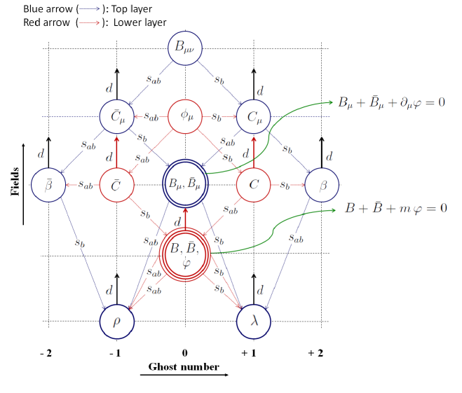
Figure 1: Emergence of CF-type conditions.

In the above paragraph, we have discussed the possible existence of CF-type restrictions in the case of (anti-)BRST symmetry transformations through the diagram (cf. Fig. 1) and demonstrated that the clustering of fields at a point (with the same ghost number) ensures the emergence of CF-type restrictions/conditions (which are the decisive features of a quantum gauge theory within the framework of BRST formalism). In our present theory, there are nilpotent and absolutely anticommuting (anti-)co-BRST symmetry transformations, too. These latter symmetries are absolutely anticommuting only on a hypersurface in the 4D Minkowaskian spacetime manifold where the CF-type restrictions (i.e. ${\cal B}_{\mu}+\bar{\cal B}_{\mu}+\partial_{\mu}\tilde{\varphi}=0$, ${\cal B}+\bar{\cal B}+m\tilde{\varphi}=0$) are satisfied. Diagrammatically (cf. Fig. 2), the emergence of such kind of restrictions can be also discussed along exactly similar lines of arguments as we have demonstrated, the emergence of the CF-type restrictions, in the context of (anti-)BRST symmetry transformations (Fig. 1). There is a decisive and distinct difference, however. We note that, in the case of (anti-)co-BRST symmetry transformations (i.e. $s_{(a)d}B_{\mu\nu}$) for the Abelian 2-form field, we have the relationships: $s_{d}B^{(2)}=*d\bar{C}^{(1)}$ and $s_{ad}B^{(2)}=*dC^{(1)}$ (where $B^{(2)}=\frac{1}{2!}(dx^{\mu}\wedge dx^{\nu})B_{\mu\nu}$, $C^{(1)}=dx^{\mu}C_{\mu}$ and $\bar{C}^{(1)}=dx^{\mu}\bar{C}_{\mu}$) which are different from the (anti-)BRST symmetry transformations where we have: $s_{b}B_{\mu\nu}=dC^{(1)}$ and $s_{ab}B_{\mu\nu}=d\bar{C}^{(1)}$.

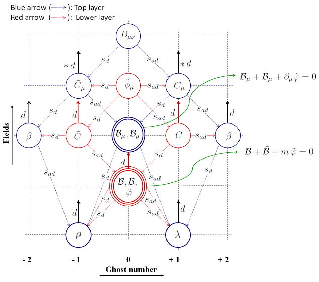
Figure 2: Emergence of CF-type conditions.

In Our earlier works [47, 48], we have established the connection between the CF-type restrictions and the geometrical objects called gerbes. This deep connections physically imply the linear independence of the BRST and anti-BRST symmetry transformations and their corresponding BRST and anti-BRST charges. A similar kind of mathematical connection can be established for the CF-type restrictions, existing in the case of (anti-)co-BRST symmetry transformations (and their corresponding charges) and the ideas of gerbes. We are working in this direction and our results would be reported elsewhere [64].

References

• [1] C. Becchi, A. Rouet, R. Stora, Phys. Lett. B 52 (1974) 344.
• [2] C. Becchi, A. Rouet, R. Stora, Comm. Math. Phys. 42 (1975) 127.
• [3] C. Becchi, A. Rouet, R. Stora, Ann. Phys. (N. Y.) 98 (1976) 287.
• [4] I.V. Tyutin, Lebedev Institute Preprint, Report No.: FIAN-39, (1975),
arXiv:0812.0580[hep-th].
• [5] R.P. Malik, Int. J. Mod. Phys. A 22 (2007) 3521.
• [6] R. Kumar, S. Krishna, A. Shukla, R.P. Malik, Int. J. Mod. Phys. A 29 (2014) 1450135.
• [7] T. Eguchi, P.B. Gilkey, A. Hanson, Phys. Rep. 66 (1980) 213.
• [8] S. Mukhi, N. Mukanda, Introduction to Topology, Differential Geometry and Group Theory for Physicists Wiley Eastern Private Limited, New Delhi, 1990.
• [9] J.W. van Holten, Phys. Rev. Lett. 64 (1990) 2863.
• [10] S. Deser, A. Gomberoff, M. Henneaux, C. Teitelboim,
Phys. Lett. B 400 (1997) 80.
• [11] R.P. Malik, Mod. Phys. Lett. A 14 (1999) 1937.
• [12] R.P. Malik, J. Phys. A: Math. Gen. 33 (2000) 2437.
• [13] R.P. Malik, Mod. Phys. Lett. A 15 (2000) 2079.
• [14] S. Gupta, R. Kumar, R.P. Malik, Eur. Phys. J. C 65 (2010) 311.
• [15] S. Gupta, R.P. Malik, Eur. Phys. J. C 58 (2008) 517.
• [16] R. Kumar, S. Krishna, A. Shukla, R.P. Malik,
Eur. Phys. J. C 72 (2012) 1980.
• [17] R.P. Malik, J. Phys. A: Math. Gen. 34 (2001) 4167.
• [18] E. Witten, Nucl. Phys. B 202 (1982) 253.
• [19] A.S. Schwarz, Lett. Math. Phys. 2 (1978) 247.
• [20] R.P. Malik, J. Phys. A: Math. Gen. 36 (2003) 5095.
• [21] R.P. Malik, Mod. Phys. Lett. A 16 (2001) 477.
• [22] T. Bhanja, D. Shukla, R.P. Malik, Eur. Phys. J. C 73 (2013) 2535.
• [23] S.M. Carroll, Living Rev. Rel. 4 (2001) 1.
• [24] V. Sahani, Lect. Notes Phys. 653 (2004) 141.
• [25] G. Bertone, D. Hooper, J. Silk, Phys. Rep. 405 (2005) 279.
• [26] R. Caldwell, E.V. Linder, Phys. Rev. Lett. 95 (2005) 141301.
• [27] D.N. Spergel et al., Astrophys. J. Suppl. 148 (2003) 175.
• [28] A. G. Riess et al., Astron. J. 116 (1998) 1009.
• [29] S. Perlmutter et al., Astrophys. J. 517 (1999) 565.
• [30] M. Tegmark et al., Phys. Rev. D 69 (2004) 103501.
• [31] K. Abazajian, et al., Astron. J. 126 (2003) 2081.
• [32] K. Abazajian, et al., Astron. J. 128 (2004) 502.
• [33] R.R Caldwell, Phys. Lett. B 545 (2002) 23.
• [34] W.G. Gibbons, Report No.: DAMTP-2003-19, arXiv: hep-th/0302199.
• [35] S.M. Carroll, M. Hoffman, M. Trodden, Phys. Rev. D 68 (2003) 023509.
• [36] V.M. Zhuravlev, D. A. Kornilov, E. P. Savelova,
Gen. Rel. Grav. 36 (2004) 1719.
• [37] M. Li, B. Feng, X. Zhang, JCAP 0512 (2005) 002.
• [38] S. Gupta, R.P. Malik, Eur. Phys. J. C 68 (2010) 325.
• [39] R. Kumar, A. Shukla, Euro. Phys. Lett. 115 (2016) 21003.
• [40] V.I. Ogievetsky, I.V. Polubarinov, Yad. Fiz. 4 (1968) 210.
• [41] M. Kalb, P. Ramond, Phys. Rev. D 9 (1974) 2273.
• [42] R.K. Kaul, Phys. Rev. D 18 (1978) 1127.
• [43] R. Kumar, S. Krishna, Eur. Phys. J. C 77 (2017) 387.
• [44] P.A.M. Dirac, Lectures on Quantum Mechanics, Belfer Graduate School of Science, Yeshiva University Press, New York, 1964.
• [45] K. Sundermeyer, Constrained Dynamics: Lecture Notes in Physics,
Vol. 169, Springer, Berlin, 1982.
• [46] R.P. Malik, T. Pradhan, Z. Phys. C 28 (1985) 525.
• [47] L. Bonora, R.P. Malik, Phys. Lett. B 655 (2007) 75.
• [48] L. Bonora, R.P. Malik, J. Phys. A: Math. Theor. 43 (2010) 375403.
• [49] V.F. Mukhanov, H.A. Feldman, R.H. Brandenberger,
Phys. Rep. 215 (1992) 203.
• [50] S. Mukohyama, Phys. Rev. D 71 (2005) 104019.
• [51] N. Arkani-Hamed, H.C. Cheng, M. A. Luty, S. Mukohyama,
JHEP 0405 (2004) 074.
• [52] A. Adams, N. Arkani-Hamed, S. Dubovsky, A. Nicolis, R. Rattazzi,
JHEP 0610 (2006) 014.
• [53] D. Krotov, C. Rebbi, V.A. Rubakov, V. Zakharov,
Phys. Rev. D 71 (2005) 045014.
• [54] K. Koyama, Class. Quant. Grav. 24 (2007) R231.
• [55] J.D. Barrow, C.G. Tsagas, Class. Quant. Grav. 26 (2009) 195003.
• [56] G. Dvali, A. Franca, C. Gomez, arXiv:1204.6388[hep-th].
• [57] P.J. Steinhardt, N. Turok, Phys. Rev. D 65 (2002) 126003.
• [58] P.J. Steinhardt, N. Turok, Science 296 (2002) 1436.
• [59] M. Novello, S.E.P. Bergliaffa, Phys. Rep. 463 (2008) 127.
• [60] J.L. Lehners, Phys. Rept. 465 (2008) 223.
• [61] Y.F. Cai, D.A. Easson, R. Brandenberger, JCAP 1208 (2012) 020.
• [62] Y.F. Cai, A. Marcianò, D.G. Wang, E.W. Ewing, Universe 3 (2017) 1.
• [63] S. Alexander, S. Cormack, M. Gleiser, Phys. Lett. B 757 (2016) 247.
• [64] S. Krishna, R. Kumar, R.P. Malik (in preparation).