Residual stresses in metal deposition modeling:
discretizations of higher order

Abstract

This article addresses the research question if and how the finite cell method, an embedded domain finite element method of high order, may be used in the simulation of metal deposition to harvest its computational efficiency. This application demands for the solution of a coupled thermo-elasto-plastic problem on transient meshes within which history variables need to be managed dynamically on non-boundary conforming discretizations. To this end, we propose to combine the multi-level $hp$-method and the finite cell method. The former was specifically designed to treat high-order finite element discretizations on transient meshes, while the latter offers a remedy to retain high-order convergence rates also in cases where the physical boundary does not coincide with the boundary of the discretization. We investigate the performance of the method at two analytical and one experimental benchmark.

1 Introduction

The process of metal additive manufacturing involves a highly localized heat source which moves over a substrate. Its purpose is to change the state of the deposited metal either from powder to liquid or from solid to liquid such that the added material bonds with the substrate. The subsequent, rapid cooling of the heat affected zone induces undesired residual stresses, a process well understood in welding, see for example [1, 2]. The numerous physical phenomena involved in this process range from the simplified view stated above to models including detailed weld pool dynamics [3], to models resolving the micro-structure evolution in the cooling phase (see e.g.  [4, 5, 6]). The necessary compromise between the complexity of the physical model and the ever increasing yet limited resources for its numerical resolution is mainly driven by the concrete question which needs to be answered by the simulation, (see e.g. [7] for a guideline in welding).

In this context, efficient numerical discretizations are desirable of which the finite element method is the most prominent choice. A simple measure of its complexity is the number of degrees of freedom involved in the computation. These represent the unknown coefficients of piecewise polynomials spanned on a mesh of finite elements which resolve the highly localized gradients. Three basic strategies are available to control the number of degrees of freedom: a) $h$-refinement, i.e. an increase of the number of finite elements in the mesh, b) $p$-refinement, i.e. an increase of the polynomial degree of each finite element or c) the combination of both: $hp$-refinement. The achievable rate of convergence increases from a) to c) for problems with locally high gradients. Unfortunately, so does the complexity of the implementation of the respective method. This is especially the case in transient problems where the necessary adaptions need to be kept local to the (traveling) heat affected zone.

Numerous approaches are reported in literature for locally $h$-refined discretizations, see e.g. [8] as a representative of an early work on the subject in the context of welding and [9] for a recent review of the available variants applied to metal additive manufacturing including a review of commercial packages for this purpose. Refinements in $p$ beyond quadratic shape functions are scarce, but e.g. [10] demonstrates that it is possible to construct efficient discretizations for elasto-plastic problems by using high order discretizations whose boundary follows the plastic front. The application of $hp$-adaptive methods in this context is e.g. discussed in [11] where exponential convergence rates were achieved for boundary-conforming discretization. Recently, high-order $h$ refinements have also become of interest in the context of Isogeometric Analysis, see e.g. [12]. All these publications treat boundary conforming discretizations. Extensions to non-boundary conforming finite element discretizations are presented in [13, 14] in the context of the finite cell method. Therein, it is demonstrated that high-order convergence rates may also be achieved even if the physical boundaries of the domain do not coincide with the discretization of the mesh. This is a desirable feature in the application at hand where the physical domain grows with time. Additionally, highly localized gradients need to be followed dynamically though the course of the simulation.

As a remedy for an accurate resolution of transient gradients on non-boundary conforming domains we advocate a combination of both, the multi-level $hp$-method and the finite cell method. To this end, we first introduce these numerical methods in section 2 where we begin by recalling the multi-level $hp$-method. It offers a relatively simple management of the degrees of freedom for transient discretizations of $hp$-type. Additionally, we present some novel but straight-forward extensions necessary for elasto-plastic computations on transient discretizations of $hp$-type. We then present the computation of elasto-plasticity in the framework of the finite cell method [15] and proceed to a short description of the thermo-elasto-plastic problem in section 2.3 .

After the basics of the numerical methods are presented, we evaluate their performance against three benchmark examples. In section 3.1 a sphere under internal pressure in which a plastic front evolves is investigated. While the exact location of the plastic front is known in this specific case, in a more general setting it would not be unknown. We, thus, chose a grid-like discretization whose boundaries neither coincide with the evolving plastic front nor with the physical boundaries of the problem setup itself. We demonstrate that it is possible to capture the plastic front and the stress states on non-boundary conforming domains using higher order $h-$ refinements and obtain higher order convergence rates. We then move to the thermo-elasto-plastic setting in section 3.2 to make the point that it is also possible to capture the plastic stress states in a coupled setting accurately. The final numerical example presented in section 3.3 is chosen to demonstrate that the presented methodology is also capable of reproducing stress states of real experiments. We conclude the article by pointing out the potential and limits of the presented approach in section 4 .

2 Numerical Methods

This section serves to introduce and further develop the numerical techniques which are used and evaluated in section 3 . To this end, the multi-level $hp$-method is first presented in section 2.1 followed by a description on the finite cell method section 2.2 . They are then combined to solve problems in elasto-plasticity as introduced in section 2.3 . All these sections form the background for solving thermo-elasto-plastic problems as introduced in section 2.4 .

2.1 The multi-level hp-method

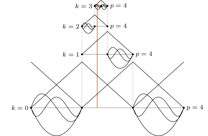
(a) One-dimensional case

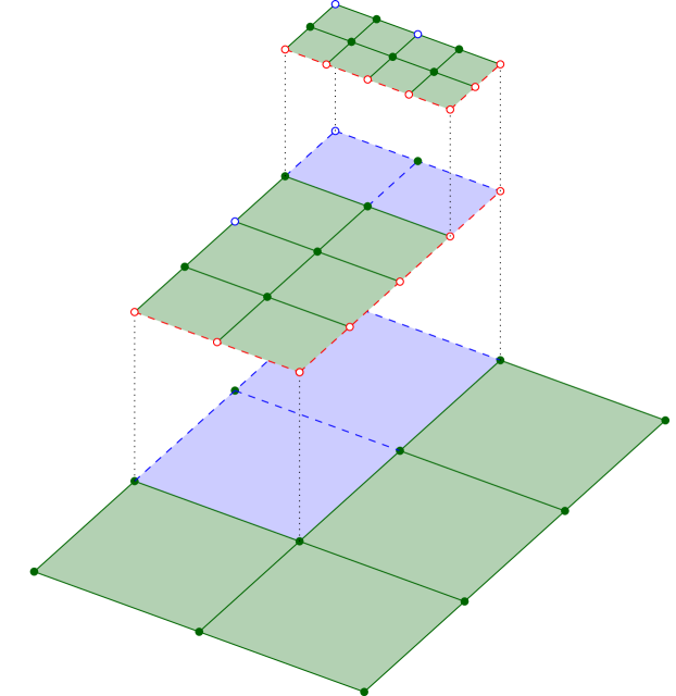
(b) Two-dimensional case

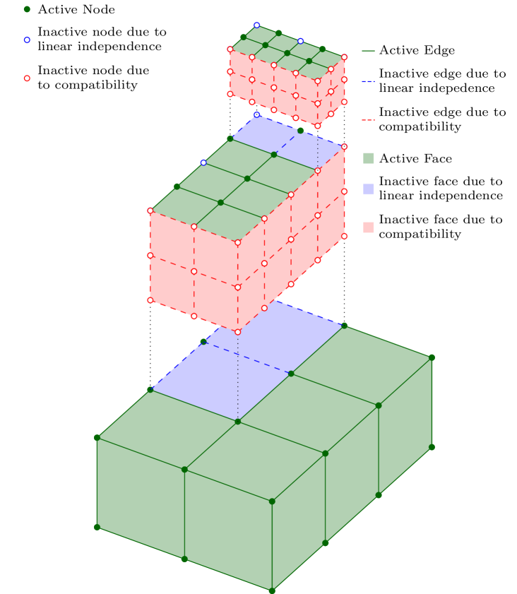
(c) Three-dimensional case

Figure 1: Main idea of the multi-level hp-method in different spatial dimensions [16].

The aforementioned multi-level hp-method is a powerful scheme for performing local mesh adaptation in an efficient manner. It was first introduced in [17] and aims at a simple degree of freedom management for dynamic discretizations of high order by performing local refinements based on superposition. For this purpose, an initial discretization of coarse base elements is overlayed locally with multiple layers of finer overlay elements so as to better capture the solution behavior such as locally high gradients, see fig. 1 . This is in contrast to standard $hp$-methods which perform refinement by replacement where coarse elements are replaced by a set of smaller elements.

The methodology to overlay finite elements as in the multi-level $hp$-method requires the enforcement of linear independence of the basis functions and compatibility of the ansatz space at the boundary of the refinement zone. This is achieved in a straightforward manner by leveraging the direct association of topological components (nodes, edges, faces, volumes) with the degrees of freedom. Compatibility and linear independence are ensured through the deactivation of specific topological components. This deactivation is governed by simple rule-sets, which work for different spatial dimensions [17, 16] alike. This forms a key strength of the method as compared to classic $hp$-methods as the simplicity of the rule-sets allow for an easy treatment of dynamic meshes with arbitrary levels of hanging nodes. The multi-level $hp$-method results in $C^{0}$-continuity over the complete refinement hierarchy in base elements while $C^{\infty}$-continuity is obtained in the leaf elements — elements on the highest refinement level with no children.

2.2 The finite cell method

The ultimate in the scope of this article is to provide a framework which leaves as much geometric and topological freedom for the emerging additively manufactured artifact as possible. At the same time, the effort for mesh generation should be kept as low as possible. These are two main features of immersed methods, a class of advanced discretization techniques that significantly reduce the effort of mesh generation by utilizing a non-boundary conforming domain discretization. They have, therefore, emerged as the method of choice to perform numerical simulations on bodies with a complex shape, topology or a combination of both. The finite cell method (FCM) introduced in [18, 19], is a prominent representative of immersed methods whose core idea is to combine the advantages of the fictitious domain approach with the computational efficiency of discretizations of high order. Its basic idea is depicted in fig. 2 . A body of complex shape and topology defined on a physical domain $\Omega_{\text{phys}}$ is extended by a fictitious domain $\Omega_{\text{fict}}$. Their union yields a computational domain $\Omega=\Omega_{\text{phys}}\cup\,\Omega_{\text{fict}}$ with a simple boundary which can be discretized using well shaped finite elements. These form the support of the ansatz functions and are termed finite cells as their boundary is not conforming to the boundary of the original, physical boundary $\partial\Omega_{\text{phys}}$. The physical domain must then be recovered at the level of the numerical integration of the associated bi-linear and linear forms. An indicator function $\alpha$ is introduced to classify points belonging to the physical or fictitious domain. Points within the physical domain are assigned a value $\alpha=1$, whereas points in the fictitious domain have a value $\alpha\ll 1$.

Figure 2: Core idea of the finite cell method.

While a detailed description of the FCM can be found in [18, 15, 19], the short and concise rehearsal of its basic ideas above suffices to set the stage for its extension to elasto-plastic problems as laid out in the next section.

2.3 Elasto-plasticity with the multi-level hp method

The stage is now set to develop an efficient elasto-plastic formulation which combines the multi-level $hp$-method with the finite cell method as presented in sections 2.1 and 2.2 .

The finite cell method has already been successfully used in the field of plasticity. The work most relevant to the paper at hand is published in [20] in which the FCM was implemented for the $J_{2}$ flow theory with nonlinear, isotropic hardening for small displacements and small strains. Further, in [13] it is demonstrated that the FCM leads to more efficient discretizations than the standard, boundary conforming $h$-version of the finite element method delivers. The FCM has recently also been extended to nearly incompressible finite strain plasticity with complex geometries, see [14]. All these investigations were carried out on static discretizations in the sense that no dynamic refinement was applied locally to capture transient plastic fronts. However, in layered deposition modeling the size of the traveling heat source is comparatively small w.r.t. the rest of the computational domain. In these applications, a dynamic refinement and coarsening offers a discretizational advantage because the computational effort can thereby be balanced with the accuracy needed locally. However, this requires a dynamic management of primal and internal variables.

To facilitate a comprehensive but concise presentation of this subject, the next sections start with the classic formulation of $J_{2}$ plasticity in 2.3.1 . The standard setting is then cast into the FCM formalism in section 2.3.2 before the integration of the multi-level $hp$-method into the elasto-plastic FCM framework is treated in section 2.3.3 along with the associated management of primal and internal variables.

2.3.1 Classic $J_{2}$ plasticity

The classic weak form of equilibrium in a solid body is given by

$$G(\textbf{{u}},\bm{{\eta}})=\int\limits_{\Omega}\bm{{\varepsilon}}(\bm{{\eta}}):\bm{{\sigma}}\,\mathrm{d}\Omega-\int\limits_{\Omega}\bm{{\eta}}\cdot\textbf{{b}}\,\mathrm{d}\Omega-\int\limits_{\Gamma_{N}}\bm{{\eta}}\cdot\textbf{{t}}\,\mathrm{d}\Gamma=0,$$ (1)

where u is the displacement field, $\bm{{\eta}}$ is the test function, $\bm{{\sigma}}$ the Cauchy stress tensor, $\bm{{\varepsilon}}$ the strain tensor, b are the body forces acting on the domain, $\Omega$, and t is the prescribed traction on the Neumann boundary, $\Gamma_{N}$. When a nonlinear material is utilized, the stress state is not only a function of the instantaneous strain. Instead, the stress state also depends on the history of the loads the body was subjected to. Consequently, the weak form (1) becomes nonlinear and is solved incrementally for each time step $[t_{n},t_{n+1}]$. Within each time step the internal variables, $\bm{{\lambda}}$, which contain the history of the material, are assumed constant. Linearization of the weak form with respect to the unknown u around $\textbf{{u}}_{n+1}^{(i)}$ , which is the solution at iteration i, is given e.g. in [21] and reads

$$\int\limits_{\Omega}\bm{{\varepsilon}}(\bm{{\eta}}):\bm{{D}}:\bm{{\varepsilon}}(\delta\textbf{{u}})\,\mathrm{d}\Omega=-\int\limits_{\Omega}\bm{{\varepsilon}}(\bm{{\eta}}):\bm{{\sigma}}_{n+1}(\bm{{\lambda}}_{n},\bm{{\varepsilon}}(\textbf{{u}}_{n+1}^{(i)}))\,\mathrm{d}\Omega$$ (2)

$$+\int\limits_{\Omega}\bm{{\eta}}\cdot\textbf{{b}}_{n+1}\,\mathrm{d}\Omega+\int\limits_{\Gamma_{N}}\bm{{\eta}}\cdot\textbf{{t}}_{n+1}\,\mathrm{d}\Gamma.$$

where the fourth order tensor $\bm{{D}}$ is the tangent modulus defined as

$$\bm{{D}}=\left.\frac{\partial\bm{{\sigma}}_{n+1}}{\partial\bm{{\varepsilon}}}\right|_{\bm{{\varepsilon}}(\textbf{{u}}_{n+1}^{(i)})}.$$ (3)

2.3.2 The elasto-plastic finite cell method

In order to apply the finite cell method, the domain integrals in eq. 2 are multiplied with the indicator function $\alpha$ such that

$$\int\limits_{\Omega}\alpha\,\bm{{\varepsilon}}(\bm{{\eta}}):\bm{{D}}:\bm{{\varepsilon}}(\delta\textbf{{u}})\,\mathrm{d}\Omega=-\int\limits_{\Omega}\alpha\,\bm{{\varepsilon}}(\bm{{\eta}}):\bm{{\sigma}}_{n+1}(\bm{{\lambda}}_{n},\bm{{\varepsilon}}(\textbf{{u}}_{n+1}^{(i)}))\,\mathrm{d}\Omega$$ (4)

$$+\int\limits_{\Omega}\alpha\,\bm{{\eta}}\cdot\textbf{{b}}_{n+1}\,\mathrm{d}\Omega+\int\limits_{\Gamma_{N}}\bm{{\eta}}\cdot\bar{\textbf{{t}}}_{n+1}\,\mathrm{d}\Gamma.$$

Since the solution in the fictitious domain is unphysical, computing the tangent modulus or stresses in the fictitious domain causes unnecessary computational overhead. Therefore, the deformation in the fictitious domain is neglected and stresses are assumed to be zero ($\bm{{\sigma}}_{fict}=\bm{{0}}$). Moreover, the tangent modulus is taken as the elastic tangent ($\bm{{D}}_{fict}=\bm{{D}}^{e}$). Incorporating these assumptions into eq. 4 provides the following linearized weak form of equilibrium for elasto-plastic problems

$$\int\limits_{\Omega_{\text{phys}}}\bm{{\varepsilon}}(\bm{{\eta}}):\bm{{D}}:\bm{{\varepsilon}}(\delta\textbf{{u}})\,\mathrm{d}\Omega+\int\limits_{\Omega_{\text{fict}}}\alpha\,\bm{{\varepsilon}}(\bm{{\eta}}):\bm{{D}}^{e}:\bm{{\varepsilon}}(\delta\textbf{{u}})\,\mathrm{d}\Omega=$$ (5)

$$-\int\limits_{\Omega_{\text{phys}}}\bm{{\varepsilon}}(\bm{{\eta}}):\bm{{\sigma}}_{n+1}(\bm{{\lambda}}_{n},\bm{{\varepsilon}}(\textbf{{u}}_{n+1}^{(i)}))\,\mathrm{d}\Omega+\int\limits_{\Omega}\alpha\,\bm{{\eta}}\cdot\textbf{{b}}_{n+1}\,\mathrm{d}\Omega+\int\limits_{\Gamma_{N}}\bm{{\eta}}\cdot\bar{\textbf{{t}}}_{n+1}\,\mathrm{d}\Gamma.$$

In this paper, a rate-independent von Mises plasticity model with nonlinear isotropic hardening is considered whereby the displacements and strains are assumed to be small. The classic, additive decomposition of the strain tensor into an elastic and a plastic counterpart is then applied such that

$$\bm{{\varepsilon}}=\bm{{\varepsilon}}^{e}+\bm{{\varepsilon}}^{p}.$$ (6)

Figure 3 summarizes this model, in which the internal variables $\bm{{\lambda}}$ are given by

$$\bm{{\lambda}}=\{\,\bm{{\varepsilon}}^{p},\bar{\varepsilon}^{p}\,\},$$ (7)

where $\bar{\varepsilon}^{p}$ is the equivalent plastic strain.

1. Linear elastic law:

   $$\bm{{\sigma}}=\bm{{D}}^{e}:\bm{{\varepsilon}}^{e}$$

2. Yield function:

   $$\Phi=\Phi(\bm{{\sigma}},\bar{\varepsilon}^{p})=\sqrt{3\,J_{2}(\bm{{s}}(\bm{{\sigma}}))}-\sigma_{y}(\bar{\varepsilon}^{p})$$

3. Plastic flow rule:

   $$\dot{\bm{{\varepsilon}}}^{p}=\dot{\gamma}\sqrt{\frac{3}{2}}\,\frac{\bm{{s}}}{\sqrt{\bm{{s}}:\bm{{s}}}}$$

4. Hardening law:

   $$\dot{\bar{\varepsilon}}^{p}=\dot{\gamma}=\sqrt{\frac{2}{3}\,\dot{\bm{{\varepsilon}}}^{p}:\dot{\bm{{\varepsilon}}}^{p}}.$$

5. Kuhn-Tucker conditions:

   $$\Phi\leq 0,\quad\dot{\gamma}\geq 0,\quad\dot{\gamma}\Phi=0$$

Figure 3: Summary of the rate-independent von Mises associative model with nonlinear isotropic hardening

2.3.3 Multi-level $hp$-adaptivity and the transfer of primary and internal variables

In the case of dynamic multi-level hp-refinements the primary variables given by the displacement field, u, and internal variables given by $\bm{{\lambda}}$, need to be transferred from the old discretization prior to the refinement to the new discretization after the refinement was carried out. Since the displacement field over the domain is discretized by the basis functions, a global $C^{0}$ continuous description is available which is directly transferred to the new discretization by means of a global $L_{2}$-projection. However, in the general elasto-plastic finite element procedure, the evolution of the internal variables is computed at local integration points via the plastic flow rule and the hardening law. As no $C^{0}$ continuous discretization is readily available, the transfer of these variables from the integration points of the old discretization to the integration points of the new one is more involved.

As a remedy, several strategies have been developed in literature. The simplest is the point-wise transfer of the internal variables [22]. Therein, an area is associated to each old integration point within which constant values of the history variables are assumed. This leads to a discontinuous approximation of the history variables within the concerned finite elements. Another strategy is the element-wise transfer [23], where the internal variables are interpolated by local functions. This strategy can result in an approximation with discontinuities over element boundaries. A cure is offered by the large group of strategies involving nodal projections. Therein the internal variables are first transferred from integration points of the old discretization to the nodal degrees of freedom of that old discretization. This is achieved in [22] and [24] by extrapolating the values from integration points to the nodal dofs for each element locally and later averaging these extrapolated values. Another possibility is to use the super convergent patch recovery technique as presented in [25, 26, 27, 28], for the transfer of the values from the integration points of the old mesh to its nodes. In this approach a patch consists of elements that surround a node and the internal variables are fitted to continuous polynomials over each patch by a least squares method and are then interpolated to the nodal points. Independent of how the values are obtained at the nodes of the old discretization, the next step is to interpolate them to the new nodal points in the new mesh. Finally, the values of the internal variables at the new integration points are interpolated from the values of the new nodal points. Since this strategy acts as a smoothing operator, the localized internal variables are smeared out over a larger part of the domain. This can be a drawback in elasto-plastic analysis, because plasticity is a local effect in most cases.

Unfortunately, none of these techniques are suitable for the multi-level hp-adaptivity. This is mainly due to the fact that the high order basis functions are modal functions, which are not associated to specific nodes. For this reason a modified version of the element-wise transfer [23] is advocated in the paper at hand in which each component of the internal variables, $\lambda_{i}$, is approximated such that

$$\lambda_{i}\approx\lambda^{h}_{i}=\mathbf{P}(r,s,t)\,\mathbf{c}$$ (8)

where $\mathbf{P}$ is a vector of integrated Legendre polynomials as used in p-version of FEM [29] and $\mathbf{c}$ is the corresponding coefficient vector. It is explicitly pointed out that these polynomials only span the leaf element, where $(r,s,t)$ denotes the local coordinates of this element. The coefficient vector, $\mathbf{c}$ is determined by applying a least square fit to the discrete integration point values, $\lambda^{d}_{i}(r_{j},s_{j},t_{j})$, inside the leaf element. This is done by minimizing the function, $F(\mathbf{c})$,

$$F(\mathbf{c})=\sum_{j=1}^{n_{gp}}\big{(}\lambda^{d}_{i}(r_{j},s_{j},t_{j})-\mathbf{P}(r_{j},s_{j},t_{j})\,\mathbf{c}\big{)}^{2},$$ (9)

which is carried out by differentiating $F$ with respect to $\mathbf{c}$ as

$$\frac{\partial F}{\partial\mathbf{c}}=\mathbf{b}-\mathbf{A}\,\mathbf{c}=0,$$ (10)

with

$$\mathbf{A}=\sum_{j=1}^{n_{gp}}\mathbf{P}^{T}(r_{j},s_{j},t_{j})\,\mathbf{P}(r_{j},s_{j},t_{j}),\quad\mathbf{b}=\sum_{j=1}^{n_{gp}}\mathbf{P}^{T}(r_{j},s_{j},t_{j})\,\lambda^{d}_{i}(r_{j},s_{j},t_{j}).$$ (11)

Equation (10) leads to the following linear system of equations

$$\mathbf{A}\,\mathbf{c}=\mathbf{b},$$ (12)

which needs to be solved for each component of the internal variables.

If this projection strategy is applied to the elements that contain the plastic front, i.e. in which only a group of integration points in the element accumulated plastic strains, then the proposed least squares approximation may lead to oscillations and spurious values. In some cases it is even possible to obtain invalid negative values for the equivalent plastic strain. Figure 4 illustrates this for the polynomial order $p=4$ for a simple one dimensional example in which the equivalent plastic strain should be nonzero for the two plastified integration points and zero for the three elastic integration points. This function cannot be represented by polynomials and the well known Gibbs phenomenon occurs.

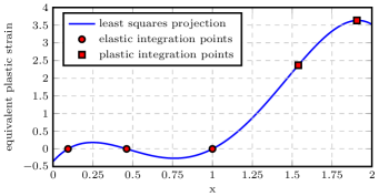
Figure 4: Convergence

In order to circumvent this problem, the values in those elements containing a elastic-plastic interface are not projected with the least squares method. Instead, for these elements we advocate the following approach depicted in Figure 5a . Four cases are distinguished and characterized by the location of the integration points w.r.t. the concerned interpolation point. The first case is given in Figure 5b where the interpolation point $p_{1}$ is located inside the gray bounding box defined by all integration points. In this case the internal variables, $\lambda_{i}$ at $p_{1}$ are approximated by a trilinear interpolation from the values of the eight integration points closely surrounding it. In all the other cases the interpolation point $p$ is located outside the gray bounding box. Therefore, its projection onto the corresponding surface, edge or corner of the bounding box, $p^{*}$, is used for interpolation. Figure 5c depicts the second case in which the projection of $p_{2}$ is surrounded by only four points. These are then used for bilinear interpolation. The third case occurs when the projected point is surrounded by only two points as demonstrated in Figure 5d . In this case linear interpolation is applied. The last case occurs when the original interpolation point lies in the corner quadrants of the finite cell. In this case values at the closest integration point are used. We will demonstrate in section 3 that this approach is feasible for dynamic multi-level $hp$-discretizations in an elasto-plastic setting.

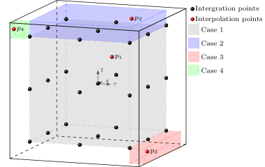
(a) Interpolation cases

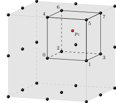
(b) Case 1: Trilinear interpolation

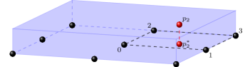
(c) Case 2: Bilinear interpolation

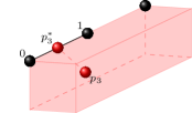
(d) Case 3: Linear interpolation

Figure 5: Interpolation in interface element

2.4 Coupling to thermal problems

Metal deposition is a multi-physics problem, where the highest temperature gradients as well as the phase changes occur in close vicinity of the moving laser beam. The phase changes between liquid and solid states are simulated by the model introduced by Celentano et. al. [30] which uses the discretized weak form of equation (14). Further details regarding this method and its application to thermal analysis of the selective laser melting process in the framework of multi-level hp-adaptivity can be found in  [31].

$$\rho c\frac{\partial T}{\partial t}+\rho L\frac{\partial f_{pc}}{\partial t}-\nabla\cdot(k\nabla T)=Q$$ (13)

A dynamically adaptable data container (multi-level grid) is used to keep track of the physical domain $\Omega_{phys}$ during the deposition process. The container represents a dynamic octree. It stores the current material state of a voxel at all points in time. Material states are stored in this container and not associated to finite elements. This decoupling of material and discretization facilitates the use of the finite cell method.

Due to the changes in the temperature during the process, some regions in the domain expand, while others contract. This generates residual stresses in the part when the thermal load is removed and the material allowed to cool down to its initial temperature. These stresses are computed by the quasi-static mechanical model, given in Section 2.3 with the addition of the thermal strain defined as

$$\bm{{\varepsilon}}^{th}=\gamma\,\Delta T\,\bm{{I}},$$ (14)

where $\gamma$ is the thermal expansion coefficient and $\bm{{I}}$ is the second order identity tensor. Adding the thermal strain component extends the additive decomposition of strains given in equation (6) to

$$\bm{{\varepsilon}}=\bm{{\varepsilon}}^{e}+\bm{{\varepsilon}}^{p}+\bm{{\varepsilon}}^{th}.$$ (15)

It should be noted that, the von Mises plasticity depends solely on the deviatoric part of the strain tensor and the thermal strain is purely hydrostatic. Therefore, the basic structure of the elasto-plastic model introduced in Section 2.3 remains as is. Only the additive decomposition of the strains changes along with the fact that the yield stress and the thermal expansion coefficient are now temperature dependent functions.

Figure 6: Thermomechanical coupling

It is assumed that displacements are small and do not produce heat, so that only a one-directional coupling has to be taken into account, i.e. only the displacement field is affected by the changes in the temperature field. As shown in Figure 6 , a staggered approach is taken for the solution of the thermomechanically coupled problem. For each time step, the multi-level grid is first updated according to the metal deposition such that the physical domain, $\Omega_{phys}$, is defined for both the thermal and the mechanical problems. Then, the thermal problem is solved to obtain the temperature distribution. Finally, the resulting temperature field is used to compute the thermal strains and temperature-dependent material properties used to solve the mechanical problem before the next time step is computed.

3 Numerical Examples

All presented examples have benchmark character and are chosen thoroughly to test the main aspects of the proposed methodology. The first example discussed in section 3.1 is chosen to test if higher order convergence rates are possible in elasto-plastic computations and under what circumstances they decay. To this end, a dynamic multi-level $hp$-refinement as presented in section 2.1 is carried out towards the plastic front in several load steps whereby the plastic front itself is not resolved in a boundary conforming manner but travels through finite cells. This situation is expected for engineering applications. The example also tests the finite cell formulation presented in section 2.2 in the elasto-plastic embedded domain setting as described in section 2.3 by resolving the boundary of the physical domain only on integration level. It also serves as a test for the transfer of history variables as detailed in section 2.3.3 .

The second example given in section 3.2 is chosen to verify the thermo-elasto-plastic coupling procedure laid out in section 2.4 . Both fields are discretized on separate computational grids which are refined and de-refined individually according to the requirements of the corresponding field variable.

The final example presented in section 3.3 tests the combination of the methodology on a experimental benchmark used in welding. As such, it constitutes a first step towards a verification of the proposed methodology for layer deposition modeling.

3.1 Internally pressurized spherical shell

In this example internal pressure, $P$, is applied in increments to a spherical shell, which is composed of an elastic perfectly plastic material with a von Mises yield criterion. Figure 7a illustrates the problem setup, where $r_{i}$, $r_{o}$ and $r_{p}$ are inner radius, outer radius and the radius of the plastic front, respectively.

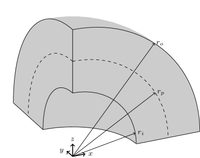
(a) An octant of the spherical shell

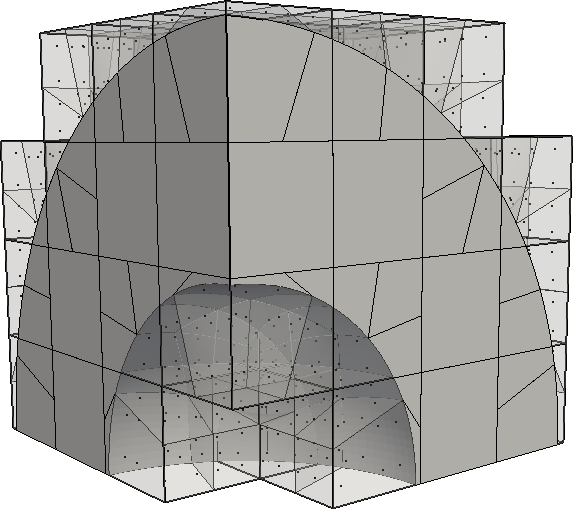
(b) Smart octree integration on $4\times 4\times 4$ base mesh

Figure 7: Set up of internally pressurized sphere

Hill [32] provides an analytical solution to this problem. Equation (16) gives the relation between the location of the plastic front, $r_{p}$, and the applied internal pressure, $P$, wherein $\sigma_{y}$ is the yield stress.

$$P=2\,\sigma_{y}\ln\bigg{(}\dfrac{r_{p}}{r_{i}}\bigg{)}+\dfrac{2\,\sigma_{y}}{3}\bigg{(}1-\dfrac{r_{p}^{3}}{r_{o}^{3}}\bigg{)}$$ (16)

The analytical solutions of the normal stresses in spherical coordinates are provided in equations (17) and (18). The shear components in spherical coordinates are zero.

$$\sigma_{rr}=\begin{cases}-2\,\sigma_{y}\bigg{[}\ln\bigg{(}\dfrac{r_{p}}{r}\bigg{)}+\dfrac{1}{3}\bigg{(}1-\dfrac{r_{p}^{3}}{r_{o}^{3}}\bigg{)}\bigg{]}&\text{if }\,\,r\leq r_{p}\\ \\ -\dfrac{2\,\sigma_{y}\,r_{p}^{3}}{3\,r_{o}^{3}}\bigg{(}\dfrac{r_{o}^{3}}{r^{3}}-1\bigg{)}&\text{if }\,\,r>r_{p}\end{cases}$$ (17)

$$\sigma_{\theta\theta}=\sigma_{\phi\phi}=\begin{cases}2\,\sigma_{y}\bigg{[}\dfrac{1}{2}-\ln\bigg{(}\dfrac{r_{p}}{r}\bigg{)}-\dfrac{1}{3}\bigg{(}1-\dfrac{r_{p}^{3}}{r_{o}^{3}}\bigg{)}\bigg{]}&\text{if }\,\,r\leq r_{p}\\ \\ \dfrac{2\,\sigma_{y}\,r_{p}^{3}}{3\,r_{o}^{3}}\bigg{(}\dfrac{r_{o}^{3}}{2\,r^{3}}+1\bigg{)}&\text{if }\,\,r>r_{p}\end{cases}$$ (18)

Due to symmetry, only an octant of the whole spherical shell is considered in the numerical model with the appropriate symmetry boundary conditions. The shell is embedded in a Cartesian grid of size $4\times 4\times 4$ elements, where finite cells located completely outside the spherical shell are removed from the computation. For the numerical simulations the spherical shell is selected to have an inner radius of $50$ mm and outer radius of $100$ mm. The Young’s modulus, $E$, and Poisson’s ratio, $\nu$, are set to $10$ GPa and $0.3$, respectively, and the yield stress, $\sigma_{y}$, is set to $41.79389833783693$ MPa.

The geometry of the spherical shell is captured at the integration level by utilizing the smart octree algorithm as explained in [33]. Figure 7b illustrates the resulting integration points and cells for base elements.

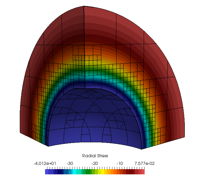
(a) Radial stresses at P = 40 MPa

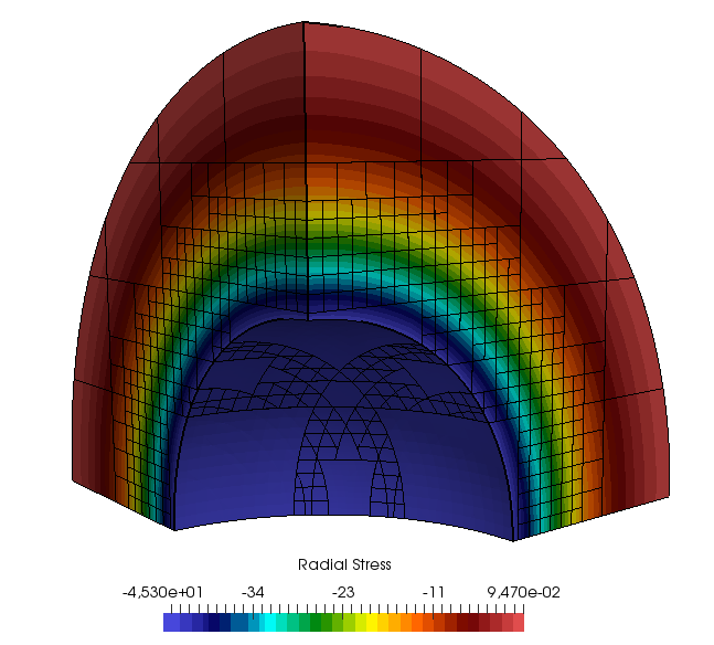
(b) Radial stresses at P = 45 MPa

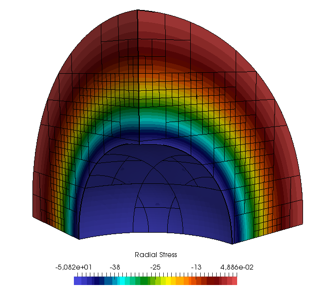
(c) Radial stresses at P = 50 MPa

Figure 8: Radial stresses on a dynamically adaptive multi-level $hp$-discretization with polynomial degree $4$.

Figure 8  shows the distribution of the radial stresses on a dynamically adaptive multi-level $hp$-discretization for three load steps, where the polynomial degree of the basis functions is chosen to be $p=4$ and maximum refinement level is set to $3$. In each step the elements that are close to the plastic front are refined and the elements that are further away from the plastic front are coarsened. Moreover, in each step the primary variables related to degrees of freedom and internal variables at integration points are transferred as explained in Section 2.3.3 .

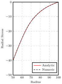
(a) P = 40 MPa

(b) P = 45 MPa

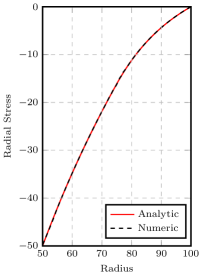
(c) P = 50 MPa

Figure 9: Radial stresses along radius of the spherical shell

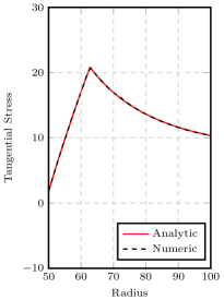
(a) P = 40 MPa

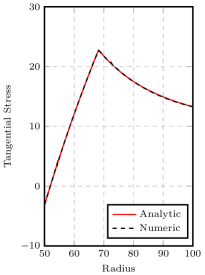
(b) P = 45 MPa

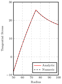
(c) P = 50 MPa

Figure 10: Tangential stresses along the radius of the spherical shell

It can be seen from the equations (17) and (18) that the stresses vary only in $r$-direction and are constant in $\theta$- and $\phi$-directions. Therefore, it is sufficient to compare the computed stresses along the radius of the spherical shell to the analytical stresses as depicted in Figure 9 and Figure 10 . Both radial and tangential stress results obtained from the numerical simulation match their analytical counterparts for each load step. The different material behavior in elastic and plastic regions introduces a kink in the stress field, which is more blatant for the tangential stress. The introduced multi-level $hp$-refinement towards that elastic-plastic interface allows the numerical solution to closely capture this behavior.

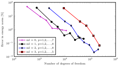
Figure 11: Convergence in energy norm starting from a $4\times 4\times 4$ base mesh with multi-level $hp$ refinement (ml).

In order to investigate the convergence properties of this elasto-plastic problem in the framework of the multi-level $hp$-adaptive finite cell method as described in sections 2.1, 2.2 and 2.3 , p-convergence studies are performed by uniformly elevating the order p of the polynomial shape functions, while keeping the size of the base elements fixed. For these studies a $4\times 4\times 4$ base mesh is used, which is recursively refined towards the elastic-plastic interface. Moreover, an internal pressure $P=50$ MPa is applied in one load step for each computation. To this end, the relative error in energy is monitored, which is defined as

$$e=\sqrt{\dfrac{|U_{ex}-U_{num}|}{U_{ex}}}\times 100,$$ (19)

with the exact internal energy, $U_{ex}$, and the numerical internal energy, $U_{num}$, computed as

$$U=\dfrac{1}{2}\int\limits_{\Omega}\bm{{\varepsilon}}:\bm{{\sigma}}\,\mathrm{d}\Omega.$$ (20)

By using the analytical solutions in equation (20) the exact internal energy for an octant of the spherical shell is obtained as follows

$$U_{ex}=\dfrac{\pi\,P\,\sigma_{y}\,r_{i}^{3}}{4\,E}\bigg{[}(1-\nu)\dfrac{r_{p}^{3}}{r_{i}^{3}}-\dfrac{2}{3}(1-2\,\nu)\bigg{(}1-\dfrac{r_{p}^{3}}{r_{o}^{3}}+3\,\ln\Big{(}\dfrac{r_{p}}{r_{i}}\Big{)}\bigg{)}\bigg{]}.$$ (21)

Figure 11 shows the relative error in energy with respect to the number of degrees of freedom for studies where the maximum refinement level is increased from zero to three. To rule out any domain integration errors, all volumetric integrals were evaluated exactly following [33]. The curve without any multi-level refinement depicts exponential convergence in the pre-asymptotic range until the error is dominated by the kink in the solution field caused by the elastic-plastic interface. This kink is neither resolved by the boundaries of the finite cells nor is the error controlled by a refinement in the vicinity of this irregularity in the solution. Therefore, in the asymptotic range, the error decreases only algebraically when the polynomial degree is further increased. The kink in the solution field is better approximated by the basis functions as the elements are refined towards the elastic-plastic interface with hierarchical multi-level refinement. This can be seen in curves with one and two refinement levels towards the elastic-plastic interface, where the point at which the convergence levels off to its asymptotic value occurs much later. The curve with three refinement levels converges exponentially. Here, the error at the interface does not dominate the overall error.

This demonstrates that the combination of the techniques presented in sections 2.1, 2.2 and 2.3 is able to maintain the expected convergence behavior for higher-order methods even if neither the physical boundaries of an artifact nor an evolving elasto-plastic front are explicitly captured by the boundaries of the discretization.

3.2 Thermo-elasto-plastic bar example

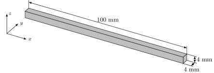
Figure 12: Set up of solidifying bar

In this section, the thermo-mechanical model introduced in Section 2.4 is investigated in the framework of multi-level hp-adaptivity. To this end, an idealized version of the metal casting process is simulated on a semi-infinite bar. Initially, the bar, which is given in Figure 12 , is liquid with a uniform temperature, $T_{i}$. Then, the temperature at the boundary $x=0$ is instantaneously changed to $T_{w}$ and kept constant. $T_{w}$ is lower than the melting temperature, $T_{m}$. Therefore, the bar starts to solidify from this boundary onwards.

The analytical solution to the thermal part of this problem is described in [34] and is known in the literature as Neumanns’s method, see e.g. [35, 36]. The position of the liquid-solid interface is given as

$$X(t)=2\,\lambda\,\sqrt{\alpha\,t},$$ (22)

where $\alpha$ is the diffusivity of the material and $t$ is the time. The constant $\lambda$ is computed by solving the following nonlinear equation

$$\dfrac{e^{-\lambda^{2}}}{\text{erf}(\lambda)}+\dfrac{e^{-\lambda^{2}}\,(T_{m}-T_{i})}{\text{erfc}(\lambda)\,(T_{m}-T_{w})}=\dfrac{\lambda\,L\sqrt{\pi}}{c\,(T_{m}-T_{w})},$$ (23)

where $L$ is the latent heat and $c$ is the heat capacity. The analytical temperature distribution is given in equation (24) for the semi-infinite bar.

$$T(x,t)=\begin{cases}T_{w}+(T_{m}-T_{w})\dfrac{\text{erf}(x/2\sqrt{\alpha t})}{\text{erf}(\lambda)}&\quad\text{if}\quad x\leq X(t)\\ \\ T_{i}+(T_{m}-T_{i})\dfrac{\text{erfc}(x/2\sqrt{\alpha t})}{\text{erfc}(\lambda)}&\quad\text{if}\quad x>X(t)\end{cases}$$ (24)

By using the temperature distribution over the body obtained from the Neumanns’s method, Weiner and Boley [37] developed an analytical solution for the thermal stresses for this problem. They assumed that the body is composed of an elastic perfectly plastic material with a yield stress, $\sigma_{y}$, which linearly decreases as the temperature reaches the melting point, where it becomes zero:

$$\sigma_{y}(T)=\begin{cases}\sigma_{y_{0}}\dfrac{T_{m}-T}{T_{m}-T_{w}}&\quad\text{if}\quad T_{w}\leq T\leq T_{m},\\ \\ 0&\quad\text{if}\quad T>T_{m}.\end{cases}$$ (25)

Moreover, the following dimensionless quantities are introduced,

$$m=\frac{(1-\nu)\,\sigma_{y_{0}}}{\gamma\,E\,(T_{m}-T_{w})},\quad D=\frac{1}{\text{erf}(\lambda)},\quad\hat{x}=\frac{x}{X(t)},\quad\hat{\sigma}=\frac{\sigma\,(1-\nu)}{\gamma\,E\,(T_{m}-T_{w})},$$ (26)

where $E$, $\nu$ and $\gamma$ are Young’s modulus, Poisson’s ratio and thermal expansion coefficient, respectively. The analytical solution of the dimensionless normal stress components in y- and z-directions are then given as

$$\hat{\sigma}_{yy}(\hat{x})=\hat{\sigma}_{zz}(\hat{x})=\begin{cases}m\,[D\,\text{erf}(\lambda\,\hat{x})-1]\hskip 112.00014pt\quad\text{if}\quad 0\leq\hat{x}<\hat{x}_{2}\\ \\ m\,[1-D\,\text{erf}(\lambda\,\hat{x}_{1})]+D\,[\text{erf}(\lambda\,\hat{x}_{1})-\text{erf}(\lambda\,\hat{x})]\\ \quad\quad-\dfrac{2}{\sqrt{\pi}}\,D\,(1-m)\,\lambda\,\hat{x}_{1}\,e^{-\lambda^{2}\hat{x}_{1}^{2}}\,\text{log}(\dfrac{\hat{x}_{1}}{\hat{x}})\hskip 13.00005pt\quad\text{if}\quad\hat{x}_{2}\leq\hat{x}\leq\hat{x}_{1}\\ \\ m\,[1-D\,\text{erf}(\lambda\,\hat{x})]\hskip 111.00023pt\quad\text{if}\quad\hat{x}_{1}<\hat{x}\leq 1\\ \\ 0\hskip 183.0003pt\quad\text{if}\quad\hat{x}>1\end{cases}$$ (27)

where the coordinates $\hat{x}_{1}$ and $\hat{x}_{2}$ denote the elastic-plastic interfaces. According to this solution, the solid material behaves elastic within the range $[\hat{x}_{2},\,\hat{x}_{1}]$ and plastic in ranges $[0,\,\hat{x}_{2}]$ and $[\hat{x}_{1},\,1]$. The positions of these interfaces are obtained by solving the following nonlinear equations

$$2\,(1-m)\,\lambda^{2}\,\hat{x}_{1}\,e^{-\lambda^{2}\hat{x}_{1}^{2}}\,(\hat{x}_{1}-\hat{x}_{2}) =(1+m)\,e^{-\lambda^{2}\hat{x}_{2}^{2}}-(1-m)\,\text{exp}(-\lambda^{2}\,\hat{x}_{1}^{2})-m(e^{-\lambda^{2}}+1),$$ (28)

$$\dfrac{2(1-m)\,\lambda\,\hat{x}_{1}\,e^{-\lambda^{2}\hat{x}_{1}^{2}}}{\sqrt{\pi}}\,\text{log}(\dfrac{\hat{x}_{1}}{\hat{x_{2}}}) =(1-m)\,\text{erf}(\lambda\,\hat{x}_{1})-(1+m)\,\text{erf}(\lambda\,\hat{x}_{2})+2\,m\,\text{erf}(\lambda)$$

The values that are selected for the material properties of this problem are provided in Figure 12 . With these values, the constant $\lambda$ is computed as 0.330825295611989, while the coordinates $\hat{x}_{1}$ and $\hat{x}_{2}$ are found to be 0.45487188 and 0.21570439, respectively.

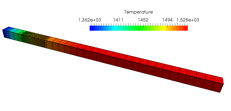
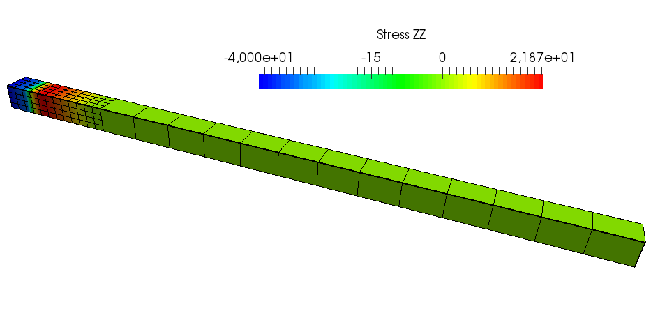
(a) t = 1 second

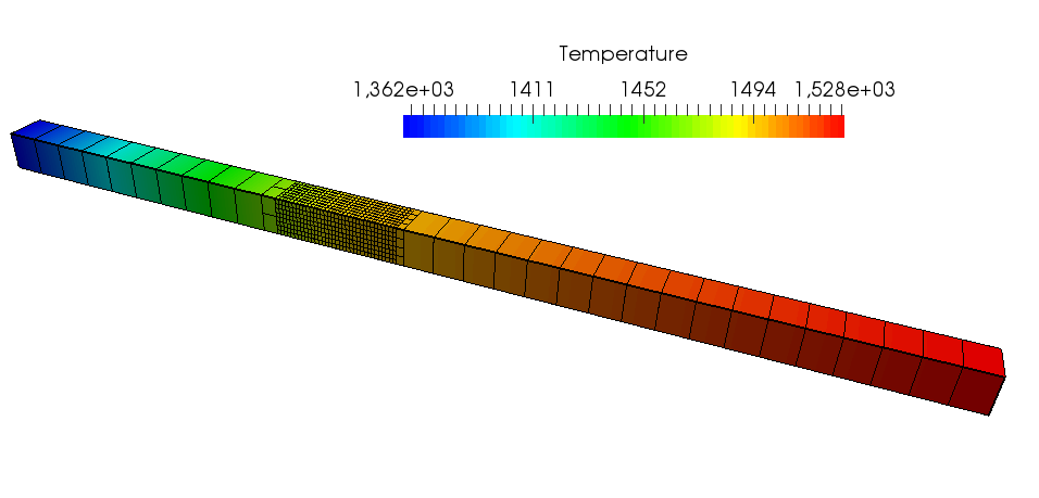
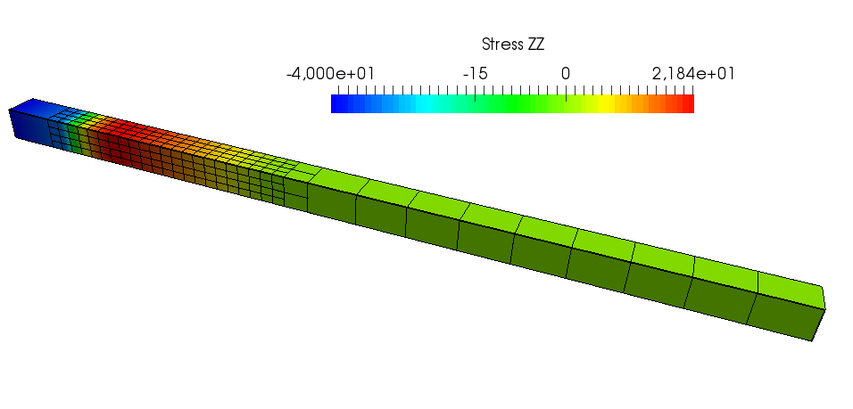
(b) t = 5.1 seconds

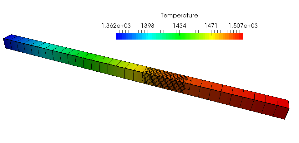
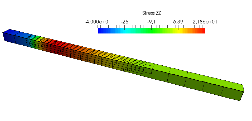
(c) t = 13.2 seconds

Figure 13: Temperature and stress distributions at various time states on dynamically refined thermal and mechanical meshes, respectively

The transient thermal problem is solved on a base mesh with 32 hexahedral elements of order $p=3$ that are distributed in x-direction. Homogeneous Neumann boundary conditions are applied along y- and z-directions and Dirichlet boundary conditions are applied in the yz-plane at $x=0$ and $x=100$. In order to better represent the kink in the temperature field, the elements are dynamically refined three times towards the solid-liquid interface. The time step for the backward Euler scheme is chosen to be $\delta t=0.1$ seconds.

The simulation for the quasi-static mechanical problem is carried out on a base mesh with 16 hexahedral elements of order $p=4$ which are dynamically refined twice towards both the solid-liquid interface and the elastic-plastic interfaces. During the simulation the liquid part of the bar is treated as a fictitious domain as explained in Section 2.2 by multiplying $E$ with $\alpha=10^{-8}$. Extended plane strain conditions are applied along y- and z-directions such that $\varepsilon_{yy}$ and $\varepsilon_{zz}$ are constant. This is achieved by constraining all degree of freedoms corresponding to displacements in y- and z-directions to be equal via Lagrange multipliers. As for the x-direction, the bar is fixed at $x=0$ and left free at $x=100$.

(a) t = 1 second

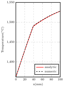
(b) t = 5.1 seconds

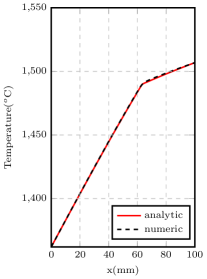
(c) t = 13.2 seconds

Figure 14: Comparison of the numerical and the analytical temperature distribution along x-axis.

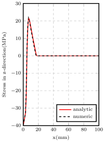
(a) t = 1 second

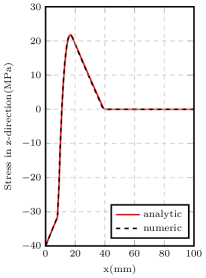
(b) t = 5.1 seconds

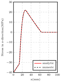
(c) t = 13.2 seconds

Figure 15: Comparison of the numerical and the analytical stress ($\sigma_{zz}$) distribution along x-axis.

Figure 13 presents the results of the thermal and the mechanical problems for the time states $t=\left\{1,5.1,13.2\right\}$ seconds. For the thermal problem the evolution of the temperature field is provided over the dynamically adapted thermal mesh. As for the mechanical problem the stress component in z-direction ($\sigma_{zz}$) is given over the dynamically adapted mechanical mesh. The sequence of figures demonstrates how elements are refined and coarsened during the simulation for thermal and mechanical problems independently.

Figure 14 compares the temperature distribution along the bar to the analytical solution obtained by the Neumanns’s method. The kink in the temperature field at melting temperature, which is caused by the latent heat release during the phase change from liquid to solid, is well captured in all time states as well as the general temperature profile along the bar. The stress component in z-direction ($\sigma_{zz}$) along the bar is depicted in Figure 15 along with the analytical solution provided by Weiner and Boley. The kinks at the elastio-plastic interfaces and the solid-liquid interface are well represented due to refinements. Moreover, it can be seen that the numerical results closely match their analytical counterparts along the bar at all time steps of the computation.

3.3 Applications to metal deposition

In this section the performance of the numerical method introduced in Section 2 in simulating metal deposition processes is investigated against the benchmark problem of a single bead laid down on the top surface of a plate as published in [38]. This benchmark problem is produced by the European Network on Neutron Techniques Standardization for Structural Integrity (NeT), whose mission is to develop experimental and numerical techniques and standards for the reliable characterisation of residual stresses in structural welds. Partners from industry and academia participated in this benchmark by constructing an experiment and measuring the residual stresses on the plate [39, 40, 41, 42, 43] or predicting the residual stresses through numerical methods [44, 39, 45, 46, 40, 47]. Smith et. al. compares the residual stress measurements and predictions of all these groups in [48].

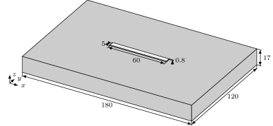
Figure 16: Setup of welding

Figure 16 illustrates the setup of the benchmark problem where the plate has dimensions 180 mm $\times$ 120 mm $\times$ 17 mm in length, width and thickness, respectively. Additionally, the bead that is laid down on the top surface of the plate has a width of 5 mm, thickness of 0.8 mm and a length of 60 mm.

According to the benchmark protocol, the plate and the bead material is AISI Type 316L stainless steel. NeT recommends using slightly different temperature dependent material properties for the parent and weld metal. However, in this work the weld metal is not distinguished from the parent metal. Table 1 provides the temperature dependent specific heat, conductivity, thermal expansion coefficient and Young’s modulus. Over the melting temperature of 1400 °C these values are assumed to be constant. In addition to that the density and Poisson’s ratio are assumed to be constant values of 7966 kg m^-3 and 0.294, respectively and latent heat is taken as 260 kJ/kg. Finally, the monotonic tensile test results, which show the true stress corresponding to the percentage of plastic strain, is given in Table 2 by NeT. The isotropic hardening behaviour of the material is based on this table.

Table 1: Material properties of AISI Type 316L stainless steel [44].

Temperature $[\degree$C]	Specific heat $[$kJ/kg/°C]	Conductivity $[$W/m/°C]	Thermal expansion $[\times 10^{6}$ mm/mm/°C]	Young’s modulus $[$GPa]
20	0.492	14.12	14.56	195.6
100	0.502	15.26	15.39	191.2
200	0.514	16.69	16.21	185.4
300	0.526	18.11	16.86	179.6
400	0.538	19.54	17.37	172.6
500	0.550	20.96	17.78	164.5
600	0.562	22.38	18.12	155.0
700	0.575	23.81	18.43	144.1
800	0.587	25.23	18.72	131.4
900	0.599	26.66	18.99	116.8
1000	0.611	28.08	19.27	100.0
1100	0.623	29.50	19.53	80.0
1200	0.635	30.93	19.79	57.0
1300	0.647	32.35	20.02	30.0
1400	0.659	33.78	20.21	2.0

Table 2: True stress values [MPa] of AISI Type 316L stainless steel at various true plastic strain [40].

Temperature $[\degree$C]	0%	0.2%	1%	2%	5%	10%	20%	30%	40%
23	210	238	292	325	393	494	648	775	880
275	150	173.7	217	249	325	424	544	575
550	112	142.3	178	211	286	380	480	500
750	95	114.7	147	167	195	216	231	236
800	88	112	120	129	150	169	183
900	69	70	71	73	76	81
1100	22.4
1400	2.7

The heat input from the welding torch, which travels with the speed of 2.27 mm$/$s, is defined by NeT as 633 J$/$mm. The moving heat source is based on the Goldak’s [49] ellipsoidal model, which is widely used in welding simulations. In this model the body load is given as

$$q(x,y,z)=\dfrac{6\,\sqrt{3}\,Q}{\pi\,\sqrt{\pi}\,r_{x}\,r_{y}\,r_{z}}\,e^{-3\Big{(}\dfrac{x-x_{c}}{r_{x}}\Big{)}^{2}}\,e^{-3\Big{(}\dfrac{y-y_{c}}{r_{y}}\Big{)}^{2}}\,e^{-3\Big{(}\dfrac{z-z_{c}}{r_{z}}\Big{)}^{2}},$$ (29)

where $x_{c}$, $y_{c}$ and $z_{c}$ define the position of the welding torch and $r_{x}$, $r_{y}$ and $r_{z}$ are the semi-axes of the ellipsoid. Shan et. al.[44] uses the weld bead profile measurements to decide the semi-axes of the ellipsoid, which is followed in this work. According to these measurements $r_{x}$, $r_{y}$ and $r_{z}$ are assumed to be 1.9 mm, 3.2 mm and 2.8 mm, respectively. Moreover, in equation (29) $Q$ is the power of the heat source, which is computed from the heat input and the welding speed as 1437 Watt.

The heat loss from the system is modeled with radiation and convection boundary conditions on the surface of the weld bead and the plate. During the process, the surface is updated as new weld bead is deposited. The convection coefficient and the emissivity are taken as 10 W$/$m²K and 0.75, respectively and they are assumed to be independent of the temperature. Additionally, the ambient temperature is also assumed to be constant at 20 °C.

Figure 17: Setup of welding

Due to symmetry, only half of the plate and the weld bead is considered as shown in Figure 17 for the numerical model with the appropriate symmetry boundary conditions. The plate and the weld bead are embedded in a Cartesian grid of size $30\times 12\times 7$ elements with polynomial order 3 for both the thermal and mechanical problems. The dimensions of the computational domain are 180 mm, 60 mm and 18.6 mm in length, width and thickness, respectively. It should be noted that the thickness of the computational domain is greater than the total thickness of the plate and the weld bead, which is 17.8 mm. The first six rows of elements in thickness are used to discretize the plate, while the weld bead is embedded in the last row of elements.

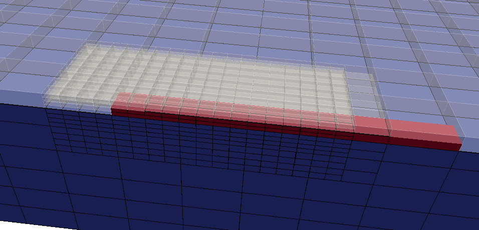
(a) Mesh of the thermal problem

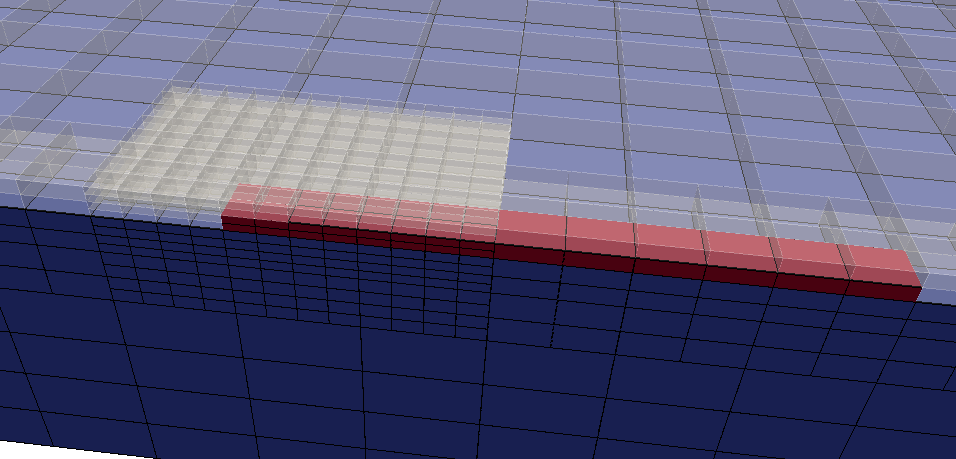
(b) Mesh of the mechanical problem

Figure 18: Meshes used for numerical simulation with material states, where red, blue and white (hollow) denote weld bead, plate and air, respectively.

Figure 18 shows a snapshot of the dynamic meshes of the thermal and the mechanical problems with material states, where red, blue and white (hollow) denote weld bead, plate and air, respectively. It should be noted that only the mechanical mesh is refined once along the welding line before deposition starts, which is not coarsened afterwards. Whereas, both meshes are dynamically refined twice towards the weld torch when material is deposited. The weld torch is set to travel 1.5 mm in each time step. Therefore, the newly deposited domain near the weld torch can be captured by the sub-element boundaries and the multi-level grid that keeps track of the physical domain. As the weld torch moves further away, these sub-elements are coarsened while the multi-level grid is used to remember the deposited domain as explained in Section 2.4 . Figure 19 depicts the dynamic meshes with temperature and longitudinal stress ($\sigma_{xx}$) distributions during the deposition period.

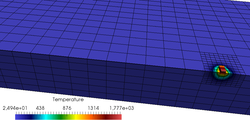
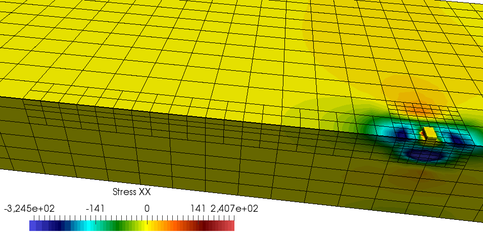
(a) t = 1 second

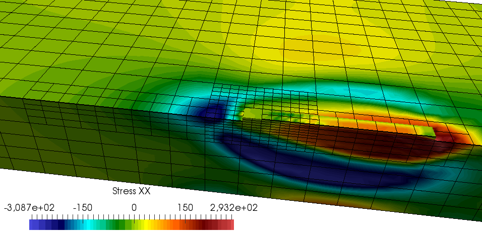
(b) t = 5.1 seconds

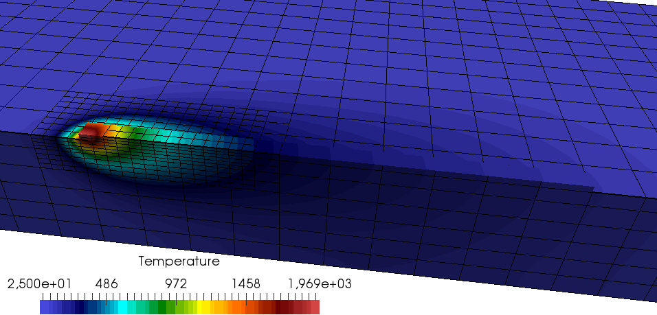
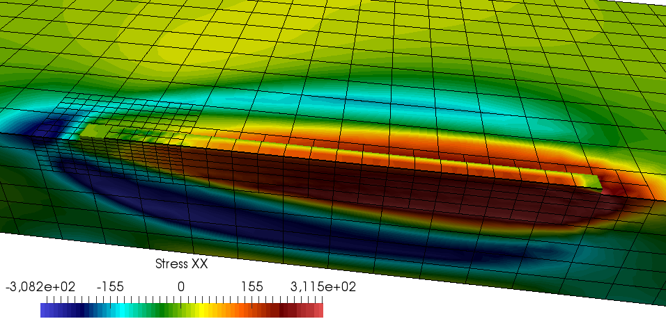
(c) t = 13.2 seconds

Figure 19: Evolution of the temperature and longitudinal stress longitudinal stress ($\sigma_{xx}$) distributions during the welding process on dynamic meshes at various time states.

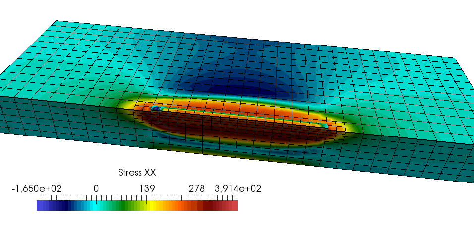
(a) Longitudinal stresses ($\sigma_{xx}$)

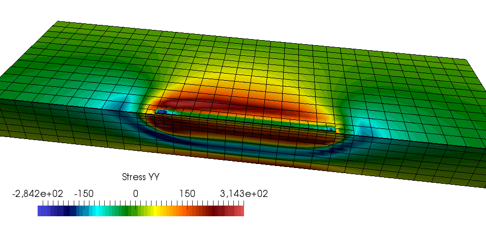
(b) Transverse stresses ($\sigma_{yy}$)

Figure 20: Residual stress distributions after cooling down to room temperature.

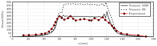
(a) Longitudinal stresses ($\sigma_{xx}$)

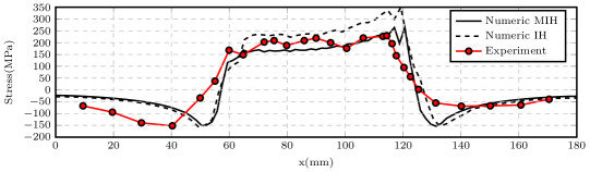
(b) Transverse stresses ($\sigma_{yy}$)

Figure 21: Numerical and experimental ([45]) results over line AB (IH: Isotropic hardening, MIH: Modified isotropic hardening)

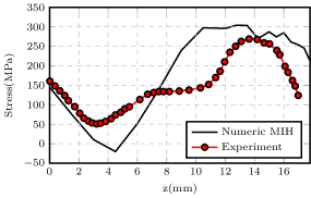
(a) Longitudinal stresses ($\sigma_{xx}$)

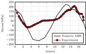
(b) Transverse stresses ($\sigma_{yy}$)

Figure 22: Numerical and experimental ([45]) results over line CD (MIH: Modified isotropic hardening)

Residual stress distributions after the parts are cooled down to the room temperature are given in Figure 20 over the physical domain. Gilles et. al. [45] measures the longitudinal and transverse residual stresses with a neutron diffraction technique over the lines AB and CD. These lines can be seen in Figure 17 . Figure 21 and Figure 22 compare the numerically predicted residual stresses to the measurements from experiment by Gilles et. al. along the lines AB and CD, respectively. It can be seen from these figures that the measured and the numerically computed stress profiles are in good agreement. However, utilizing the complete isotropic hardening values in Table 2 results in higher residual stress especially for the longitudinal stress component, which is also reported by Gilles et. al. [45]. Their explanation for effect is that the isotropic hardening law which does not consider stress relaxation due to viscoplastic effects or hardening recovery is not good enough to simulate cyclic loads which occur during the welding process. Therefore, the isotropic hardening model is modified in this work such that over one percent of plastic strain the material is assumed to behave elastic perfectly plastic. The results with this modified model match the experimental values as illustrated in Figure 21.

4 Summary and conclusions

The article at hand evaluates if high-order finite elements may be used in metal deposition modeling. To this end, the finite cell method, an embedded domain method of high order, was used. It was demonstrated that this method, combined with the multi-level $hp$-method, leads to high-order convergence rates even if neither, the physical boundaries nor the plastic front is resolved by the boundaries of the computational mesh. Therefore, high-order embedded domain modeling is a valid computational option. Very accurate results were also achieved in the thermo-elasto-plastic setting. Therein, the thermal and the elasto-plastic field variables were computed on their own high-order discetizations and coupled by means of a classical staggered scheme. In all of the computations the state variables were decoupled from the finite cells in an FCM sense by managing them on another computational grid. This allows for their separate coarsening and refinement and a simulation where material can be submerged into the computation on a sub-element level i.e. the addition of material is not equal to the addition of finite cells. The methods were thoroughly verified in semi-analytical benchmarks and then applied to an experimental benchmark of metal deposition. A good agreement with the experimentally measured residual strains/stresses was found.

While the overall computational methodology leads to very accurate results open research questions remain. For example, the presented de-refinements in the mechanical part of the simulation are clearly a valid option to accurately compute the stress states in the vicinity of a plastic front. However, the stress state in a manufactured part does not only consist of one plastic front and rather smooth stress states to the side of it. Instead, very complex, local stress states may be present. A straightforward coarsening procedure of the grid in these regions will cause smoothing effects for variables which are not diffusive by nature. It is beyond the scope of this paper to study the influence of strong, local coarsening in complex stress states and their effect in more involved computations. The investigation of this challenge remains open. Since the local plastic strains are not connected to the finite cells but stored in an extra grid which acts like a computational database, one option would be not to coarsen them at all. The computational grid, carrying the degrees of freedom could be coarsened independently. Such a procedure would allow for a constant number of degrees of freedom throughout the computation while detailed information on the local plastic strains would still be available if needed even if the finite cells were coarsened.

Next, it is worthwile to investigate the wall-clock time advantages of the computational approach w.r.t. conventional modeling techniques in detail. This is not easy to some extent because a fair comparison requires an efficient implementation of both techniques which is not available at present. Clearly, the modeling flexibility gained by the presented embedded domain method of high order using transient refinements does introduce a certain implementational as well as a computational overhead as compared to a classical fixed-grid approaches. The break-even point of refining and de-refining regarding wall-clock time further depends on the scale of the computations. However, to refine everywhere to the finest level required locally is also not an option. Thus, refinements and de-refinements must be used for efficient computations. How this is possible was investigated in the article at hand, but its comparison to other refinement techniques remains an open question. The current computations hint that the type of microscopic computations in the metal depositing process presented in the last example pay off in a multi-layer process whereby the refinement and de-refinement is not carried out at each time increment.

In summary, the article presents the first verified and validated steps of a novel computational methodology for the analysis of metal deposition modeling in an embedded domain sense using locally refined, transient discretizations of $hp$-type. As such, it demonstrates that this computational methodology is a valid option for the analysis of metal deposition.

References

References

- [1] J. A. Goldak, M. Akhlaghi, Computational Welding Mechanics, Springer, New York, 2005.
- [2] L. E. Lindgren, L.E. Lindgren-Computational Welding Mechanics Thermomechanical and Microstructural Simulations, Woodhead Publishing Limited and CRC Press LLC, 2007.
- [3] M. Tanaka, An introduction to physical phenomena in arc welding processes, Welding International 18 (11) (2004) 845–851. doi:10.1533/wint.2004.3342.
- [4] O. Zinovieva, A. Zinoviev, V. Ploshikhin, Three-dimensional modeling of the microstructure evolution during metal additive manufacturing, Computational Materials Science 141 (2018) 207–220. doi:10.1016/j.commatsci.2017.09.018.
- [5] A. Basak, S. Das, Epitaxy and Microstructure Evolution in Metal Additive Manufacturing, Annual Review of Materials Research 46 (1) (2016) 125–149. doi:10.1146/annurev-matsci-070115-031728.
- [6] C. Körner, Additive manufacturing of metallic components by selective electron beam melting — a review, International Materials Reviews 61 (5) (2016) 361–377. doi:10.1080/09506608.2016.1176289.
- [7] L. E. Lindgren, Numerical modelling of welding, Computer Methods in Applied Mechanics and Engineering 195 (48–49) (2006) 6710–6736, 00127. doi:10.1016/j.cma.2005.08.018.
- [8] L. E. Lindgren, H. A. Häggblad, J. M. J. McDill, A. S. Oddy, Automatic remeshing for three-dimensional finite element simulation of welding, Computer Methods in Applied Mechanics and Engineering 147 (3–4) (1997) 401–409, 00052. doi:10.1016/S0045-7825(97)00025-X.
- [9] B. Schoinochoritis, D. Chantzis, K. Salonitis, Simulation of metallic powder bed additive manufacturing processes with the finite element method: A critical review, Proceedings of the Institution of Mechanical Engineers, Part B: Journal of Engineering Manufacture 231 (1) (2017) 96–117. doi:10.1177/0954405414567522.
- [10] V. Nübel, A. Düster, E. Rank, An rp-adaptive finite element method for the deformation theory of plasticity, Computational Mechanics 39 (5) (2007) 557–574. doi:10.1007/s00466-006-0111-4.
- [11] M. Olesky, W. Cecot, Application of the fully automatic hp-adaptive FEM to elastic-plastic problems, Computer Methods in Materials Science 15 (1) (2015) 204–2012.
- [12] T. Elguedj, T. Hughes, Isogeometric analysis of nearly incompressible large strain plasticity, Computer Methods in Applied Mechanics and Engineering 268 (2014) 388–416. doi:10.1016/j.cma.2013.09.024.
- [13] A. Abedian, J. Parvizian, A. Düster, E. Rank, Finite cell method compared to h-version finite element method for elasto-plastic problems, Applied Mathematics and Mechanics 35 (10) (2014) 1239–1248, 00002. doi:10.1007/s10483-014-1861-9.
- [14] A. Taghipour, Parvizian, J., S. Heinze, A. Düster, The finite cell method for nearly incompressible finite strain plasticity problems with complex geometries, Computers & Mathematics with Applications (2018) accepted.
- [15] A. Düster, J. Parvizian, Z. Yang, E. Rank, The finite cell method for three-dimensional problems of solid mechanics, Computer Methods in Applied Mechanics and Engineering 197 (45–48) (2008) 3768–3782. doi:10.1016/j.cma.2008.02.036.
- [16] N. Zander, T. Bog, M. Elhaddad, F. Frischmann, S. Kollmannsberger, E. Rank, The multi-level hp-method for three-dimensional problems: Dynamically changing high-order mesh refinement with arbitrary hanging nodes, Computer Methods in Applied Mechanics and Engineering 310 (2016) 252–277. doi:10.1016/j.cma.2016.07.007.
- [17] N. Zander, T. Bog, S. Kollmannsberger, D. Schillinger, E. Rank, Multi-level hp-adaptivity: High-order mesh adaptivity without the difficulties of constraining hanging nodes, Computational Mechanics 55 (3) (2015) 499–517. doi:10.1007/s00466-014-1118-x.
- [18] J. Parvizian, A. Düster, E. Rank, Finite cell method, Computational Mechanics 41 (1) (2007) 121–133. doi:10.1007/s00466-007-0173-y.
- [19] A. Düster, E. Rank, B. A. Szabó, The p-version of the finite element method and finite cell methods, in: E. Stein, R. Borst, T. J. R. Hughes (Eds.), Encyclopedia of Computational Mechanics, Vol. 2, John Wiley & Sons, Chichester, West Sussex, 2017, pp. 1–35.
- [20] A. Abedian, J. Parvizian, A. Düster, E. Rank, The finite cell method for the J2 flow theory of plasticity, Finite Elements in Analysis and Design 69 (2013) 37–47, 00000. doi:10.1016/j.finel.2013.01.006.
- [21] E. de Souza Neto, P. Perić, P. Owen, Computational Methods for Plasticity: Theory and Applications, John Wiley & Sons, 2009.
- [22] D. Perić, C. Hochard, M. Dutko, D. R. J. Owen, Transfer operators for evolving meshes in small strain elasto-placticity, Computer Methods in Applied Mechanics and Engineering 137 (3) (1996) 331–344. doi:10.1016/S0045-7825(96)01070-5.
- [23] M. Ortiz, J. J. Quigley, Adaptive mesh refinement in strain localization problems, Computer Methods in Applied Mechanics and Engineering 90 (1) (1991) 781–804. doi:10.1016/0045-7825(91)90184-8.
- [24] N.-S. Lee, K.-J. Bathe, Error indicators and adaptive remeshing in large deformation finite element analysis, Finite Elements in Analysis and Design 16 (2) (1994) 99–139. doi:10.1016/0168-874X(94)90044-2.
- [25] O. C. Zienkiewicz, J. Z. Zhu, The superconvergent patch recovery and a posteriori error estimates. Part 2: Error estimates and adaptivity, International Journal for Numerical Methods in Engineering 33 (7) (1992) 1365–1382. doi:10.1002/nme.1620330703.
- [26] O. Zienkiewicz, J. Zhu, The superconvergent patch recovery (SPR) and adaptive finite element refinement, Computer Methods in Applied Mechanics and Engineering 101 (1-3) (1992) 207–224. doi:10.1016/0045-7825(92)90023-D.
- [27] B. Boroomand, O. C. Zienkiewicz, Recovery procedures in error estimation and adaptivity. Part II: Adaptivity in nonlinear problems of elasto-plasticity behaviour, Computer Methods in Applied Mechanics and Engineering 176 (1) (1999) 127–146. doi:10.1016/S0045-7825(98)00333-8.
- [28] A. R. Khoei, S. A. Gharehbaghi, Three-dimensional data transfer operators in large plasticity deformations using modified-SPR technique, Applied Mathematical Modelling 33 (7) (2009) 3269–3285. doi:10.1016/j.apm.2008.10.033.
- [29] A. Düster, H. Bröker, E. Rank, The p-version of the finite element method for three-dimensional curved thin walled structures, International Journal for Numerical Methods in Engineering 52 (7) (2001) 673–703.
- [30] D. Celentano, E. Oñate, S. Oller, A temperature-based formulation for finite element analysis of generalized phase-change problems, International Journal for Numerical Methods in Engineering 37 (20) (1994) 3441–3465.
- [31] S. Kollmannsberger, A. I. Özcan, E. Rank, Computational modeling of the SLM process: A hierarchical treatment of the transient heat equation with phase changes in preparation.
- [32] R. Hill, The Mathematical Theory of Plasticity, Oxford Classic Texts in the Physical Sciences, Oxford University Press, Oxford, New York, 1998.
- [33] L. Kudela, N. Zander, S. Kollmannsberger, E. Rank, Smart octrees: Accurately integrating discontinuous functions in 3D, Computer Methods in Applied Mechanics and Engineering 306 (Supplement C) (2016) 406–426, 00021. doi:10.1016/j.cma.2016.04.006.
- [34] H. Weber, B. Riemann, Die Partiellen Differential-Gleichungen Der Mathematischen Physik: Nach Riemann’s Vorlesungen in 5. Aufl. Bearb, no. v. 1, F. Vieweg und Sohn, 1912.
- [35] H. Hu, S. A. Argyropoulos, Mathematical modelling of solidification and melting: A review, Modelling and Simulation in Materials Science and Engineering 4 (4) (1996) 371.
- [36] D. W. Hahn, Heat Conduction, 3rd Edition, Wiley, Hoboken, N.J, 2012.
- [37] J. H. Weiner, B. A. Boley, Elasto-plastic thermal stresses in a solidifying body, Journal of the Mechanics and Physics of Solids 11 (3) (1963) 145–154, 00124.
- [38] C. E. Truman, M. C. Smith, The NeT residual stress measurement and modelling round robin on a single weld bead-on-plate specimen, International Journal of Pressure Vessels and Piping 86 (1) (2009) 1–2. doi:10.1016/j.ijpvp.2008.11.018.
- [39] C. Ohms, R. C. Wimpory, D. E. Katsareas, A. G. Youtsos, NET TG1: Residual stress assessment by neutron diffraction and finite element modeling on a single bead weld on a steel plate, International Journal of Pressure Vessels and Piping 86 (1) (2009) 63–72. doi:10.1016/j.ijpvp.2008.11.009.
- [40] X. Ficquet, D. J. Smith, C. E. Truman, E. J. Kingston, R. J. Dennis, Measurement and prediction of residual stress in a bead-on-plate weld benchmark specimen, International Journal of Pressure Vessels and Piping 86 (1) (2009) 20–30. doi:10.1016/j.ijpvp.2008.11.008.
- [41] M. Hofmann, R. C. Wimpory, NET TG1: Residual stress analysis on a single bead weld on a steel plate using neutron diffraction at the new engineering instrument ‘STRESS-SPEC’, International Journal of Pressure Vessels and Piping 86 (1) (2009) 122–125. doi:10.1016/j.ijpvp.2008.11.007.
- [42] S. Pratihar, M. Turski, L. Edwards, P. J. Bouchard, Neutron diffraction residual stress measurements in a 316L stainless steel bead-on-plate weld specimen, International Journal of Pressure Vessels and Piping 86 (1) (2009) 13–19. doi:10.1016/j.ijpvp.2008.11.010.
- [43] M. Turski, L. Edwards, Residual stress measurement of a 316l stainless steel bead-on-plate specimen utilising the contour method, International Journal of Pressure Vessels and Piping 86 (1) (2009) 126–131. doi:10.1016/j.ijpvp.2008.11.020.
- [44] X. Shan, C. M. Davies, T. Wangsdan, N. P. O’Dowd, K. M. Nikbin, Thermo-mechanical modelling of a single-bead-on-plate weld using the finite element method, International Journal of Pressure Vessels and Piping 86 (1) (2009) 110–121. doi:10.1016/j.ijpvp.2008.11.005.
- [45] P. Gilles, W. El-Ahmar, J.-F. Jullien, Robustness analyses of numerical simulation of fusion welding NeT-TG1 application: “Single weld-bead-on-plate”, International Journal of Pressure Vessels and Piping 86 (1) (2009) 3–12. doi:10.1016/j.ijpvp.2008.11.012.
- [46] S. K. Bate, R. Charles, A. Warren, Finite element analysis of a single bead-on-plate specimen using SYSWELD, International Journal of Pressure Vessels and Piping 86 (1) (2009) 73–78. doi:10.1016/j.ijpvp.2008.11.006.
- [47] P. J. Bouchard, The NeT bead-on-plate benchmark for weld residual stress simulation, International Journal of Pressure Vessels and Piping 86 (1) (2009) 31–42. doi:10.1016/j.ijpvp.2008.11.019.
- [48] M. C. Smith, A. C. Smith, NeT bead-on-plate round robin: Comparison of transient thermal predictions and measurements, International Journal of Pressure Vessels and Piping 86 (1) (2009) 96–109. doi:10.1016/j.ijpvp.2008.11.016.
- [49] J. Goldak, A. Chakravarti, M. Bibby, A new finite element model for welding heat sources, Metallurgical Transactions B 15 (2) (1984) 299–305. doi:10.1007/BF02667333.