Asymmetric pattern formation in microswimmer suspensions induced by orienting fields

Abstract

This paper studies the influence of orienting external fields on pattern formation, particularly mesoscale turbulence, in microswimmer suspensions. To this end, we apply a hydrodynamic theory that can be derived from a microscopic microswimmer model [H. Reinken et al., Phys. Rev. E 97, 022613 (2018)]. The theory combines a dynamic equation for the polar order parameter with a modified Stokes equation for the solvent flow. Here, we extend the model by including an external field that exerts an aligning torque on the swimmers (mimicking the situation in chemo-, photo-, magneto- or gravitaxis). Compared to the field-free case, the external field breaks the rotational symmetry of the vortex dynamics and leads instead to strongly asymmetric, traveling stripe patterns, as demonstrated by numerical solution and linear stability analysis. We further analyze the emerging structures using a reduced model which involves only an (effective) microswimmer velocity field. This model is significantly easier to handle analytically, but still preserves the main features of the asymmetric pattern formation. We observe an underlying transition between a square vortex lattice and a traveling stripe pattern. These structures can be well described in the framework of weakly nonlinear analysis, provided the strength of nonlinear advection is sufficiently weak.

Keywords: active matter, microswimmers, pattern formation, mesoscale turbulence, weakly nonlinear analysis

1 Introduction

Active matter exhibits a variety of large-scale self-organized structures that arise due to the interactions between the moving constituents. As shown in experiments, these structures are ranging from dynamical clustering [1, 2] and giant number fluctuations [3] to vortices and swirling [4, 5, 6]. To describe and understand the fascinating collective behavior from a theoretical point of view, models on different levels of detail have been applied, from studies simulating large numbers of individual particles [7, 8] to phenomenological approaches [9, 10, 11, 12, 13, 14] standing on the opposite side of the spectrum. To bridge the gap, many efforts have been made to derive coarse-grained hydrodynamic theories from microscopic models [15, 16, 17, 18, 19]. For a selection of recent reviews on the full scope of active matter see [20, 21, 22, 23, 24, 25, 26, 27, 28].

While many of the self-organized structures in systems of active constituents are well understood, the impact of external fields on the spatio-temporal pattern formation is mostly unexplored. For example, the motion of biological microswimmers such as bacteria or algae cells, is strongly determined by the response to external stimuli. These stimuli are of various origins: For example, swimmers react to concentration gradients (chemotaxis) [29, 30], a light source (phototaxis) [31, 32] or magnetic and gravitational fields (magnetotaxis [33, 34, 35, 36] and gravitaxis [37, 38]). The interplay between externally applied fields and internally generated motion is not only interesting from a fundamental perspective, but also essential for a variety of potential applications. For example, external fields offer the possibility to control the suspension in order to exploit the coherent motion of the swimmers. This includes tasks like cargo-delivery [39, 40, 41] (e.g., drug transport for medical purposes [42, 43]), powering microfluidic devices [44, 45] or swimmer-induced mixing on the small scales, where high Reynolds numbers are not accessible [46].

In the present paper, we explore the impact of an external field on a prominent example of active pattern formation, labeled and known as mesoscale turbulence [47]. This state can be observed in a variety of systems, including bacterial suspensions [48, 49, 50, 51] and Janus particles [52]. Mesoscale turbulence is characterized by chaotic vortex structures similar to inertial turbulence occurring in passive fluids at high Reynolds numbers [53], but it has two very unique features: First, it arises in the low Reynolds number regime of bacterial swimming (Stokes flow). Second, in contrast to inertial turbulence, it does not exhibit a spectrum of length scales but displays one characteristic vortex size controlled by the microswimmer details [50, 47, 54].

From the theoretical side, the main features of mesoscale turbulence have been successfully reproduced by a phenomenological continuum theory for the effective microswimmer velocity  [47, 55, 56, 57, 58, 59, 60, 61]. More recently, mesoscale turbulence and vortex lattices were also reported in a model of self-propelled particles with competing alignment interactions [62, 63]. Going beyond the purely phenomenological approach, we have recently presented a derivation of a hydrodynamic theory starting from Langevin equations for a generic microswimmer model [18, 19]. This theory consists of a dynamic equation for the polar order parameter field coupled to the solvent flow, the latter determined by a modified Stokes equation. In the limit of weak coupling between orientational order and solvent flow, our hydrodynamic theory reduces to the phenomenological model. Here, we extend the theory [19] towards the effect of an orienting external field, the aim being to describe situations where swimmers are subject to an externally applied torque (stemming, e.g., from a magnetic or gravitational field). To this end, we incorporate the field in the Langevin model and derive the additional terms in the dynamic equation for the polar order parameter. This is outlined in section 2 (and A) of the paper.

The remainder of the paper separates into two main parts. In the first part, we investigate the impact of an orienting external field in the full model consisting of the polar order parameter dynamics and an explicit equation for the solvent flow (i.e., a modified Stokes equation). Corresponding numerical results are presented in section 3. We show that, at intermediate field strengths, the emerging patterns become strongly asymmetric as a consequence of the externally broken symmetry. Performing a linear stability analysis (section 4), we find that this is due to the suppression of modes that are perpendicular to the field. For even higher external fields, the mesoscale-turbulent state is completely suppressed and we observe a homogeneous stationary polar state. The analytical results are then used to construct a state diagram of the system.

In the second part of the paper (section 5), we switch to a reduced model equivalent to the phenomenological theory, where the only dynamical variable is the effective microswimmer velocity field. The reduced model is significantly easier to handle analytically, but still exhibits the emergence of asymmetric patterns. Using the framework of weakly nonlinear analysis, we investigate the underlying transition from a square vortex lattice to a traveling stripe pattern that occurs upon an increase of the external field. Finally, we present conclusions and an outlook in section 6. The paper is supplemented by seven appendices providing technical details of the calculation.

2 Hydrodynamic theory

Recently, a phenomenological model [47, 55, 56, 57, 58, 59, 60, 61] has been proposed that reproduces the main features of mesoscale turbulence including the emergence of a characteristic length scale, i.e., vortex size [49]. It is a fourth-order field theory for the divergence-free collective microswimmer velocity and combines the Toner-Tu equation [64] with Swift-Hohenberg-like pattern formation. The main feature of the Toner-Tu equation is the transition from a disordered to a polar state corresponding to collective movement of the swimmers. Higher order gradient terms, as introduced in the Swift-Hohenberg equation, lead to a finite wavelength instability that is responsible for the collective length scale.

In earlier publications [18, 19] we have shown that an equivalent hydrodynamic theory for the microswimmer velocity can be derived via a Fokker-Planck equation approach starting from a generic Langevin model (similar to [15, 16]) for a system of microswimmers of length $\ell$, diameter $d$ and self-swimming speed $v_{0}$ with constant density $\rho$ (see A for a summary of the derivation). The Langevin model includes two types of interactions: First, there are short-range contributions stemming from an activity-driven polar interaction characterized by strength $\gamma_{0}$ and range $r$ [65]. Second, far-field hydrodynamic effects are included via a coupling to the solvent flow field $\mathbf{u}$. The latter is determined via an averaged Stokes equation supplemented by an appropriate ansatz for the active stress tensor containing gradient terms of up to fourth order. The resulting coarse-grained dynamics is then given by an equation for the polar order parameter field $\mathbf{P}$ (characterizing the swimmer’s mean local orientation) coupled to the solvent flow field $\mathbf{u}$. The effective velocity of the microswimmers is calculated as the sum $v_{0}\mathbf{P}+\mathbf{u}$. In the limit of weak coupling between the solvent flow and the polar order, the dependence on $\mathbf{u}$ can be neglected and the dynamics is adequately described by one field [19]. In contrast to the phenomenological approach, the coefficients of the field equation are directly linked to the parameters of the microscopic Langevin model [19] (see also A).

For the first part of this article, however, we will consider the full model consisting of both the dynamics of the polar order parameter $\mathbf{P}$ and the solvent flow $\mathbf{u}$. The dynamical equation for $\mathbf{P}(\mathbf{x},t)$ can be conveniently written in potential form

$$\mathfrak{D}_{t}(\mathbf{u})\mathbf{P}+\lambda_{0}\mathbf{P}\cdot\nabla\mathbf{P}=-\frac{\delta\mathfrak{F}}{\delta\mathbf{P}},\qquad\nabla\cdot\mathbf{P}=0.$$ (1)

The relaxation term is given as functional derivative of

$$\mathfrak{F}=q(\nabla\cdot\mathbf{P})+\frac{1}{2}\alpha|\mathbf{P}|^{2}+\frac{1}{4}\beta|\mathbf{P}|^{4}+\frac{1}{2}\Gamma_{2}(\nabla\mathbf{P})^{2}+\frac{1}{2}\Gamma_{4}(\nabla\nabla\mathbf{P})^{2}.$$ (2)

The derived equations (1) and (2) exhibit the same features as the phenomenological model: The isotropic–polar transition occurs when $\alpha$ changes sign from positive to negative. The coefficient $\beta$ of the cubic term determines the saturated value of the polar solution $\sqrt{-\alpha/\beta}$. For sufficiently strong activity $\Gamma_{2}$ becomes negative, which leads to a finite-wavelength instability of the homogeneous state, yielding a typical length scale of $\Lambda=2\pi\sqrt{-2\Gamma_{4}/\Gamma_{2}}$. Turbulent dynamics is introduced to the model via the nonlinear advection term on the left-hand side of equation (1), with $\lambda_{0}$ giving the strength of the advection term. Finally, $q(\mathbf{x})$ is a local Lagrange multiplier enforcing the incompressibility condition $\nabla\cdot\mathbf{P}=0$. The assumption of incompressibility is well suited for dense suspensions where density fluctuations become small [47].

In contrast to the phenomenological model, the solvent flow field $\mathbf{u}$ enters explicitly through the first term in equation (1). Its coupling to the polar order parameter field $\mathbf{P}$ is contained in the generalized derivative

$$\mathfrak{D}_{t}(\mathbf{u})\mathbf{P}=\partial_{t}\mathbf{P}+\mathbf{u}\cdot\nabla\mathbf{P}-\mathbf{\Omega}\cdot\mathbf{P}-\kappa\mathbf{\Sigma}\cdot\mathbf{P},$$ (3)

where the vorticity tensor and the deformation rate are given by $\mathbf{\Omega}=\frac{1}{2}\big{[}(\nabla\mathbf{u})^{\mathrm{T}}-(\nabla\mathbf{u})\big{]}$ and $\mathbf{\Sigma}=\frac{1}{2}\big{[}(\nabla\mathbf{u})^{\mathrm{T}}+(\nabla\mathbf{u})\big{]}$, respectively. The modified Stokes equation (see [19]) that determines the solvent flow field $\mathbf{u}$ reads

$$\nabla^{2}\mathbf{u}=c_{\mathrm{F}}\bigg{(}6c_{\mathrm{I}}\mathbf{P}\cdot\nabla\mathbf{P}+\nabla^{2}\mathbf{P}+\frac{1}{28}\nabla^{4}\mathbf{P}\bigg{)}+\nabla p,$$ (4)

where $p$ is an effective pressure, and the gradient terms of $\mathbf{P}$ stem from an expansion of the active stress.

Equations (1) to (4) are rescaled using the microswimmer length $\ell$ as length scale, the self-swimming speed $v_{0}$ as characteristic velocity and $\ell/v_{0}$ as time scale [19]. The coefficients can then be written as

$$\eqalign{\lambda_{0}=c_{\mathrm{I}}(3+2a_{0}P_{\mathrm{r}}c_{\mathrm{F}})/5,\qquad\kappa=a_{0}(3-c_{\mathrm{I}})/5,\\ \alpha=\left(1-c_{\mathrm{I}}\right)/P_{\mathrm{r}},\qquad\beta=\frac{3}{5}c_{\mathrm{I}}^{2}/P_{\mathrm{r}},\\ \Gamma_{2}=\frac{1}{10}\left(\frac{r}{\ell}\right)^{2}c_{\mathrm{I}}/P_{\mathrm{r}}-\frac{a_{0}}{15}P_{\mathrm{r}}c_{\mathrm{F}},\qquad\Gamma_{4}=-\frac{a_{0}}{420}P_{\mathrm{r}}c_{\mathrm{F}},}$$ (5)

where $P_{\mathrm{r}}$, $c_{\mathrm{I}}$, $r/\ell$, $c_{\mathrm{F}}$ and $a_{0}$ are dimensionless parameters. The activity is quantified by the persistence number $P_{\mathrm{r}}=v_{0}\tau/\ell$, giving the swimming speed compared to the reorientation time $\tau$. The strength and range of the polar interaction are given by $c_{\mathrm{I}}$ and $r/\ell$, respectively. For $c_{\mathrm{I}}<1$ the system favors a disordered, isotropic state, while for $c_{\mathrm{I}}>1$ it favors an ordered, polar state. The coupling to the solvent flow is characterized by the coefficient $c_{\mathrm{F}}$. For the dependence of $c_{\mathrm{I}}$ and $c_{\mathrm{F}}$ on microscopic parameters of the microswimmer model, see A. Finally, flow aligning effects are characterized by the shape parameter $a_{0}$ which depends on the swimmer aspect ratio [see equation (30) in A].

In the present work, we extend equation (1) by terms incorporating an external field that affects the swimmer’s orientations. On the microscopic level, we assume that the external field generates a potential for every swimmer which depends on the angle between the field’s direction $\mathbf{h}$ and swimmer orientation $\mathbf{n}$ according to a standard ferromagnetic coupling, i.e., $\Phi_{\mathrm{ext}}\propto-\mathbf{n}\cdot\mathbf{h}$. This term also occurs in some passive liquids in an orienting field (e.g., ferrofluids [66, 67], which are suspensions of ferromagnetic colloids in a passive solvent) and was recently considered in the context of active fluids. Indeed, the same ansatz has been used to describe chemotactic [30] and magnetotactic [68] bacteria. It is in principle applicable to any microswimmer suspension subjected to an aligning torque exerted by an external field, as it occurs, e.g., in magnetotaxis [33, 34, 35, 36], phototaxis [31, 32] or gravitaxis [37, 38]. Introducing the external potential in the Langevin equations and performing the same steps as in the field-free case, one arrives at the order parameter equation (for details see A)

$$\mathfrak{D}_{t}(\mathbf{u})\mathbf{P}+\lambda_{0}\mathbf{P}\cdot\nabla\mathbf{P}=-\frac{\delta\mathfrak{F}}{\delta\mathbf{P}}+\mathbf{g},\qquad\nabla\cdot\mathbf{P}=0.$$ (6)

The additional term on the right-hand side of the evolution equation is given as

$$\mathbf{g}=B_{0}\mathbf{h}\cdot\bigg{[}\frac{2}{3}\mathbf{I}-\frac{3}{5}c_{\mathrm{I}}\bigg{(}\mathbf{P}\mathbf{P}-\frac{\mathbf{I}(\mathbf{P}\cdot\mathbf{P})}{3}\bigg{)}-\frac{2}{15}a_{0}P_{\mathrm{r}}\mathbf{\Sigma}\bigg{]},$$ (7)

where $B_{0}$ denotes the dimensionless external field strength. The first term on the right-hand side of equation (7) increases the polar order in the direction of the external field, similar to what happens in passive fluids. The second term arises due to the conservation of the unit vector $\mathbf{n}$, i.e., the microswimmer’s orientation. It leads to a saturation of $\mathbf{P}$ with increasing $B_{0}$, as we will later see (compare figure 2). Finally, the third term in equation (7) arises as a consequence of the closure scheme applied for the nematic order parameter tensor $\mathbf{Q}$ (see A). Clearly, this term incorporates a coupling to the solvent flow field. Physically, it adds a reduction of polar order due to the flows generated by the swimmers.

3 Numerical observations

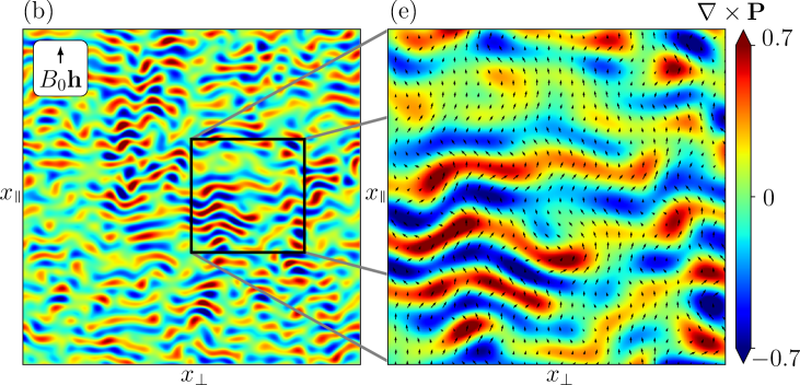
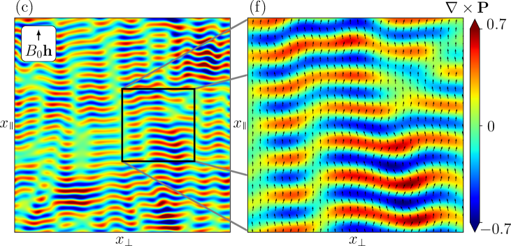
Figure 1: Snapshot of the (scalar) vorticity of the polar order parameter field as heatmap plot for (a) $B_{0}=0$, (b) $B_{0}=0.6$ and (c) $B_{0}=0.8$. Blue means clockwise, red counter-clockwise rotation. The enlarged versions (d),(e) and (f) visualize additionally the polar order parameter field by arrows, with the length corresponding to the magnitude of the field. The remaining parameters are $P_{\mathrm{r}}=8$, $c_{\mathrm{I}}=0.5$, $c_{\mathrm{F}}=0.1$, $r/\ell=1$ and $\ell/d=6$.

The aim of the present study is to explore the impact of a spatially homogeneous stationary field on the mesoscale-turbulent state observed in the absence of a field. As a starting point, we will discuss the dynamical behavior that can be observed based on numerical solution of equation (6) for the polar order parameter field $\mathbf{P}$, coupled to the Stokes equation (4) for the flow field $\mathbf{u}$. The solution is performed in two-dimensional space (for the numerical methods, see B).

We start with the field-free case, $B_{0}=0$. Here, we focus on parameters where the system is in a mesoscale turbulent state. In figure 1(a) a snapshot of the (scalar) vorticity of the polar order parameter field is shown. For a more descriptive visualization of the dynamics in the absence of a field see the supplementary movie 1. For better visibility, a section of the field is presented in a larger version in figure 1(d). Here, we also visualize the (vectorial) order parameter field by arrows, with the arrow length indicating the magnitude of the polar order. The observed dynamical state is characterized by the formation, motion and decay of clockwise (blue) and counter-clockwise (red) rotating vortices. The emerging patterns are dominated by one characteristic length or vortex size depending on the microscopic parameters of the swimmers [50, 47, 54, 18, 19], hence the name mesoscale turbulence. This stands in contrast to inertial turbulence observed in the Navier–Stokes equation where one finds a broad spectrum of vortex sizes [53]. For a more detailed discussion on the turbulent state without the influence of external fields, see [47, 59, 58, 61] for the phenomenological model and [18, 19] for the present model. Note that, compared to most of the listed publications, the coefficient $\lambda_{0}$ is rather large and, therefore, the shape of the vortices is highly irregular.

Turning on the external field, $B_{0}>0$, introduces several new features. First, the external field induces a net polar order in the system, that is $\langle\mathbf{P}\rangle=A^{-1}\int\rmd\mathbf{x}\mathbf{P}(\mathbf{x},t)\neq 0$ (where $A$ is the area). The swimmer’s self-propulsion speed leads to a local transport in the direction of the polar order given by $v_{0}\mathbf{P}$. Thus, as a consequence of the generated net polar order, we observe a net transport in the direction of the field. Second, the overall rotational symmetry is broken, which leads to the emergence of asymmetric patterns. In figure 1(b) and (c) this is illustrated by snapshots of the vorticity at finite (nonzero) field strengths. In contrast to the case $B_{0}=0$, we here observe the formation of elongated structures in the vorticity field, or, more precisely, a highly irregular stripe pattern with numerous defects. In figure 1(c), where the field strength is larger compared to (b), the number of defects is smaller and the stripe pattern more regular. Interestingly, the defects are elongated in the direction parallel to the field. The enlarged sections in figure 1(e) and (f) additionally show the polar order in the field’s direction. For a visualization of the transport of the patterns, see the supplementary movies 2 and 3. They show the dynamics for the same values of the field strength as represented in figure 1(b) and (c), i.e. $B_{0}=0.6$ and $B_{0}=0.8$, respectively. In the remainder of this work we will elucidate the observed dynamical features using analytical methods, particularly linear stability analysis and weakly nonlinear analysis.

4 Analytical construction of the state diagram

4.1 Homogeneous stationary solution

If the activity is sufficiently weak or the external field sufficiently strong, we numerically observe a homogeneous stationary state. This state is the starting point of our linear stability analysis.

Clearly, the external field breaks the rotational symmetry of the system. Thus, it is useful to distinguish between components of the polarization parallel and perpendicular to the field, i.e., $\mathbf{P}=(P_{\mkern 4.0mu\vphantom{\perp}\vrule depth=0.0pt\mkern 3.0mu\vrule depth=0.0pt\mkern 5.0mu},P_{\perp})$. To calculate the homogeneous stationary solution, we assume a quiescent state, where the solvent velocity field vanishes, i.e., $\mathbf{u}=0$. Further, the pressure $p=p_{0}$ and Lagrange-multiplier $q=q_{0}$ are set constant in space and time. Then, equation (6) reduces to

$$0=-\alpha P_{0}-\beta P_{0}^{3}+\frac{2}{3}B_{0}-\frac{2}{5}B_{0}c_{\mathrm{I}}P_{0}^{2}.$$ (8)

The real positive solution of equation (8) defines the homogeneous stationary state $\mathbf{P}=(P_{0},0)$. This solution $P_{0}$ is plotted versus the external field strength $B_{0}$ in figure 2. As expected, the polar order grows upon increasing the field strength. Dividing by $B_{0}$ and evaluating the limit $B_{0}\to\infty$, equation (8) simplifies to

$$0=\frac{2}{3}-\frac{2}{5}c_{\mathrm{I}}P_{0}^{2}.$$ (9)

The solution of equation (9) defines the saturation value $P_{0}^{\mathrm{sat}}=\sqrt{5/(3c_{\mathrm{I}})}$ that is approached for $B_{0}\to\infty$.

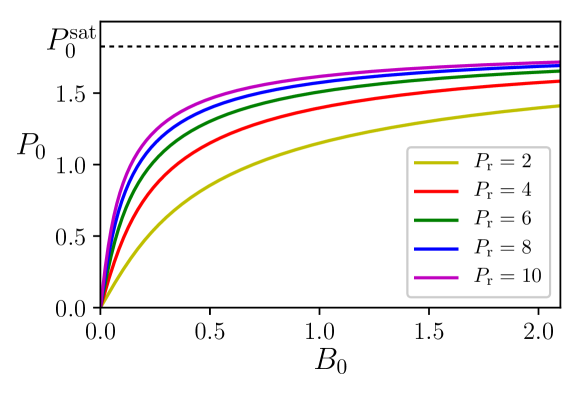
Figure 2: Homogeneous stationary solution $P_{0}$ as function of the external field strength $B_{0}$ for different values of the persistence number $P_{\mathrm{r}}$. The saturation value $P_{0}^{\mathrm{sat}}$ appearing for very large external field strength is independent of $P_{\mathrm{r}}$. The remaining parameter is $c_{\mathrm{I}}=0.5$.

4.2 Linear stability analysis

In order to determine the linear stability of the homogeneous stationary solution $\mathbf{P}=(P_{0},0)$, $q=q_{0}$, $\mathbf{u}=(0,0)$, $p=p_{0}$, we consider small perturbations, i.e.,

$$\eqalign{P_{\mkern 4.0mu\vphantom{\perp}\vrule depth=0.0pt\mkern 3.0mu\vrule depth=0.0pt\mkern 5.0mu}=P_{0}+\delta P_{\mkern 4.0mu\vphantom{\perp}\vrule depth=0.0pt\mkern 3.0mu\vrule depth=0.0pt\mkern 5.0mu},&P_{\perp}=\delta P_{\perp},\qquad q=q_{0}+\delta q,\\ u_{\mkern 4.0mu\vphantom{\perp}\vrule depth=0.0pt\mkern 3.0mu\vrule depth=0.0pt\mkern 5.0mu}=\delta u_{\mkern 4.0mu\vphantom{\perp}\vrule depth=0.0pt\mkern 3.0mu\vrule depth=0.0pt\mkern 5.0mu},&u_{\perp}=\delta u_{\perp},\qquad p=p_{0}+\delta p.}$$ (12)

For all perturbations, we make the ansatz

$$(\delta P_{\mkern 4.0mu\vphantom{\perp}\vrule depth=0.0pt\mkern 3.0mu\vrule depth=0.0pt\mkern 5.0mu},\delta P_{\perp},\delta q,\delta u_{\mkern 4.0mu\vphantom{\perp}\vrule depth=0.0pt\mkern 3.0mu\vrule depth=0.0pt\mkern 5.0mu},\delta u_{\perp},\delta p) =(\delta\hat{P}_{\mkern 4.0mu\vphantom{\perp}\vrule depth=0.0pt\mkern 3.0mu\vrule depth=0.0pt\mkern 5.0mu},\delta\hat{P}_{\perp},\delta\hat{q},\delta\hat{u}_{\mkern 4.0mu\vphantom{\perp}\vrule depth=0.0pt\mkern 3.0mu\vrule depth=0.0pt\mkern 5.0mu},\delta\hat{u}_{\perp},\delta\hat{p})\ \rme^{\sigma t+\rmi\mathbf{k}\cdot\mathbf{x}},$$ (13)

with wavevector $\mathbf{k}=(k_{\mkern 4.0mu\vphantom{\perp}\vrule depth=0.0pt\mkern 3.0mu\vrule depth=0.0pt\mkern 5.0mu},k_{\perp})$. We now insert equations (12) and (13) into equations (2), (3), (4), (6) and (7) and linearize with respect to the perturbations. As shown in C, the perturbations of the velocity field $\delta\mathbf{u}$, the pressure $\delta p$ and the Lagrange multiplier $\delta q$ can be related to the perturbations of the polar order parameter $\delta\mathbf{P}$. As a result (see C) one obtains a linearized system involving only $\delta\mathbf{P}$, that is

$$\sigma\delta\hat{\mathbf{P}}=\mathbf{\Pi}(\mathbf{k})\cdot\mathbf{M}(\mathbf{k})\cdot\delta\hat{\mathbf{P}},$$ (14)

where the projector $\mathbf{\Pi}(\mathbf{k})=\mathbf{I}-\mathbf{k}\mathbf{k}/|\mathbf{k}|^{2}$ arises as a consequence of the incompressibility of the order parameter field, and the $2\times 2$-matrix $\mathbf{M}(\mathbf{k})$ is the Jacobian. The components of $\mathbf{M}(\mathbf{k})$ are given in equation (C) in C. We obtain the complex growth rate $\sigma=\sigma_{\mathrm{Re}}+\rmi\sigma_{\mathrm{Im}}$ as a function of the wavevector $\mathbf{k}$ by calculating the eigenvalues of the matrix $\mathbf{\Pi}(\mathbf{k})\cdot\mathbf{M}(\mathbf{k})$. The real part $\sigma_{\mathrm{Re}}(\mathbf{k})$, which determines the actual growth of a mode $\mathbf{k}$, is given by

$$\sigma_{\mathrm{Re}}(\mathbf{k})= -\alpha-\Gamma_{2}|\mathbf{k}|^{2}-\Gamma_{4}|\mathbf{k}|^{4}-\beta P_{0}^{2}\Big{(}k_{\mkern 4.0mu\vphantom{\perp}\vrule depth=0.0pt\mkern 3.0mu\vrule depth=0.0pt\mkern 5.0mu}^{2}+3k_{\perp}^{2}\Big{)}/|\mathbf{k}|^{2}$$

$$+3c_{\mathrm{F}}c_{\mathrm{I}}P_{0}\Big{(}P_{0}(1+\kappa)-\frac{2}{15}a_{0}P_{\mathrm{r}}B_{0}\Big{)}k_{\mkern 4.0mu\vphantom{\perp}\vrule depth=0.0pt\mkern 3.0mu\vrule depth=0.0pt\mkern 5.0mu}^{2}/|\mathbf{k}|^{2}$$

$$-\frac{c_{\mathrm{I}}}{5}B_{0}P_{0}\Big{(}3k_{\mkern 4.0mu\vphantom{\perp}\vrule depth=0.0pt\mkern 3.0mu\vrule depth=0.0pt\mkern 5.0mu}^{2}+4k_{\perp}^{2}\Big{)}/|\mathbf{k}|^{2}.$$

The imaginary part $\sigma_{\mathrm{Im}}(\mathbf{k})$, which determines the linear traveling speed $c_{0}^{\mkern 4.0mu\vphantom{\perp}\vrule depth=0.0pt\mkern 3.0mu\vrule depth=0.0pt\mkern 5.0mu}$, is given by

$$\eqalign{\sigma_{\mathrm{Im}}(\mathbf{k})&=\Big{[}-\lambda_{0}P_{0}+\frac{c_{\mathrm{F}}}{2}\Big{(}P_{0}(1+\kappa)-\frac{2}{15}B_{0}a_{0}P_{\mathrm{r}}\Big{)}\Big{(}1-\frac{|\mathbf{k}|^{2}}{28}\Big{)}\Big{]}k_{\mkern 4.0mu\vphantom{\perp}\vrule depth=0.0pt\mkern 3.0mu\vrule depth=0.0pt\mkern 5.0mu}\\ &=-c_{0}^{\mkern 4.0mu\vphantom{\perp}\vrule depth=0.0pt\mkern 3.0mu\vrule depth=0.0pt\mkern 5.0mu}k_{\mkern 4.0mu\vphantom{\perp}\vrule depth=0.0pt\mkern 3.0mu\vrule depth=0.0pt\mkern 5.0mu}.}$$ (16)

It is seen that $\sigma_{\mathrm{Re}}(\mathbf{k})$ depends not only on the magnitude $|\mathbf{k}|=k$ of the wavevector but also on its direction. For $B_{0}=0$ and $c_{\mathrm{F}}=0$, one reproduces the growth rate obtained in [55].

4.3 State diagram

Due to the explicit dependence of the growth rate $\sigma_{\mathrm{Re}}(\mathbf{k})$ on the wavevector’s direction, it makes sense to distinguish between two limiting cases illustrated in figure 3: perturbations with a wavevector that is purely parallel to the external field, i.e., $k_{\mkern 4.0mu\vphantom{\perp}\vrule depth=0.0pt\mkern 3.0mu\vrule depth=0.0pt\mkern 5.0mu}=k$, $k_{\perp}=0$, or purely perpendicular to the field, i.e., $k_{\mkern 4.0mu\vphantom{\perp}\vrule depth=0.0pt\mkern 3.0mu\vrule depth=0.0pt\mkern 5.0mu}=0$, $k_{\perp}=k$. The incompressibility condition of the order parameter field, i.e., $k_{\mkern 4.0mu\vphantom{\perp}\vrule depth=0.0pt\mkern 3.0mu\vrule depth=0.0pt\mkern 5.0mu}\delta P_{\mkern 4.0mu\vphantom{\perp}\vrule depth=0.0pt\mkern 3.0mu\vrule depth=0.0pt\mkern 5.0mu}+k_{\perp}\delta P_{\perp}=0$, then dictates the form of the respective perturbations. For a parallel wavevector, the component $\delta P_{\mkern 4.0mu\vphantom{\perp}\vrule depth=0.0pt\mkern 3.0mu\vrule depth=0.0pt\mkern 5.0mu}$ must vanish. Therefore, the linearly unstable pattern is a perturbation in the perpendicular direction with periodicity in the parallel direction [see figure 3(a)]. The corresponding wavelength is given by $\Lambda_{\mkern 4.0mu\vphantom{\perp}\vrule depth=0.0pt\mkern 3.0mu\vrule depth=0.0pt\mkern 5.0mu}=2\pi/k$. This type of pattern manifests itself as stripes in the vorticity of the field. Analogously, for a perpendicular wavevector, the component $\delta P_{\perp}$ must vanish and the pattern is a perturbation along the field with periodicity in the perpendicular direction ($\Lambda_{\perp}=2\pi/k$) [see figure 3(b)]. The occurrence of both, modes in the parallel and in the perpendicular direction, results in a square vortex lattice.

Figure 3: Form of the perturbed polar order parameter field in the two limiting cases of a wavevector (a) parallel and (b) perpendicular to the external field. The corresponding dominating wavelength $\Lambda_{\mkern 4.0mu\vphantom{\perp}\vrule depth=0.0pt\mkern 3.0mu\vrule depth=0.0pt\mkern 5.0mu}$ or $\Lambda_{\perp}$, respectively, is indicated in red

Figure 4: (a) State diagram in the $P_{\mathrm{r}}$-$B_{0}$-plane obtained by linear stability analysis. (b) - (e) Real part of the growth rate as function of the wavenumber for $\mathbf{k}{\mkern 4.0mu\vphantom{\perp}\vrule depth=0.0pt\mkern 3.0mu\vrule depth=0.0pt\mkern 5.0mu}\mathbf{h}$ and $\mathbf{k}\perp\mathbf{h}$. The solid line in (a) denotes the field strength where parallel modes start to grow, the dashed line where perpendicular modes start to grow. The remaining parameters are $c_{\mathrm{I}}=0.5$, $r/\ell=1$, $c_{\mathrm{F}}=0.1$ and $\ell/d=6$. Note that the diagram is independent of the magnitude of the nonlinear advection term $\lambda_{0}$.

The results obtained from linear stability analysis and the distinction between the two limiting cases for the perturbation enable the construction of a state diagram in the plane spanned by $P_{\mathrm{r}}$ and $B_{0}$, see figure 4(a). The diagram is supplemented by plots of the growth rate as function of the wavevector, see figures 4(b) to (e). Regions where the homogeneous stationary state described in section 4.1 is stable are indicated by a white background color. Considering first the case $B_{0}=0$, we observe an instability at a critical value ($P_{\mathrm{r}}\approx 5$) where mesoscale turbulence sets in. This is reflected by a band of unstable modes (see figure 4(c)), one of which grows the fastest and yields a typical vortex size $\Lambda=2\pi\sqrt{-2\Gamma_{4}/\Gamma_{2}}$. Note that, without an external field, the full rotational symmetry is still intact and the two curves for parallel and perpendicular wavevector perturbations coincide. For a (numerical) snapshot of the order parameter field $\mathbf{P}$ and its vorticity $\nabla\times\mathbf{P}$ in the mesoscale turbulent state at $B_{0}=0$, see figure 1(a).

Keeping the persistence number at a constant value within the zero-field turbulent state, e.g., $P_{\mathrm{r}}=8$, and increasing the external field from zero results in a shift of the growth rate curve $\sigma_{\mathrm{R}}$ depending on the wavevector’s direction (see figure 4(d)). It is seen that perturbations with perpendicular wavevector become suppressed above a field strength of $B_{0}^{\perp}(P_{\mathrm{r}})$, see dashed line in figure 4(a). In contrast, perturbations with parallel wavevector still grow until a larger field strength of $B_{0}^{\mkern 4.0mu\vphantom{\perp}\vrule depth=0.0pt\mkern 3.0mu\vrule depth=0.0pt\mkern 5.0mu}(P_{\mathrm{r}})$ is reached, see solid line in figure 4(a). Between the two “critical” field strengths $B_{0}^{\mkern 4.0mu\vphantom{\perp}\vrule depth=0.0pt\mkern 3.0mu\vrule depth=0.0pt\mkern 5.0mu}$ and $B_{0}^{\perp}$, the growth of parallel modes leads to asymmetric patterns which are elongated in the perpendicular direction. This is consistent with our numerical observations shown in figure 1(b) and (c). Interestingly, the characteristic length given by the critical mode $k_{\mathrm{c}}$, i.e., the maximum of $\sigma_{\mathrm{Re}}(\mathbf{k})$, is not influenced by the external field [compare figure (4)(c) to (e)].

Moreover, we observe a very intriguing feature in the case of a perturbation with $\mathbf{k}{\mkern 4.0mu\vphantom{\perp}\vrule depth=0.0pt\mkern 3.0mu\vrule depth=0.0pt\mkern 5.0mu}\mathbf{h}$. Here, the growth rate curve is first shifted upwards for intermediate field strengths before being shifted down for stronger fields. This is due to the explicit coupling of the solvent flow to the generated polar order in the system. As discussed in a variety of publications [23, 9, 21], active suspensions with uniform orientational order such as active nematics [69] are intrinsically unstable. The interplay between actively generated flow and the resulting flow alignment of the elongated particles destabilizes the uniaxial order. In active nematics, this results in a bend instability for particles that generate an extensile active stress and a splay instability for particles that generate a contractile active stress [21]. In our model of polar microswimmers, a similar mechanism leads to the upwards shift of the growth rate curve of parallel modes for intermediate field strengths. The external field generates orientational order, which in turn induces a solvent flow that destabilizes the homogeneous state due to the flow alignment of the swimmers. For higher field strengths, however, this interplay between polar order and solvent flow is outweighed by the other terms in the growth rate [equation 4.2] that suppress the instability. This behavior is reflected in the state diagram in figure 4(b) by the pronounced “bulge” for persistence numbers below $P_{\mathrm{r}}\approx 5$.

Finally, note that the growth rate $\sigma_{\mathrm{Re}}$ [see equation (4.2)] does not depend on the nonlinear advection term in equation (1). The imaginary part $\sigma_{\mathrm{Im}}$, however, is strongly dependent on to the parameter $\lambda_{0}$ characterizing the magnitude of the advection term [see equation (16)]. Thus, in the framework of linear stability analysis, the influence of the nonlinear advection term is restricted to transporting the emerging patterns with a traveling speed of $c_{0}^{\mkern 4.0mu\vphantom{\perp}\vrule depth=0.0pt\mkern 3.0mu\vrule depth=0.0pt\mkern 5.0mu}$, given by equation (16), in the direction of the external field. Comparing the state diagram in figure 4 to the full numerical solution of equations (6) and (4), we find that the analytical calculations are consistent with the numerical results. They accurately predict the onset of the mesoscale-turbulent state, the complete suppression of the instability for high field strength and the region of asymmetric patterns for intermediate field strength (compare figure 1).

5 Reduced model

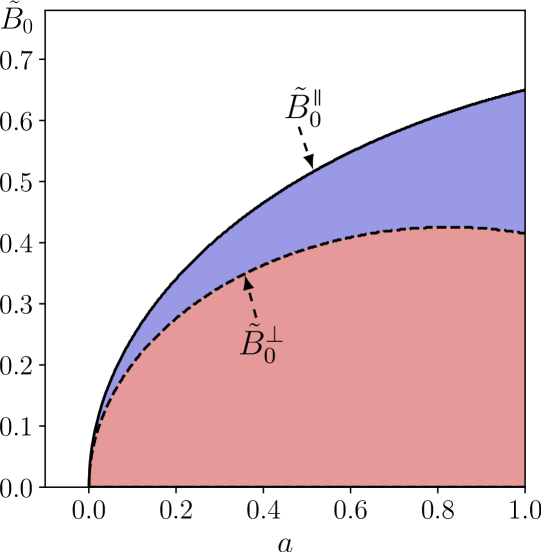
Figure 5: State diagram for the reduced model in the $a$-$\tilde{B}_{0}$-plane obtained by linear stability analysis. The solid line in the state diagram denotes the field strength where parallel modes start to grow, the dashed line where perpendicular modes start to grow. Compared to the state diagram of the full model (figure 4) the bulge for $P_{\mathrm{r}}<5$ which corresponds to $a<0$ is absent. The coefficient of the cubic term is set to $b=0.1$. Note that the diagram is independent of the magnitude of the nonlinear advection term $\lambda$.

In order to characterize the emergence of patterns in more detail, it seems appropriate to perform a weakly nonlinear analysis. However, it turns out that this is an extremely difficult task when starting from the model equations discussed so far. For the remainder of this work we thus consider a reduced model, which still gives the essential physics.

As we discussed in our previous publication [19], the response of the flow field to the forces exerted by every swimmer on the surrounding fluid scales with the coefficient $c_{\mathrm{F}}$. The latter is proportional to the ratio of active to viscous forces. In the limit $c_{\mathrm{F}}\ll 1$, the collective dynamics of the suspension depends solely on the dynamics of the polar order parameter. Introducing an effective microswimmer velocity proportional to $\mathbf{P}$ then reproduces the phenomenological model [47, 55, 56, 57, 58, 59, 61] briefly introduced in section 2, with the notable difference that we can calculate all the coefficients as functions of parameters of the microswimmer model. Note that the coefficient $\Gamma_{2}$ has to be negative in order to obtain a mesoscale-turbulent state. Thus, additionally to the limit $c_{\mathrm{F}}\ll 1$, the product $P_{\mathrm{r}}c_{\mathrm{F}}$ still has to be sufficiently large compared to $c_{\mathrm{I}}$ [see equation 5]. In this work, we rescale space and time by the length and time scale of the pattern formation, i.e., the inverse of the critical mode $k_{\mathrm{c}}=\sqrt{-\Gamma_{2}/(2\Gamma_{4})}$, and the inverse of the corresponding maximum of the growth rate $\sigma_{\mathrm{Re}}(\alpha=0,B_{0}=0)=\Gamma_{2}^{2}/(4\Gamma_{4})$. Further, we rescale by the saturation value for the polar order parameter at $B_{0}\to\infty$ and obtain the scaled collective microswimmer velocity via $\mathbf{v}=\mathbf{P}/P_{0}^{\mathrm{sat}}$, where $P_{0}^{\mathrm{sat}}=\sqrt{5/(3c_{\mathrm{I}})}$. The rescaled equation for $\mathbf{v}$ is then given by

$$\eqalign{\partial_{t}\mathbf{v}+\lambda\mathbf{v}\cdot\nabla\mathbf{v}=&-\nabla q+a\mathbf{v}-b|\mathbf{v}|^{2}\mathbf{v}-(1+\nabla^{2})^{2}\mathbf{v}\\ &+\tilde{B}_{0}\mathbf{h}\cdot\Big{[}\mathbf{I}-\frac{1}{2}\Big{(}3\mathbf{v}\mathbf{v}-\mathbf{I}(\mathbf{v}\cdot\mathbf{v})\Big{)}\Big{]}.}$$ (17)

The advantage of this scaling is that the number of independent coefficients is now reduced to four: First, the coefficient $\lambda$ determines the strength of the nonlinear advection term. Second, the coefficient $a$ characterizes the distance to the onset of the instability at $\tilde{B}_{0}=0$. For $a<0$, the system favors the isotropic homogeneous state, while for $a>0$ the system develops mesoscale turbulence. Note that for $a>1$, the homogeneous stationary solution becomes polar. In this work, we will focus on the case $a<1$. Third, the coefficient $b$ of the cubic term in $\mathbf{v}$ is responsible for the saturation of the emerging patterns. Fourth, the external field strength is given by $\tilde{B}_{0}$. The scaling of the Lagrange multiplier $q$ enforcing the incompressibility $\nabla\cdot\mathbf{v}=0$ is irrelevant, thus, we keep the same notation as before. For the explicit dependencies of the four remaining coefficients $\lambda$, $a$, $b$ and $\tilde{B}_{0}$ on the coefficients of the full model for the dynamics of $\mathbf{P}$ given in equations (6) and (7), see D.

The reduced and rescaled model is significantly easier to handle than the full version but still exhibits the emergence of asymmetric patterns due to the external field. The homogeneous stationary solution $\mathbf{v}=(v_{\mkern 4.0mu\vphantom{\perp}\vrule depth=0.0pt\mkern 3.0mu\vrule depth=0.0pt\mkern 5.0mu},v_{\perp})=(V_{0},0)$ of the reduced model is calculated via

$$0=(a-1)V_{0}-bV_{0}^{3}+\tilde{B}_{0}-\tilde{B}_{0}V_{0}^{2}.$$ (18)

Analogous to the full model, performing a linear stability analysis yields the complex growth rate with real part

$$\sigma_{\mathrm{Re}}(\mathbf{k})=a-1+2|\mathbf{k}|^{2}-|\mathbf{k}|^{4}-bV_{0}^{2}\frac{k_{\mkern 4.0mu\vphantom{\perp}\vrule depth=0.0pt\mkern 3.0mu\vrule depth=0.0pt\mkern 5.0mu}^{2}+3k_{\perp}^{2}}{|\mathbf{k}|^{2}}-\frac{1}{2}\tilde{B}_{0}V_{0}\frac{3k_{\mkern 4.0mu\vphantom{\perp}\vrule depth=0.0pt\mkern 3.0mu\vrule depth=0.0pt\mkern 5.0mu}^{2}+4k_{\perp}^{2}}{|\mathbf{k}|^{2}}.$$ (19)

Similar to the corresponding function $\sigma_{\mathrm{\mathbf{k}}}$ of the full model [compare equation (4.2)], equation (19) yields a finite-wavelength instability. Due to the present scaling, the critical mode is now given by $k_{\mathrm{c}}=1$. Further, we obtain the linear traveling speed as

$$c_{0}^{\mkern 4.0mu\vphantom{\perp}\vrule depth=0.0pt\mkern 3.0mu\vrule depth=0.0pt\mkern 5.0mu}=-\frac{\sigma_{\mathrm{Im}}(\mathbf{k})}{k_{\mkern 4.0mu\vphantom{\perp}\vrule depth=0.0pt\mkern 3.0mu\vrule depth=0.0pt\mkern 5.0mu}}=\lambda V_{0}.$$ (20)

Note that, for the sake of brevity, we use the same notation for the growth rate and related concepts as for the full model.

The state diagram obtained from the stability analysis of equation (17) is shown in figure 5. As in the full model we find a region where perturbations with a parallel wavevector grow but perpendicular wavevector perturbations decay. However, compared to figure 4, the bulge on the left-hand side is absent. This is because the reduced model is solely given by equation (17) and, thus, the coupling of the externally generated polar order to the Stokes equation (4) is neglected. As discussed in section 4.3, this coupling is essential for the mechanism producing the bulge.

5.1 Weakly nonlinear analysis

To analyze in more detail the emerging patterns in the reduced model, we now perform a weakly nonlinear analysis [70, 71] for two different values of $B_{0}$: In section 5.1.1 we start with $\tilde{B}_{0}=0$ (and $a>0$), where the unstable modes have no preferred direction. The emerging pattern in this case is a square vortex lattice. In section 5.1.2, we then consider the case $\tilde{B}_{0}^{\perp}<\tilde{B}_{0}<\tilde{B}_{0}^{\mkern 4.0mu\vphantom{\perp}\vrule depth=0.0pt\mkern 3.0mu\vrule depth=0.0pt\mkern 5.0mu}$ (and $a>0$), where the system’s rotational symmetry is broken and modes with a wavevector parallel to the field dominate the dynamical behavior. Here, we observe the emergence of stripes stacked in the field’s direction. The effective microswimmer velocity field for these two regular patterns is visualized in figure 6(a) and (b), respectively. Various technical details related to the weakly nonlinear analysis are provided in E.

Figure 6: Schematic visualization of the effective microswimmer velocity field and corresponding vorticity for (a) a regular vortex lattice and (b) a stripe pattern. The length and direction of the arrows denote the strength and direction of the field, respectively. The vorticity of the field is given as background color, where blue means clockwise, red counter-clockwise rotation.

5.1.1 Case of zero external field

In the absence of an external field, the onset of the instability occurs at $a=0$ (see figure 5). Due to the rotational symmetry, the weakly nonlinear analysis for this case is essentially standard (see [70, 71]). We introduce a small parameter $\varepsilon$ characterizing the distance to the bifurcation via the growth rate of critical modes $\varepsilon^{2}=\sigma_{\mathrm{Re}}(B_{0}=0,k=1)=a$ [compare equation (18) and (19)]. This allows the definition of a slow time scale $T=\varepsilon^{2}t$ and corresponding spatial variable $\mathbf{X}=\varepsilon\mathbf{x}$ (motivated by the fact that the growth rate scales in lowest order quadratic in $\mathbf{k}$). These long time and space variables characterize the scales on which the amplitude of the emerging patterns evolves. The next step is to expand the effective microswimmer velocity field $\mathbf{v}$ in orders of $\varepsilon$. In the present case, unstable modes have no preferred direction and the emerging pattern is a square vortex lattice [see figure 6(a)] which is formed by critical wavenumber modes perpendicular to each other. Although their directions are arbitrary at $B_{0}=0$, for convenience, we choose one mode parallel and one mode perpendicular to the direction of the external field which will be set to finite values in the next section. We thus also consider the (scalar) components $v_{\mkern 4.0mu\vphantom{\perp}\vrule depth=0.0pt\mkern 3.0mu\vrule depth=0.0pt\mkern 5.0mu}$ and $v_{\perp}$ of the effective velocity field. Taking into account that the incompressibility condition, i.e., $\nabla\cdot\mathbf{v}=0$, has to be satisfied, the expansion reduces in lowest order to

$$\eqalign{v_{\mkern 4.0mu\vphantom{\perp}\vrule depth=0.0pt\mkern 3.0mu\vrule depth=0.0pt\mkern 5.0mu}(\mathbf{x},t,\mathbf{X},T)&=\varepsilon A_{\perp}(\mathbf{X},T)\rme^{\rmi x_{\perp}}+\mathrm{c.c.}\,,\\ v_{\perp}(\mathbf{x},t,\mathbf{X},T)&=\varepsilon A_{\mkern 4.0mu\vphantom{\perp}\vrule depth=0.0pt\mkern 3.0mu\vrule depth=0.0pt\mkern 5.0mu}(\mathbf{X},T)\rme^{\rmi x_{\mkern 4.0mu\vphantom{\perp}\vrule depth=0.0pt\mkern 3.0mu\vrule depth=0.0pt\mkern 5.0mu}}+\mathrm{c.c.}\,,}$$ (21)

where $A_{\mkern 4.0mu\vphantom{\perp}\vrule depth=0.0pt\mkern 3.0mu\vrule depth=0.0pt\mkern 5.0mu}$ and $A_{\perp}$ are the amplitudes of the two modes and $\mathrm{c.c.}$ denotes the complex conjugate. In the exponential functions, we have used $k_{\mathrm{c}}=1$. Now, we insert the expansion equation (21) into equation (17) and use the definitions for the slow time scale $T$ and corresponding spatial variable $\mathbf{X}$. Matching terms with the same order of $\varepsilon$ yields the amplitude equations for the parallel and perpendicular mode in $\mathcal{O}(\varepsilon^{3})$,

$$\eqalign{\partial_{t}A_{\mkern 4.0mu\vphantom{\perp}\vrule depth=0.0pt\mkern 3.0mu\vrule depth=0.0pt\mkern 5.0mu}=aA_{\mkern 4.0mu\vphantom{\perp}\vrule depth=0.0pt\mkern 3.0mu\vrule depth=0.0pt\mkern 5.0mu}-b\Big{(}3|A_{\mkern 4.0mu\vphantom{\perp}\vrule depth=0.0pt\mkern 3.0mu\vrule depth=0.0pt\mkern 5.0mu}|^{2}+2|A_{\perp}|^{2}\Big{)}A_{\mkern 4.0mu\vphantom{\perp}\vrule depth=0.0pt\mkern 3.0mu\vrule depth=0.0pt\mkern 5.0mu}+4\partial_{x_{\mkern 4.0mu\vphantom{\perp}\vrule depth=0.0pt\mkern 3.0mu\vrule depth=0.0pt\mkern 5.0mu}}^{2}A_{\mkern 4.0mu\vphantom{\perp}\vrule depth=0.0pt\mkern 3.0mu\vrule depth=0.0pt\mkern 5.0mu},\\ \partial_{t}A_{\perp}=aA_{\perp}-b\Big{(}3|A_{\perp}|^{2}+2|A_{\mkern 4.0mu\vphantom{\perp}\vrule depth=0.0pt\mkern 3.0mu\vrule depth=0.0pt\mkern 5.0mu}|^{2}\Big{)}A_{\perp}+4\partial_{x_{\perp}}^{2}A_{\perp},}$$ (22)

where we already scaled back to the fast time and length scales, $t$ and $\mathbf{x}$, respectively. It is seen that the two amplitude equations (22) correspond to two coupled Ginzburg-Landau equations [72]. This result was already obtained in [61], where the pattern formation in the reduced model equation (17) in the absence of an external field is investigated. Physically, equations (22) describe a relaxation towards a uniform, stationary state characterized by the homogeneous stationary solution $A^{\mathrm{sat}}_{\mkern 4.0mu\vphantom{\perp}\vrule depth=0.0pt\mkern 3.0mu\vrule depth=0.0pt\mkern 5.0mu}=A^{\mathrm{sat}}_{\perp}=\sqrt{a/(5b)}$, corresponding to a regular square vortex lattice.

5.1.2 Finite external field

Being interested in the symmetry-broken state, we now move on to perform a weakly nonlinear analysis in the region of the state diagram (figure 5) where perturbations with a parallel wavevector grow but perpendicular wavevector perturbations decay. Starting from the homogeneous stationary state at large fields $\tilde{B}_{0}>\tilde{B}_{0}^{\parallel}$, the onset of the instability (at $a>0$) occurs at $\tilde{B}_{0}^{\parallel}(a)$, i.e., the solid line in figure 5. In analogy to the analysis for $\tilde{B}_{0}=0$, we introduce a small parameter $\varepsilon$ quantifying the distance to the bifurcation. In the present case, we define $\varepsilon$ via

$$\varepsilon^{2}=\sigma_{\mathrm{Re}}^{\mkern 4.0mu\vphantom{\perp}\vrule depth=0.0pt\mkern 3.0mu\vrule depth=0.0pt\mkern 5.0mu}=\sigma_{\mathrm{Re}}(k_{\mkern 4.0mu\vphantom{\perp}\vrule depth=0.0pt\mkern 3.0mu\vrule depth=0.0pt\mkern 5.0mu}=1,k_{\perp}=0)=a-bV_{0}^{2}-\frac{3}{2}\tilde{B}_{0}V_{0},$$ (23)

where we have used equation (19). The slow time scale is again defined by $T=\varepsilon^{2}t$. The scaling of the corresponding spatial variable is given by $\mathbf{X}=\varepsilon(\mathbf{x}-\mathbf{v}_{\mathrm{g}}t)$, where we introduced the group velocity $\mathbf{v}_{\mathrm{g}}$ for the following reason: In contrast to the case $\tilde{B}_{0}=0$, the system at $\tilde{B}_{0}>0$ displays a net polarization, and the emerging stripe pattern [see figure 6(a)] is traveling in the field’s direction with the traveling speed $c_{\mkern 4.0mu\vphantom{\perp}\vrule depth=0.0pt\mkern 3.0mu\vrule depth=0.0pt\mkern 5.0mu}$. We also expect modulations of the pattern to travel through the system. The corresponding velocity of the modulations is denoted as group velocity $\mathbf{v}_{\mathrm{g}}$ and is, at this point, still to be determined. The next step is to expand the effective microswimmer velocity field $\mathbf{v}$ with respect to the distance to the bifurcation $\varepsilon$. Here, we use an ansatz which incorporates only parallel modes characterized by multiples of the critical wavenumber ($k_{\mathrm{c}}=1$). In contrast to equation (21), perpendicular modes are not considered, since they decay in the considered region in the state diagram. The full expansion is given as

$$\eqalign{v_{\mkern 4.0mu\vphantom{\perp}\vrule depth=0.0pt\mkern 3.0mu\vrule depth=0.0pt\mkern 5.0mu}(\mathbf{x},t,\mathbf{X},T)=V_{0}+&\sum_{n=1}^{\infty}\sum_{m=0}^{n}\varepsilon^{n}v_{n,m}^{\mkern 4.0mu\vphantom{\perp}\vrule depth=0.0pt\mkern 3.0mu\vrule depth=0.0pt\mkern 5.0mu}(\mathbf{X},T)\rme^{\rmi m(x_{\mkern 4.0mu\vphantom{\perp}\vrule depth=0.0pt\mkern 3.0mu\vrule depth=0.0pt\mkern 5.0mu}-c_{\mkern 4.0mu\vphantom{\perp}\vrule depth=0.0pt\mkern 3.0mu\vrule depth=0.0pt\mkern 5.0mu}t)}+\mathrm{c.c.}\,,\\ v_{\perp}(\mathbf{x},t,\mathbf{X},T)=&\sum_{n=1}^{\infty}\sum_{m=0}^{n}\varepsilon^{n}v_{n,m}^{\perp}(\mathbf{X},T)\rme^{\rmi m(x_{\mkern 4.0mu\vphantom{\perp}\vrule depth=0.0pt\mkern 3.0mu\vrule depth=0.0pt\mkern 5.0mu}-c_{\mkern 4.0mu\vphantom{\perp}\vrule depth=0.0pt\mkern 3.0mu\vrule depth=0.0pt\mkern 5.0mu}t)}+\mathrm{c.c.}\,,}$$ (24)

where $V_{0}$ denotes the homogeneous stationary solution [$\mathbf{v}=(v_{\mkern 4.0mu\vphantom{\perp}\vrule depth=0.0pt\mkern 3.0mu\vrule depth=0.0pt\mkern 5.0mu},v_{\perp})=(V_{0},0)$] and $\mathrm{c.c.}$ the complex conjugate. Similarly, we also expand the local Lagrange multiplier $q$ and traveling speed $c^{\mkern 4.0mu\vphantom{\perp}\vrule depth=0.0pt\mkern 3.0mu\vrule depth=0.0pt\mkern 5.0mu}$ [see equation (51) and (52) in E]. Inserting all expansions [equations (24), (52) and (51)] into the dynamic equation (17) and using the incompressibility constraint $\nabla\cdot\mathbf{v}=0$, one obtains solvability conditions in different modes $\rme^{\rmi m(x_{\mkern 4.0mu\vphantom{\perp}\vrule depth=0.0pt\mkern 3.0mu\vrule depth=0.0pt\mkern 5.0mu}-c_{\mkern 4.0mu\vphantom{\perp}\vrule depth=0.0pt\mkern 3.0mu\vrule depth=0.0pt\mkern 5.0mu}t)}$ and different orders of $\varepsilon$ that all have to be satisfied. In $\mathcal{O}(\varepsilon^{3})$ we obtain a dynamic equation for the leading order amplitude $v_{1,1}^{\perp}$, which we will denote as $A$ in what follows for the sake of brevity. All other contributions in the expansion either vanish, contribute in orders higher than $\mathcal{O}(\varepsilon^{3})$ or can be expressed as functions of $A$, i.e., are slaved to the dominating mode. For further technical details of the weakly nonlinear analysis, see E. The final amplitude equation for the dominating mode is

$$\partial_{t}A+v^{\mkern 4.0mu\vphantom{\perp}\vrule depth=0.0pt\mkern 3.0mu\vrule depth=0.0pt\mkern 5.0mu}_{\mathrm{g}}\partial_{x_{\mkern 4.0mu\vphantom{\perp}\vrule depth=0.0pt\mkern 3.0mu\vrule depth=0.0pt\mkern 5.0mu}}A=\sigma^{\mkern 4.0mu\vphantom{\perp}\vrule depth=0.0pt\mkern 3.0mu\vrule depth=0.0pt\mkern 5.0mu}_{\mathrm{Re}}A-g|A|^{2}A+D_{\mkern 4.0mu\vphantom{\perp}\vrule depth=0.0pt\mkern 3.0mu\vrule depth=0.0pt\mkern 5.0mu}\partial_{x_{\mkern 4.0mu\vphantom{\perp}\vrule depth=0.0pt\mkern 3.0mu\vrule depth=0.0pt\mkern 5.0mu}}^{2}A+D_{\perp}\partial_{x_{\perp}}^{2}A,$$ (25)

where we already scaled back to the fast scales.

We find that the coefficient $g>0$ [see equation (61)], thus, the bifurcation at $\tilde{B}_{0}=\tilde{B}_{0}^{\mkern 4.0mu\vphantom{\perp}\vrule depth=0.0pt\mkern 3.0mu\vrule depth=0.0pt\mkern 5.0mu}$ is supercritical. As for the vortex lattice at $\tilde{B}_{0}=0$, the obtained amplitude equation (25) corresponds to a real-valued Ginzburg–Landau equation [72] and describes a relaxation process to a uniform amplitude, given by the homogeneous stationary solution $A^{\mathrm{sat}}=\sqrt{\sigma_{\mathrm{Re}}^{\mkern 4.0mu\vphantom{\perp}\vrule depth=0.0pt\mkern 3.0mu\vrule depth=0.0pt\mkern 5.0mu}/g}$. However, there are several features not present in equations (22): First, the stripe pattern and modulations of it are transported along the direction of the external field. This transport is characterized by the speed $c^{\mkern 4.0mu\vphantom{\perp}\vrule depth=0.0pt\mkern 3.0mu\vrule depth=0.0pt\mkern 5.0mu}$ and the group velocity $v_{\mathrm{g}}^{\mkern 4.0mu\vphantom{\perp}\vrule depth=0.0pt\mkern 3.0mu\vrule depth=0.0pt\mkern 5.0mu}=\lambda V_{0}$, which is equal to the linear traveling speed $c_{0}^{\mkern 4.0mu\vphantom{\perp}\vrule depth=0.0pt\mkern 3.0mu\vrule depth=0.0pt\mkern 5.0mu}$. In addition to the result from linear stability analysis, the traveling speed $c^{\mkern 4.0mu\vphantom{\perp}\vrule depth=0.0pt\mkern 3.0mu\vrule depth=0.0pt\mkern 5.0mu}$ contains contributions of higher order in $\varepsilon$ [see equation (58) in E]. Up to second order, we have

$$c^{\mkern 4.0mu\vphantom{\perp}\vrule depth=0.0pt\mkern 3.0mu\vrule depth=0.0pt\mkern 5.0mu}=\lambda(V_{0}+D_{0}|A|^{2}).$$ (26)

Thus, the amplitude of the emerging patterns modifies the speed with which they travel through the system. A second unique feature of the symmetry-broken case is the anisotropic diffusion of pattern modulations, as reflected by the difference of the diffusions constants $D_{\mkern 4.0mu\vphantom{\perp}\vrule depth=0.0pt\mkern 3.0mu\vrule depth=0.0pt\mkern 5.0mu}$ and $D_{\perp}$, respectively,

$$D_{\mkern 4.0mu\vphantom{\perp}\vrule depth=0.0pt\mkern 3.0mu\vrule depth=0.0pt\mkern 5.0mu}=4,\qquad D_{\perp}=2bV_{0}^{2}+\frac{1}{2}\tilde{B}_{0}V_{0}.$$ (27)

At the parameters considered, the coefficient for parallel transport is approximately one order of magnitude higher than for perpendicular transport. This leads to an interesting additional effect, which we discuss in detail in section 6.

5.2 Transition between square vortex lattice and stripe pattern

Having obtained the amplitude equations (22) and (25) for the square vortex lattice and the traveling stripe pattern, respectively, there remains the question about their predictive power. Indeed, one would expect that only situations with weak nonlinearities, i.e. situations near the onset of the respective instabilities, are adequately described in the framework of weakly nonlinear analysis [50]. These weak nonlinearities include the quadratic and the cubic term in equation (17), which are responsible for the saturation of the amplitudes, as well as the linear part of the self-advection term that is responsible for the transport of the patterns in the direction of the field. This linear part is proportional to the net velocity $\langle\mathbf{v}\rangle$ and can be written as $\lambda\langle\mathbf{v}\rangle\cdot\nabla\mathbf{v}$ [compare equation (17)]. However, the weakly nonlinear analysis does not capture the full nonlinearity of the advection term, as it is hard to handle analytically. From classical turbulence theory it is known that this term transfers energy that is inserted into the system between different length scales [53]. This contradicts the basis of weakly nonlinear analysis, i.e., the assumption that the dominant mode is given by the critical wavenumber. For example, for two-dimensional flows, the energy cascade decreases the dominant wavenumber in the system, (see also figure 8 in F and [61] for a more detailed discussion).

However, if the strength of the advection term determined by the parameter $\lambda$ in equation (17) is small, the full nonlinear nature of this term is expected to be less relevant. In this case, we expect the formation of a regular square vortex lattice for $\tilde{B}_{0}=0$ and traveling stripes for $\tilde{B}_{0}^{\perp}<\tilde{B}_{0}<\tilde{B}_{0}^{\mkern 4.0mu\vphantom{\perp}\vrule depth=0.0pt\mkern 3.0mu\vrule depth=0.0pt\mkern 5.0mu}$ [see figure 6(a) and (b), respectively]. Interestingly, when solving the dynamical equation (17) numerically for small values of $\lambda$, we observe a regular square vortex lattice also in the presence of a finite external orienting field, i.e., $\tilde{B}_{0}>0$, provided that the field’s magnitude is sufficiently small. Note that the formation of an asymmetric lattice, that is a lattice where the two directions exhibit different characteristic lengths, is not observed in simulations. This is due to the fact that the external field does not change the critical mode but only shifts the entire growth rate curve (see also section 4.3). Starting from the vortex lattice and increasing the field strength, a transition to regular stripes traveling in the field’s direction occurs at a critical strength $\tilde{B}^{\ast}_{0}$. This transition can be observed in figure 7 where the maximum vorticity [in the rescaled model simply given by the sum of amplitudes of parallel and perpendicular modes, $(\nabla\times\mathbf{v})_{\mathrm{max}}=2A_{\mkern 4.0mu\vphantom{\perp}\vrule depth=0.0pt\mkern 3.0mu\vrule depth=0.0pt\mkern 5.0mu}+2A_{\perp}$] is plotted over the external field strength. Numerical results, obtained by solving equation (17), are denoted by red dots. The green lines are given by the stationary solutions of the amplitude equations for the square vortex lattice and the traveling stripes, equation (22) and (25), respectively. Interestingly, the transition field strength $\tilde{B}_{0}^{\ast}$ is not given by $\tilde{B}^{\perp}_{0}$, that is, the field strength where, according to linear stability analysis of the homogeneous stationary solution, perpendicular modes start to grow (see section 4.2). The reason for this discrepancy is that perpendicular modes become suppressed by parallel modes already at field strengths smaller than $\tilde{B}^{\perp}_{0}$. The transition field strength $\tilde{B}^{\ast}_{0}$ is obtained by taking the coupling between the modes into account and performing a linear stability analysis of the stripe pattern with respect to perpendicular modes (see G). In order to check for dependencies on the initial values in the numerically obtained data points in figure 7, we performed the numerical solution twice, starting from a regular vortex lattice and a stripe pattern. We found no impact of the chosen initial values indicating the absence of hysteretic behavior. As visible in figure 7, once the vortex lattice is fully developed, the saturated value is given by equations (22), which means the external field has no influence on the amplitude. Instead, preliminary numerical results show that the external field only distorts the lattice. This intriguing effect will be discussed elsewhere.

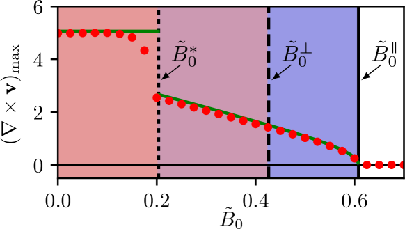
Figure 7: Maximum of the vorticity as a function of the external field strength for $\lambda=0.1$, $a=0.8$ and $b=0.1$. The green lines denote the stationary solutions of the amplitude equations (22) and (25), respectively. The red dots are obtained by numerically solving the full dynamical equation (17). Decreasing the external field strength from the onset of the instability at $\tilde{B}^{\mkern 4.0mu\vphantom{\perp}\vrule depth=0.0pt\mkern 3.0mu\vrule depth=0.0pt\mkern 5.0mu}_{0}$ we observe a stripe pattern that becomes unstable with respect to the formation of a square vortex lattice at $\tilde{B}_{0}^{\ast}$. Due to the suppression of perpendicular modes by parallel modes, the field strength $\tilde{B}_{0}^{\perp}$ obtained by linear stability analysis of the homogeneous stationary solution is not relevant.

6 Conclusions

This article studies the impact of a homogeneous, stationary external field on pattern formation in suspensions of microswimmers that exhibit mesoscale turbulence in the field-free case. Based on a numerical solution of the full model presented in section 2 and a linear stability analysis, we observe that, in the presence of an orienting field, the patterns become anisotropic and asymmetric. From a mathematical point of view, the growth rate of modes becomes dependent on the wavevector’s direction due to the broken rotational symmetry. In particular, modes perpendicular to the applied external field are suppressed for intermediate field strengths leading to the dominance of modes parallel to the field. The resulting structures can be described as stripes that travel along the field’s direction. For even higher field strengths, the instability is completely suppressed and we observe a homogeneous stationary polar state.

In the second part of the paper, we have presented a weakly nonlinear analysis of a reduced model for the effective microswimmer velocity. The model is significantly easier to handle analytically, yet still exhibits asymmetric pattern formation, which we have analyzed by deriving the amplitude equations (22) and (25). Upon an increase of the external field, there is a transition form a square vortex lattice to a traveling stripe pattern. The regularity of these patterns is strongly dependent on the coefficient $\lambda$, that determines the strength of the nonlinear advection term. When $\lambda$ is increased, defects are generated and the patterns become less regular. In this case, the amplitude equations, (22) and (25), lose their validity. This boils down to the problem already discussed in section 5.2: The nonlinear energy transfer between scales leads to a shift of the dominating mode contradicting the ansatz leading to the amplitude equations (see also F).

However, we can still observe one unique feature of the amplitude equation (25) for the stripe pattern, even for large values of $\lambda$: the equation is strongly anisotropic as is reflected by the difference of the diffusion coefficients, $D_{\mkern 4.0mu\vphantom{\perp}\vrule depth=0.0pt\mkern 3.0mu\vrule depth=0.0pt\mkern 5.0mu}$ and $D_{\perp}$. Indeed, the transport of modulations of the pattern in the direction parallel to the external field is approximately one order of magnitude faster than perpendicular to the field [see also equation (27)]. As a consequence, defects in the patterns, generated by the nonlinear advection term, will be elongated by a factor of $D_{\mkern 4.0mu\vphantom{\perp}\vrule depth=0.0pt\mkern 3.0mu\vrule depth=0.0pt\mkern 5.0mu}/D_{\perp}$ in the field’s direction. This is consistent with numerical observations shown in figure 1(c) for the full model.

As explained above, the amplitude equation (25) does not incorporate the full nonlinear advection term. This is apparent from the fact that it corresponds to the real-valued Ginzburg-Landau equation, which does not generate defects. The complex two-dimensional Ginzburg-Landau equation, however, exhibits a variety of chaotic states including one denoted as defect turbulence [72]. A preliminary comparison of this state with the dynamics of the amplitude modulations of the stripe patterns observed in the present system shows quite similar spatial structures. The derivation of an amplitude equation valid even for higher values of $\lambda$ presents an interesting future challenge.

As discussed, the external field induces polar order in the system, which leads to net transport in the field’s direction. This net transport can be modified by emerging patterns, as was demonstrated in a recent model for magnetic microswimmers, where band-like structures reflected in the inhomogeneous density of swimmers decrease the net polarization [68]. We also find an influence of emerging patterns on transport properties in our model that assumes a constant density of microswimmers on the coarse-grained level: The emerging stripe pattern in the polar order parameter field influences the traveling speed [see equation 26]. Moreover, preliminary numerical results show that the mean transport in the system is impacted in a quite complex manner. Further exploring this feedback will be especially relevant for applications, where transport properties are essential.

Anisotropic patterns emerging in microswimmer suspensions subjected to external fields have indeed already been observed in magnetotactic bacteria [73, 74]. However, in these experiments, band-like structures in the swimmer density were found, whereas in our case, we are dealing with a purely orientational effect. The stripes, visible in the vorticity, correspond to wave-like patterns in the polar order parameter field.

Appendix A Relation to the microscopic model

A detailed derivation of the continuum equations in the absence of an external field, equations (1) - (4), is given in Ref. [19]. Extending the derivation towards an external field is quite straightforward. Here, we will give a short summary of the key points.

The overdamped motion of a swimmer $\sigma$ in an ensemble of $\sigma=1,\dots,S$ identical swimmers is given by the Langevin equations for the position $\mathbf{X}^{\sigma}$ and the orientation $\mathbf{N}^{\sigma}$, respectively,

$$\dot{\mathbf{X}}^{\sigma} =v_{0}\mathbf{N}^{\sigma}+\mathbf{u}(\mathbf{X}^{\sigma})+\sqrt{2D}\boldsymbol{\xi}^{\sigma},$$ (28)

$$\dot{\mathbf{N}}^{\sigma} =\boldsymbol{\Omega}(\mathbf{X}^{\sigma})\cdot\mathbf{N}^{\sigma}+\boldsymbol{\Pi}\cdot\Big{[}a_{0}\boldsymbol{\Sigma}(\mathbf{X}^{\sigma})\cdot\mathbf{N}^{\sigma}-\nabla_{\mathbf{N}^{\sigma}}\Phi+\sqrt{1/\tau}\boldsymbol{\eta}^{\sigma}\Big{]},$$ (29)

where the functions $\boldsymbol{\xi}^{\sigma}$ and $\boldsymbol{\eta}^{\sigma}$ denote Gaussian white noise generating diffusion in the translational and rotational motion. Note, that the overdamped Langevin equations are already divided by the translational and rotational friction coefficients, respectively. Self-propulsion is introduced via the first term on the right-hand side of equation (28), involving the self-swimming speed $v_{0}$. Additionally, the swimmer is transported by advection with the averaged surrounding flow field $\mathbf{u}(\mathbf{x},t)$. The orientational motion given by equation (29) is determined, first, by rotation and alignment with the flow field. This is reflected by the terms involving the vorticity $\mathbf{\Omega}=\frac{1}{2}\big{[}(\nabla\mathbf{u})^{\mathrm{T}}-(\nabla\mathbf{u})\big{]}$ and deformation rate $\mathbf{\Sigma}=\frac{1}{2}\big{[}(\nabla\mathbf{u})^{\mathrm{T}}+(\nabla\mathbf{u})\big{]}$, respectively. In analogy to Jeffrey’s theory for oscillatory tumbling motion of elongated particles in flow [75, 76, 77], the shape parameter $a_{0}$ is given as a function of the aspect ratio, defined by length $\ell$ and diameter $d$ of the swimmers,

$$a_{0}=\frac{(\ell/d)^{2}-1}{(\ell/d)^{2}+1}.$$ (30)

Further, the projector $\boldsymbol{\Pi}=\mathbf{I}-\mathbf{N}^{\sigma}\mathbf{N}^{\sigma}$ (where $\mathbf{I}$ is the unit matrix) is introduced to conserve the length of the unit vector $\mathbf{N}^{\sigma}$. The second deterministic contribution to the orientational motion is the conservative potential $\Phi$ involving all swimmers. In the present study we consider both, pair interactions and an external contribution, that is,

$$\Phi=\sum_{\mu,\nu}\Phi_{\mathrm{int}}(\mathbf{N}^{\mu},\mathbf{N}^{\nu},r_{\mu,\nu})+\sum_{\mu}\Phi_{\mathrm{ext}}(\mathbf{N}^{\mu}).$$ (31)

The pair potential $\Phi_{\mathrm{int}}(\mathbf{N}^{\mu},\mathbf{N}^{\nu},r_{\mu,\nu})$ describes an activity-driven polar alignment of two swimmers with distance $r_{\mu,\nu}=|\mathbf{X}_{\mu}-\mathbf{X}_{\nu}|\geq r$,

$$\Phi_{\mathrm{int}}(\mathbf{N}^{\mu},\mathbf{N}^{\nu},r_{\mu,\nu})=-\frac{\gamma_{0}v_{0}}{2}\mathbf{N}^{\mu}\cdot\mathbf{N}^{\nu}\Theta(r-r_{\mu,\nu}),$$ (32)

where $\gamma_{0}$ is the strength of the interaction, and $\Theta(x)=1$ for $x\geq 0$ and zero otherwise. Note that this is a simplified ansatz that describes the polar alignment of neighboring swimmers due to near-field hydrodynamics interactions [65], an effect that has been observed experimentally [3]. Finally, the external potential for swimmer $\mu$ is given by

$$\Phi_{\mathrm{ext}}(\mathbf{N}^{\mu})=-B_{0}\frac{v_{0}}{\ell}\mathbf{h}\cdot\mathbf{N}^{\mu},$$ (33)

where the unit vector $\mathbf{h}$ denotes the field’s direction. Here, we already introduced the potential in such a way that the field’s magnitude relative to the active time scale $\ell/v_{0}$ defines the dimensionless external field strength $B_{0}$. The dimension of the full prefactor $B_{0}v_{0}/\ell$ appearing in equation (33) then is an inverse time due to the scaling of the Langevin equations (28) and (29).

Coming back to equations (28) and (29), far-field hydrodynamic interactions are taken into account by the coupling terms involving the average surrounding flow field $\mathbf{u}$. At low Reynolds numbers, this field is determined by the Stokes equation, augmented by an active contribution to the stress tensor, which, in turn depends on the order parameter. This coupling eventually leads to equation (4). Due to the lengthy derivation of the active stress we refer to our previous publication [19] for details.

The next step is to obtain the Fokker-Planck equation for the one-particle probability density function $\mathcal{P}(\mathbf{x},\mathbf{n},t)$, which gives the probability to find a swimmer at position $\mathbf{x}$ with orientation $\mathbf{n}$ at time $t$. To this end, we assume a constant swimmer density $\rho(\mathbf{x},t)=\rho$ and employ a mean-field approximation to treat the two-particle correlations stemming from conservative interactions. We then project onto orientational moments $\overline{\mathbf{n}}$, $\overline{\mathbf{n}\mathbf{n}}$, … of $\mathcal{P}(\mathbf{x},\mathbf{n},t)$, which are directly connected to the polar order parameter $\mathbf{P}$ and the nematic order parameter $\mathbf{Q}$ via

$$\mathbf{P}=\overline{\mathbf{n}},\qquad\mathbf{Q}=\overline{\mathbf{n}\mathbf{n}}-\mathbf{I}/3.$$ (34)

Following our previous studies [18, 19] we apply a closure relation for the nematic order parameter,

$$\mathbf{Q}=q(\mathbf{P}\mathbf{P}-(\mathbf{P}\cdot\mathbf{P})\mathbf{I}/3)+\lambda_{\mathrm{K}}\boldsymbol{\Sigma},$$ (35)

where the coefficients $q$ and $\lambda_{\mathrm{K}}$ can be calculated analytically [19]. This is an extension of the Doi closure for passive particles, which incorporates the fact that active particles always generate flow gradients affecting the local nematic order. For moments higher than the second we apply the so-called Hand-closure [78]. The details of the procedure are discussed in [19].

Finally, we arrive at a closed dynamic equation for the polar order parameter $\mathbf{P}$, given by equation (6) that includes a coupling to the Stokes equation (4). The two coefficients $c_{\mathrm{I}}$ and $c_{\mathrm{F}}$, not already specified in the main text, are given by

$$c_{\mathrm{I}}=\frac{8}{9}\tau\rho\gamma_{0}v_{0}r^{3},\qquad c_{\mathrm{F}}=\frac{f_{0}\rho\ell^{2}}{10\mu v_{0}},$$ (36)

where $f_{0}$ denotes the strength of the force dipole exerted by every swimmer on the surrounding fluid, and $\mu$ is the effective viscosity of the suspension [19].

Appendix B Numerical methods

Our numerical results are obtained by solving the dynamical equations (6) or (17) using the Runge–Kutta–Fehlberg method (RKF45) [79]. We use a finite-difference discretization of the spatial derivatives on a periodic grid consisting of $256\times 256$ points. For the purpose of visualization, we have increased the resolution in figure 1 by cubic interpolation. The incompressibility condition is enforced by a pressure-correction method [80]. In the case of the full model, the Stokes equation (4) is solved applying a stream-function approach [80]. If not otherwise stated, we apply the homogeneous stationary solution introduced in section 4.1 as initial conditions and add small random variations.

Appendix C Details of the linear stability analysis

In the following, we present the calculation of the complex growth rate $\sigma$ [see equations (4.2) and (16)] determining the stability of the homogeneous stationary solution. To this end, we will first eliminate the dependence of the linearized system on the perturbations $\delta\hat{\mathbf{u}}$, $\delta\hat{p}$ and $\delta\hat{q}$, thus reducing the set of variables to just the perturbation of the polar order parameter, $\delta\hat{\mathbf{P}}$.

As a first step we insert the perturbed solution [see equation (12) and (13) in the main text] into the Stokes equation (4) and linearize, yielding

$$-|\mathbf{k}|^{2}\delta\hat{\mathbf{u}}=c_{\mathrm{F}}\bigg{(}\rmi 6c_{\mathrm{I}}k_{\mkern 4.0mu\vphantom{\perp}\vrule depth=0.0pt\mkern 3.0mu\vrule depth=0.0pt\mkern 5.0mu}P_{0}\delta\hat{\mathbf{P}}-|\mathbf{k}|^{2}\delta\hat{\mathbf{P}}+\frac{1}{28}|\mathbf{k}|^{4}\delta\hat{\mathbf{P}}\bigg{)}+i\mathbf{k}\delta\hat{p}.$$ (37)

We multiply equation (37) by the wavevector $\mathbf{k}$ and employ the incompressibility conditions which, for the perturbed system, yield $\mathbf{k}\cdot\delta\hat{\mathbf{u}}=0$ and $\mathbf{k}\cdot\delta\hat{\mathbf{P}}=0$. From this, we find that the pressure perturbation amplitude must satisfy $\delta\hat{p}=0$. Equation (37) then yields the perturbation $\delta\hat{\mathbf{u}}$ as a function of the perturbation of the polar order parameter,

$$\delta\hat{\mathbf{u}}=c_{\mathrm{F}}\Bigg{(}-\rmi\frac{6c_{\mathrm{I}}k_{\mkern 4.0mu\vphantom{\perp}\vrule depth=0.0pt\mkern 3.0mu\vrule depth=0.0pt\mkern 5.0mu}P_{0}}{|\mathbf{k}|^{2}}+1-\frac{1}{28}|\mathbf{k}|^{2}\Bigg{)}\delta\hat{\mathbf{P}}.$$ (38)

We now consider the equation of motion for the polar order parameter $\mathbf{P}$, equation (6). Performing the linearization yields

$$\eqalign{\sigma\delta\hat{P}_{\mkern 4.0mu\vphantom{\perp}\vrule depth=0.0pt\mkern 3.0mu\vrule depth=0.0pt\mkern 5.0mu}=&-\rmi\lambda_{0}k_{\mkern 4.0mu\vphantom{\perp}\vrule depth=0.0pt\mkern 3.0mu\vrule depth=0.0pt\mkern 5.0mu}P_{0}\delta\hat{P}_{\mkern 4.0mu\vphantom{\perp}\vrule depth=0.0pt\mkern 3.0mu\vrule depth=0.0pt\mkern 5.0mu}-\alpha\delta\hat{P}_{\mkern 4.0mu\vphantom{\perp}\vrule depth=0.0pt\mkern 3.0mu\vrule depth=0.0pt\mkern 5.0mu}-3\beta P_{0}^{2}\delta\hat{P}_{\mkern 4.0mu\vphantom{\perp}\vrule depth=0.0pt\mkern 3.0mu\vrule depth=0.0pt\mkern 5.0mu}-\Gamma_{2}|\mathbf{k}|^{2}\delta\hat{P}_{\mkern 4.0mu\vphantom{\perp}\vrule depth=0.0pt\mkern 3.0mu\vrule depth=0.0pt\mkern 5.0mu}-\Gamma_{4}|\mathbf{k}|^{4}\delta\hat{P}_{\mkern 4.0mu\vphantom{\perp}\vrule depth=0.0pt\mkern 3.0mu\vrule depth=0.0pt\mkern 5.0mu}\\ &-\frac{4}{5}c_{\mathrm{I}}B_{0}P_{0}\delta\hat{P}_{\mkern 4.0mu\vphantom{\perp}\vrule depth=0.0pt\mkern 3.0mu\vrule depth=0.0pt\mkern 5.0mu}-\rmi\frac{2}{15}a_{0}P_{\mathrm{r}}B_{0}k_{\mkern 4.0mu\vphantom{\perp}\vrule depth=0.0pt\mkern 3.0mu\vrule depth=0.0pt\mkern 5.0mu}\delta\hat{u}_{\mkern 4.0mu\vphantom{\perp}\vrule depth=0.0pt\mkern 3.0mu\vrule depth=0.0pt\mkern 5.0mu}-\rmi k_{\mkern 4.0mu\vphantom{\perp}\vrule depth=0.0pt\mkern 3.0mu\vrule depth=0.0pt\mkern 5.0mu}\delta\hat{q}+\rmi\kappa k_{\mkern 4.0mu\vphantom{\perp}\vrule depth=0.0pt\mkern 3.0mu\vrule depth=0.0pt\mkern 5.0mu}\delta\hat{u}_{\mkern 4.0mu\vphantom{\perp}\vrule depth=0.0pt\mkern 3.0mu\vrule depth=0.0pt\mkern 5.0mu}P_{0},\\ \sigma\delta\hat{P}_{\perp}=&-\rmi\lambda_{0}k_{\mkern 4.0mu\vphantom{\perp}\vrule depth=0.0pt\mkern 3.0mu\vrule depth=0.0pt\mkern 5.0mu}P_{0}\delta\hat{P}_{\perp}-\alpha\delta\hat{P}_{\perp}-\beta P_{0}^{2}\delta\hat{P}_{\perp}-\Gamma_{2}|\mathbf{k}|^{2}\delta\hat{P}_{\perp}-\Gamma_{4}|\mathbf{k}|^{4}\delta\hat{P}_{\perp}\\ &-\frac{3}{5}c_{\mathrm{I}}B_{0}P_{0}\delta\hat{P}_{\perp}-\rmi\frac{1}{15}a_{0}P_{\mathrm{r}}B_{0}(k_{\mkern 4.0mu\vphantom{\perp}\vrule depth=0.0pt\mkern 3.0mu\vrule depth=0.0pt\mkern 5.0mu}\delta\hat{u}_{\perp}+k_{\perp}\delta\hat{u}_{\mkern 4.0mu\vphantom{\perp}\vrule depth=0.0pt\mkern 3.0mu\vrule depth=0.0pt\mkern 5.0mu})-\rmi k_{\perp}\delta\hat{q}\\ &+\rmi\frac{1}{2}\big{(}k_{\mkern 4.0mu\vphantom{\perp}\vrule depth=0.0pt\mkern 3.0mu\vrule depth=0.0pt\mkern 5.0mu}\delta\hat{u}_{\perp}-k_{\perp}\delta\hat{u}_{\mkern 4.0mu\vphantom{\perp}\vrule depth=0.0pt\mkern 3.0mu\vrule depth=0.0pt\mkern 5.0mu}\big{)}P_{0}+\rmi\frac{1}{2}\kappa\big{(}k_{\mkern 4.0mu\vphantom{\perp}\vrule depth=0.0pt\mkern 3.0mu\vrule depth=0.0pt\mkern 5.0mu}\delta\hat{u}_{\perp}+k_{\perp}\delta\hat{u}_{\mkern 4.0mu\vphantom{\perp}\vrule depth=0.0pt\mkern 3.0mu\vrule depth=0.0pt\mkern 5.0mu}\big{)}P_{0}.}$$ (39)

We can eliminate the dependence of equation (39) on the velocity perturbation $\delta\hat{\mathbf{u}}$ by inserting equation (38). The reduced system can then be written as

$$\sigma\delta\hat{\mathbf{P}}=-i\mathbf{k}\delta\hat{q}+\mathbf{M}(\mathbf{k})\cdot\delta\hat{\mathbf{P}},$$ (40)

where the components of the Jacobian matrix $\mathbf{M}(\mathbf{k})$ are given by

$$M_{{\mkern 4.0mu\vphantom{\perp}\vrule depth=0.0pt\mkern 3.0mu\vrule depth=0.0pt\mkern 5.0mu}{\mkern 4.0mu\vphantom{\perp}\vrule depth=0.0pt\mkern 3.0mu\vrule depth=0.0pt\mkern 5.0mu}}(\mathbf{k})= -\alpha-3\beta P_{0}^{2}-\Gamma_{2}|\mathbf{k}|^{2}-\Gamma_{4}|\mathbf{k}|^{4}-\rmi\lambda_{0}k_{\mkern 4.0mu\vphantom{\perp}\vrule depth=0.0pt\mkern 3.0mu\vrule depth=0.0pt\mkern 5.0mu}P_{0}-\frac{4}{5}B_{0}c_{\mathrm{I}}P_{0}$$

$$-\frac{4}{5}P_{\mathrm{r}}c_{\mathrm{F}}c_{\mathrm{I}}a_{0}B_{0}\frac{k_{\mkern 4.0mu\vphantom{\perp}\vrule depth=0.0pt\mkern 3.0mu\vrule depth=0.0pt\mkern 5.0mu}^{2}}{|\mathbf{k}|^{2}}P_{0}-\rmi\frac{2}{15}a_{0}B_{0}c_{\mathrm{F}}P_{\mathrm{r}}k_{\mkern 4.0mu\vphantom{\perp}\vrule depth=0.0pt\mkern 3.0mu\vrule depth=0.0pt\mkern 5.0mu}\Big{(}1-|\mathbf{k}|^{2}/28\Big{)}$$

$$+6\kappa c_{\mathrm{I}}c_{\mathrm{F}}\frac{k_{\mkern 4.0mu\vphantom{\perp}\vrule depth=0.0pt\mkern 3.0mu\vrule depth=0.0pt\mkern 5.0mu}^{2}}{|\mathbf{k}|^{2}}P_{0}^{2}+\rmi\kappa c_{\mathrm{F}}k_{\mkern 4.0mu\vphantom{\perp}\vrule depth=0.0pt\mkern 3.0mu\vrule depth=0.0pt\mkern 5.0mu}\Big{(}1-|\mathbf{k}|^{2}/28\Big{)}P_{0},$$

$$M_{{\mkern 4.0mu\vphantom{\perp}\vrule depth=0.0pt\mkern 3.0mu\vrule depth=0.0pt\mkern 5.0mu}\perp}(\mathbf{k})= \ 0,$$ (42)

$$M_{\perp{\mkern 4.0mu\vphantom{\perp}\vrule depth=0.0pt\mkern 3.0mu\vrule depth=0.0pt\mkern 5.0mu}}(\mathbf{k})= \ 0,$$ (43)

$$M_{\perp\perp}(\mathbf{k})= -\alpha-\beta P_{0}^{2}-\Gamma_{2}|\mathbf{k}|^{2}-\Gamma_{4}|\mathbf{k}|^{4}-\rmi\lambda_{0}k_{\mkern 4.0mu\vphantom{\perp}\vrule depth=0.0pt\mkern 3.0mu\vrule depth=0.0pt\mkern 5.0mu}P_{0}-\frac{3}{5}B_{0}c_{\mathrm{I}}P_{0}$$

$$-\frac{2}{5}P_{\mathrm{r}}c_{\mathrm{F}}c_{\mathrm{I}}a_{0}B_{0}\frac{k_{\mkern 4.0mu\vphantom{\perp}\vrule depth=0.0pt\mkern 3.0mu\vrule depth=0.0pt\mkern 5.0mu}^{2}-k_{\perp}^{2}}{|\mathbf{k}|^{2}}P_{0}$$

$$-\rmi\frac{1}{15}a_{0}B_{0}c_{\mathrm{F}}P_{\mathrm{r}}\frac{k_{\mkern 4.0mu\vphantom{\perp}\vrule depth=0.0pt\mkern 3.0mu\vrule depth=0.0pt\mkern 5.0mu}^{2}-k_{\perp}^{2}}{k_{\mkern 4.0mu\vphantom{\perp}\vrule depth=0.0pt\mkern 3.0mu\vrule depth=0.0pt\mkern 5.0mu}}\Big{(}1-|\mathbf{k}|^{2}/28\Big{)}$$

$$+\frac{3\kappa c_{\mathrm{I}}c_{\mathrm{F}}}{|\mathbf{k}|^{2}}\Big{[}k_{\mkern 4.0mu\vphantom{\perp}\vrule depth=0.0pt\mkern 3.0mu\vrule depth=0.0pt\mkern 5.0mu}^{2}(1+\kappa)+k_{\perp}^{2}(1-\kappa)\Big{]}P_{0}^{2}$$

$$+\frac{\rmi\kappa c_{\mathrm{F}}}{2k_{\mkern 4.0mu\vphantom{\perp}\vrule depth=0.0pt\mkern 3.0mu\vrule depth=0.0pt\mkern 5.0mu}}\Big{[}k_{\mkern 4.0mu\vphantom{\perp}\vrule depth=0.0pt\mkern 3.0mu\vrule depth=0.0pt\mkern 5.0mu}^{2}(1+\kappa)+k_{\perp}^{2}(1-\kappa)\Big{]}\Big{(}1-|\mathbf{k}|^{2}/28\Big{)}P_{0}.$$

Equation (40) still involves the perturbation $\delta\hat{q}$ of the Lagrange multiplier. Utilizing again the incompressibility condition for the polar order parameter field $\mathbf{P}$, yielding $\mathbf{k}\cdot\delta\hat{\mathbf{P}}=0$, and equation (40), we find that the perturbation $\delta\hat{q}$ must satisfy

$$\delta\hat{q}=-\rmi\frac{\mathbf{k}}{|\mathbf{k}|^{2}}\cdot\mathbf{M}\cdot\delta\hat{\mathbf{P}}.$$ (45)

Inserting equation (45) into equation (40) we can identify the projector $\mathbf{\Pi}(\mathbf{k})=\mathbf{I}-\mathbf{k}\mathbf{k}/|\mathbf{k}|^{2}$. With this, we obtain equation (14) in the main text, giving a linearized system involving only perturbations of $\mathbf{P}$. The complex growth rate can now be readily calculated as solution of the eigenvalue problem [equation (14)] via

$$\sigma(\mathbf{k})=\frac{k_{\perp}^{2}}{|\mathbf{k}|^{2}}M_{{\mkern 4.0mu\vphantom{\perp}\vrule depth=0.0pt\mkern 3.0mu\vrule depth=0.0pt\mkern 5.0mu}{\mkern 4.0mu\vphantom{\perp}\vrule depth=0.0pt\mkern 3.0mu\vrule depth=0.0pt\mkern 5.0mu}}+\frac{k_{\mkern 4.0mu\vphantom{\perp}\vrule depth=0.0pt\mkern 3.0mu\vrule depth=0.0pt\mkern 5.0mu}^{2}}{|\mathbf{k}|^{2}}M_{\perp\perp}-\frac{k_{\mkern 4.0mu\vphantom{\perp}\vrule depth=0.0pt\mkern 3.0mu\vrule depth=0.0pt\mkern 5.0mu}k_{\perp}}{|\mathbf{k}|^{2}}\Big{(}M_{{\mkern 4.0mu\vphantom{\perp}\vrule depth=0.0pt\mkern 3.0mu\vrule depth=0.0pt\mkern 5.0mu}\perp}+M_{\perp{\mkern 4.0mu\vphantom{\perp}\vrule depth=0.0pt\mkern 3.0mu\vrule depth=0.0pt\mkern 5.0mu}}\Big{)}.$$ (46)

For the explicit form of $\sigma(\mathbf{k})$, see equations (4.2) and (16) in the main text.

Appendix D Coefficients in the reduced and rescaled model

Four dimensionless coefficients remain in the reduced and rescaled model equation (17). These are related to the coefficients of the full model given by equations (1), (2), (3) and (7) via

$$\lambda =\sqrt{\frac{5}{3c_{\mathrm{I}}}}\sqrt{\frac{-2\Gamma_{4}}{\Gamma_{2}}}\frac{1}{\Gamma_{2}}\lambda_{0},$$ (47)

$$a =1-\frac{4\Gamma_{4}}{\Gamma_{2}^{2}}\alpha,$$ (48)

$$b =\frac{4\Gamma_{4}}{\Gamma_{2}^{2}}\frac{5}{3c_{\mathrm{I}}}\beta,$$ (49)

$$\tilde{B}_{0} =\frac{2}{3}\frac{4\Gamma_{4}}{\Gamma_{2}^{2}}\sqrt{\frac{3c_{\mathrm{I}}}{5}}B_{0}.$$ (50)

Appendix E Details of the weakly nonlinear analysis

Here we present technical details for the weakly nonlinear analysis for the case $\tilde{B}_{0}>0$. The analysis for the case $\tilde{B}_{0}=0$ is analogous, but less complex due to the overall rotational symmetry. In fact, the only non-standard feature in the field-free case is the coupling between the two leading-order amplitudes, see equation (22).

As introduced in section 5.1.2, the parameter $\varepsilon$ denotes the distance to the bifurcation occurring at $\tilde{B}_{0}=\tilde{B}^{\mkern 4.0mu\vphantom{\perp}\vrule depth=0.0pt\mkern 3.0mu\vrule depth=0.0pt\mkern 5.0mu}_{0}$ (when starting from large fields, where the system is homogeneous). At $\tilde{B}_{0}=\tilde{B}^{\mkern 4.0mu\vphantom{\perp}\vrule depth=0.0pt\mkern 3.0mu\vrule depth=0.0pt\mkern 5.0mu}_{0}$, the instability sets in, that is, perturbations with a parallel wavevector start to grow and we observe a transition to a stripe pattern. Using the definitions of the long time and space scales, $T=\varepsilon^{2}t$ and $\mathbf{X}=\varepsilon(\mathbf{x}-\mathbf{v}_{\mathrm{g}}t)$, the derivatives in the dynamic equation (17) for the effective velocity $\mathbf{v}$ are replaced by

$$\eqalign{\partial_{t}&\rightarrow\quad\partial_{t}-\varepsilon v^{\mkern 4.0mu\vphantom{\perp}\vrule depth=0.0pt\mkern 3.0mu\vrule depth=0.0pt\mkern 5.0mu}_{\mathrm{g}}\partial_{X_{\mkern 4.0mu\vphantom{\perp}\vrule depth=0.0pt\mkern 3.0mu\vrule depth=0.0pt\mkern 5.0mu}}-\varepsilon v^{\perp}_{\mathrm{g}}\partial_{X_{\perp}}+\varepsilon^{2}\partial_{T},\\ \partial_{x_{\mkern 4.0mu\vphantom{\perp}\vrule depth=0.0pt\mkern 3.0mu\vrule depth=0.0pt\mkern 5.0mu}}&\rightarrow\quad\partial_{x_{\mkern 4.0mu\vphantom{\perp}\vrule depth=0.0pt\mkern 3.0mu\vrule depth=0.0pt\mkern 5.0mu}}+\varepsilon\partial_{X_{\mkern 4.0mu\vphantom{\perp}\vrule depth=0.0pt\mkern 3.0mu\vrule depth=0.0pt\mkern 5.0mu}},\qquad\quad\partial_{x_{\perp}}\rightarrow\quad\partial_{x_{\perp}}+\varepsilon\partial_{X_{\perp}},\\ \nabla^{2}&\rightarrow\quad\partial^{2}_{x_{\mkern 4.0mu\vphantom{\perp}\vrule depth=0.0pt\mkern 3.0mu\vrule depth=0.0pt\mkern 5.0mu}}+\partial^{2}_{x_{\perp}}+\varepsilon\Big{(}2\partial_{x_{\mkern 4.0mu\vphantom{\perp}\vrule depth=0.0pt\mkern 3.0mu\vrule depth=0.0pt\mkern 5.0mu}}\partial_{X_{\mkern 4.0mu\vphantom{\perp}\vrule depth=0.0pt\mkern 3.0mu\vrule depth=0.0pt\mkern 5.0mu}}+2\partial_{x_{\perp}}\partial_{X_{\perp}}\Big{)}+\varepsilon^{2}\Big{(}\partial^{2}_{X_{\mkern 4.0mu\vphantom{\perp}\vrule depth=0.0pt\mkern 3.0mu\vrule depth=0.0pt\mkern 5.0mu}}+\partial^{2}_{X_{\perp}}\Big{)},\\ \nabla^{4}&\rightarrow\quad\partial^{4}_{x_{\mkern 4.0mu\vphantom{\perp}\vrule depth=0.0pt\mkern 3.0mu\vrule depth=0.0pt\mkern 5.0mu}}+\partial^{4}_{x_{\perp}}+2\partial^{2}_{x_{\mkern 4.0mu\vphantom{\perp}\vrule depth=0.0pt\mkern 3.0mu\vrule depth=0.0pt\mkern 5.0mu}}\partial^{2}_{x_{\perp}}\\ &\qquad+\varepsilon\Big{(}4\partial^{3}_{x_{\mkern 4.0mu\vphantom{\perp}\vrule depth=0.0pt\mkern 3.0mu\vrule depth=0.0pt\mkern 5.0mu}}\partial_{X_{\mkern 4.0mu\vphantom{\perp}\vrule depth=0.0pt\mkern 3.0mu\vrule depth=0.0pt\mkern 5.0mu}}+4\partial^{3}_{x_{\perp}}\partial_{X_{\perp}}+4\partial^{2}_{x_{\mkern 4.0mu\vphantom{\perp}\vrule depth=0.0pt\mkern 3.0mu\vrule depth=0.0pt\mkern 5.0mu}}\partial_{x_{\perp}}\partial_{X_{\perp}}+4\partial^{2}_{x_{\perp}}\partial_{x_{\mkern 4.0mu\vphantom{\perp}\vrule depth=0.0pt\mkern 3.0mu\vrule depth=0.0pt\mkern 5.0mu}}\partial_{X_{\mkern 4.0mu\vphantom{\perp}\vrule depth=0.0pt\mkern 3.0mu\vrule depth=0.0pt\mkern 5.0mu}}\Big{)}\\ &\qquad+\varepsilon^{2}\Big{(}6\partial^{2}_{x_{\mkern 4.0mu\vphantom{\perp}\vrule depth=0.0pt\mkern 3.0mu\vrule depth=0.0pt\mkern 5.0mu}}\partial^{2}_{X_{\mkern 4.0mu\vphantom{\perp}\vrule depth=0.0pt\mkern 3.0mu\vrule depth=0.0pt\mkern 5.0mu}}+6\partial^{2}_{x_{\perp}}\partial^{2}_{X_{\perp}}+2\partial^{2}_{x_{\mkern 4.0mu\vphantom{\perp}\vrule depth=0.0pt\mkern 3.0mu\vrule depth=0.0pt\mkern 5.0mu}}\partial^{2}_{X_{\perp}}+2\partial^{2}_{x_{\perp}}\partial^{2}_{X_{\mkern 4.0mu\vphantom{\perp}\vrule depth=0.0pt\mkern 3.0mu\vrule depth=0.0pt\mkern 5.0mu}}+\dots\\ &\qquad\dots+8\partial_{x_{\mkern 4.0mu\vphantom{\perp}\vrule depth=0.0pt\mkern 3.0mu\vrule depth=0.0pt\mkern 5.0mu}}\partial_{x_{\perp}}\partial_{X_{\mkern 4.0mu\vphantom{\perp}\vrule depth=0.0pt\mkern 3.0mu\vrule depth=0.0pt\mkern 5.0mu}}\partial_{X_{\perp}}\Big{)}+\mathcal{O}(\varepsilon^{3}).}$$

Note that for the case $\tilde{B}_{0}=0$ the group velocity vanishes, $v^{\mkern 4.0mu\vphantom{\perp}\vrule depth=0.0pt\mkern 3.0mu\vrule depth=0.0pt\mkern 5.0mu}_{\mathrm{g}}=v^{\perp}_{\mathrm{g}}=0$. This is due to the rotational symmetry and, thus, the absence of net transport in the system. In the present case, however, the rotational symmetry is broken and, near the onset of the instability at $\tilde{B}_{0}^{\mkern 4.0mu\vphantom{\perp}\vrule depth=0.0pt\mkern 3.0mu\vrule depth=0.0pt\mkern 5.0mu}$, only perturbations with a parallel wavevector grow. Therefore, we expand the effective velocity field $\mathbf{v}=(v_{\mkern 4.0mu\vphantom{\perp}\vrule depth=0.0pt\mkern 3.0mu\vrule depth=0.0pt\mkern 5.0mu},v_{\perp})$ in orders of $\varepsilon$ incorporating only parallel modes characterized by multiples of the critical wavenumber. The full expansion is given in equation (24) in the main text. Similarly, we expand the Lagrange multiplier $q$ that enforces the incompressibility constraint using only parallel modes,

$$q(\mathbf{x},t,\mathbf{X},T)=q_{0}+\sum_{n=1}^{\infty}\sum_{m=0}^{n}\varepsilon^{n}q_{n,m}(\mathbf{X},T)\rme^{\rmi m(x_{\mkern 4.0mu\vphantom{\perp}\vrule depth=0.0pt\mkern 3.0mu\vrule depth=0.0pt\mkern 5.0mu}-c_{\mkern 4.0mu\vphantom{\perp}\vrule depth=0.0pt\mkern 3.0mu\vrule depth=0.0pt\mkern 5.0mu}t)}+\mathrm{c.c.}\,.$$ (51)

Finally, the traveling speed $c^{\mkern 4.0mu\vphantom{\perp}\vrule depth=0.0pt\mkern 3.0mu\vrule depth=0.0pt\mkern 5.0mu}$ is also expanded in orders of $\varepsilon$,

$$c^{\mkern 4.0mu\vphantom{\perp}\vrule depth=0.0pt\mkern 3.0mu\vrule depth=0.0pt\mkern 5.0mu}=c_{0}^{\mkern 4.0mu\vphantom{\perp}\vrule depth=0.0pt\mkern 3.0mu\vrule depth=0.0pt\mkern 5.0mu}+\sum_{n=1}^{\infty}\varepsilon^{n}c_{n}^{\mkern 4.0mu\vphantom{\perp}\vrule depth=0.0pt\mkern 3.0mu\vrule depth=0.0pt\mkern 5.0mu},$$ (52)

where the zeroth component is proportional to the homogeneous stationary solution $V_{0}$, i.e., $c_{0}^{\mkern 4.0mu\vphantom{\perp}\vrule depth=0.0pt\mkern 3.0mu\vrule depth=0.0pt\mkern 5.0mu}=\lambda V_{0}$ [see equation (20)]. Now, we insert all expansions [equations (24), (52) and (51)] into equation (17) and replace all derivatives via equation (E). Sorting the resulting terms according to powers of $\varepsilon$ ($n$) and modes ($m$) we obtain solvability conditions. In the following, we successively go through the resulting equations:

• In zeroth order, $\mathcal{O}(\varepsilon^{0})$, we recover equation (18) which determines the homogeneous stationary solution $V_{0}$.

• In first order, $\mathcal{O}(\varepsilon^{1})$, we find that the contributions $v_{1,0}^{\mkern 4.0mu\vphantom{\perp}\vrule depth=0.0pt\mkern 3.0mu\vrule depth=0.0pt\mkern 5.0mu}$, $v_{1,1}^{\mkern 4.0mu\vphantom{\perp}\vrule depth=0.0pt\mkern 3.0mu\vrule depth=0.0pt\mkern 5.0mu}$, $v_{1,0}^{\perp}$, $q_{1,0}$, $q_{1,1}$ and $c_{1}^{\mkern 4.0mu\vphantom{\perp}\vrule depth=0.0pt\mkern 3.0mu\vrule depth=0.0pt\mkern 5.0mu}$ must vanish to satisfy simultaneously the dynamical equation (17) and the incompressibility condition $\nabla\cdot\mathbf{v}=0$. For $v_{1,1}^{\perp}$ we obtain

  $$0=(a-bV_{0}^{2}-\frac{3}{2}\tilde{B}_{0}V_{0})v_{1,1}^{\perp}=\varepsilon^{2}v_{1,1}^{\perp},$$ (53)

  where we used the definition of $\varepsilon$ according to equation (23). Thus, we find that $v_{1,1}^{\perp}$ actually contributes in $\mathcal{O}(\varepsilon^{3})$ to the amplitude equation obtained below.

• In second order, $\mathcal{O}(\varepsilon^{2})$, using the incompressibility constraint, we find the relation

  $$v_{2,1}^{\mkern 4.0mu\vphantom{\perp}\vrule depth=0.0pt\mkern 3.0mu\vrule depth=0.0pt\mkern 5.0mu}=\rmi\partial_{X_{\perp}}v_{1,1}^{\perp}.$$ (54)

  As a solvability condition for equation (17) we obtain for the zeroth mode ($m=0$)

  $$v_{2,0}^{\mkern 4.0mu\vphantom{\perp}\vrule depth=0.0pt\mkern 3.0mu\vrule depth=0.0pt\mkern 5.0mu}=D_{0}|v_{1,1}^{\perp}|^{2},$$ (55)

  where

  $$D_{0}=\frac{-2bV_{0}+\tilde{B}_{0}}{1+2bV_{0}^{2}+\frac{1}{2}\tilde{B}_{0}V_{0}}.$$ (56)

  Matching all terms containing the first mode ($m=1$) yields

  $$q_{2,1}=\rmi D_{\perp}v_{2,1}^{\mkern 4.0mu\vphantom{\perp}\vrule depth=0.0pt\mkern 3.0mu\vrule depth=0.0pt\mkern 5.0mu}=-D_{\perp}\partial_{X_{\perp}}v_{1,1}^{\perp},$$ (57)

  where we inserted equation (54). The coefficient $D_{\perp}$ is given in equation (27) in the main text. Equations (54) - (57) show that the second order amplitudes $v_{2,0}^{\mkern 4.0mu\vphantom{\perp}\vrule depth=0.0pt\mkern 3.0mu\vrule depth=0.0pt\mkern 5.0mu}$, $v_{2,1}^{\mkern 4.0mu\vphantom{\perp}\vrule depth=0.0pt\mkern 3.0mu\vrule depth=0.0pt\mkern 5.0mu}$ and $q_{2,1}$ are “slaved” to the first order amplitude $v_{1,1}^{\perp}$. Further, we obtain the second order contribution to the traveling speed

  $$c_{2}^{\mkern 4.0mu\vphantom{\perp}\vrule depth=0.0pt\mkern 3.0mu\vrule depth=0.0pt\mkern 5.0mu}=\lambda D_{0}|v_{1,1}^{\perp}|^{2}.$$ (58)

  All other higher order modes ($n>1$), i.e., $v_{2,2}^{\mkern 4.0mu\vphantom{\perp}\vrule depth=0.0pt\mkern 3.0mu\vrule depth=0.0pt\mkern 5.0mu}$, $v_{2,0}^{\perp}$, $v_{2,1}^{\perp}$, $v_{2,2}^{\perp}$, $q_{2,0}$, $q_{2,2}$, $\dots$ either violate the incompressibility constraint or the solvability conditions obtained from equation (17), or they contribute in orders higher than $\mathcal{O}(\varepsilon^{3})$.

• In third order, $\mathcal{O}(\varepsilon^{3})$, we finally obtain a dynamic equation for the amplitude $v_{1,1}^{\perp}$ by matching terms containing the first mode ($m=1$),

  $$\eqalign{\partial_{T}v_{1,1}^{\perp}=&+v_{1,1}^{\perp}-3b|v_{1,1}^{\perp}|^{2}v_{1,1}^{\perp}-2bV_{0}v_{2,0}^{\mkern 4.0mu\vphantom{\perp}\vrule depth=0.0pt\mkern 3.0mu\vrule depth=0.0pt\mkern 5.0mu}v_{1,1}^{\perp}-\frac{3}{2}B_{0}v_{2,0}^{\mkern 4.0mu\vphantom{\perp}\vrule depth=0.0pt\mkern 3.0mu\vrule depth=0.0pt\mkern 5.0mu}v_{1,1}^{\perp}\\ &+4\partial_{X_{\mkern 4.0mu\vphantom{\perp}\vrule depth=0.0pt\mkern 3.0mu\vrule depth=0.0pt\mkern 5.0mu}}^{2}v_{1,1}^{\perp}-\partial_{X_{\perp}}q_{2,1}^{\mkern 4.0mu\vphantom{\perp}\vrule depth=0.0pt\mkern 3.0mu\vrule depth=0.0pt\mkern 5.0mu}.}$$ (59)

  Inserting equations (55) and (57) into equation (59) and replacing $v_{1,1}^{\perp}\rightarrow A$ yields

  $$\partial_{T}A=A-g|A|^{2}A+D_{\mkern 4.0mu\vphantom{\perp}\vrule depth=0.0pt\mkern 3.0mu\vrule depth=0.0pt\mkern 5.0mu}\partial_{X_{\mkern 4.0mu\vphantom{\perp}\vrule depth=0.0pt\mkern 3.0mu\vrule depth=0.0pt\mkern 5.0mu}}^{2}A+D_{\perp}\partial_{X_{\perp}}^{2}A.$$ (60)

  The diffusion coefficients $D_{\mkern 4.0mu\vphantom{\perp}\vrule depth=0.0pt\mkern 3.0mu\vrule depth=0.0pt\mkern 5.0mu}$ and $D_{\perp}$ are given in equation (27) in the main text. Further, the coefficient of the cubic term follows as

  $$g=3b+2bV_{0}D_{0}+\frac{3}{2}\tilde{B}_{0}D_{0}.$$ (61)

Finally, scaling back to the fast time and length scales, $t$ and $\mathbf{x}$, yields the amplitude equation (25) in the main text.

Appendix F Shift of the dominating mode

Figure 8: Dominating mode $k_{\mathrm{dom}}$ in the reduced system [equation (17)] as function of the strength $\lambda$ of the advection term for the field-free case, $\tilde{B}_{0}=0$. The remaining parameters are $a=0.8$ and $b=0.1$. The data points are obtained by numerically solving [equation (17)] and determining the first maximum $\Lambda_{\mathrm{max}}$ of the spatial correlation function $\big{\langle}\mathbf{v}(\mathbf{x})\cdot\mathbf{v}(\mathbf{x}+\Delta\mathbf{x})\big{\rangle}$ (where $\big{\langle}\dots\big{\rangle}$ denotes the spatial and temporal average). The dominant mode then follows as $k_{\mathrm{dom}}=2\pi/\Lambda_{\mathrm{max}}$. To reduce the number of transient defects remaining from the initial conditions, we start from a regular vortex lattice with small random variations. For small $\lambda$, the characteristic length scale of the patterns is given by the critical mode $k_{\mathrm{c}}=1$. For larger $\lambda$, turbulent motion sets in and energy is transfered to larger scales, i.e., smaller wavenumbers.

As discussed in sections 5.2, the nonlinear advection term leads to energy transfer between different scales once its strength, $\lambda$, is large enough. As a consequence, the dominating mode in the system shifts. This shift is towards larger scales, i.e., smaller wavenumbers, for a two-dimensional system [53, 61]. To illustrate this point, we plot the dominating mode as function of the strength of the advection term $\lambda$ in figure 8. The data points are obtained numerically on the basis of the reduced and rescaled model equation (17).

Appendix G Stability of stripe pattern

The emerging pattern near the bifurcation at $\tilde{B}_{0}^{\mkern 4.0mu\vphantom{\perp}\vrule depth=0.0pt\mkern 3.0mu\vrule depth=0.0pt\mkern 5.0mu}$ manifests itself as stripes in the vorticity. With decreasing external field strength, the stripe pattern becomes unstable against the formation of a square vortex lattice. The corresponding critical field strength can be obtained by performing a suitable linear stability analysis. In contrast to section 4.2, we here add a perturbation to the stripe pattern characterized by the stationary solution $A=\sqrt{\sigma_{\mathrm{Re}}^{\mkern 4.0mu\vphantom{\perp}\vrule depth=0.0pt\mkern 3.0mu\vrule depth=0.0pt\mkern 5.0mu}/g}$ of the amplitude equation (25) (and not to the homogeneous stationary solution $V_{0}$). The full stripe pattern solution on the level of the collective microswimmer velocity $\mathbf{v}$ is given as

$$\eqalign{v_{\mkern 4.0mu\vphantom{\perp}\vrule depth=0.0pt\mkern 3.0mu\vrule depth=0.0pt\mkern 5.0mu}=V_{0}+D_{0}|A|^{2},\\ v_{\perp}=A\rme^{\rmi(x_{\mkern 4.0mu\vphantom{\perp}\vrule depth=0.0pt\mkern 3.0mu\vrule depth=0.0pt\mkern 5.0mu}-c_{\mkern 4.0mu\vphantom{\perp}\vrule depth=0.0pt\mkern 3.0mu\vrule depth=0.0pt\mkern 5.0mu}t)}+A^{\ast}\rme^{-\rmi(x_{\mkern 4.0mu\vphantom{\perp}\vrule depth=0.0pt\mkern 3.0mu\vrule depth=0.0pt\mkern 5.0mu}-c_{\mkern 4.0mu\vphantom{\perp}\vrule depth=0.0pt\mkern 3.0mu\vrule depth=0.0pt\mkern 5.0mu}t)},}$$ (62)

where $A^{\ast}$ denotes the complex conjugate of $A$. The form of the perturbation we consider is a perpendicular mode with critical wavenumber $k_{\mathrm{c}}=1$, i.e.,

$$\eqalign{v_{\mkern 4.0mu\vphantom{\perp}\vrule depth=0.0pt\mkern 3.0mu\vrule depth=0.0pt\mkern 5.0mu}=V_{0}+D_{0}|A|^{2}+\delta\hat{v}_{\mkern 4.0mu\vphantom{\perp}\vrule depth=0.0pt\mkern 3.0mu\vrule depth=0.0pt\mkern 5.0mu}\rme^{\tilde{\sigma}_{\perp}t+\rmi x_{\perp}},\\ v_{\perp}=A\rme^{\rmi(x_{\mkern 4.0mu\vphantom{\perp}\vrule depth=0.0pt\mkern 3.0mu\vrule depth=0.0pt\mkern 5.0mu}-c_{\mkern 4.0mu\vphantom{\perp}\vrule depth=0.0pt\mkern 3.0mu\vrule depth=0.0pt\mkern 5.0mu}t)}+A^{\ast}\rme^{-\rmi(x_{\mkern 4.0mu\vphantom{\perp}\vrule depth=0.0pt\mkern 3.0mu\vrule depth=0.0pt\mkern 5.0mu}-c_{\mkern 4.0mu\vphantom{\perp}\vrule depth=0.0pt\mkern 3.0mu\vrule depth=0.0pt\mkern 5.0mu}t)}+\delta\hat{v}_{\perp}\rme^{\tilde{\sigma}_{\perp}t+\rmi x_{\perp}}.}$$ (63)

Utilizing the incompressibility condition $\nabla\cdot\mathbf{v}=0$, we find $\delta\hat{v}_{\perp}=0$. We insert equation (63) into the dynamic equation for $\mathbf{v}$ [equation (17)] and obtain, after linearization, the growth rate of perpendicular modes with critical wavenumber $k_{\mathrm{c}}=1$,

$$\eqalign{\tilde{\sigma}_{\perp}=a&-b(3V_{0}^{2}+3D_{0}^{2}|A|^{4}+6P_{0}D_{0}|A|^{2}+2|A^{2}|)\\ &-2B_{0}(V_{0}+D_{0}|A|^{2}).}$$ (64)

The critical field strength $\tilde{B}^{\ast}_{0}$ defining the transition from the stripe pattern to the vortex lattice is then obtained by setting $\tilde{\sigma}_{\perp}=0$. Note that $\tilde{\sigma}_{\perp}$ depends on the amplitude of the parallel modes, $A$. This coupling is the reason why the field strength at the transition, $\tilde{B}^{\ast}_{0}$, is smaller than $\tilde{B}_{0}^{\perp}$.

References

- [1] Buttinoni I, Bialké J, Kümmel F, Löwen H, Bechinger C and Speck T 2013 Phys. Rev. Lett. 110 238301
- [2] Peruani F, Starruß J, Jakovljevic V, Søgaard-Andersen L, Deutsch A and Bär M 2012 Phys. Rev. Lett. 108 098102
- [3] Zhang H P, Be’er A, Florin E L and Swinney H L 2010 Proc. Natl. Acad. Sci. U.S.A. 107 13626–13630
- [4] Schaller V, Weber C, Semmrich C, Frey E and Bausch A R 2010 Nature 467 73–77
- [5] Sumino Y, Nagai K H, Shitaka Y, Tanaka D, Yoshikawa K, Chaté H and Oiwa K 2012 Nature 483 448–452
- [6] Rabani A, Ariel G and Be’er A 2013 PloS One 8 e83760
- [7] Vicsek T, Czirók A, Ben-Jacob E, Cohen I and Shochet O 1995 Phys. Rev. Lett. 75 1226
- [8] Stenhammar J, Nardini C, Nash R W, Marenduzzo D and Morozov A 2017 Phys. Rev. Lett. 119(2) 028005
- [9] Simha R A and Ramaswamy S 2002 Phys. Rev. Lett. 89 058101
- [10] Ramaswamy S, Simha R A and Toner J 2003 Europhys. Lett. 62 196
- [11] Toner J, Tu Y and Ramaswamy S 2005 Ann. Phys. 318 170–244
- [12] Cates M, Fielding S, Marenduzzo D, Orlandini E and Yeomans J 2008 Phys. Rev. Lett. 101 068102
- [13] Heidenreich S, Hess S and Klapp S H 2011 Phys. Rev. E 83 011907
- [14] Giomi L 2015 Phys. Rev. X 5 031003
- [15] Saintillan D and Shelley M J 2008 Phys. Rev. Lett. 100 178103
- [16] Saintillan D and Shelley M J 2013 C. R. Physique 14 497–517
- [17] Baskaran A and Marchetti M C 2008 Phys. Rev. E 77 011920
- [18] Heidenreich S, Dunkel J, Klapp S H L and Bär M 2016 Phys. Rev. E 94 020601
- [19] Reinken H, Klapp S H, Bär M and Heidenreich S 2018 Phys. Rev. E 97 022613
- [20] Lauga E and Powers T R 2009 Rep. Prog. Phys. 72 096601
- [21] Ramaswamy S 2010 Annu. Rev. Condens. Matter Phys. 1 323–345
- [22] Romanczuk P, Bär M, Ebeling W, Lindner B and Schimansky-Geier L 2012 Eur. Phys. J. Spec. Top. 202 1–162
- [23] Marchetti M, Joanny J, Ramaswamy S, Liverpool T, Prost J, Rao M and Simha R A 2013 Rev. Mod. Phys. 85 1143
- [24] Elgeti J, Winkler R G and Gompper G 2015 Rep. Prog. Phys. 78 056601
- [25] Menzel A M 2015 Phys. Rep. 554 1 – 45
- [26] Zöttl A and Stark H 2016 J. Phys. Condens. Matter 28 253001
- [27] Bechinger C, Di Leonardo R, Löwen H, Reichhardt C, Volpe G and Volpe G 2016 Rev. Mod. Phys. 88(4) 045006
- [28] Klapp S H 2016 Curr. Opin. Colloid Interface Sci. 21 76–85
- [29] Eisenbach M 2004 Chemotaxis (World Scientific Publishing Company)
- [30] Taktikos J, Zaburdaev V and Stark H 2011 Phys. Rev. E 84 041924
- [31] Garcia X, Rafaï S and Peyla P 2013 Phys. Rev. Lett. 110 138106
- [32] Martin M, Barzyk A, Bertin E, Peyla P and Rafaï S 2016 Phys. Rev. E 93 051101
- [33] Bazylinski D A and Frankel R B 2004 Nat. Rev. Microbiol. 2 217
- [34] Waisbord N, Lefèvre C, Bocquet L, Ybert C and Cottin-Bizonne C 2016 arXiv preprint arXiv:1603.00490
- [35] Nadkarni R, Barkley S and Fradin C 2013 PLoS One 8 e82064
- [36] Popp F, Armitage J P and Schüler D 2014 Nat. Commun. 5 5398
- [37] Fukui K and Asai H 1985 Biophys. J. 47 479–482
- [38] Ten Hagen B, Kümmel F, Wittkowski R, Takagi D, Löwen H and Bechinger C 2014 Nat. Commun. 5 4829
- [39] Trivedi R R, Maeda R, Abbott N L, Spagnolie S E and Weibel D B 2015 Soft matter 11 8404–8408
- [40] Sokolov A, Zhou S, Lavrentovich O D and Aranson I S 2015 Phys. Rev. E 91 013009
- [41] Schwarz L, Medina-Sánchez M and Schmidt O G 2017 Appl. Phys. Rev. 4 031301
- [42] Martel S, Mohammadi M, Felfoul O, Lu Z and Pouponneau P 2009 Int. J. Robotics Res. 28 571–582
- [43] Felfoul O, Mohammadi M, Taherkhani S, De Lanauze D, Xu Y Z, Loghin D, Essa S, Jancik S, Houle D, Lafleur M et al. 2016 Nat. Nanotechnol. 11 941
- [44] Kaiser A, Peshkov A, Sokolov A, ten Hagen B, Löwen H and Aranson I S 2014 Phys. Rev. Lett. 112 158101
- [45] Sokolov A, Apodaca M M, Grzybowski B A and Aranson I S 2010 Proc. Natl. Acad. Sci. U.S.A. 107 969–974
- [46] Jalali M A, Khoshnood A and Alam M R 2015 J. Fluid Mech. 779 669–683
- [47] Wensink H H, Dunkel J, Heidenreich S, Drescher K, Goldstein R E, Löwen H and Yeomans J M 2012 Proc. Natl. Acad. Sci. U.S.A. 109 14308–14313
- [48] Dombrowski C, Cisneros L, Chatkaew S, Goldstein R E and Kessler J O 2004 Phys. Rev. Lett. 93 098103
- [49] Zhang H, Be’er A, Smith R S, Florin E L and Swinney H L 2009 Europhys. Lett. 87 48011
- [50] Sokolov A and Aranson I S 2012 Phys. Rev. Lett. 109 248109
- [51] Lushi E, Wioland H and Goldstein R E 2014 Proc. Natl. Acad. Sci. U.S.A. 111 9733–9738
- [52] Nishiguchi D and Sano M 2015 Phys. Rev. E 92 052309
- [53] Davidson P 2015 Turbulence: an introduction for scientists and engineers (Oxford University Press)
- [54] Ilkanaiv B, Kearns D B, Ariel G and Be’er A 2017 Phys. Rev. Lett. 118 158002
- [55] Dunkel J, Heidenreich S, Bär M and Goldstein R E 2013 New J. Phys. 15 045016
- [56] Dunkel J, Heidenreich S, Drescher K, Wensink H H, Bär M and Goldstein R E 2013 Phys. Rev. Lett. 110 228102
- [57] Słomka J and Dunkel J 2015 Eur. Phys. J. ST 224 1349–1358
- [58] Oza A U, Heidenreich S and Dunkel J 2016 Eur. Phys. J. E 39 97
- [59] Bratanov V, Jenko F and Frey E 2015 Proc. Natl. Acad. Sci. U.S.A. 112 15048–15053
- [60] James M and Wilczek M 2018 Eur. Phys. J. E 41 21
- [61] James M, Bos W J and Wilczek M 2018 Phys. Rev. Fluids 3 061101(R)
- [62] Großmann R, Romanczuk P, Bär M and Schimansky-Geier L 2014 Phys. Rev. Lett. 113 258104
- [63] Großmann R, Romanczuk P, Bär M and Schimansky-Geier L 2015 Eur. Phys. J. Special Topics 224 1325–1347
- [64] Toner J and Tu Y 1998 Phys. Rev. E 58 4828
- [65] Hoell C, Löwen H and Menzel A M 2018 arXiv preprint arXiv:1807.08564
- [66] Blums E, Cebers A and Maiorov M M 1997 Magnetic fluids (Walter de Gruyter)
- [67] Rosensweig R E 2013 Ferrohydrodynamics (Courier Corporation)
- [68] Koessel F R and Jabbari-Farouji S 2018 arXiv preprint arXiv:1802.07364
- [69] Edwards S and Yeomans J 2009 Europhys. Lett. 85 18008
- [70] Cross M C and Hohenberg P C 1993 Rev. Mod. Phys. 65 851
- [71] Newell A C, Passot T and Lega J 1993 Ann. Rev. Fluid Mech. 25 399–453
- [72] Aranson I S and Kramer L 2002 Rev. Mod. Phys. 74 99
- [73] Guell D, Brenners H, Frankel R B and Hartman H 1988 Physics 139
- [74] Spormann A M 1987 FEMS Microbiol. Ecol. 3 37–45
- [75] Jeffery G B 1922 Proc. R. Soc. Lond. A 102 161–179
- [76] Hinch E J and Leal L G 1979 J. Fluid Mech. 92 591 – 508
- [77] Pedley T and Kessler J O 1992 Annu. Rev. Fluid Mech. 24 313–358
- [78] Kröger M, Ammar A and Chinesta F 2008 J. Non-Newtonian Fluid Mech. 149 50–55
- [79] Fehlberg E 1969 NASA Technical Report 315
- [80] Pozrikidis C 2011 Introduction to theoretical and computational fluid dynamics (Oxford University Press)