Extending Modular Semantics for Bipolar Weighted Argumentation (Technical Report)

Abstract.

Weighted bipolar argumentation frameworks offer a tool for decision support and social media analysis. Arguments are evaluated by an iterative procedure that takes initial weights and attack and support relations into account. Until recently, convergence of these iterative procedures was not very well understood in cyclic graphs. Mossakowski and Neuhaus recently introduced a unification of different approaches and proved first convergence and divergence results. We build up on this work, simplify and generalize convergence results and complement them with runtime guarantees. As it turns out, there is a tradeoff between semantics’ convergence guarantees and their ability to move strength values away from the initial weights. We demonstrate that divergence problems can be avoided without this tradeoff by continuizing semantics. Semantically, we extend the framework with a Duality property that assures a symmetric impact of attack and support relations. We also present a Java implementation of modular semantics and explain the practical usefulness of the theoretical ideas.

1. Introduction

Abstract argumentation Dung (1995) allows modeling arguments and their relationships in order to decide which arguments should be accepted and which should be rejected. We focus on weighted bipolar argumentation frameworks here that start with an initial weight of arguments and adapt this weight based on the strength of their attackers and supporters Baroni et al. (2015); Rago et al. (2016); Amgoud and Ben-Naim (2017); Mossakowski and Neuhaus (2018); Potyka (2018a). These frameworks can be applied to tasks like decision support Baroni et al. (2013); Rago et al. (2016), social media analysis Leite and Martins (2011); Alsinet et al. (2017) or information retrieval Thiel et al. (2017). Initial weights can be defined manually based on the reputation of arguments’ sources or computed automatically based on statistics like the success rate of a source (in decision support) or the number of likes or retweets of an argument (in social media analysis). Sentiment analysis tools can be used to extract attack and support relations automatically as well Alsinet et al. (2017).

Mossakowski and Neuhaus recently introduced a unification of different approaches by decomposing their semantics into an aggregation function that aggregates the strength of attackers and supporters and an influence function that adapts the initial weight based on the aggregate Mossakowski and Neuhaus (2018). Different combinations of aggregation and influence functions yield different semantics from the literature and axioms proposed in Amgoud and Ben-Naim (2016a, b, 2017) can be related to elementary properties of these functions. Mossakowski and Neuhaus (2018) also proved first results about the convergence of bipolar weighted argumentation models in cyclic graphs. Note that convergence is essential to obtain final strength values here. Mossakowski and Neuhaus (2018) gave convergence results for sum- and max-based aggregation functions and influence functions whose derivatives can be bounded.

We will show that all these results can be seen as special cases of the Contraction Principle from Real Analysis Rudin (1976) and can be generalized in a uniform way by replacing the assumption of bounded derivatives from Mossakowski and Neuhaus (2018) with Lipschitz continuity. This allows generalizing the convergence results and to add runtime guarantees. However, we also show that convergence guarantees derived from the contraction principle are bought at the expense of open-mindedness. That is, as the convergence guarantees of a semantics obtained from the contraction principle get stronger, its ability to change the initial weights gets weaker. We also give some new divergence examples based on a family of graphs from Mossakowski and Neuhaus (2018). In order to avoid the tradeoff between convergence guarantees and open-mindedness of semantics, we can continuize semantics as proposed in Potyka (2018a). We demonstrate that the observed divergence problems can be solved by continuization and, thus, give some additional empirical evidence for the robustness of continuous models. Subsequently, we integrate the recently introduced Duality property Potyka (2018a) into the framework by Mossakowski and Neuhaus by relating it to elementary properties of the aggregation and influence function. Finally, we present an implementation of Modular semantics in the Java library Attractor Potyka (2018b) and illustrate the practical usefulness of modular semantics.

2. BAGs and Modular Semantics

We consider weighted bipolar argumentation graphs (BAGs) as considered in Amgoud and Ben-Naim (2017) and Mossakowski and Neuhaus (2018).

Definition (BAG).

A BAG is a tuple $\mathcal{\textbf{A}}=(\mathcal{A},\mathcal{\operatorname{w}},\mathcal{R},\mathcal{S})$, where $\mathcal{A}$ is an $n$-dimensional vector of arguments, $\mathcal{\operatorname{w}}\in[0,1]^{n}$ is a weight vector that associates an initial weight $w_{i}$ with every argument $\mathcal{A}_{i}$ and $\mathcal{R}$ and $\mathcal{S}$ are binary relations on $\mathcal{A}$ called attack and support.

The parent vector $g_{i}\in\{-1,0,1\}^{n}$ of argument $\mathcal{A}_{i}$ is the vector with entries $g_{i,j}=-1$ ($1$) iff $(\mathcal{A}_{j},\mathcal{A}_{i})\in\mathcal{R}$ ($(\mathcal{A}_{j},\mathcal{A}_{i})\in\mathcal{S}$). We visualize BAGs by means of directed graphs, where nodes show the arguments with their initial weights, solid edges denote attacks and dashed edges denote supports. We let $\textit{indegree}(\mathcal{A}_{i})=\sum_{j=1}^{n}|g_{i,j}|$ be the number of attackers and supporters of $\mathcal{A}_{i}$.

Example

Figure 1 shows the directed graph for the BAG $\big{(}(a,b,c),(0.6,0.9,0.4),\{(a,b),(a,c)\},\{(b,c),(c,b)\}\big{)}$.

Figure 1. Graph for Example 2.

The parent vector of $b$ is $g_{2}=(-1,0,1)$ and shows that $b$ is attacked by $a$ and supported by $c$. Hence, $\textit{indegree}(b)=2$.

Given a BAG A, we want to assign a strength value to every argument. This can be accomplished by means of different acceptability semantics Amgoud and Ben-Naim (2017). These semantics are usually based on an iterative update procedure that may or may not converge. Therefore, we follow Mossakowski and Neuhaus (2018) and regard acceptability semantics as partial functions.

Definition (Acceptability Semantics).

An acceptability semantics is a partial function $\operatorname{Deg}_{S}$ that maps a BAG $\mathcal{\textbf{A}}=(\mathcal{A},\mathcal{\operatorname{w}},\mathcal{R},\mathcal{S})$ with $n$ arguments to an $n$-dimensional vector $\operatorname{Deg}_{S}(\mathcal{\textbf{A}})\in[0,1]^{n}$ or to $\bot$ (undefined). If $\operatorname{Deg}_{S}(\mathcal{\textbf{A}})\neq\bot$, we call the $i$-th component $\operatorname{Deg}_{S}(\mathcal{\textbf{A}})_{i}$ the final strength or acceptability degree of $\mathcal{A}_{i}$.

A modular acceptability semantics as introduced in Mossakowski and Neuhaus (2018) is an acceptability semantics that works by first aggregating the strength of attackers and supporters and then adapting the initial weight based on the aggregated value. This is accomplished by aggregation and influence functions, which satisfy some additional properties that guarantee that axioms from Amgoud and Ben-Naim (2017) are satisfied. Even though all axioms are interesting semantically, we will restrict to a subset here in order to keep the presentation simple and more general.

The aggregation and influence functions in Mossakowski and Neuhaus (2018) were supposed to be continuous. We make a stronger assumption here and assume that they are Lipschitz-continuous. Intuitively, this means that the growth of these functions is bounded by a constant. Lipschitz-continuity is also implied by the convergence conditions (bounded derivatives) in Mossakowski and Neuhaus (2018), so we do not restrict the generality of our convergence investigation. Formally, a function $f:X\rightarrow Y$ is called Lipschitz-continuous with Lipschitz constant $\lambda$ iff $\|f(x)-f(y)\|_{Y}\leq\lambda\|x-y\|_{X}$. The sets $X$ and $Y$ will contain real numbers, vectors or matrices here. We consider the maximum norm for matrices defined by $\|A\|=\max\{\sum_{j=1}^{m}|a_{i,j}|\mid 1\leq i\leq n\}$ for an $m\times n$-matrix $A=(a_{i,j})$. That is, $\|A\|$ is the largest absolute row sum in $A$. For the special case that $x\in\mathbb{R}^{n}$ is a vector (an $n\times 1$-matrix), $\|x\|$ is the largest absolute value in $x$. Notice that using the maximum norm does not mean any loss of generality because all norms are equivalent in $\mathbb{R}^{n}$ Rudin (1976) (the difference between two norms can be bounded by a constant factor).

The aggregation function requires information about the attackers and supporters, the influence function requires information about the initial weight. We regard this information as parameters of the function. We also have to express that the aggregation function depends only on the parents. As discussed in Mossakowski and Neuhaus (2018), this demand corresponds to the directionality axiom from Amgoud and Ben-Naim (2017). In order to phrase directionality, we define an equivalence relation for every parent vector $v\in\{-1,0,1\}^{n}$. Two (strength) vectors $s_{1},s_{2}$ are called equivalent with respect to a parent vector $v$, written as $s_{1}\equiv_{v}s_{2}$ iff $s_{1,i}=s_{2,i}$ whenever $v_{i}\neq 0$. That is, only the strength values of parents matter, all other strength values are ignored.

In the following, for a function $f$, we let $f^{k}$ denote the function that is obtained by applying $f$ $k$ times, that is, $f^{1}=f$ and $f^{k+1}=f^{k}\circ f$. Applying our update function repeatedly to the initial weights yields a sequence of strength vectors. The final strength values are defined as the limit of this sequence if it exists. Thus, convergence guarantees of update functions correspond to completeness guarantees of semantics. As usual, we say that an n-dimensional sequence $(s_{n})_{n\in\mathbb{N}}$, $s_{n}\in\mathbb{R}^{n}$, converges to $s$, denoted as $\lim_{n\rightarrow\infty}s_{n}=s$, iff the real sequence $(\|s_{n}-s\|)_{n\in\mathbb{N}}$ converges to $0$. That is, for every $\epsilon>0$, there is a $N\in\mathbb{N}$ such that $\|s_{m}-s\|<\epsilon$ for all $m>N$. Intuitively, this means that the $i$-th component of $(s_{n})$ converges to the $i$-th component of $s$.

We are now ready to define basic modular semantics.

Definition (Basic Modular Semantics).

A semantics $\operatorname{Deg}_{S}$ is called a basic modular semantics if there exists

1. an aggregation function $\alpha_{v}:[0,1]^{n}\rightarrow\mathbb{R}$ such that for all parent parameters $v\in\{-1,0,1\}^{n}$ and $s,s_{1},s_{2}\in[0,1]^{n}$

   • $\alpha_{v}(s_{1})=\alpha_{v}(s_{2})$ whenever $s_{1}\equiv_{v}s_{2}$, (Directionality)

   • $\alpha_{v}$ is Lipschitz-continuous, (Lipschitz-$\alpha$)

   • $\alpha_{v}(s)=0$ whenever $v=0$, (Stability-$\alpha$)

2. an influence function $\iota_{w}:\mathbb{R}\rightarrow[0,1]$ such that for all weight parameters $w\in\mathbb{R}$

   • $\iota_{w}$ is Lipschitz-continuous, (Lipschitz-$\iota$)

   • $\iota_{w}(0)=w$ (Stability-$\iota$)

and for all BAGs $\mathcal{\textbf{A}}=(\mathcal{A},\mathcal{\operatorname{w}},\mathcal{R},\mathcal{S})$, we have

$$\operatorname{Deg}_{S}(\mathcal{\textbf{A}})=\lim_{k\rightarrow\infty}f_{S}^{k}(\mathcal{\operatorname{w}}).$$

where the $i$-th component of $f_{S}:[0,1]^{n}\rightarrow[0,1]^{n}$ is defined by $\iota_{\mathcal{\operatorname{w}}_{i}}\circ\alpha_{g_{i}}$ for $i=1,\dots,n$. $f_{S}$ is called the update function of $\operatorname{Deg}_{S}$.

In practice, for the $i$-th argument $\mathcal{A}_{i}$, its parent vector $g_{i}$ serves as the parent parameter of $\alpha_{v}$ and its initial weight $\mathcal{\operatorname{w}}_{i}$ serves as the weight parameter for $\iota_{w}$. Stability-$\alpha$ and Stability-$\iota$ assure that the final strength of an argument without parents will just be its initial weight. This corresponds to the stability axiom from Amgoud and Ben-Naim (2017).

Intuitively, modular semantics compute strength values iteratively. They start with the initial strength vector $s^{(0)}=\mathcal{\operatorname{w}}$. Then, in the $k$-th step, the strength of argument $i$ is computed by first applying the aggregation function to $s^{(k-1)}$ and then applying the influence function to $\alpha_{g_{i}}(s^{(k-1)})$. That is, $s_{i}^{(k)}=\iota_{\mathcal{\operatorname{w}}_{i}}(\alpha_{g_{i}}(s^{(k-1)}))$ for $k>0$.

Aggregation Functions
Sum	$\alpha^{\Sigma}_{v}:[0,1]^{n}\rightarrow\mathbb{R}$	$\alpha^{\Sigma}_{v}(s)=\sum_{i=1}^{n}v_{i}\cdot s_{i}$	$\lambda_{v}^{\Sigma}=\sum_{i=1}^{n}|v_{i}|$
Product	$\alpha^{\Pi}_{v}:[0,1]^{n}\rightarrow[-1,1]$	$\alpha^{\Pi}_{v}(s)=\prod_{i:v_{i}=-1}(1-s_{i})-\prod_{i:v_{i}=1}(1-s_{i})$	$\lambda_{v}^{\Pi}=\sum_{i=1}^{n}|v_{i}|$
Top	$\alpha^{\textit{max}}_{v}:[0,1]^{n}\rightarrow[-1,1]$	$\alpha^{\textit{max}}_{v}(s)=M_{v}(s)-M_{-v}(s)$,	$\lambda_{v}^{\textit{max}}=\min\{2,\sum_{i=1}^{n}|v_{i}|\}$
		where $M_{v}(s)=\max\{0,v_{1}\cdot s_{1},\dots,v_{n}\cdot s_{n}\}$,
Influence Functions
Linear($\kappa$)	$\iota^{l}_{w}:[-\kappa,\kappa]\rightarrow[0,1]$	$\iota^{l}_{w}(s)=\mathcal{\operatorname{w}}-\frac{\mathcal{\operatorname{w}}}{\kappa}\cdot\max\{0,-s\}+\frac{1-\mathcal{\operatorname{w}}}{\kappa}\cdot\max\{0,s\}$	$\lambda^{l}_{w}=\frac{1}{\kappa}\max\{w,1-w\}$
Euler-based	$\iota^{e}_{w}:\mathbb{R}\rightarrow[\mathcal{\operatorname{w}}^{2},1]$	$\iota^{e}_{w}(s)=1-\frac{1-w^{2}}{1+w\cdot e^{s}}$	$\lambda^{e}_{w}=\frac{1}{4}$
p-Max($\kappa$)	$\iota^{p}_{w}:\mathbb{R}\rightarrow[0,1]$	$\iota_{\mathcal{\operatorname{w}}}^{p}=\mathcal{\operatorname{w}}-\mathcal{\operatorname{w}}\cdot h(-\frac{s}{\kappa})+\mathcal{\operatorname{w}}\cdot h(\frac{s}{\kappa})$	$\lambda^{p}_{w}=\frac{p}{\kappa}\max\{w,1-w\}$
for $p\in\mathbb{N}$		where $h(x)=\frac{\max\{0,x\}^{p}}{1+\max\{0,x\}^{p}}$

Table 1. Some aggregation and influence functions with corresponding Lipschitz constants.

Table 1 shows some examples of different aggregation and influence functions that can be found in the literature.

Proposition

The functions in Table 1 are aggregation and influence functions as defined in Definition 2. In particular, they are Lipschitz-continuous with the provided Lipschitz constants.

Proof.

Stability and Directionality can be easily checked from the definitions.

For Lipschitz-continuity, we will repeatedly use the fact that if the derivative of a function is bounded by $B$, then it is Lipschitz-continuous with Lipschitz constant $B$. This can be seen from the intermediate value theorem Rudin (1976). We will also use the fact that the derivative of a continuously differentiable function corresponds to a matrix of partial derivatives (the Jacobian matrix) Rudin (1976).

Sum: The sum-aggregation function is continuously differentiable and $\frac{\mathrm{d}\alpha_{v}}{\mathrm{d}s_{i}}=v_{i}$. Hence, $\|\alpha^{\prime}_{v}(s)\|=\sum_{i=1}^{n}|v_{i}|$.

Product: The product-aggregation function is continuously differentiable and $\frac{\mathrm{d}\alpha_{v}}{\mathrm{d}s_{i}}=-\prod_{j:v_{j}=-1,j\neq i}(1-s_{j})$ if $v_{i}=-1$, $\frac{\mathrm{d}\alpha_{v}}{\mathrm{d}s_{i}}=\prod_{j:v_{j}=1,j\neq i}(1-s_{j})$ if $v_{i}=1$ and $\frac{\mathrm{d}\alpha^{\prime}_{v}}{\mathrm{d}s_{i}}=0$ otherwise. All derivatives are bounded from above by $1$ and non-zero only if $v_{i}\in\{-1,1\}$. Therefore, $\|\alpha^{\prime}_{v}(s)\|\leq\sum_{i=1}^{n}|v_{i}|$.

Top: For vectors $s,s^{\prime}\in[0,1]^{n}$, we have $|M_{v}(s)-M_{v}(s^{\prime})|=|\max\{0,v_{1}\cdot s_{1},\dots,v_{n}\cdot s_{n}\}-\max\{0,v_{1}\cdot s^{\prime}_{1},\dots,v_{n}\cdot s^{\prime}_{n}\}|\leq|1-0|=1.$ Hence $|\alpha^{\textit{max}}_{v}(s_{1})-\alpha^{\textit{max}}_{v}(s_{2})|=|M_{v}(s)-M_{-v}(s)-\big{(}M_{v}(s^{\prime})-M_{-v}(s^{\prime})\big{)}|\leq|M_{v}(s)-M_{v}(s^{\prime})|-|M_{-v}(s)-M_{-v}(s^{\prime})\big{)}|\leq 2.$ If $v$ contains only $1$ ($0$) non-zero element, only one (zero) differences can be non-zero. Therefore, the slope is bounded by $\min\{2,\sum_{i=1}^{n}|v_{i}|\}$.

Linear($\kappa$): the function is not differentiable at $0$. However, the right derivative is $\frac{1-w}{\kappa}$ and the left derivative is $-\frac{w}{\kappa}$. Overall, the slope is bounded at every point by $\frac{1}{\kappa}\max\{w,1-w\}$.

Euler-based: Mossakowski and Neuhaus (2018) showed in the proof of Theorem 8 that the derivative of the Euler-based semantics is bounded strictly from above by $\frac{1}{4}$.

p-Max($\kappa$): For $p=1$, $\max\{0,x\}$ is not differentiable at $0$, but the slope is bounded by $p=1$ for all $x$. For $p>1$, $\max\{0,x\}^{p}$ is differentiable with derivative $\max\{0,p\cdot x^{p-1}\}$. Hence, the quotient rule of differentiation implies that the derivative of $h(x)$ is

$$\frac{\max\{0,p\cdot x^{p-1}\}\cdot(1+\max\{0,x\}^{p})-\max\{0,x\}^{p}\cdot\max\{0,p\cdot x^{p-1}\}}{(1+\max\{0,x\}^{p})^{2}}$$

$$\leq\frac{\max\{0,p\cdot x^{p-1}\}}{1+\max\{0,x\}^{p}}-\frac{\max\{0,x\}^{p}}{1+\max\{0,x\}^{p}}\cdot\frac{\max\{0,p\cdot x^{p-1}\}}{1+\max\{0,x\}^{p}}$$

$$\leq p-0=p.$$

Hence, the chain rule of differentiation implies that the derivative of $h(\frac{s}{\kappa})$ is $\frac{p}{\kappa}$. Linearity of the limit implies then differentiability of $\iota_{w}^{p}$. The derivative is piecewise linear with a discontinuity at $0$, but the slope can again be bounded. The derivative is $0$ for $s=0$, bounded by $|-\mathcal{\operatorname{w}}\cdot h^{\prime}(-\frac{s}{\kappa})|\leq\frac{p\cdot\mathcal{\operatorname{w}}}{\kappa}$ for $s<0$ and bounded by $|\mathcal{\operatorname{w}}\cdot h^{\prime}(\frac{s}{\kappa})|\leq\frac{p\cdot\mathcal{\operatorname{w}}}{\kappa}$ for $s>0$. Overall, the derivative is bounded by $\frac{p}{\kappa}\max\{w,1-w\}$. ∎

All aggregation functions that we consider here work by computing an aggregated attack and support value independently and subtracting these values. The sum-aggregation function has been used for the Euler-based semantics in Amgoud and Ben-Naim (2017) and for the quadratic energy model in Potyka (2018a). It aggregates strength values by adding them. The product-aggregation function is the aggregation function of the DF-QuAD algorithm Rago et al. (2016). Intuitively, the aggregate for attack and support is initially $1$ and the aggregates are decreased by multiplying with $(1-s)$ for an attacker or supporter with strength $s$. The top-aggregation function has been used for the top-based semantics in Amgoud and Ben-Naim (2016b) for support-only graphs and has been generalized to bipolar graphs in Mossakowski and Neuhaus (2018). It considers only the strongest attacker and supporter.

We consider three influence functions. The linear($\kappa$) influence function has a parameter $\kappa$ that we call its conservativeness for reasons that will become clear later. The function linear(1) can be seen as the influence function of the DF-QuAD algorithm in Rago et al. (2016). It moves the strength to $0$ or $1$ directly proportional to the aggregated strength values. This yields easily interpretable results, but requires that the aggregation function yields values between $-1$ and $1$. Hence, it cannot be combined with the sum-aggregation function. More generally, linear($\kappa$) requires that the aggregation function yields values between $-\kappa$ and $\kappa$. The Euler-based influence function has been used for the Euler-based semantics in Amgoud and Ben-Naim (2017). It has some nice properties but causes an asymmetry between attack and support as we discuss later. The p-Max influence function avoids this asymmetry. The p-Max influence function with $p=2$ is used for the quadratic energy model in Potyka (2018a). By increasing the parameter $p$, we increase (decrease) the influence of aggregates larger (smaller) than $1$. We add again a parameter $\kappa$ for the conservativeness.

Table 2 summarizes the building blocks of the DF-QuAD algorithm (DFQ), the Euler-based semantics (Euler) and the quadratic energy model (QE). We also add a conservativeness parameter to DFQ and QE.

Semantics	Aggregation	Influence
DFQ($\kappa$)	Product	Linear($\kappa$)
Euler	Sum	Euler-based
QE($\kappa$)	Sum	2-Max($\kappa$)

Table 2. Example semantics from the literature.

3. Convergence and Open-Mindedness

As shown in Mossakowski and Neuhaus (2018), modular acceptability semantics always converge for acyclic graphs. The claim remains true for basic modular semantics. In fact, the limit can be computed in linear time by a single pass trough the graph as we explain in the following proposition.

Proposition (Convergence and Complexity for Acyclic BAGs)

Let $\operatorname{Deg}_{S}$ be a basic modular semantics. For every acyclic BAG $\mathcal{\textbf{A}}=(\mathcal{A},\mathcal{\operatorname{w}},\mathcal{R},\mathcal{S})$ with $n$ arguments, the limit

$$\operatorname{Deg}_{S}(\mathcal{\textbf{A}})=\lim_{k\rightarrow\infty}f_{S}^{k}(\mathcal{\operatorname{w}}).$$

exists and can be computed by the following algorithm:

1. Compute a topological ordering of the arguments and set $s^{(0)}\leftarrow\mathcal{\operatorname{w}}$ and $k\leftarrow 1$.

2. Pick the next argument $\mathcal{A}_{i}$ in the order and set

   $$\operatorname{Deg}_{S}(\mathcal{\textbf{A}})_{i}=\iota_{\mathcal{\operatorname{w}}_{i}}(\alpha_{g_{i}}(s^{(k-1)})).$$

3. Set $k\leftarrow k+1$ and repeat step 2 until $k>n$.

Provided that $\alpha_{g}$ and $\iota_{w}$ can be computed in linear time, the algorithm runs in linear time.

Proof.

For the convergence proof, we can assume w.l.o.g. that the arguments are topologically ordered because A is acyclic. That is, for every edge $(\mathcal{A}_{i},\mathcal{A}_{j})$ in the graph (attack or support), we have $i<j$. We show by induction that the strength of $\mathcal{A}_{i}$ remains unchanged after iteration $i$. Since $\mathcal{A}_{1}$ has no predecessors, $s^{(k)}_{1}=\mathcal{\operatorname{w}}$ for all iterations $k$ by stability and directionality. Assume that the claim is true for the first $k-1$ arguments. Then, $s^{(m)}_{i}=s^{(k)}_{i}$ for $i=1,\dots,k-1$ and all $m>k$. That is, $s^{(m)}\equiv_{g_{k}}s^{(k)}$, so that directionality implies $s^{(m)}_{k}=s^{(k)}_{k}=(\iota_{\mathcal{\operatorname{w}}_{1}}\circ\alpha_{g_{i}})(s^{(k-1)}_{k})$ for all all $m>k$.

Hence, after $n$ iterations, the procedure is guaranteed to have converged. For the runtime analysis, we can no longer assume that the arguments are topologically ordered. However, a topological ordering can be computed in linear time Cormen et al. (2009). The naive computation of the strength values takes quadratic time. However, it is actually not necessary to compute the strength for all arguments in every iteration because the strength of $\mathcal{A}_{i}$ depends only on the strength of $\mathcal{A}_{1},\dots,\mathcal{A}_{i-1}$. Hence, it suffices to compute only $s_{i}$ in iteration $i$. Then the overall runtime is linear. ∎

We will now apply the contraction principle to unify and to generalize the convergence guarantees from Mossakowski and Neuhaus (2018). A contraction is a Lipschitz-continuous function with Lipschitz-constant strictly smaller than $1$. The contraction principle states intuitively that every contraction has a unique fixed-point that can be reached by applying the function repeatedly starting from an arbitrary point.

Lemma (Contraction Principle)

If $S$ is a complete metric space and if $f:S\rightarrow S$ is a contraction, then there exists one and only one $x^{*}\in S$ such that $f(x^{*})=x^{*}$. In particular, $\lim_{n\rightarrow\infty}f^{n}(x)=x^{*}$ for all $x\in S$.

A proof of the contraction principle can be found, for example, in Rudin (1976). The set $[0,1]^{n}$ of strength vectors with distance $d(x,y)=\|x-y\|$ defined by the maximum norm is indeed a complete metric space. Given a BAG with $n$ arguments such that $(\iota_{\mathcal{\operatorname{w}}_{i}}\circ\alpha_{g_{i}})$ is a contraction for all $i=1,\dots,n$, the contraction principle guarantees that the strength values converge. As we will explain soon, the convergence results in Mossakowski and Neuhaus (2018) are special cases of the following result. In particular, we can relate convergence time to the Lipschitz-constants.

Proposition (Convergence and Complexity for Contractive BAGs)

Let A be a BAG, let $\operatorname{Deg}_{S}$ be a basic modular semantics and let $\lambda_{\mathcal{\textbf{A}},S}=\max_{1\leq i\leq n}\lambda^{\alpha}_{g_{i}}\cdot\lambda^{\iota}_{w_{i}}$. If $\lambda_{\mathcal{\textbf{A}},S}<1$, then the update function $f_{S}$ of $\operatorname{Deg}_{S}$ is a contraction with unique fixed point $s^{*}=\operatorname{Deg}_{S}(\mathcal{\textbf{A}})$.

Furthermore, for all $\epsilon>0$, $\|f^{k}_{S}(\mathcal{\operatorname{w}})-s^{*}\|\leq\epsilon$ for all $k>\frac{\log\epsilon}{\log\lambda_{\mathcal{\textbf{A}},S}}$.

Proof.

First note that Lipschitz-continuous functions are closed under function composition, for if $g_{1}:Y\rightarrow Z$ and $g_{2}:X\rightarrow Y$ are Lipschitz-continuous with Lipschitz constants $\lambda_{1},\lambda_{2}$, then $\|g_{1}(g_{2}(x))-+g_{1}(g_{2}(y))\|\leq\lambda_{1}\cdot\|g_{2}(x)-g_{2}(y)\|\leq\lambda_{1}\cdot\lambda_{2}\cdot\|x-y\|$. That is, $g_{1}\circ g_{2}$ is Lipschitz-continuous with Lipschitz-constant $\lambda_{1}\cdot\lambda_{2}$. Hence, $\iota_{\mathcal{\operatorname{w}}_{i}}\circ\alpha_{g_{i}}$ is Lipschitz-continuous with Lipschitz constant $\lambda^{\alpha}_{i}\cdot\lambda^{\iota}_{i}<1$. That is, $f_{S}$ is a contraction and the claim follows from the contraction principle.

For the convergence guarantee, note that $\|f(\mathcal{\operatorname{w}})-s^{*}\|=\|f(\mathcal{\operatorname{w}})-f(s^{*})\|\leq\lambda_{\mathcal{\textbf{A}},S}\|\mathcal{\operatorname{w}}-s^{*}\|$. It follows by induction that $\|f^{k}(\mathcal{\operatorname{w}})-s^{*}\|\leq\lambda_{\mathcal{\textbf{A}},S}^{k}\|\mathcal{\operatorname{w}}-s^{*}\|$. Since all strength values must be in $[0,1]$, $\|\mathcal{\operatorname{w}}-s^{*}\|\leq 1$. Therefore,

$$\|f^{k}(\mathcal{\operatorname{w}})-s^{*}\| \leq\lambda_{\mathcal{\textbf{A}},S}^{k}=\exp\big{(}k\cdot\log\lambda_{\mathcal{\textbf{A}},S}\big{)}$$

$$<\exp\bigg{(}\frac{\log\epsilon}{\log\lambda_{\mathcal{\textbf{A}},S}}\cdot\log\lambda_{\mathcal{\textbf{A}},S}\bigg{)}=\epsilon.$$

The inequality in the second line holds because $\lambda_{\mathcal{\textbf{A}},S}<1$ implies $\lambda_{\mathcal{\textbf{A}},S}<0$. Hence, $k>\frac{\log\epsilon}{\log\lambda_{\mathcal{\textbf{A}},S}}$ implies $k\cdot\log\lambda_{\mathcal{\textbf{A}},S}<\frac{\log\epsilon}{\log\lambda_{\mathcal{\textbf{A}},S}}\cdot\log\lambda_{\mathcal{\textbf{A}},S}$ and the inequality follows because the exponential function is monotonically increasing. ∎

Note, in particular, that the convergence bound in the last line implies $\|f^{k}_{S}(\mathcal{\operatorname{w}})-s^{*}\|\leq 10^{-n}$ for all $k>C\cdot n$, where C is a constant that decreases with the Lipschitz constants of the aggregation and influence functions. In this sense, the strength values converge in linear time. In order to relate Proposition 3 to the convergence results in Mossakowski and Neuhaus (2018), we briefly repeat them here.

Proposition (Convergence Guarantees from Mossakowski and Neuhaus (2018))

Consider a BAG A and a modular semantics that uses

1. Sum for aggregation and an influence function whose derivative is strictly bounded by $M$. If the indegree of every argument in A is bounded by $\frac{1}{M}$, then $f^{n}(x)$ converges.

2. Top for aggregation and an influence function whose derivative is strictly bounded by $\frac{1}{2}$. Then $f^{n}(x)$ converges.

Both results are special cases of Proposition 3. For the first result, we can see from Table 1 that the Lipschitz-constant of sum-aggregation, when applied to a particular argument, corresponds to the indegree of the argument. That is, $\lambda^{\Sigma}_{g_{i}}=\textit{indegree}(\mathcal{A}_{i})$. Furthermore, if the derivative of a function is $B$, it is also Lipschitz-continuous with Lipschitz-constant $B$. Therefore, $\lambda^{\iota}_{w_{i}}<\frac{1}{M}$. Hence, if the maximal indegree in A is bounded by $M$, the condition of Proposition 3 becomes $\max_{1\leq i\leq n}\lambda^{\Sigma}_{g_{i}}\cdot\lambda^{\iota}_{w_{i}}<\max_{1\leq i\leq n}\frac{M}{M}=1$ and is satisfied as well. For the second result, note from Table 1 that the Lipschitz-constant of top-aggregation can never be larger than 2. Hence, if the derivative of the influence function is bounded by $\frac{1}{2}$, the condition of Proposition 3 is satisfied as before.

Hence, Proposition 3 unifies the results from Mossakowski and Neuhaus (2018). It is also more general and can immediately be applied to other aggregation functions like Product-aggregation. For the influence function, it is also slightly more general in the sense that bounded derivatives imply Lipschitz-continuity, but not the other way round. In many cases, practical influence functions will only be pointwise non-differentiable like Linear($\kappa$) or 1-Max($\kappa$). Proposition 3 still simplifies the investigation in these cases because we do not have to make any complicated case differentiations for such points. Proposition 3 implies several new convergence guarantees. We summarize some guarantees for product-aggregation in the following corollary.

Corollary

Consider a BAG A with maximum indegree $D=\max_{1\leq i\leq n}\textit{indegree}(\mathcal{A}_{i})$. When using a modular semantics with Product-aggregation, the strength values are guaranteed to converge

• if the Linear($\kappa$) influence function is used and $D<\kappa$,

• if the Euler-based influence function is used and $D<\frac{\kappa}{4}$,

• if the p-Max($\kappa$) influence function is used and $D<\frac{\kappa}{p}$.

When all weights in A are strictly between $0$ and $1$, then $<$ can be replaced with $\leq$ for Linear($\kappa$) and p-Max($\kappa$).

When using Sum-aggregation and p-Max($\kappa$), the strength values are guaranteed to converge if $D<\frac{\kappa}{p}$. Again, $<$ can be replaced with $\leq$ if all weights are strictly between $0$ and $1$.

Proof.

We give a proof for Sum-aggregation and p-Max($\kappa$), all other proofs are analogous.

In general, $0\leq\mathcal{\operatorname{w}}_{i}\leq 1$ and therefore $\{w_{i},1-w_{i}\}\leq 1$. Hence, $\max_{1\leq i\leq n}\lambda^{\alpha}_{i}\cdot\lambda^{\iota}_{i}\leq\max_{1\leq i\leq n}\frac{p}{\kappa}\cdot\textit{indegree}(\mathcal{A}_{i})<1$ and convergence follows from Proposition 3.

If $0<\mathcal{\operatorname{w}}_{i}<1$, we have $\{w_{i},1-w_{i}\}<1$. Hence, $\max_{1\leq i\leq n}\lambda^{\alpha}_{i}\cdot\lambda^{\iota}_{i}<\max_{1\leq i\leq n}\frac{p}{\kappa}\cdot\textit{indegree}(\mathcal{A}_{i})<1$ and convergence follows from Proposition 3.

∎

In order to show that these bounds cannot be improved much further, we give some tight examples based on a family of BAGs from Mossakowski and Neuhaus (2018). We denote the members of the family by $\mathcal{\textbf{A}}(k,v_{a},v_{b})$. $\mathcal{\textbf{A}}(k,v_{a},v_{b})$ contains $k$ nodes $a_{i}$ with weight $v_{a}$ and $k$ nodes $b_{i}$ with weight $v_{b}$. All $a_{i}$ attack all $a_{j}$ and all $b_{i}$ attack all $b_{j}$ (including self-attacks). Furthermore, all $a_{i}$ support all $b_{j}$ and all $b_{i}$ support all $a_{j}$. Hence, the indegree of every argument in $\mathcal{\textbf{A}}(k,v_{a},v_{b})$ is $2k$ ($k$ supporters and $k$ attackers).

Figure 2 illustrates the behaviour of DFQ(1) and QE(1) for the BAG $\mathcal{\textbf{A}}(1,0.9,0.1)$, where the green and blue dots show the strength of argument $a_{1}$ and $b_{1}$ over a number of iterations. Both models start jumping between the same two states after a small number of iterations.

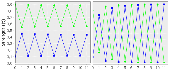
Figure 2. Divergence of QE(1) (left) and DFQ(1) (right) for $\mathcal{\textbf{A}}(1,0.9,0.1)$.

Since $\mathcal{\textbf{A}}(1,0.9,0.1)$ has indegree $2$, this is a tight example for DFQ(1) and QE(1) that shows that the general bounds given in Corollary 3 cannot be improved significantly.

As we illustrate in Figure 3, we can solve the divergence problem by increasing the conservativeness parameter $\kappa$ of the semantics. Indeed, since increasing the conservativeness decreases the Lipschitz-constant, we can see from Proposition 3 that the convergence guarantees improve. However, of course, this also affects the semantics as we discuss next.

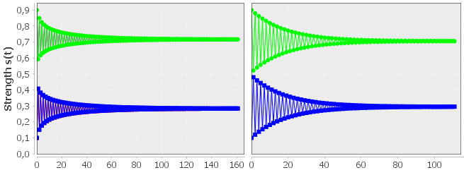
Figure 3. Convergence of QE($2.1$) (left) and DFQ($1.9$) (right) for $\mathcal{\textbf{A}}(1,0.9,0.1)$.

Open-Mindedness

Proposition 3 implies that semantics that use top for aggregation and an influence function with derivative bounded from above strictly by $\frac{1}{2}$ are guaranteed to converge. Hence, when using the Euler-based influence function or influence functions that scale the influence of the aggregated value down by a constant $\kappa$ similar to Linear($\kappa$) and p-Max($\kappa$), the semantics converges in general. While this is a nice guarantee, it does not come without cost. The bound imposed on the growth of the influence function limits the semantics’ ability to adapt the initial weight as we illustrate in the following example.

Example

Consider a BAG with one argument $a$ and $k$ arguments $b_{i}$ that attack $a$. All arguments have initial weight $0.9$. Table 3 shows final strength values of argument $a$ for modular semantics with different building blocks. Naturally, when using top for aggregation, the final strength is independent of the number of attackers. We can also see that increasing the conservativeness parameter lets the final strength values keep closer to the initial weights. Note also that the Euler-based semantics is extremely conservative.

$\alpha$	$\iota$	$k=1$	$k=10$	$k=100$
Sum	Euler	0.862	0.811	0.811
Top	Euler	0.862	0.862	0.862
Sum	2-Max(1)	0.498	0.012	0.001
Top	2-Max(1)	0.498	0.498	0.498
Sum	2-Max(5)	0.873	0.213	0.004
Top	2-Max(5)	0.873	0.873	0.873

Table 3. Strength values of $a$ under different semantics and increasing number of attackers $k$ for BAG from Example 3.

Arguably, a semantics should be able to move the strength values arbitrarily close to the extreme values $0$ or $1$ if sufficient evidence against or for the argument is given. We call such a semantics open-minded.

Definition (Open-Mindedness).

We say that an influence function $\iota:[l,u]\rightarrow[0,1]$ is open-minded if $\lim_{a\rightarrow l}\iota(a)=0$ and $\lim_{a\rightarrow u}\iota(a)=1$.

We call a basic modular semantics with aggregation function $\alpha:[0,1]^{n}\rightarrow[l,u]$ open-minded when its influence function restricted to the domain $[l,u]$ is open-minded.

Note that we do not demand that the influence function ever yields the extreme values $0$ or $1$ (this would be in conflict with the Resilience axiom from Amgoud and Ben-Naim (2017)), we only demand that it is possible to get arbitrarily close to these bounds. For the Euler-based influence function, we have $\lim_{a\rightarrow-\infty}\iota^{e}_{\mathcal{\operatorname{w}}}(a)=1-\frac{1-\mathcal{\operatorname{w}}^{2}}{1+\mathcal{\operatorname{w}}\cdot 0}=\mathcal{\operatorname{w}}^{2}$. Hence, the Euler-based semantics is not open-minded since it does not admit final strength values smaller than $\mathcal{\operatorname{w}}^{2}$. For example, in Table 3, the Euler-based influence function cannot yield a final strength value smaller than $0.9^{2}=0.81$. Linear($\kappa$) and p-Max($\kappa$) are open-minded influence functions and DFQ(1) and QE($\kappa$) are open-minded semantics. However, DFQ($\kappa$) is not open-minded for $\kappa>1$. Also, none of the semantics with general convergence guarantees from Mossakowski and Neuhaus (2018) are open-minded. These negative results are all special cases of the following proposition.

Proposition

Consider a basic modular semantics with aggregation function $\alpha:[0,1]^{n}\rightarrow[-B,B]$ and influence function $\iota$ whose Lipschitz constant is bounded by $\lambda^{\iota}$. Then for every BAG $\mathcal{\textbf{A}}=(\mathcal{A},\mathcal{\operatorname{w}},\mathcal{R},\mathcal{S})$ with $n$ arguments, the following bound is true for all $i=1,\dots,n$:

$$\mathcal{\operatorname{w}}_{i}-B\cdot\lambda^{\iota}\leq\operatorname{Deg}_{S}(\mathcal{\textbf{A}})_{i}\leq\mathcal{\operatorname{w}}_{i}+B\cdot\lambda^{\iota}.$$

Proof.

. By stability-$\iota$, we have $\iota_{\mathcal{\operatorname{w}}}(0)=\mathcal{\operatorname{w}}$. Hence, for all $a\in[-B,B]$, we have $|\iota_{\mathcal{\operatorname{w}}}(a)-\mathcal{\operatorname{w}}|=|\iota_{\mathcal{\operatorname{w}}}(a)-\iota_{\mathcal{\operatorname{w}}}(0)|\leq\lambda^{\iota}\cdot|a-0|\leq\lambda^{\iota}\cdot B.$ ∎

For example, the Euler-based influence function has $\lambda^{e}=0.25$. For aggregation with top, we have $B=1$. Hence, when combining these two, no weight can change by more than $0.25$.

It seems that when strong convergence guarantees can be derived from the contraction principle, they are bought at the expense of open-mindedness. The extreme case would be the constant influence function $\iota_{\mathcal{\operatorname{w}}}(a)=\mathcal{\operatorname{w}}$ that just assigns the initial weight to every aggregate. Its Lipschitz constant is $0$ and every basic modular semantics that uses this influence function is guaranteed to converge trivially. As we let $\kappa$ in DFQ($\kappa$) and QE($\kappa$) go to infinity, we gradually increase our convergence guarantees, but simultaneously approach the constant influence function that leaves all weights unchanged. All currently known convergence guarantees for cyclic BAGs seem to be of this kind: we buy convergence guarantees at the expense of open-mindedness.

4. Continuous Modular Semantics

We now look at another approach to improve convergence guarantees. Instead of making semantics more conservative, we will adapt the update approach. Roughly speaking, we will replace coarse updates with more fine-grained updates. We will show that this approach leaves the semantics unchanged in cases where we have convergence guarantees. More importantly, it can still converge to a fixed-point of the semantics when the original updating approach diverges.

Roughly speaking, discrete update approaches work by applying an update formula to the initial weights repeatedly until the process converges. In case of basic modular semantics, the update formula is given by the function $(\iota_{\mathcal{\operatorname{w}}_{i}}\circ\alpha_{g_{i}})$. In Potyka (2018a), it has been proposed to use continuous models rather than discrete ones in order to deal with cyclic BAGs. Continuous models can be designed in a more descriptive way than discrete models. To this end, the continuous change of arguments’ strength based on the strength of their attackers and supporters is described by means of differential equations. If the system of differential equations is designed carefully, it yields a unique solution $\sigma^{\mathcal{\textbf{A}}}:\mathbb{R}^{+}_{0}\rightarrow\mathbb{R}^{n}$. Intuitively, the $i$-th component $\sigma^{\mathcal{\textbf{A}}}_{i}(t)$ tells us the strength of the $i$-th argument at (continuous) time $t$ and the final strength values correspond to the limit $\lim_{t\rightarrow\infty}\sigma^{\mathcal{\textbf{A}}}(t)$. Just like the limit $\lim_{k\rightarrow\infty}f_{S}^{k}(\mathcal{\operatorname{w}})$ for discrete basic modular semantics may not exist, the limit $\lim_{t\rightarrow\infty}\sigma^{\mathcal{\textbf{A}}}(t)$ may not exist. However, if we can continuize a discrete model, the discrete model can actually be seen as a coarse approximation of the continuous model Potyka (2018a). In particular, the continuous model may still converge when its discrete counterpart diverges as we will demonstrate soon. While there are currently no strong analytical guarantees for continuous models in cyclic BAGs, no divergence examples have been found either and experiments show that they can converge quickly for large cyclic BAGs with thousands of arguments. Furthermore, sufficient conditions have been given under which discrete models can be continuized. The results can actually be simplified and generalized to all basic modular semantics. The key property of the aggregation and influence functions is again Lipschitz continuity.

Before stating the result, we add some explanations. The continuized model can be obtained as the unique solution of a system of differential equations. The equations basically describe how the strength evolves at each current point in time based on the current strength. This is done by defining the derivatives of the function $\sigma^{\mathcal{\textbf{A}}}:\mathbb{R}^{+}_{0}\rightarrow\mathbb{R}^{n}$. As it turns out, in order to continuize a basic modular semantics, we can just define the derivative for the i-th strength value at time $t$ as the difference $(\iota_{\mathcal{\operatorname{w}}_{i}}\circ\alpha_{g_{i}})(\sigma(t))-\sigma_{i}(t)$. That is, as the difference between the result of applying the update function to the current state and the state itself. Note that the difference is $0$ if $\sigma(t)$ is a fixed-point of the function $(\iota_{\mathcal{\operatorname{w}}_{i}}\circ\alpha_{g_{i}})$. In this case, the strength value remains unchanged. If $(\iota_{\mathcal{\operatorname{w}}_{i}}\circ\alpha_{g_{i}})(\sigma(t))>\sigma_{i}(t)$, the difference, and hence the slope, will be positive and the strength value increases. This does again make intuitively sense because the strength will be shifted towards the strength value that is desired by the update formula. For the case $(\iota_{\mathcal{\operatorname{w}}_{i}}\circ\alpha_{g_{i}})(\sigma(t))<\sigma_{i}(t)$, the strength decreases symmetrically. We are now ready to state the general result. As usual, we leave out the function parameter $t$ when writing differential equations.

Proposition (Continuizing Basic Modular Semantics)

Let $\operatorname{Deg}_{S}$ be a basic modular semantics with aggregation function $\alpha_{g}$ and influence function $\iota_{w}$.

1. For all BAGs A, the system of differential equations

   $$\frac{\mathrm{d}\sigma_{i}}{\mathrm{d}t}=(\iota_{\mathcal{\operatorname{w}}_{i}}\circ\alpha_{g_{i}})(\sigma)-\sigma_{i}$$ (1)

   with initial conditions $\sigma_{i}(0)=\mathcal{\operatorname{w}}(i)$ for $i=1,\dots,n$ has a unique solution $\sigma^{\mathcal{\textbf{A}}}:\mathbb{R}^{+}_{0}\rightarrow\mathbb{R}^{n}$.

2. If $\sigma^{\mathcal{\textbf{A}}}$ converges and $s^{*}=\lim_{t\rightarrow\infty}\sigma^{\mathcal{\textbf{A}}}(t)$, then $s^{*}$ is a fixed-point of the update function $f_{S}$ of $\operatorname{Deg}_{S}$.

3. If A is acyclic, the discrete and continuized models converge to the same limit.

4. If $\sigma^{\mathcal{\textbf{A}}}$ converges and $f_{S}$ is a contraction, then the discrete and continuized models converge to the same limit.

Proof.

1. Lipschitz continuity of $(\iota_{\mathcal{\operatorname{w}}_{i}}\circ\alpha_{g_{i}})$ allows us to apply existence and uniqueness theorems for nonlinear systems of ordinary differential equations from (Polyanin and Zaitsev, 2017, Section 7.1.2) that imply the claim.

2. If $\sigma^{\mathcal{\textbf{A}}}$ converges, then all derivatives $\frac{\mathrm{d}\sigma_{i}}{\mathrm{d}t}$ must go to $0$. Hence, in the limit $0=(\iota_{\mathcal{\operatorname{w}}_{i}}\circ\alpha_{g_{i}})(s^{*})-s^{*}_{i}$. That is, $f_{i}(s^{*})=(\iota_{\mathcal{\operatorname{w}}_{i}}\circ\alpha_{g_{i}})(s^{*})=s^{*}_{i}$.

3. Analogous to the proof of Proposition 16 in Potyka (2018a), one can show that $\sigma^{\mathcal{\textbf{A}}}$ converges to the same limit as the algorithm given in Proposition 3 for acyclic BAGs.

4. If $f_{S}$ is a contraction, the contraction principle implies that $f_{S}$ has a unique fixed-point. Since $\sigma^{\mathcal{\textbf{A}}}$ converges to such a fixed-point according to Item 2, both models must converge to the same limit. ∎

As opposed to the continuization result in Potyka (2018a), the proposition does not assume continuous differentiability of the update function and therefore applies to more general acceptability semantics like the DF-QuAD algorithm from Rago et al. (2016) (DFQ(1) in Table 2). The reason that the result applies to all basic modular semantics is that they have a Lipschitz-continuous update function, which is sufficient.

We demonstrate in Figure 4 that continuizing discrete models can solve divergence problems. Whereas QE(1) and DFQ(1) diverged for $\mathcal{\textbf{A}}(1,0.9,0.1)$ (Figure 2), their continuized counterparts (Figure 4) converge.

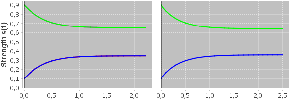
Figure 4. Convergence of Continuous QE(1) (left) and Continuous DFQ(1) (right) for $\mathcal{\textbf{A}}(1,0.9,0.1)$.

The intuitive reason for this is best explained by numerical solution techniques that approximate the continuous model $\sigma^{\mathcal{\textbf{A}}}:\mathbb{R}^{+}_{0}\rightarrow\mathbb{R}^{n}$. The most naive technique is Euler’s method. In our context, it initializes the strength values with the initial conditions given by the initial weights. That is, $\sigma^{\mathcal{\textbf{A}}}(0)=\mathcal{\operatorname{w}}$. In order to compute $\sigma^{\mathcal{\textbf{A}}}(\delta)$ for some small $\delta>0$, Euler’s method uses a first-order Taylor approximation. The first order Taylor approximation of a differentiable function $f:\mathbb{R}\rightarrow\mathbb{R}^{n}$ about a point $t$ is given as $f_{i}(t+\delta)\approx f_{i}(t)+\delta\cdot\frac{\mathrm{d}f_{i}}{\mathrm{d}t}(t)$. Since we know $\sigma^{\mathcal{\textbf{A}}}(0)=\mathcal{\operatorname{w}}$ and $\frac{\mathrm{d}\sigma^{\mathcal{\textbf{A}}}_{i}}{\mathrm{d}t}(0)=(\iota_{\mathcal{\operatorname{w}}_{i}}\circ\alpha_{g_{i}})(\mathcal{\operatorname{w}})-\mathcal{\operatorname{w}}$, the first-order Taylor approximation of $\sigma^{\mathcal{\textbf{A}}}_{i}(\delta)$ is $\mathcal{\operatorname{w}}+\delta\cdot\big{(}(\iota_{\mathcal{\operatorname{w}}_{i}}\circ\alpha_{g_{i}})(\mathcal{\operatorname{w}})-\mathcal{\operatorname{w}}\big{)}$. Having obtained our approximation for $\sigma^{\mathcal{\textbf{A}}}(\delta)$, we can move on approximating $\sigma^{\mathcal{\textbf{A}}}(2\cdot\delta)$ analogously. In this way, we can approximate $\sigma^{\mathcal{\textbf{A}}}(t)$ for all $t>0$ until the strength values converge. $\delta$ is called the step-size of the approximation and we can improve the approximation quality by decreasing $\delta$. As $\delta\rightarrow 0$, the approximation error goes to $0$ by differentiability of $\sigma^{\mathcal{\textbf{A}}}$.

Interestingly, the discrete update scheme turns out to be a Taylor-approximation of the continuous model with step size $1$. To see this, just plug in $\delta=1$ in our formula above. Then the approximation of $\sigma^{\mathcal{\textbf{A}}}(1)$ is $\mathcal{\operatorname{w}}+1\cdot\big{(}(\iota_{\mathcal{\operatorname{w}}_{i}}\circ\alpha_{g_{i}})(\mathcal{\operatorname{w}})-\mathcal{\operatorname{w}}\big{)}=(\iota_{\mathcal{\operatorname{w}}_{i}}\circ\alpha_{g_{i}})(\mathcal{\operatorname{w}})$. Notice that this is just our update formula applied to the initial weights once. Hence, applying the update formula once can be seen as a very coarse approximation of the continuous model at time $1$ and, more generally, applying the update formula $k$ times can be seen as a coarse approximation of the continuous model at time $k$. Due to this coarseness, we may actually jump from the function graph of the true solution to the function graph of a solution for different initial conditions. This may cause divergence when the algorithm starts jumping back and forth between two function graphs. We can avoid these jumps by decreasing $\delta$. We illustrate this in Figure 5 for DFQ(1) and the BAG $\mathcal{\textbf{A}}(1,0.9,0.1)$. As we decrease $\delta$ from $1$ to $0.8$, the oscillations already become weaker, but the step size is not sufficiently small to avoid divergence. For $\delta=0.5$, the oscillations die out and the true limit shown in Figure 4 is eventually reached.

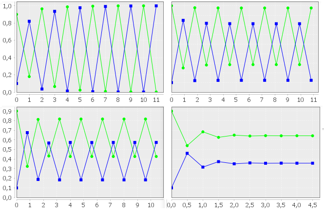
Figure 5. Approximating Continuous DFQ(1) with Euler’s method for $\mathcal{\textbf{A}}(1,0.9,0.1)$ with $\delta=1$ (upper left), $\delta=0.9$ (upper right), $\delta=0.8$ (lower left) and $\delta=0.5$ (lower right)

Of course, we refer to Euler’s method only for didactic reasons. The results in Figure 4 were computed using the classical Runge-Kutta method RK4 that provides much stronger approximation guarantees Polyanin and Zaitsev (2017).

5. Duality Property

In order to complement the semantical properties of basic modular semantics, we now generalize a symmetry property introduced in Potyka (2018a) to the setting from Mossakowski and Neuhaus (2018). Intuitively, our symmetry property should assure that attackers move the strength from the initial weight towards $0$ in the same way as supporters move the strength from the initial weight towards $1$. This can be described by constraints on the aggregation and influence functions as follows.

Definition (Duality).

A basic modular semantics satisfies Duality iff

1. $\alpha_{g}(s)=-\alpha_{-g}(s)$ for all $s\in[0,1]^{n}$ and

2. $1-\iota_{(1-\mathcal{\operatorname{w}})}(a)=\iota_{\mathcal{\operatorname{w}}}(-a)$ for all $\mathcal{\operatorname{w}}\in[0,1]$.

The aggregation condition says that when we switch the role of attackers and supporters (replace $g$ with $-g$), the aggregated strength value should just switch sign. For the special case $\mathcal{\operatorname{w}}=0.5$, the influence condition says that a positive aggregate must yield the same distance to $1$ as the negative aggregate yields to $0$. If $\mathcal{\operatorname{w}}\neq 0.5$, there is a natural asymmetry because the initial weight is now either closer to $0$ or $1$. However, a negative aggregate for weight $w$ should still yield the same distance to $0$ as the positive aggregate yields to $1$ for weight $1-w$. In the following proposition, we give a more intuitive interpretation of Duality.

Proposition

Let $\operatorname{Deg}_{S}$ be a basic modular semantics that satisfies Duality and let $\mathcal{\textbf{A}}=(\mathcal{A},\mathcal{\operatorname{w}},\mathcal{R},\mathcal{S})$ be a BAG such that $\operatorname{Deg}_{S}(\mathcal{\textbf{A}})=s^{*}\neq\bot$. If there are $\mathcal{A}_{i},\mathcal{A}_{j}$ such that

1. $g_{i}=-g_{j}$ or, more generally, $\alpha_{g_{i}}(s^{*})=-\alpha_{g_{j}}(s^{*})$,

2. $\mathcal{\operatorname{w}}_{i}=1-\mathcal{\operatorname{w}}_{j}$,

then $\operatorname{Deg}_{S}(\mathcal{\textbf{A}})_{i}=1-\operatorname{Deg}_{S}(\mathcal{\textbf{A}})_{j}$.

Proof.

First note that $g_{i}=-g_{j}$ implies $\alpha_{g_{i}}(s^{*})=\alpha_{-g_{i}}(s^{*})=-\alpha_{g_{j}}(s^{*})$ by Duality of the aggregation function. By the contraction principle, $s^{*}$ is a fixed-point of $(\iota_{\mathcal{\operatorname{w}}_{i}}\circ\alpha_{g_{i}})$ and $(\iota_{\mathcal{\operatorname{w}}_{j}}\circ\alpha_{g_{j}})$. Therefore,

$$s_{i}^{*} =\iota_{\mathcal{\operatorname{w}}_{i}}(\alpha_{g_{i}}(s^{*}))=\iota_{\mathcal{\operatorname{w}}_{i}}(-\alpha_{g_{j}}(s^{*}))=1-\iota_{\mathcal{\operatorname{w}}_{j}}(\alpha_{g_{j}}(s^{*}))$$

$$=1-s_{j}^{*}.$$

∎

The basic case of the first condition says that $\mathcal{A}_{i}$’s attackers are $\mathcal{A}_{j}$’s supporters and vice versa. This is intuitive, but somewhat restrictive. The more general version says that the magnitude of the aggregated strength at $\mathcal{A}_{i}$ and $\mathcal{A}_{j}$ is equal, but it acts in different directions. The second condition says that the initial weights of $\mathcal{A}_{i}$ and $\mathcal{A}_{j}$ are complementary. Intuitively, we should then expect that their final strength values will also be complementary. We illustrate this in the following example.

Example

Consider the BAG in Figure 6.

Figure 6. Duality Example.

Table 4 shows the strength values for the three semantics from Table 2.

	$a_{1}$	$b_{1}$	$a_{2}$	$b_{2}$	$a_{3}$	$b_{3}$
Weight $\mathcal{\operatorname{w}}$	$0.50$	$0.50$	$0.70$	$0.30$	$0.20$	0.80
Euler	$0.39$	$0.65$	$0.63$	$0.41$	$0.15$	$0.84$
DFQ(1)	$0.10$	$0.90$	$0.28$	$0.72$	$0.12$	$0.88$
QE(1)	$0.30$	$0.70$	$0.51$	$0.49$	$0.17$	$0.83$

Table 4. Initial weight and strength values for arguments in Figure 6 under semantics from Table 2.

The asymmetry of the Euler-based semantics can already be seen from the subgraph with indices $1$. Whereas the support of $x_{1}$ increases the strength of $b_{1}$ by $0.15$, its attack decreases the strength of $a_{1}$ only by $0.11$. Both the DF-QuAD algorithm and the quadratic energy model induce a symmetrical impact for attacks and supports.

As we move the initial weight away from $0.5$, there is a natural asymmetry caused by the fact that the distance from the initial weight to $0$ and $1$ is now different. However, attack and support should still behave in a dual manner. For the subgraph with indices $2$, the initial weight of $a_{2}$ and $b_{2}$ is moved away from $0.5$ by $0.2$ in different directions. Again, the increase caused by a support should equal the decrease caused by an attack. For the DF-QuAD algorithm, the change is $0.42$, for the quadratic energy model $0.19$. Similarly, for the subgraph with indices $3$, the DF-QuAD algorithm causes a change of $0.08$, the quadratic energy model causes a change of $0.03$.

In Table 1, all building blocks other than the Euler-based influence functions can be selected in order to satisfy duality as we show in the following proposition.

Proposition

The Sum-, Product- and Top-aggregation functions satisfy condition 1 in Definition 5. The Linear($\kappa$) and p-Max($\kappa$) influence functions satisfy condition 2 in Definition 5.

Proof.

Sum:

$$\alpha^{\Sigma}_{g}(s)=\sum_{i}g_{i}\cdot s_{i}=-\sum_{i}(-g_{i})\cdot s_{i}=-\alpha^{\Sigma}_{-g}(s).$$

Product:

$$\alpha^{\Pi}_{g}(s) =\prod_{i:g_{i}=-1}(1-s_{i})-\prod_{i:g_{i}=1}^{n}(1-s_{i})$$

$$=-\big{(}-\prod_{i:-g_{i}=1}(1-s_{i})+\prod_{i:-g_{i}=-1}^{n}(1-s_{i})\big{)}$$

$$=-\alpha^{\Pi}_{-g}(s).$$

Top:

$$\alpha^{\textit{max}}_{g}(s) =M_{g}(s)-M_{-g}(s)=-(-M_{g}(s)+M_{-g}(s))$$

$$=-\alpha^{\textit{max}}_{-g}(s).$$

Linear($\kappa$):

$$1-\iota^{l}_{(1-\mathcal{\operatorname{w}})}(a)$$

$$=\mathcal{\operatorname{w}}+\frac{1-\mathcal{\operatorname{w}}}{\kappa}\cdot\max\{0,-a\}-\frac{\mathcal{\operatorname{w}}}{\kappa}\cdot\max\{0,a\}$$

$$=\iota^{l}_{\mathcal{\operatorname{w}}}(-a).$$

p-Max($\kappa$):

$$1-\iota^{p}_{(1-\mathcal{\operatorname{w}})}(a)$$

$$=\mathcal{\operatorname{w}}+\frac{1-\mathcal{\operatorname{w}}}{\kappa}\cdot h(-a)-\frac{\mathcal{\operatorname{w}}}{\kappa}\cdot h(a)$$

$$=\iota^{p}_{\mathcal{\operatorname{w}}}(-a).$$

∎

Since the DF-QuAD algorithm and the quadratic energy model are constructed from these building blocks, an immediate consequence is that they satisfy duality.

6. Implementing Modular Semantics with Attractor

The framework of modular semantics and has been implemented in the Java library Attractor Potyka (2018b). The user can initialize modular semantics with different combinations of aggregation and influence functions and can use existing implementations of algorithms to compute strength values using discrete (by using Euler’s method with step size $1$) or continuous semantics. Implementations of the aggregation and influence functions discussed here already exist, but new functions can be added easily by implementing existing interfaces. For example, the semantics of the DF-QuAD algorithm can be initialized with the following three lines of code:

AggregationFunction agg = new ProductAggregation();

InfluenceFunction inf = new LinearInfluence(1);

ContinuousModularModel mod =

new ContinuousModularModel(agg, inf);

Attractor contains implementations of RK4 (for reliable computations) and Euler’s method (for simulating discrete semantics and illustration purposes). Both implementations have a printing variant that automatically generates plots like in Figure 4 (RK4) and Figure 2 (Euler) while computing the solution. The plots are generated by JFreeChart. For example, in order to use the plotting variant of RK4, we can add the following code:

AbstractIterativeApproximator approximator =

new PlottingRK4(mod);

mod.setApproximator(approximator);

Finally, the strength values for a BAG can be computed. Attractor provides a simple syntax to define BAGs in text files. The file format is inspired by the format used in ConArg Bistarelli et al. (2016), but adds weights and support relations. BAGs can also be defined programmatically if more flexibility is required. We refer to Potyka (2018b) for details on creating BAGs. Assuming that a BAG file is given, the strength values can be computed by adding the following lines of code:

BAGFileUtils fileUtils = new BAGFileUtils();

BAG bag = fileUtils.readBAGFromFile(file);

mod.setBag(bag);

mod.approximateSolution(10e-2, 10e-4, true);

The two numerical parameters correspond to the step size and the termination condition, respectively. Mathematically, the algorithms converge to a fixed-point at which all derivatives will be $0$. However, even mathematically, the fixed-point may not be reached in finite time. In practice, we also have to think about numerical accuracy, and so we usually stop when the derivatives are sufficiently small. Let us emphasize that the user does not have to think about derivatives. The derivatives are given by the differential equations. When adding new aggregation or influence functions, the differential equations are automatically derived as explained in Proposition 4. The logic is already implemented in the class ContinuousModularModel. So when implementing a new aggregation or influence function, only the logic for aggregating strength values or adapting the initial weight needs to be implemented.

7. Related Work

In the original abstract argumentation framework Dung (1995), arguments can only be attacked by other arguments. Bipolar argumentation frameworks Amgoud et al. (2004); Oren and Norman (2008); Cayrol and Lagasquie-Schiex (2013) add a support relation. Classical semantics can only accept or reject arguments Baroni et al. (2011), but various proposals have been made to allow for a more fine-grained evaluation. Among others, it has been suggested to apply tools from probabilistic reasoning Dung and Thang (2010); Li et al. (2011); Rienstra (2012); Hunter (2014); Doder and Woltran (2014); Polberg and Doder (2014); Hunter and Thimm (2014); Prakken (2018); Hunter et al. (2018); Rienstra et al. (2018) or to rank arguments based on fixed-point equations Besnard and Hunter (2001); Leite and Martins (2011); Correia et al. (2014); Barringer et al. (2012) or the graph structure Cayrol and Lagasquie-Schiex (2005); Amgoud and Ben-Naim (2013).

In recent years, several weighted bipolar argumentation frameworks as considered here have been presented Baroni et al. (2015); Rago et al. (2016); Amgoud and Ben-Naim (2017); Mossakowski and Neuhaus (2018); Potyka (2018a). The QuAD algorithm from Baroni et al. (2015) was designed to evaluate the strength of answers in decision-support systems. However, it can show discontinuous behaviour that is undesirable in some cases. The DF-QuAD algorithm (Discontinuity-free QuAD) Rago et al. (2016) was proposed as an alternative that avoids this behaviour. Some additional interesting semantical guarantees are given by the Euler-based semantics that was introduced in Amgoud and Ben-Naim (2017). The QuAD algorithms mainly lack these properties due to the fact that their aggregated strength values saturate. That is, as soon, as an attacker (supporter) with strength $1$ exists, the other attackers (supporters) become irrelevant for the aggregated value. The Euler-based semantics avoids many problems, but has some other drawbacks that can be undesirable. Arguments initialized with strength $0$ or $1$ remain necessarily unchanged under Euler-based semantics and, as we saw, attacks and supports have an asymmetrical impact. The quadratic energy model introduced in Potyka (2018a) avoids these problems. In Mossakowski and Neuhaus (2018), some other related models have been studied that use initial weights, an aggregation and an influence function as well, but the final strength values can also take values from the interval $[-1,1]$ or general real numbers. Other aggregation and influence functions for these cases have been discussed in Mossakowski and Neuhaus (2018) as well.

A first collection of general axioms for weighted bipolar frameworks has been presented in Amgoud and Ben-Naim (2017). Several authors noted recently that the axioms can be simplified by using more elementary properties Mossakowski and Neuhaus (2018); Baroni et al. (2018); Amgoud and Doder (2018). The idea of modular semantics from Mossakowski and Neuhaus (2018) seems particularly useful because it allows creating new semantics with interesting guarantees by simply combining suitable aggregation and influence functions. This approach bears some resemblance to representation theorems considered in other fields that relate semantical properties of operators to elementary properties of functions that can be used to create these operators. Some ideas similar to modular semantics have been invented independently for the special case where only attack relations are present in Amgoud and Doder (2018).

8. Discussion and Future Work

We extended the framework of modular semantics from Mossakowski and Neuhaus (2018) in several directions. Our main focus was on convergence guarantees. We generalized the convergence guarantees from Mossakowski and Neuhaus (2018) to Lipschitz-continuous aggregation and influence functions. This allowed us, in particular, to derive convergence guarantees for semantics based on product-aggregation like the DF-QuAD algorithm. We also complemented the results from Mossakowski and Neuhaus (2018) with runtime guarantees based on the approximation accuracy and the Lipschitz constants. The Lipschitz constants provided in Table 1 can be used to derive further convergence guarantees in combination with Proposition 3. There are many other interesting candidates for aggregation and influence functions and, provided that they are Lipschitz-continuous, Proposition 3 can be applied to derive convergence guarantees easily. For example, truncated sums like the Lukasiewicz T-conorm could be interesting. In combination with the linear influence function they can guarantee that the extreme values $0$ and $1$ are taken in desirable cases (e.g., if there is only one attacker/supporter with strength $1$) while avoiding the saturation property of the QUAD algorithms.

As we discussed, convergence guarantees for discrete models are often bought at the expense of open-mindedness. We demonstrated that we can avoid divergence problems without giving up open-mindedness by continuizing discrete models as proposed in Potyka (2018a). It is currently an open question if and under which conditions continuous models converge for general cyclic BAGs, but until now, no divergence examples have been found. The continuization of all basic modular semantics yields a well-defined continuous model as Proposition 4 explains. The limits of discrete and continuized models are guaranteed to be equal for acyclic BAGs and for cyclic BAGs that induce a contractive update function. Further investigations are necessary, but it currently seems that whenever a discrete model converges, the continuized model converges to the same solution.

Semantically, we complemented modular semantics with the Duality property. After relating this property to elementary properties of aggregation and influence functions, it can be checked more easily. We showed, in particular, that it is satisfied by DF-QuAD.

Finally, we explained how weighted argumentation problems can be solved with the Java library Attractor. Modular semantics allow for very convenient abstractions. Dependent on the user’s expertise, new semantics can be implemented completely from scratch, can be constructed from self-implemented aggregation and influence functions or by just combining pre-implemented aggregation and influence functions. A graphical user interface is work in progress.

References

- (1)
- Alsinet et al. (2017) Teresa Alsinet, Josep Argelich, Ramón Béjar, Cèsar Fernández, Carles Mateu, and Jordi Planes. 2017. Weighted argumentation for analysis of discussions in Twitter. International Journal of Approximate Reasoning 85 (2017), 21–35.
- Amgoud and Ben-Naim (2013) Leila Amgoud and Jonathan Ben-Naim. 2013. Ranking-based semantics for argumentation frameworks. In International Conference on Scalable Uncertainty Management (SUM). Springer, 134–147.
- Amgoud and Ben-Naim (2016a) Leila Amgoud and Jonathan Ben-Naim. 2016a. Axiomatic Foundations of Acceptability Semantics. In International Conference on Principles of Knowledge Representation and Reasoning (KR). 2–11.
- Amgoud and Ben-Naim (2016b) Leila Amgoud and Jonathan Ben-Naim. 2016b. Evaluation of arguments from support relations: Axioms and semantics. In International Joint Conferences on Artificial Intelligence (IJCAI). pp–900.
- Amgoud and Ben-Naim (2017) Leila Amgoud and Jonathan Ben-Naim. 2017. Evaluation of arguments in weighted bipolar graphs. In European Conference on Symbolic and Quantitative Approaches to Reasoning with Uncertainty (ECSQARU). Springer, 25–35.
- Amgoud et al. (2004) Leila Amgoud, Claudette Cayrol, and Marie-Christine Lagasquie-Schiex. 2004. On the bipolarity in argumentation frameworks. In International Workshop on Non-Monotonic Reasoning (NMR), Vol. 4. 1–9.
- Amgoud and Doder (2018) Leila Amgoud and Dragan Doder. 2018. Gradual Semantics for Weighted Graphs: An Unifying Approach. In International Conference on Principles of Knowledge Representation and Reasoning (KR). 613–614.
- Baroni et al. (2011) Pietro Baroni, Martin Caminada, and Massimiliano Giacomin. 2011. An introduction to argumentation semantics. The Knowledge Engineering Review 26, 4 (2011), 365–410.
- Baroni et al. (2018) Pietro Baroni, Antonio Rago, and Francesca Toni. 2018. How many properties do we need for gradual argumentation?. In AAAI Conference on Artificial Intelligence (AAAI). AAAI, 1736–1743.
- Baroni et al. (2013) Pietro Baroni, Marco Romano, Francesca Toni, Marco Aurisicchio, and Giorgio Bertanza. 2013. An argumentation-based approach for automatic evaluation of design debates. In International Workshop on Computational Logic in Multi-Agent Systems. Springer, 340–356.
- Baroni et al. (2015) Pietro Baroni, Marco Romano, Francesca Toni, Marco Aurisicchio, and Giorgio Bertanza. 2015. Automatic evaluation of design alternatives with quantitative argumentation. Argument & Computation 6, 1 (2015), 24–49.
- Barringer et al. (2012) Howard Barringer, Dov M Gabbay, and John Woods. 2012. Temporal, numerical and meta-level dynamics in argumentation networks. Argument & Computation 3, 2-3 (2012), 143–202.
- Besnard and Hunter (2001) Philippe Besnard and Anthony Hunter. 2001. A logic-based theory of deductive arguments. Artificial Intelligence 128, 1-2 (2001), 203–235.
- Bistarelli et al. (2016) Stefano Bistarelli, Fabio Rossi, and Francesco Santini. 2016. ConArg: A Tool for Classical and Weighted Argumentation. In International Conference on Computational Models of Argument (COMMA). 463–464.
- Cayrol and Lagasquie-Schiex (2005) Claudette Cayrol and Marie-Christine Lagasquie-Schiex. 2005. Graduality in Argumentation. Journal of Artificial Intelligence Research 23 (2005), 245–297.
- Cayrol and Lagasquie-Schiex (2013) Claudette Cayrol and Marie-Christine Lagasquie-Schiex. 2013. Bipolarity in argumentation graphs: Towards a better understanding. International Journal of Approximate Reasoning 54, 7 (2013), 876–899.
- Cormen et al. (2009) Thomas H Cormen, Charles E Leiserson, Ronald L Rivest, and Clifford Stein. 2009. Introduction to Algorithms. MIT Press, Cambridge, Massachusetts.
- Correia et al. (2014) Marco Correia, Jorge Cruz, and Joao Leite. 2014. On the Efficient Implementation of Social Abstract Argumentation. In European Conference on Artificial Intelligence (ECAI). 225–230.
- Doder and Woltran (2014) Dragan Doder and Stefan Woltran. 2014. Probabilistic argumentation frameworks–a logical approach. In International Conference on Scalable Uncertainty Management (SUM). Springer, 134–147.
- Dung (1995) Phan Minh Dung. 1995. On the acceptability of arguments and its fundamental role in nonmonotonic reasoning, logic programming and n-person games. Artificial intelligence 77, 2 (1995), 321–357.
- Dung and Thang (2010) Phan Minh Dung and Phan Minh Thang. 2010. Towards (probabilistic) argumentation for jury-based dispute resolution. International Conference on Computational Models of Argument (COMMA) 216 (2010), 171–182.
- Hunter (2014) Anthony Hunter. 2014. Probabilistic qualification of attack in abstract argumentation. International Journal of Approximate Reasoning 55, 2 (2014), 607–638.
- Hunter et al. (2018) Anthony Hunter, Sylwia Polberg, and Nico Potyka. 2018. Updating Belief in Arguments in Epistemic Graphs. In International Conference on Principles of Knowledge Representation and Reasoning (KR). 138–147.
- Hunter and Thimm (2014) Anthony Hunter and Matthias Thimm. 2014. Probabilistic argumentation with incomplete information. In European Conference on Artificial Intelligence (ECAI). IOS Press, 1033–1034.
- Leite and Martins (2011) Joao Leite and Joao Martins. 2011. Social abstract argumentation. In International Joint Conferences on Artificial Intelligence (IJCAI), Vol. 11. 2287–2292.
- Li et al. (2011) Hengfei Li, Nir Oren, and Timothy J Norman. 2011. Probabilistic argumentation frameworks. In International Workshop on Theory and Applications of Formal Argumentation. Springer, 1–16.