Submillimeter Polarization Spectrum of the Carina Nebula

Abstract

Linear polarization maps of the Carina Nebula were obtained at 250, 350, and 500 $\mathrm{\SIUnitSymbolMicro m}$ during the 2012 flight of the BLASTPol balloon-borne telescope. These measurements are combined with Planck 850 $\mathrm{\SIUnitSymbolMicro m}$ data in order to produce a submillimeter spectrum of the polarization fraction of the dust emission, averaged over the cloud. This spectrum is flat to within $\pm$15% (relative to the 350 $\mathrm{\SIUnitSymbolMicro m}$ polarization fraction). In particular, there is no evidence for a pronounced minimum of the spectrum near 350 $\mathrm{\SIUnitSymbolMicro m}$, as suggested by previous ground-based measurements of other molecular clouds. This result of a flat polarization spectrum in Carina is consistent with recently-published BLASTPol measurements of the Vela C molecular cloud, and also agrees with a published model for an externally-illuminated, dense molecular cloud by Bethell and collaborators. The shape of the spectrum in Carina does not show any dependence on the radiative environment of the dust, as quantified by the Planck-derived dust temperature or dust optical depth at 353 GHz.

1. Introduction

Dust grains in the interstellar medium (ISM) have long been known to linearly polarize background starlight at visible and near-infrared wavelengths (Hall, 1949; Hiltner, 1949). The thermal emission from these dust grains in the far-infrared and submillimeter portion of the spectrum is observed to be linearly polarized as well (Cudlip et al., 1982; Hildebrand et al., 1984). It is believed that the aspherical, spinning dust grains align with their long axes perpendicular to the direction of the local ISM magnetic field. The mechanism for the alignment of the dust grains is an area of active research, but recently the theory of radiative alignment torques (RATs) has gained some observational support. Under the RAT mechanism (Lazarian & Hoang, 2007), an external radiation field is able to provide a net torque to spin up dust grains, which develop a net magnetic dipole moment that aligns with the direction of the local magnetic field. A detailed review is given in Andersson et al. (2015). In particular, they note that RAT alignment requires the presence of a radiation field with wavelengths less than the grain diameter. This condition predicts a lower alignment efficiency, and hence a lower polarization fraction, with increasing dust extinction.

The aligned dust grains preferentially absorb and emit light that is polarized in the direction parallel to their long axes. As a result, transmitted starlight is preferentially polarized in the direction parallel to the local magnetic field, whereas the dust thermal emission is polarized in the direction perpendicular to the magnetic field. Dust polarimetry therefore allows the directions of the plane-of-sky projection of the ISM magnetic field to be traced. This measurement can serve as a powerful tool for investigating the role played by magnetic fields in the early stages of star formation. This is true particularly when the polarization is measured in emission at longer wavelengths, where it can be traced into the interiors of the dense clouds of molecular gas where star formation takes place. Measurements of polarized dust emission in the diffuse ISM are also important, since this emission is a source of foreground contamination to studies of the polarization of the Cosmic Microwave Background (CMB) radiation. Data that provide a better understanding of the variation of the dust polarization fraction with wavelength, and with dust environment are important to both of these scientific applications.

The submillimeter polarization spectrum $p(\lambda)$ is the linear polarization fraction of the thermal dust emission as a function of wavelength (polarization fraction being defined in Section 2.5). Typically, the spectrum is divided by the polarization fraction at a reference wavelength $\lambda_{0}$. This normalization removes the dependence on the inclination angle of the magnetic field relative to the line of sight, and on any other unknown factors that would affect the observed polarization fraction across all bands. The relevant observable for the study of dust grain alignment is then the shape of this normalized spectrum $p(\lambda)/p(\lambda_{0})$.

A number of models have been developed attempting to predict the shape of the polarization spectrum over the submillimeter spectrum, in various column density regimes. Draine & Fraisse (2009) investigated the polarization of dust in the diffuse ISM using models of aspherical silicate and graphite grains that were constrained to reproduce the observed dust extinction and polarization of starlight as a function of wavelength. They produced model polarization spectra that were rising from 100 $\mathrm{\SIUnitSymbolMicro m}$ to 1000 $\mathrm{\SIUnitSymbolMicro m}$. For a scenario in which the dust is diffuse enough that all grains are exposed to the same interstellar radiation field, it is not unreasonable to assume that the dust temperature will depend only on grain material and size, and not on physical location. Under this assumption, the rising spectrum can be explained, at least in part, in terms of an anti-correlation between dust temperature and grain alignment. Larger dust grains are known empirically to be better-aligned (Kim & Martin, 1995). However, larger dust grains also have higher emissivity and thus tend towards lower equilibrium temperatures. Therefore, it is the well-aligned lower-temperature grains, whose emission peaks at longer wavelengths, that contribute predominantly to the polarization fraction in this scenario.

In contrast to this diffuse ISM study, Bethell et al. (2007) modelled polarized dust emission in dense, clumpy molecular clouds and cores using simulations of magnetohydrodynamic turbulence. They found a polarization fraction that is largely flat over submillimeter wavelengths, and only begins falling off towards the far-infrared, decreasing by a factor of two in percentage polarization between 250 $\mathrm{\SIUnitSymbolMicro m}$ and 100 $\mathrm{\SIUnitSymbolMicro m}$. A possible explanation for this lack of variation is known as the extinction-temperature-alignment correlation (ETAC) effect. Under this effect, grains in the interior of dense molecular clouds are more shielded from the interstellar radiation field than grains on the surface of these clouds. If the RAT mechanism is correct, the shielded interior grains should be both colder and less well-aligned, while the surface grains should be warmer and better-aligned. This is the inverse temperature-alignment correlation from the one discussed above for the diffuse ISM. The net result is that the average temperature of the grains contributing to polarized emission is closer to the average temperature of all grains, leading to a flatter polarization spectrum. Additional discussion of the ETAC effect appears later in this section, and in Section 4.

Previous ground-based observations of the submillimeter polarization spectrum in dense clouds and cores have found large ratios in the polarization fraction between different bands. These observations typically span $<0.01~{}$\deg$^{2}$, around bright sources. As shown in Vaillancourt & Matthews (2012), the combination of ground-based measurements of different targets in different bands produces a V-shaped polarization spectrum that falls very steeply in the far-infrared, shows a pronounced minimum at 350 $\mathrm{\SIUnitSymbolMicro m}$, and rises very steeply towards millimeter wavelengths (see Figure 9). The models described above are not able to account for the steepness of the observed slopes, nor the overall magnitude of the variation.

More recently, high-sensitivity, wide-area mapping observations by the Balloon-borne Large Aperture Submillimeter Telescope for Polarimetry (BLASTPol) at 250, 350, and 500 $\mathrm{\SIUnitSymbolMicro m}$ have produced polarization measurements for molecular-cloud targets in the Galactic plane. For example, Gandilo et al. (2016) present the submillimeter polarization spectrum of the Vela C giant molecular cloud (GMC). Ashton et al. (2018) compute the first submillimeter polarization spectrum of a translucent molecular cloud near to Vela C on the sky, but having approximately an order of magnitude lower column density. Both of these studies combined data from the three BLASTPol bands with data from the Planck High Frequency Instrument (HFI) 353 GHz (850 $\mathrm{\SIUnitSymbolMicro m}$) band. Both analyses resulted in polarization spectra that were flat to within $\pm$15% in $p(\lambda)/p(\lambda_{0})$ over these four bands.

It should be noted that Ashton et al. (2018) attempted to model the ETAC effect analytically using two different populations of grains—bulk and surface—having different temperature-size distributions and alignment fractions. They found that in their observed range of column densities, this implementation of the ETAC effect was not strong enough to account for the observed flatness of the polarization spectrum of the translucent molecular cloud. In other words, the diffuse ISM models of Draine & Fraisse (2009) with no shielding should be applicable to the cloud observed by Ashton et al. (2018). However, these models are rising with wavelength, rather than flat, and can disagree with the translucent cloud data by up to 30% at 250 $\mathrm{\SIUnitSymbolMicro m}$. Further modelling work, such as that of Guillet et al. (2018) attempts to produce flatter polarization spectra by varying the composition, porosity, and oblateness of the aligned grains.

To summarize some of the most recent developments in polarization spectrum analysis: combined BLASTPol/Planck results have produced flat polarization spectra in two different clouds of very different densities. These results disfavor some of the Draine & Fraisse (2009) models in the diffuse case, and are in sharp contrast with previous ground-based measurements in the case of dense clouds. Thus, it has become even more important to study the polarization spectra of other targets, preferably having a range of different cloud environments, so as to further explore these discrepancies, and to better inform grain-alignment models.

The Carina Nebula (NGC 3372), the largest and highest-surface-brightness nebula in the southern sky, appears in visible light as a giant H ii region spanning several square degrees. Located at an estimated distance of 2.3 kpc (Allen & Hillier, 1993; Smith, 2006), the nebula and surrounding molecular cloud are part of a GMC complex spanning some 150 pc. In the context of the BLASTPol observations, the Carina GMC is perhaps the most active and evolved source observed, the other targets being relatively more quiescent molecular clouds. An overview of the the Carina molecular cloud complex, including the structure of the submillimeter emission, is given in Li et al. (2006). As they note, the central open clusters, Trumpler 14 and 16, contain an unusual concentration of massive stars, including $\eta$ Carinae, and six of the 17 O3-type stars in the Galaxy that were known at that time. In contrast, the most massive sources of excitation for the H ii region RCW 36 in Vela C have been measured to be two stars of type O9 and O9.5 (Ellerbroek et al., 2013). For this reason, comparisons of submillimeter polarimetric observations of Carina with other molecular clouds, such as Vela C, might be regarded as a way to probe the effects of radiative environment and internal heating on dust grain alignment, particularly in the context of the RAT mechanism.

In this paper, BLASTPol polarization data from the Carina Nebula at 250, 350, and 500 $\mathrm{\SIUnitSymbolMicro m}$ are presented along with Planck HFI 353 GHz (850 $\mathrm{\SIUnitSymbolMicro m}$) data from the same region. A submillimeter polarization spectrum of Carina is produced over these bands following a similar, but independent analysis to that of Gandilo et al. (2016) for Vela C. Section 2 describes the BLASTPol instrument, the 2012 science flight, and the steps of the data analysis, including a detailed description of the polarimetric analysis. Section 3 contains the main results of the polarization spectrum analysis for Carina. The implications of these results are discussed in Section 4, and the overall findings of this paper are summarized in Section 5.

2. Observations and Data Analysis

2.1. The BLASTPol Instrument & 2012 Flight

The BLASTPol instrument was a stratospheric balloon-borne polarimeter. The telescope consisted of a 1.8 m aluminum primary mirror and a 40 cm aluminum secondary mirror. Light from the secondary passed into a re-imaging optics box that was cooled to approximately 1.5 K within a cryostat employing liquid nitrogen and liquid helium cooling stages. In the optics box, an achromatic half-wave plate allowed the linear polarization of the incident radiation to be rotated periodically. Dichroic beam splitters then directed the radiation onto one of three focal planes consisting of 300 mK feedhorn-coupled bolometric detectors operating at 250, 350, and 500 $\mathrm{\SIUnitSymbolMicro m}$. These focal plane arrays were very similar to those that were flown on the Herschel SPIRE instrument (Griffin et al., 2003), but with the addition of lithographed polarizing grids placed in front of each feedhorn array. More details of the BLASTPol instrument can be found in Galitzki et al. (2014a).

BLASTPol was launched from the vicinity of McMurdo Station, Antarctica on 2012 December 26. It conducted observations for 12.5 days at a mean altitude of 38.5 km above sea level. The duration of observations was limited by the boil-off time of the liquid helium.

The highest BLASTPol observation time for a single target was devoted to the Vela C GMC. However, observations of the Carina Nebula also took place, totalling 4.2 hours, and covering approximately $2.5~{}$\deg$^{2}$. The coverage area was chosen to overlap with the observation region and three-point-chop reference regions of the ground-based Submillimeter Polarimeter for Antarctic Remote Observations (SPARO). SPARO observed Carina and several other GMCs at 450 $\mathrm{\SIUnitSymbolMicro m}$ (Li et al., 2006).

The raw output from the experiment consisted of streams of time-ordered data (TOD), one per bolometer. A number of pre-processing steps had to be applied to the TOD before they could be binned into maps of the sky. This time-domain pre-processing, along with modelling of the in-flight beam, and the estimation of instrumental polarization, are described in Fissel et al. (2016).

2.2. Map Making

BLASTPol maps of the $I$, $Q$, and $U$ Stokes parameters (Figure 1) were produced using TOAST (Time-Ordered Astrophysics Scalable Tools), a set of code for map making and simulation that can be used serially or with OpenMP/MPI parallelization. The TOAST generalized least-squares (GLS) solver was used, which iteratively inverts the map maker equation using the preconditioned conjugate gradient method. The map maker’s input noise model came from per-bolometer TOD power spectral densities estimated from data obtained while observing a low-signal region of sky. It was not necessary for the noise model to include non-stationarity or detector-to-detector noise correlations. Using the input noise model, the map maker produces a $3\times 3$ matrix of the $(I,Q,U)$ covariances for each pixel. The TOAST maps were produced using a $10^{\prime\prime}$ pixelization. Data from input Planck HFI 850 $\mathrm{\SIUnitSymbolMicro m}$ all-sky maps, were processed using coordinate information from TOAST to produce 850 $\mathrm{\SIUnitSymbolMicro m}$ maps of the Carina Nebula with the same pixelization, angular extent, and map projection as the BLASTPol maps. All of the TOAST Carina maps were produced in Equatorial coordinates, which is therefore the coordinate system to which $Q$ and $U$ are referenced throughout this work (Section 2.5). For this analysis, the BLASTPol signal maps were smoothed to a beam size of $4^{\prime}.8$ full width at half-maximum (FWHM), to match the resolution of the Planck data. This is also well above the scale of irregularities that were observed in the BLASTPol beam shape (Fissel et al., 2016). Lucy-Richardson iterative deconvolution (Lucy, 1974; Richardson, 1972) was used to deconvolve a model of the BLASTPol beam from a symmetric $4^{\prime}.8$ FWHM Gaussian beam. The result of this deconvolution was then used as the smoothing kernel with which the BLASTPol signal maps were convolved. The covariance maps were smoothed with the square of this normalized kernel.

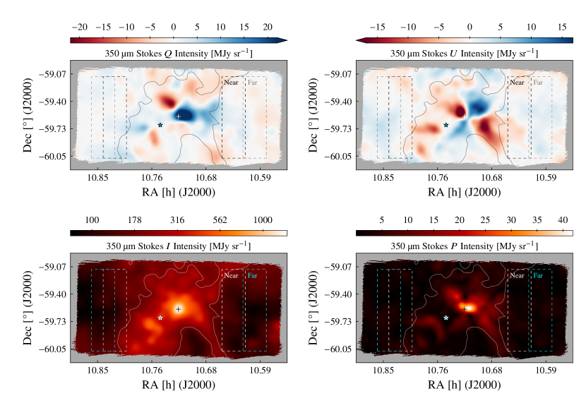
Figure 1.— BLASTPol 350 $\mathrm{\SIUnitSymbolMicro m}$ intensity maps of the Carina Nebula in Stokes $Q$ (top left), $U$ (top right), $I$ (bottom left), and $P$ (bottom right). The dashed rectangles show the Near (white or black) and Far (cyan or gray) reference regions. The data used in this analysis are enclosed by the solid contour, which is determined by a threshold cut on Stokes $I$ at 850 $\mathrm{\SIUnitSymbolMicro m}$ (see text). The crosshair shows the location of the peak in $I$, while the star-shaped marker shows the position of $\eta$ Car. Note that the $I$ map is displayed on a logarithmic scale, while the other maps are on a linear scale.

2.3. Calibration

The TOAST BLASTPol maps are initially produced in the same units as the TOD: raw ADC counts. They must be calibrated into physical units of MJy sr^-1. Calibration is achieved using a dust spectral energy distribution (SED) obtained from the Planck all-sky dust model described in Planck Collaboration XI (2014). This model is also discussed in more detail in Section 3.5. The model dust morphology is defined by the optical depth at a reference frequency. Using the model SED, the dust total intensity at this frequency is scaled to and integrated over top-hat approximations to each of the three BLASTPol bands. This procedure produces model maps for the dust Stokes $I_{\lambda}$ at $\lambda$ = 250, 350, and 500 $\mathrm{\SIUnitSymbolMicro m}$. These model maps are fitted to the actual BLASTPol maps in these three bands according to

$$I_{\lambda}(\mathrm{BLASTPol})=A_{\lambda}\left(I_{\lambda}(\mathrm{model})+B_{\lambda}\right).$$ (1)

The BLASTPol maps $Q_{\lambda}$ and $U_{\lambda}$ were calibrated using the above gain as well ($A_{\lambda}^{-1}$ in MJy sr^-1 count^-1). However, they also had to be divided by $\gamma_{\lambda}$, the measured instrumental polarization efficiencies in each waveband, which are reported in Galitzki et al. (2014a). While this procedure corrected the map slopes, the polarization maps also had arbitrary DC offsets $B_{\lambda}$ that could not be determined using Equation 1, because equivalent dust model maps $Q_{\lambda}(\mathrm{model})$ and $U_{\lambda}(\mathrm{model})$ do not exist. As discussed in the next section, polarization spectrum analysis normally proceeds by subtracting diffuse background emission from the maps before computing polarization quantities. However, a case with no background subtraction is presented here as well, for which the determination of the DC offsets is important. To determine the offsets, the Planck HFI 850 $\mathrm{\SIUnitSymbolMicro m}$ map of dust emission was color-corrected by scaling it to the dust model map in each of the BLASTPol bands:

$$I_{\lambda}(\mathrm{model})=a_{\lambda}\left(I_{850}(\mathrm{HFI})+b_{\lambda}\right).$$ (2)

In principle, the linearity of this scaling requires that the dust be isothermal at temperature $T_{d}$, and that it have an emissivity with consant power-law spectral index $\beta_{d}$ (Section 3.5). In practice, it was found that rejection of map pixels that were high-temperature outliers in the all-sky dust model was sufficient for good linearity. Model maps $Q_{\lambda}(\mathrm{model})$ and $U_{\lambda}(\mathrm{model})$ could then be obtained by color-correcting $Q_{850}$ and $U_{850}$ to the BLASTPol bands using scale factor $a_{\lambda}$. The DC offsets of the calibrated BLASTPol polarization maps were then obtained by plotting pixel values of $Q_{\lambda}(\mathrm{BLASTPol})$ versus $Q_{\lambda}(\mathrm{model})$, and likewise for $U_{\lambda}$.

2.4. Diffuse Emission Subtraction

Care must be taken to ensure that the polarized intensity observed at each sightline in this analysis is restricted to emission from the molecular cloud itself, and does not include a component from diffuse Galactic dust in the foreground or background. Contamination from diffuse Galactic emission could have a significant effect on the measured polarization, since diffuse emission has been shown, on average, to have a higher linear polarization fraction than emission from denser regions within molecular clouds (Planck Collaboration Int. XIX, 2015).

Typically, to correct for diffuse emission, a reference region adjacent to the cloud (but outside of it) is chosen. In each of $I$, $Q$, and $U$, the mean intensity within the reference region is assumed to be a level of diffuse emission from foreground or background dust that applies uniformly to the sightlines within the cloud as well. This intensity level is subtracted from its respective Stokes map before proceeding with the polarization analysis. For this analysis of Carina, two narrow vertical rectangular reference regions were chosen that bracket the cloud on its east and west sides. The intensity level subtracted was the mean intensity of all the pixels lying within the two rectangular regions. As shown in Figure 1, two different sets of two rectangles were selected, a closer pair called the “Near” reference region, and a pair farther out in RA, referred to as the “Far” reference region. All the analysis presented herein was repeated for both the Near and Far reference regions, in order to evaluate the dependence of the result on the choice of reference region. Furthermore, for the purpose of comparison, we present an additional analysis for which no diffuse emission subtraction is carried out.

A large-scale, roughly north-south systematic gradient exists in the BLASTPol Carina Nebula maps due to receiver $1/f$ noise. This gradient is corrected using Herschel SPIRE $I$ maps of the same region in the same bands (see Appendix A). However, choosing the reference regions to be elongated vertically, and averaging over them, mitigates the effects of any residual gradient still present after this correction.

In selecting reference regions that lie just outside (or well outside) the molecular cloud, the question arises of which map pixels are associated with the cloud in the first place. These pixels were chosen by applying a threshold cut on Stokes $I$ at 850 $\mathrm{\SIUnitSymbolMicro m}$ (the intensity in this waveband being used as a proxy for dust column density). The cloud is then defined as the region enclosed by the contour where $I_{850}=(3/2)\langle I_{850}\rangle_{\mathrm{Far}}$, with the angle brackets denoting the mean intensity over the Far reference region. This contour is overlaid on the maps in Figure 1; pixels outside of it were excluded from the polarization spectrum analysis. The ratio of 3/2 was chosen because it is comparable to the 850 $\mathrm{\SIUnitSymbolMicro m}$ intensity ratio between the Vela C cloud regions defined by Hill et al. (2011), and the reference regions used in the BLASTPol polarization spectrum analysis of Vela C (Gandilo et al., 2016). Data that lie outside vertical lines coinciding with the inner vertical edges of the reference region rectangles on either side of the map have also been excluded from the analysis in both the Near and Far cases. In the case with no background subtraction, the Far reference region rectangles are used for this purpose.

After carrying out the diffuse emission subtraction (if any) the Stokes parameter maps are spatially-downsampled by a factor of 15 using constant-value interpolation. This step increases the pixel size from $10^{\prime\prime}$ to $2^{\prime}.5$, roughly Nyquist-sampling the $4^{\prime}.8$ beam of the smoothed maps. The pixel covariance maps are downsampled in the same manner.

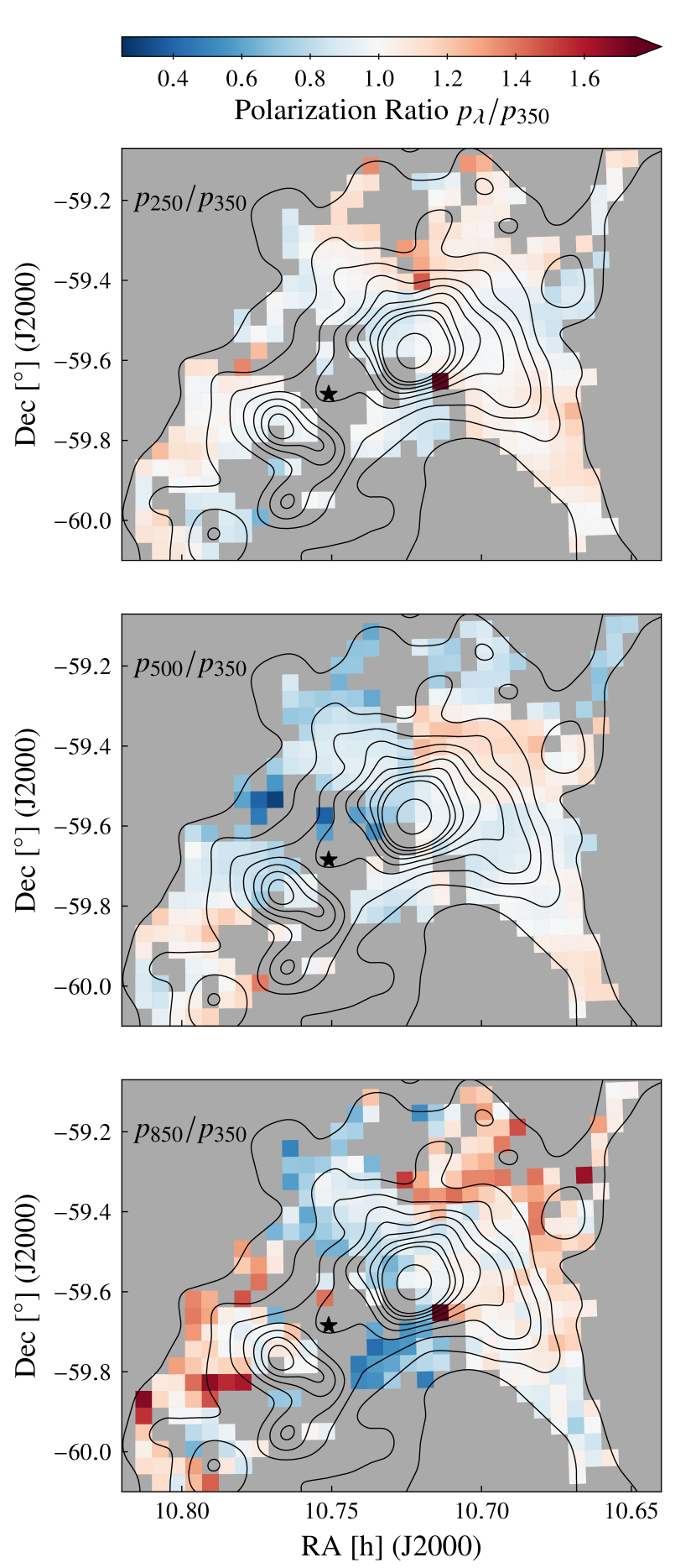
Figure 2.— Spatial maps of the polarization ratios $p_{250}/p_{350}$ (top), $p_{500}/p_{350}$ (middle), and $p_{850}/p_{350}$ (bottom). The contours show percentages of the 350 $\mathrm{\SIUnitSymbolMicro m}$ peak intensity ranging from 5% to 50% in 5% increments, along with a 75% contour. The black star-shaped marker shows the location of $\eta$ Car.

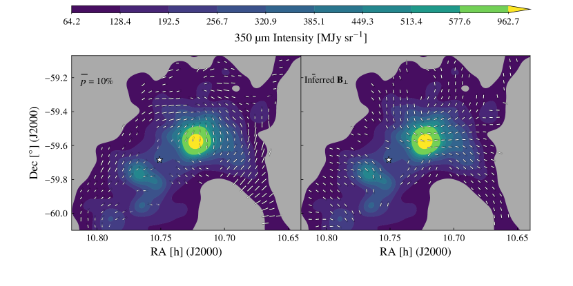
Figure 3.— Left panel: polarization pseudo-vectors showing the direction $\psi$ of the linearly-polarized radiation measured by BLASTPol at 350 $\mathrm{\SIUnitSymbolMicro m}$ in Carina, for those sightlines surviving the data cuts (see text). The lengths of the pseudo-vectors are scaled to show the fractional linear polarization $p$ for each sightline, as a percentage of the total intensity. The length scale is given by the key in the upper left. Right panel: pseudo-vectors showing the corresponding directions of the projected magnetic field $\mathbf{B}_{\perp}$ within the cloud. In this case, the pseudo-vectors are all the same length, in order to show the large-scale structure of the field more clearly. The color scale is for the filled contours in both panels, which show the 350 $\mathrm{\SIUnitSymbolMicro m}$ intensity $I$ in MJy sr^-1. The star-shaped markers indicate $\eta$ Car.

2.5. Polarimetry

The Stokes parameters are used to compute the net linear polarization of the dust emission

$$P=\sqrt{Q^{2}+U^{2}},$$ (3)

as well as the fractional linear polarization

$$p=\frac{P}{I}.$$ (4)

The angle $\psi$ defining the direction of the linear polarization on the sky is given by

$$\psi=\frac{1}{2}\arctan(U,Q).$$ (5)

where the two-argument form of the arctan function is used in order to evaluate the angle quadrant properly. The IAU polarization angle convention is used; for a polarization pseudo-vector viewed on the sky in Equatorial coordinates, $\psi$ increases counter-clockwise from $0$\mathrm{\SIUnitSymbolDegree}$$ in the the north-south direction, and ranges from $-90$\mathrm{\SIUnitSymbolDegree}$$ to $+90$\mathrm{\SIUnitSymbolDegree}$$.

The TOAST pixel covariances are used to compute the variances in these quantities, $\sigma_{p}^{2}$ and $\sigma_{\psi}^{2}$, using error propagation (see Appendix B). Since $P$ and $p$ are restricted to positive values, any noise in $Q$ and $U$ positively biases these quantities. The polarization fraction is de-biased approximately using a rudimentary method that is acceptable for high signal-to-noise in $p$ (Wardle & Kronberg, 1974; Montier et al., 2015):

$$p_{\mathrm{db}}=\sqrt{p^{2}-\sigma_{p}^{2}}.$$ (6)

All of the $p$ values used in the polarization spectrum analysis (Section 3) have been de-biased in this way. Note, however, that the map of $P$ shown in the lower right panel of Figure 1 is presented for visualization purposes only, and has not been de-biased.

Once maps of $p$ and $\psi$ have been produced, data cuts are applied that have been customary for submillimeter polarization spectrum analyses in the literature. The first is a signal-to-noise cut on map pixels using a threshold of $p_{\mathrm{db}}>3\sigma_{p}$. Only pixels for which this condition holds simultaneously in all four bands are kept. The second data cut is intended to mitigate the circumstance in which the different wavebands sample different cloud components along the line of sight, each with differing line-of-sight components of the magnetic field, and hence differing polarization fractions. This situation would lead to artificial variation with wavelength in the measured polarization spectrum for the sightline in question: variation which is not intrinsic to any particular physical location within the cloud. Under the assumption that a sightline having a plane-of-sky component of $\mathbf{B}$ that is constant with wavelength implies (at least in a statistical sense) a constant line-of-sight component of $\mathbf{B}$ as well, the condition is imposed that the difference $|\Delta\psi|<15$\mathrm{\SIUnitSymbolDegree}$$ between any two of the four wavebands. The stringent maximum angle difference of $10$\mathrm{\SIUnitSymbolDegree}$$ used in past analyses, including Gandilo et al. (2016), was relaxed for Carina, in order to include more sightlines in the analysis.

After the downsampling and data cuts, polarization data remained for 314, 285, and 270 sightlines respectively for the three cases of diffuse emission subtraction using the Far reference region, subtraction using the Near reference region, and no diffuse emission subtraction at all. Figure 2 shows maps of the polarization fraction ratios for those pixels surviving the data cuts in the Far reference region case. These are the ratios $p_{\lambda}/p_{350}$, for $\lambda\in\{250,500,850\}$ $\mathrm{\SIUnitSymbolMicro m}$. These discrete values sample the polarization spectrum over this wavelength range, and are analyzed in detail in the next section.

For all map pixels surviving the data cuts, the left panel of Figure 3 represents the linear polarization at 350 $\mathrm{\SIUnitSymbolMicro m}$ as pseudo-vectors of length $p$ and direction $\psi$. The pseudo-vectors are overlaid on filled contours showing the 350 $\mathrm{\SIUnitSymbolMicro m}$ intensity over the cloud. The “polarization-hole effect” is evident here, in which the polarization fraction is lower near bright intensity peaks. This effect has been noted in past submillimeter polarimetry observations (Matthews et al., 2001). The right panel of Figure 3 shows the corresponding inferred directions (but not magnitudes) of the plane-of-sky component of the magnetic field, $\mathbf{B}_{\perp}$. These directions are rotated by $90$\mathrm{\SIUnitSymbolDegree}$$ relative to the $\mathbf{E}$-field polarization direction of the radiation.

3. Results

3.1. Median Polarization Ratios

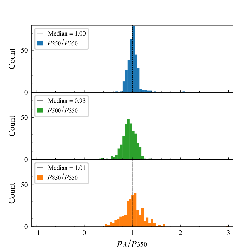
Figure 4.— Histograms of the polarization ratios $p_{\lambda}/p_{350}$ for diffuse emission subtraction using the Far reference region. The dashed vertical lines show the median of each distribution.

Figure 4 shows histograms of the polarization ratios $p_{\lambda}/p_{350}$, specifically the distributions of these ratios over the cloud for the case of diffuse emission subtraction using the Far reference region. For consistency with Gandilo et al. (2016), the widths of the distributions were quantified using the median absolute deviation (MAD), defined as

$$\mathrm{MAD}\equiv\mathrm{median}\left(|x_{i}-\mathrm{median}(x_{i})|\right),$$ (7)

where the quantities $x_{i}$ are the measurements in question. Table 1 lists the median ratios and MADs for all three types of diffuse emission subtraction. Although the two cases with background subtraction show a slight minimum at 500 $\mathrm{\SIUnitSymbolMicro m}$, none of the results are significantly different from a flat spectrum, with a polarization ratio of unity to within 15% in each band. This result is independent of the method of diffuse emission subtraction: a very similar outcome to that of Gandilo et al. (2016).

Table 1Medians and MADs of Polarization Ratios ($p_{\lambda}/p_{350}$).

Diffuse Emission	$250~{}$\mathrm{\SIUnitSymbolMicro m}$$	$500~{}$\mathrm{\SIUnitSymbolMicro m}$$	$850~{}$\mathrm{\SIUnitSymbolMicro m}$$
Subtraction Method
Far	$1.00\pm 0.06$	$0.93\pm 0.10$	$1.01\pm 0.12$
Near	$1.02\pm 0.06$	$0.93\pm 0.08$	$0.99\pm 0.12$
None	$1.14\pm 0.08$	$0.96\pm 0.08$	$0.95\pm 0.12$

3.2. Polarization Ratios from Scatter Plots of $p_{\lambda}$ vs. $p_{350}$

An alternative method for determining the polarization ratios, averaged over the cloud, is to produce linear fits to scatter plots of $p_{\lambda}$ versus $p_{350}$. The polarization spectrum then consists of the best-fit linear slopes as a function of wavelength. For this fitting procedure, the least absolute deviation was used to optimize the fit parameters. This method is more robust to outliers than least-squares fitting. For each fit, an uncertainty on the slope was estimated using bootstrap resampling (Press et al., 1992, p. 691). The fit was repeated for each of 10,000 random selections of the data points (with replacement), and the uncertainty was taken to be the standard deviation of this ensemble of fit parameter values. The linear fits are shown in Figure 5 for the case of diffuse emission subtraction using the Far reference region.

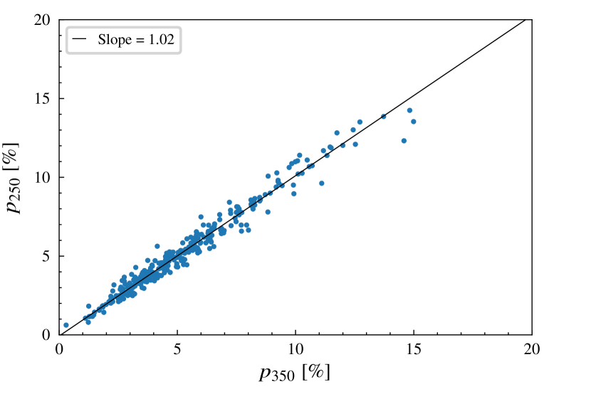
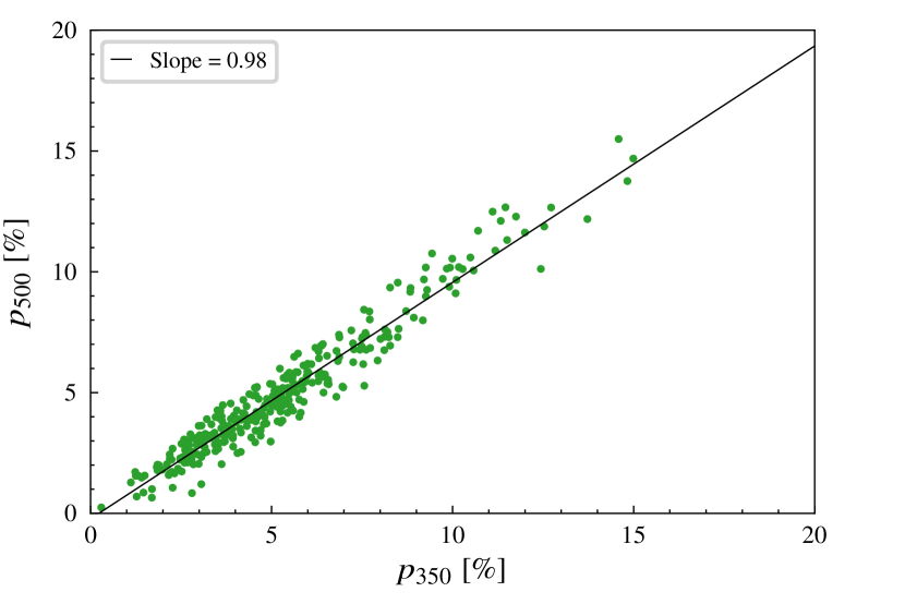
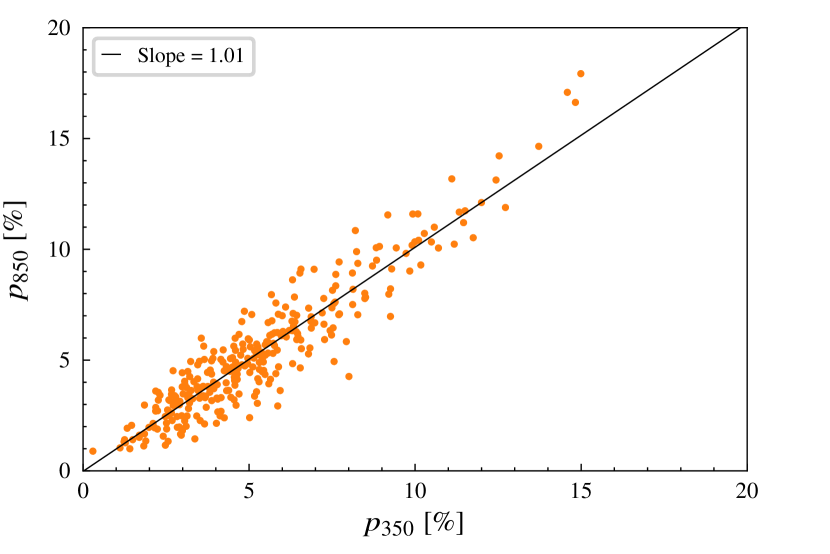
Figure 5.— Linear fits to scatter plots of $p_{\lambda}$ versus $p_{350}$ for $\lambda$ = 250 $\mathrm{\SIUnitSymbolMicro m}$ (top), $\lambda$ = 500 $\mathrm{\SIUnitSymbolMicro m}$ (middle), and $\lambda$ = 850 $\mathrm{\SIUnitSymbolMicro m}$ (bottom). These plots are shown for diffuse emission subtraction using the Far reference region.

Table 2 lists the slopes of the linear fits to each waveband, along with their uncertainties, for the cases of background subtraction using the Far reference region, using the Near reference region, and for the case of no background subtraction. For the Near and Far cases, the feature of a very slight minimum at 500 $\mathrm{\SIUnitSymbolMicro m}$ occurs using this method, just as it did for the median ratios. The polarization spectra obtained using the linear fitting are once again flat to within $\pm$15%.

Table 2Slopes of Linear Fits to $p_{\lambda}$ versus $p_{350}$.

Diffuse Emission	$250~{}$\mathrm{\SIUnitSymbolMicro m}$$	$500~{}$\mathrm{\SIUnitSymbolMicro m}$$	$850~{}$\mathrm{\SIUnitSymbolMicro m}$$
Subtraction Method
Far	$1.02\pm 0.01$	$0.98\pm 0.02$	$1.01\pm 0.02$
Near	$1.05\pm 0.01$	$0.95\pm 0.02$	$1.03\pm 0.03$
None	$1.14\pm 0.02$	$1.02\pm 0.02$	$0.90\pm 0.04$

3.3. Fits to $p(\lambda)$

Two different functional forms for $p(\lambda)$ were fitted to the per-pixel $p$ measurements across the bands: a power law

$$p(\lambda)=a_{1}\left(\frac{\lambda}{\lambda_{0}}\right)^{b_{1}},$$ (8)

and a second-order polynomial

$$p(\lambda)=a_{2}\left[b_{2}\left(\lambda-\lambda_{0}\right)^{2}+c_{2}\left(\lambda-\lambda_{0}\right)+1\right].$$ (9)

Here, $\lambda_{0}$ = 350 $\mathrm{\SIUnitSymbolMicro m}$, and for both models, $a$ is an overall normalization constant (it is the fitted value of $p_{350}$). The models are intended to probe the shape of the per-pixel polarization spectra over the wavelength range of 250 $\mathrm{\SIUnitSymbolMicro m}$ to 850 $\mathrm{\SIUnitSymbolMicro m}$. The power-law model investigates whether the spectra are increasing or decreasing. The quadratic model, in addition, allows for the polarization spectra to have minima or maxima somewhere within this wavelength range.

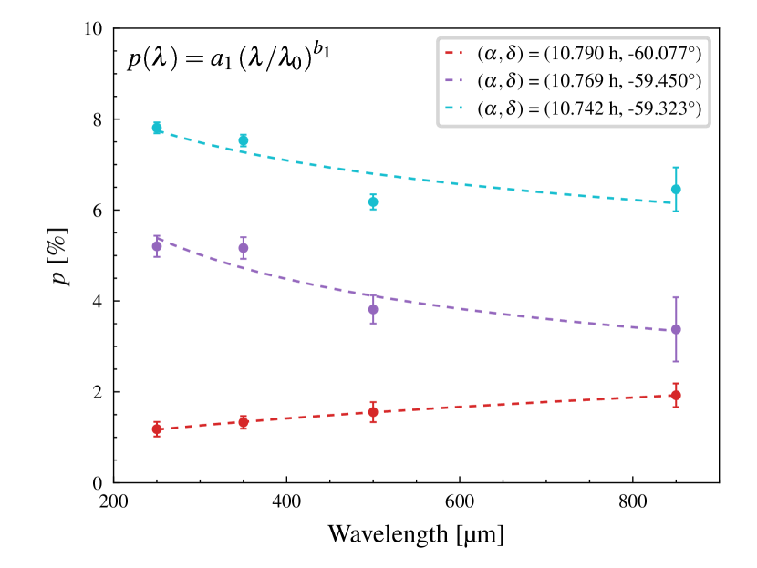
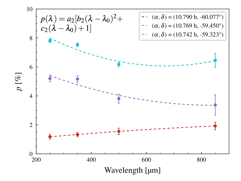
Figure 6.— Power-law (top) and quadratic (bottom) fits to $p(\lambda)$ for three example pixels. The plots are shown for diffuse emission subtraction using the Far reference region.

Table 3Medians and MADs of $p(\lambda)$ Fit Parameters

Diffuse Emission	Power Law Fit		Polynomial Fit
Subtraction Method	$b_{1}$	$p_{350}/a_{1}$	$b_{2}$ ($\times 10^{-6}$)	$c_{2}$ ($\times 10^{-4}$)	$p_{350}/a_{2}$
Far	$-0.01\pm 0.10$	$1.01\pm 0.03$	$0.8\pm 1.3$	$-3.1\pm 4.9$	$1.03\pm 0.03$
Near	$-0.04\pm 0.10$	$1.01\pm 0.03$	$0.9\pm 1.4$	$-4.2\pm 4.6$	$1.03\pm 0.03$
None	$-0.14\pm 0.10$	$0.96\pm 0.04$	$1.1\pm 1.1$	$-8.0\pm 4.6$	$0.96\pm 0.03$

Figure 6 shows the results of the power-law and quadratic fitting for three example pixels. In these plots, the error bars in each band are derived from the TOAST covariances (Appendix B). After fitting to the per-pixel spectra, the distributions of the fit parameters were analyzed. The medians and MADs are listed in Table 3 for the fit parameters relevant to the spectral shape, i.e. $b_{1}$, $b_{2}$, and $c_{2}$. This table also lists the median $\pm$ MAD values of the ratios $p_{350}/a$, which indicate the extent to which the model value for the fractional polarization at 350 $\mathrm{\SIUnitSymbolMicro m}$ matches the measured value. The distributions of the spectral-shape fit parameters for the Far reference region case are shown in Figure 7 for the power-law fit, and in Figure 8 for the quadratic fit.

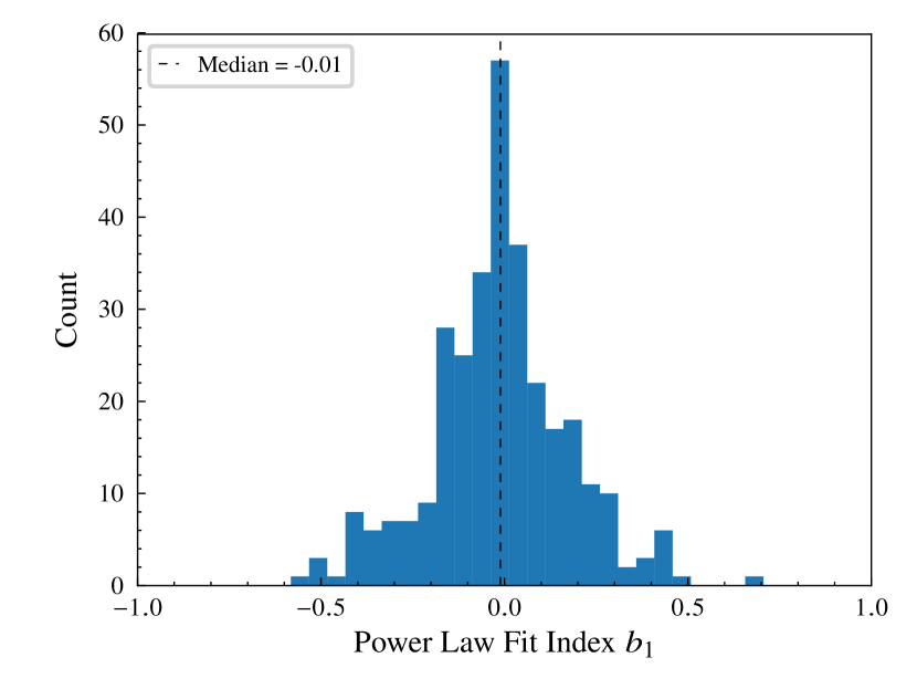
Figure 7.— Histogram of the power-law fit parameter $b_{1}$ from Equation 8.

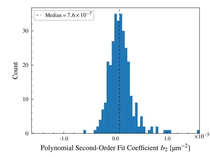
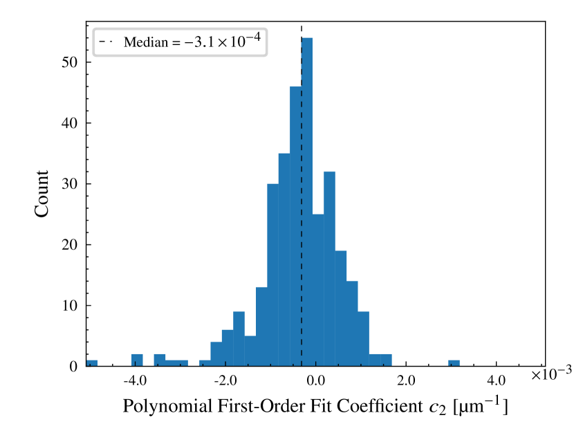
Figure 8.— Histograms of the polynomial fit parameters $b_{2}$ (top) and $c_{2}$ (bottom) from Equation 9.

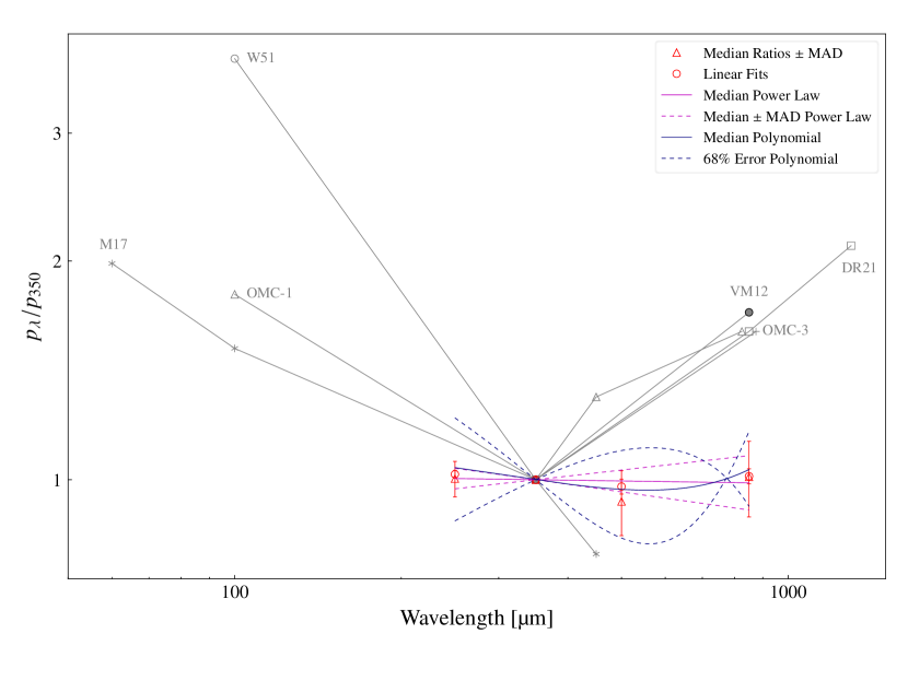
Figure 9.— Polarization spectra from previous work in gray, with new BLASTPol/Planck Carina data added in color. The gray data points at 850 $\mathrm{\SIUnitSymbolMicro m}$ have been offset horizontally to distinguish them. The W51 and OMC-1 $p_{100}/p_{350}$ values and the DR21 $p_{1300}/p_{350}$ values are from Vaillancourt (2002). All previous measurements at 850 $\mathrm{\SIUnitSymbolMicro m}$ are from Vaillancourt & Matthews (2012). The solid circle (VM12) is the median of these 850 $\mathrm{\SIUnitSymbolMicro m}$ measurements over 15 clouds. The OMC-1 $p_{450}/p_{350}$ value is from Vaillancourt et al. (2008). The M17 points are from Zeng et al. (2013). The red triangles show the median polarization ratios with MAD error bars. The red circles are the best-fit slopes of linear fits to scatter plots of $p_{\lambda}$ versus $p_{350}$. The magenta lines show spectra produced using the power-law fit parameters, while the dark blue lines show spectra produced using the quadratic fit parameters. For these two cases, the solid lines are spectra produced using the median fit parameters, while the dashed lines reflect the distribution in the fit parameters (see text).

3.4. Summary of Polarization Spectrum Measurements

The result of a flat spectrum for Carina computed using all the previously-described methods is shown in Figure 9 for the case of diffuse emission subtraction using the Far reference region. The median polarization ratios $\pm$ MADs (Section 3.1) are shown as red triangles. The polarization ratios from linear fits to scatter plots of $p_{\lambda}$ versus $p_{350}$ are shown as red circles, with error bars based on bootstrap resampling (Section 3.2). Representative power-law and quadratic fits to per-pixel polarization spectra (Section 3.3) are also shown. For the power-law fit, the mean and dispersion among the per-pixel polarization spectra are demonstrated by plotting the power-law model corresponding to $\mathrm{median}(b_{1})$ as a solid magenta line, and plotting the models corresponding to $\mathrm{median}(b_{1})\pm\mathrm{MAD}(b_{1})$ as dashed magenta lines. Similarly, for the second-order polynomial fit, the parabola corresponding to the median values of $b_{2}$ and $c_{2}$ is plotted as a solid dark blue line. However, the fit parameters $b_{2}$ and $c_{2}$ are highly anti-correlated, with Pearson correlation coefficient $\rho_{c_{2},b_{2}}=-0.92$ for the Far reference region case. Therefore, it was not sufficient to simply plot extremal models using the median $\pm$ MAD values of each fit parameter individually. The 68% error ellipse of their joint distribution was constructed by diagonalizing the covariance matrix of $b_{2}$ and $c_{2}$ using eigenvalue decomposition. The major axis of the resulting ellipse had endpoints at $(c_{2},b_{2})=(-1.8\times 10^{-3},4.2\times 10^{-6})$ and at $(c_{2},b_{2})=(9.9\times 10^{-4},-2.3\times 10^{-6})$. The dashed dark blue lines in Figure 9 correspond to the parabolas having these extremal fit parameter values.

3.5. Effect of Environment

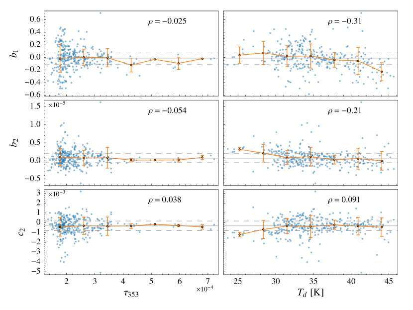
Figure 10.— Plots of polarization spectrum shape parameters versus dust optical depth $\tau_{353}$ (left column) or versus dust temperature $T_{d}$ (right column) for the case of diffuse emission subtraction using the Far reference region. From top row to bottom, the parameters are, respectively, the spectral index $b_{1}$ of the power-law fit, the second-order coefficient $b_{2}$ of the quadratic fit, and the first-order coefficient $c_{2}$ of the quadratic fit. The light blue points show the data for every sightline, while the orange points and error bars show the mean and standard deviation of each shape parameter within bins linearly-spaced in $\tau_{353}$ or $T_{d}$. The horizontal gray lines show the median (solid) and median $\pm$ MAD (dashed) parameter values over the whole cloud.

An investigation was undertaken to probe whether the shape of the polarization spectrum over these four bands exhibits any dependence on the molecular cloud environment. Polarization spectrum parameters were correlated with two environmental parameters: dust temperature $T_{d}$, and dust optical depth at 353 GHz $\tau_{353}$. The latter is proportional to the dust column density. These parameters were obtained from the Planck all-sky dust model (Planck Collaboration XI, 2014) first mentioned in Section 2.3. This model is generated by fitting a modified blackbody SED to the high-frequency dust $I$ maps from HFI at 353, 545, and 857 GHz, along with a highest-frequency map from IRAS 100 $\mathrm{\SIUnitSymbolMicro m}$ data. This SED is of the form

$$I_{\nu}(\nu)=\tau_{\nu_{0}}\left(\frac{\nu}{\nu_{0}}\right)^{\beta_{d}}B_{\nu}(\nu,T_{d}).$$ (10)

In Equation 10, $\beta_{d}$ is the power-law spectral index of the frequency-dependent dust emissivity, $B_{\nu}$ is the Planck function, and $T_{d}$ is the dust temperature. The parameter $\tau_{\nu_{0}}$ is the dust optical depth at a reference frequency of $\nu_{0}=353~{}$\mathrm{GHz}$$. In Planck Collaboration XI (2014), it is emphasized that these three parameters are only approximations to the true dust properties. A single-component model has been assumed, whereas in reality multiple temperature components could exist along any given line of sight. Therefore the model parameters $\tau_{353}$ and $T_{d}$ are used here only to establish the relative ordering among sightlines in order to search for very obvious trends, which, if present, would lend themselves to a more detailed future investigation. Gandilo et al. (2016) used a similar dust SED model fitted to the Herschel-SPIRE 160, 250, 350, and 500 $\mathrm{\SIUnitSymbolMicro m}$ maps of Vela C. This fit assumed $\beta_{d}=2$ and obtained values for $T_{d}$ and column density $N_{H}$. The per-pixel polarization spectrum shape parameters $b_{1}$, $b_{2}$, and $c_{2}$ defined in Section 3.3 were plotted against $T_{d}$ and $N_{H}$ in order to search for a dependence of spectral shape on environment. For the Carina Nebula however, due to the limited spatial extent of the available Herschel maps, it was not possible to carry out such a fit using the exact same reference region for diffuse emission subtraction as was used for the BLASTPol maps. Thus, we opted to use the Planck all-sky dust model instead. Using the Planck-derived $\tau_{353}$ as the environmental density parameter rather than computing $N_{H}$ also avoids making assumptions about the dust opacity, $\sigma_{353}=\tau_{353}/N_{H}$, within our region.

Figure 10 shows the results of plotting the power-law and polynomial fit parameters versus temperature and optical depth. In addition to the points for every individual sightline, the fit parameters are binned into seven evenly-spaced bins in $T_{d}$ or $\tau_{353}$. The binned curves appear quite flat. For the most part, the mean values of the fit parameters within each bin (orange points) lie well within the median $\pm$ MAD range of the fit parameters over the whole cloud (bounded by the gray dashed lines). Exceptions to this are the first $T_{d}$ bin for $c_{2}$ and $b_{2}$, and the last $T_{d}$ bin for $b_{1}$. However, these bins only contain a handful of points each. Each panel of Figure 10 also shows the value of the Pearson correlation coefficient $\rho$ for the scatter plot in question. Overall, strong evidence for trends in polarization spectrum shape with environment are not observed.

4. Discussion

As shown in Figure 9, the result of a polarization spectrum that is flat to within $\pm$15% is inconsistent with the results of measurements of a number of molecular clouds obtained by ground-based submillimeter telescopes. Recall (Section 1) that the BLASTPol/Planck submillimeter polarization spectrum for the Vela C GMC presented by Gandilo et al. (2016) was also much flatter than the ground-based spectra. As a potential explanation for this discrepancy, Gandilo et al. (2016) posited that ground-based observations were limited to the densest sightlines within molecular clouds, in a very different regime of column density compared to the cloud-averaged case for BLASTPol. This can be quantified using the Planck 850 $\mathrm{\SIUnitSymbolMicro m}$ intensity as a proxy for column density. Although this proxy (unlike $\tau$) is not completely free from dependence on dust temperature, it was the only method available for comparing column density between the BLASTPol and ground-based measurements. Table 4 below shows a comparison of the median and interquartile range of the 850 $\mathrm{\SIUnitSymbolMicro m}$ intensity computed for Carina (this work), for Vela C (Gandilo et al., 2016), for a translucent molecular cloud (Ashton et al., 2018), and for ground-based measurements of 17 molecular clouds, which were calculated by Gandilo et al. (2016) using online data provided by Vaillancourt & Matthews (2012).

Table 4Comparison of quartiles in 850 $\mathrm{\SIUnitSymbolMicro m}$ intensity in MJy sr^-1 between Planck measurements and ground-based measurements of molecular clouds. The Carina Nebula values are computed over the sightlines passing the data cuts for the case of diffuse emission subtraction using the Far reference region.

	$1^{\mathrm{st}}$ Quartile	Median	$3^{\mathrm{rd}}$ Quartile
Translucent Cloud (Ashton et al., 2018)	3.1	3.4	4.1
Vela C (Gandilo et al., 2016)	6.5	9.1	14.1
Carina Nebula (this work)	7.6	10.8	17.6
Ground-based, 17 molecular clouds (Vaillancourt & Matthews, 2012)	300	637	1327

The comparison shows that the median 850 $\mathrm{\SIUnitSymbolMicro m}$ intensity for the Carina Nebula is quite similar to that of the Vela C measurement, indicating a broadly similar regime in column density. In comparison, the median intensity of the ground-based measurements is nearly two orders of magnitude higher.

Another interesting comparison is to the analysis of the most recent Planck data release (PR3) in  Planck Collaboration XI (2018). The equivalent information to the polarization spectrum is reported by Planck in terms of the difference in power law spectral indicies of the SEDs for total intensity and for polarization, $\beta_{d}^{I}$ and $\beta_{d}^{P}$. Under the simplistic assumption that the dust grains contributing to polarized and to overall emission are all isothermal at temperature $T_{d}$, these two SEDs can be written as $I(\nu)\propto\left(\nu/\nu_{0}\right)^{\beta_{d}^{I}}B_{\nu}(\nu,T_{d})$ and $P(\nu)\propto\left(\nu/\nu_{0}\right)^{\beta_{d}^{P}}B_{\nu}(\nu,T_{d})$. It can then be shown that the quantity computed in this work, the polarization ratio, is given by

$$\frac{p(\nu)}{p(\nu_{0})}=\left(\frac{\nu}{\nu_{0}}\right)^{\beta_{d}^{P}-\beta_{d}^{I}}.$$ (11)

Therefore, a measurement of $\beta_{d}^{P}<\beta_{d}^{I}$ would imply a polarization spectrum that was falling with frequency, or rising with wavelength. In the analysis of the PR3 maps, polarized emission was investigated for six nested sky patches at high Galactic latitude. A model was fitted to the angular cross power spectra between Planck frequency maps. This model included a power-law dependence on multipole moment ($\ell$), a power-law frequency dependence for polarized synchrotron emission, and a modified blackbody SED with power-law emissivity for polarized dust emission at an assumed dust temperature $T_{d}=19.6~{}$\mathrm{K}$$. The result, averaged over all sky patches and multipole bins, was $\beta_{d}^{P}=1.53\pm 0.02$. No statistically-significant difference from the spectral index for total intensity was found: $\beta_{d}^{P}-\beta_{d}^{I}=0.05\pm 0.03$ (Planck Collaboration XI, 2018). This result implies a flat polarization spectrum, on average, at millimeter wavelengths.

In addition to this overall agreement with the high-latitude diffuse emission, there is now striking agreement among BLASTPol molecular cloud targets in the Galactic plane. The result of a flat spectrum in polarization fraction has now been reproduced for measurements of a cold, dense molecular cloud (Gandilo et al., 2016), a translucent molecular cloud (Ashton et al., 2018) and a more evolved, warmer molecular cloud being actively-heated by many internal stellar sources (this work). A direct comparison of these three results is shown in Figure 11. Some care should be taken in the interpretation of this figure, since the polarization spectrum from Ashton et al. (2018) is normalized to the 850 $\mathrm{\SIUnitSymbolMicro m}$ band, whereas the other two polarization spectra are normalized to 350 $\mathrm{\SIUnitSymbolMicro m}$. Even so, despite the differing radiative environments and densities of these targets, the result of a flat submillimeter polarization spectrum persists as a common property of these molecular clouds.

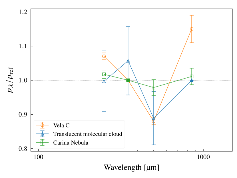
Figure 11.— Examples of three polarization spectra from the BLASTPol 2012 flight. Shown are measurements of a translucent molecular cloud near to Vela C on the sky (Ashton et al., 2018, triangular points), measurements of the Vela C molecular cloud (Gandilo et al., 2016, circular points), and measurements of the Carina Nebula (this work, square points). For Vela C and Carina, the points shown, and the associated error bars, are from linear fits to scatter plots of $p_{\lambda}$ versus $p_{\mathrm{ref}}$, with a reference band of 350 $\mathrm{\SIUnitSymbolMicro m}$. For the translucent cloud, the points shown, and the associated statistical error bars, come from linear fits to $Q_{\lambda}$ and $U_{\lambda}$ measured in the BLASTPol bands versus $Q_{\lambda}$ and $U_{\lambda}$ extrapolated to those bands (from a reference band of 850 $\mathrm{\SIUnitSymbolMicro m}$) using the Planck all-sky dust model. The filled points show which band is the reference band for each polarization spectrum plotted.

This result of a lack of significant wavelength-variation in the polarization spectrum for a cloud such as the Carina GMC, with significant internal heating from embedded sources, potentially has implications for theoretical grain alignment mechanisms. For example, the RAT mechanism (Section 1) predicts a higher grain alignment efficiency for dust grains that are less shielded from stellar radiation (Andersson et al., 2015). However, a detailed investigation of the implications of our result to grain-alignment theory is beyond the scope of this work. For the purpose of a baseline comparison to theory, we examine the model of a cold, dense molecular cloud with no internal sources presented in Bethell et al. (2007). Figure 12 shows this model over the wavelength range of interest. Overlaid are the previous ground-based polarization spectrum measurements first shown in Figure 9. In order to match the analysis method of Bethell et al. (2007), the BLASTPol/Planck data for Carina, and from Vela C from Gandilo et al. (2016), are shown here as the “total polarized fraction”, which is computed as $\left.\left(\sum_{j}P_{j}\right)\middle/\left(\sum_{j}I_{j}\right)\right.$, where $j$ indexes the pixels passing the data cuts. The results for these two BLASTPol targets are broadly consistent with the Bethell model, certainly showing a much closer correspondence than than the previous ground-based studies.

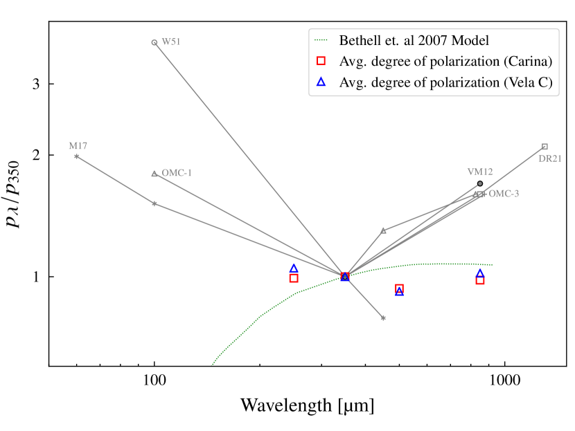
Figure 12.— Comparison with the polarization spectrum predicted by Bethell et al. (2007), shown as a green dotted line. The red squares represent the total polarized fraction of the Carina data (see text) normalized to 350 $\mathrm{\SIUnitSymbolMicro m}$, while the blue triangles show the same quantity for Vela C, as reported in Gandilo et al. (2016).

The negative slope of the ground-based polarization spectra in the far-infrared has been explained heuristically in terms of a very strong ETAC effect (Section 1), perhaps due to internal sources, in which hotter, less-shielded dust grains are preferentially more aligned, leading to a higher polarization fraction for the dust emission at shorter wavelengths (Hildebrand et al., 1999; Zeng et al., 2013). The righthand side of the V is more problematic, however: slopes of this steepness are not reproduced in the BLASTPol data. Furthermore, no theoretical models have been constructed that can reproduce the very large polarization ratios that are seen, in general, in the ground-based spectra. Regardless, we can conclude that the cloud-averaged submillimeter polarization spectra of two very different molecular clouds agree with the flat Bethell et al. (2007) prediction for externally-illuminated, dense molecular clouds with no internal radiation sources. Thus, it appears, at least from the BLASTPol measurements, that the internal sources do not significantly affect the cloud-averaged submillimeter polarization spectrum.

In light of the discrepancy between BLASTPol and ground-based submillimeter polarization spectrum results, a logical step for future work would be to repeat the measurements of the specific ground-based targets using more advanced ground-based polarimeters of higher sensitivity and mapping speed that are slated to come online in the near future. One example is the TolTEC camera (Bryan et al., 2018), which will probe wavelengths of 1 mm and longer. Another interesting avenue for future research is a more detailed investigation of the spatial variation of the polarization spectrum from point to point within a cloud, and the correlation of the spectral shape with environment. The BLASTPol data show some evidence of spatial variation (Figure 2), but no strong trends with environment. Ultimately this investigation is limited by the angular resolution of the data. The BLAST-TNG experiment (Galitzki et al., 2014b), which is currently scheduled for an Antarctic balloon flight in the Austral summer of 2018-2019, will greatly aid this effort. This polarimeter offers an order of magnitude more detectors than BLASTPol and will observe in the same bands with a much higher angular resolution of 31^′′ to 59^′′ FWHM. The combination of high resolution and full cloud-scale coverage offered by this experiment may also help test the hypothesis stated above that the discrepancy between the BLASTPol/Planck and ground-based measurements is due to the fact that the latter were only sensitive to the densest clumps within GMCs.

5. Summary

Measurements of the linear polarization along 314 sightlines were made by BLASTPol in the Carina Nebula in the 250, 350, and 500 $\mathrm{\SIUnitSymbolMicro m}$ wavebands. These data were combined with Planck 353 GHz (850 $\mathrm{\SIUnitSymbolMicro m}$) data from the same region in order to produce submillimeter polarization spectra. These spectra were calculated using several methods, including the median polarization ratios, slopes from linear fits to scatter plots of $p_{\lambda}$ versus $p_{350}$, and by fitting quadratic and power-law models $p(\lambda)$ to the per-pixel polarization spectra. No strong evidence was found for variation of the fitted parameters of these models as a function of cloud environment, as quantified by the dust temperature $T_{d}$ and dust optical depth $\tau_{353}$, which were obtained from the Planck all-sky dust model. The cloud-averaged polarization spectrum of the Carina Nebula appears flat to within $\pm$15% in the polarization ratio quantity $p_{\lambda}/p_{350}$, where $p_{\lambda}$ is the fractional linear polarization in a given waveband. This is at odds with previous ground-based measurements of the polarization spectrum of other molecular clouds, which showed a V-shaped spectrum, with a negative slope in the far-infrared, a positive slope towards millimeter wavelengths, and a pronounced minimum near 350 $\mathrm{\SIUnitSymbolMicro m}$. The flatness of the polarization spectrum in Carina is, however, in remarkably close agreement with BLASTPol/Planck measurements in other molecular clouds, including the measurement of the Vela C GMC (Gandilo et al., 2016), and of a translucent molecular cloud near to Vela C on the sky (Ashton et al., 2018). The shapes of the Vela C and Carina polarization spectra are both in relatively good agreement with the Bethell et al. (2007) theoretical prediction for an externally-illuminated, dense molecular cloud with no internal radiation sources.

Appendix A Correction of a Large-Scale Systematic Using Herschel Intensity Maps

During the initial polarization spectrum analysis of Carina, anomalously-high values were found for the polarization ratio $p_{850}/p_{350}$ for sightlines in the northern part of the cloud. The problem was determined to be in the BLASTPol data: receiver 1/$f$ noise led to the BLASTPol $I$ maps having a large-scale gradient in the north-south direction, which is perpendicular to the predominant scan direction during Carina observations. Systematically-high values of $I_{250}$, $I_{350}$, and $I_{500}$ led to systematically-low values of $p_{250}$, $p_{350}$, and $p_{500}$ in the north of the cloud. This bias in turn inflated the Planck-to-BLASTPol polarization ratio. Since the striping is predominantly in $I$, it could be corrected by differencing calibrated BLASTPol maps with publicly-available Herschel-SPIRE maps taken of Carina in the same bands.

The Herschel maps were first re-gridded to match the BLASTPol pixelization. A least-squares fit of a fifth-order polynomial was applied to the (BLASTPol $-$ Herschel) intensity values (for pixels within the left Far reference region rectangle) as a function of pixel $y$-coordinate. The fitted intensity as a function of map $y$-coordinate was extended horizontally across the entire map, to produce a model for the vertical gradient. This model was then subtracted from the BLASTPol $I$ maps in each band.

Only pixels within the left Far reference region rectangle were used in the fit, because there was a slight beam mismatch between the smoothed BLASTPol and smoothed Herschel intensity maps, leading to leakage of cloud structure (including intensity peaks) into the (BLASTPol $-$ Herschel) difference map. The left Far reference region rectangle happens to be free of such structure, meaning that most of the flux variation within it is due to the gradient alone. As the analysis progressed, more refined data cuts excluded some of the more extreme northern sightlines from the final data set. As a result, repeating the analysis of this paper with diffuse emission subtraction using the Far refrence region, and without the Herschel correction, results in relatively small changes to the median ratios of $\Delta\left(p_{\lambda}/p_{350}\right)$ = $-$0.007, +0.019, and $-$0.048 at 250, 500, and 850 $\mathrm{\SIUnitSymbolMicro m}$, respectively. Since the systematic does not change the final result of a polarization spectrum that is flat to within $\pm 15\%$ over all four bands, it was not deemed to be necessary to repeat the Herschel correction more carefully using maps of matching resolution.

Appendix B Error Propagation

The per-pixel variances of the polarization quantities, $P$, $p$, and $\psi$ are computed from the per-pixel covariance matrix of the Stokes parameters on the sky (as estimated by the TOAST map maker) using the following procedure. Each of the above three quantities can be expressed as a function $f(I,Q,U)$. If this function is approximated by its first-order Taylor series expansion about the mean of the pixel Stokes parameter values, then the variance in $f$ is given by:

$$\sigma^{2}_{f}=\left[\begin{array}[]{ccc}\frac{\partial f}{\partial I}&\frac{\partial f}{\partial Q}&\frac{\partial f}{\partial U}\end{array}\right]\left[\begin{array}[]{ccc}\sigma_{I}^{2}&\sigma_{IQ}&\sigma_{IU}\\ \sigma_{IQ}&\sigma_{Q}^{2}&\sigma_{QU}\\ \sigma_{IU}&\sigma_{QU}&\sigma_{U}^{2}\end{array}\right]\left[\begin{array}[]{c}\frac{\partial f}{\partial I}\\ \frac{\partial f}{\partial Q}\\ \frac{\partial f}{\partial U}\end{array}\right].$$ (B1)

Applying Equation B1 to each of Equations 3, 4, and 5 above yields the following results for the variances of the polarization quantities:

$$\sigma_{P}^{2}=\frac{1}{P^{2}}\left[\left(Q^{2}\right)\sigma_{Q}^{2}+\left(U^{2}\right)\sigma_{U}^{2}+\left(2QU\right)\sigma_{QU}\right],$$ (B2)

and

$$\sigma_{\psi}^{2}=\left(\frac{180$\mathrm{\SIUnitSymbolDegree}$}{\pi}\right)^{2}\frac{1}{4P^{4}}\left[\left(U^{2}\right)\sigma_{Q}^{2}+\left(Q^{2}\right)\sigma_{U}^{2}-\left(2QU\right)\sigma_{QU}\right].$$ (B3)

For notational convenience, we can define normalized Stokes parameters for linear polarization, given by $q\equiv Q/I$ and $u\equiv U/I$. Applying Equation B1 to these, we have

$$\sigma_{q}^{2}=q^{2}\left(\frac{\sigma_{I}^{2}}{I^{2}}+\frac{\sigma_{Q}^{2}}{Q^{2}}-2\frac{\sigma_{IQ}}{IQ}\right),$$ (B4)

$$\sigma_{u}^{2}=u^{2}\left(\frac{\sigma_{I}^{2}}{I^{2}}+\frac{\sigma_{U}^{2}}{U^{2}}-2\frac{\sigma_{IU}}{IU}\right),$$ (B5)

and

$$\sigma_{qu}=qu\left(\frac{\sigma_{I}^{2}}{I^{2}}+\frac{\sigma_{QU}}{{QU}}-\frac{\sigma_{IQ}}{IQ}-\frac{\sigma_{IU}}{IU}\right).$$ (B6)

The variance in $p$ can therefore be expressed compactly as

$$\sigma_{p}^{2}=\frac{1}{p^{2}}\left[\left(q^{2}\right)\sigma_{q}^{2}+\left(u^{2}\right)\sigma_{u}^{2}+\left(2qu\right)\sigma_{qu}\right].$$ (B7)

References

- Allen & Hillier (1993) Allen, D. A. & Hiller, D. J. 1993, Proceedings of the Astronomical Society of Australia, 10, 338
- Andersson et al. (2015) Andersson, B.-G., Lazarian, A. & Vaillancourt, J. E. 2015, ARA&A, 53, 501
- Ashton et al. (2018) Ashton, P. C., Ade, P. A. R., Angilè, F. E., et al. 2018, ApJ, 857, 10
- Bethell et al. (2007) Bethell, T. J., Chepurnov, A., Lazarian, A., et al. 2007, ApJ, 663, 1055
- Bryan et al. (2018) Bryan, S., Austermann, J., Ferrusca, D., et al. 2018, Proc. SPIE, 10708, 107080J
- Cudlip et al. (1982) Cudlip, W., Furniss, I., King, K. J., & Jennings, R. E. 1982, MNRAS, 200, 1169
- Draine & Fraisse (2009) Draine, B. T. & Fraisse, A. A. 2009, ApJ, 696, 1
- Ellerbroek et al. (2013) Ellerbroek, L. E., Bik, A., Kaper, L., et al. 2013, A&A, 558, A102
- Fissel et al. (2016) Fissel, L. M., Ade, P. A. R., Angilè, F. E., et al. 2016, ApJ, 824, 134
- Galitzki et al. (2014a) Galitzki, N., Ade, P. A. R., Angilè, F. E., et al. 2014a, Proc. SPIE, 9145, 91450R
- Galitzki et al. (2014b) Galitzki, N., Ade, P. A. R., Angilè, F. E., et al. 2014b, Journal of Astronomical Instrumentation, 3, 1440001
- Gandilo et al. (2016) Gandilo, N. N., Ade, P. A. R., Angilè, F. E., et al. 2016, ApJ, 824, 84
- Griffin et al. (2003) Griffin, M. J., Swinyard, B. M., & Vigroux, L. G. 2003, Proc. SPIE, 4850, 686
- Guillet et al. (2018) Guillet, V., Fanciullo, L., Verstraete, L., et al. 2018, A&A, 610, A16
- Hall (1949) Hall, J. S. 1949, Science, 109, 166
- Hildebrand et al. (1984) Hildebrand, R. H., Dragovan, M., & Novak, G. 1984, ApJ, 284, L51
- Hildebrand et al. (1999) Hildebrand, R. H., Dotson, J. L., Dowell, C. D., et al. 1999, ApJ, 516, 834
- Hill et al. (2011) Hill, T., Motte, F., Didelon, P., et al. 2011, A&A, 533, A94
- Hiltner (1949) Hiltner, W. A. 1949, ApJ, 109, 471
- Kim & Martin (1995) Kim, S.-H. & Martin, P. G. 1995, ApJ, 444, 293
- Lazarian & Hoang (2007) Lazarian, A., & Hoang, T. 2007, MNRAS, 378, 910
- Li et al. (2006) Li, H., Griffin, G. S., Krejny, M., et al. 2006, ApJ, 648, 340
- Lucy (1974) Lucy, L. B. 1974, AJ, 79, 745
- Matthews et al. (2001) Matthews, B. C., Wilson, C. D., & Fiege, J. D. 2001, ApJ, 562, 400
- Montier et al. (2015) Montier, L., Plaszczynski, S., Levrier, F., et al. 2015, A&A, 574, A135
- Planck Collaboration IX (2014) Planck Collaboration IX. 2014, A&A, 571, A9
- Planck Collaboration XI (2014) Planck Collaboration XI. 2014, A&A, 571, A11
- Planck Collaboration Int. XIX (2015) Planck Collaboration Int. XIX. 2015, A&A, 576, A104
- Planck Collaboration XI (2018) Planck Collaboration XI. 2018, A&A, in press(arXiv:1801.04945v2)
- Press et al. (1992) Press, W. H., Teukolsky, S. A., Vetterling, W. T., & Flannery, B. P. 1992, Numerical Recipes in C: The Art of Scientific Computing. (2nd ed.; Cambridge: Cambridge University Press)
- Richardson (1972) Richardson, W. H. 1972, JOSA, 62, 55
- Smith (2006) Smith, N. 2006, ApJ, 644, 1151
- Vaillancourt (2002) Vaillancourt, J. E. 2002, ApJS, 142, 53
- Vaillancourt et al. (2008) Vaillancourt, J. E., Dowell, C. D., Hildebrand, R. H., et al. 2008, ApJ, 679, L25
- Vaillancourt & Matthews (2012) Vaillancourt, J. E., & Matthews, B. C. 2012, ApJS, 201, 13
- Wardle & Kronberg (1974) Wardle, J. F. C., & Kronberg, P. P. 1974, ApJ, 194, 249
- Zeng et al. (2013) Zeng, L., Bennett, C. L., Chapman, N. L., et al. 2013, ApJ, 773, 29