Double-real contribution to the quark beam function at N³LO QCD

Abstract

We compute the master integrals required for the calculation of the double-real emission contributions to the matching coefficients of 0-jettiness beam functions at next-to-next-to-next-to-leading order in perturbative QCD. As an application, we combine these integrals and derive the double-real gluon emission contribution to the matching coefficient $I_{qq}(t,z)$ of the quark beam function.

1 Introduction

The absence of any evidence for physics beyond the Standard Model at the LHC implies a growing importance of indirect searches for new particles and interactions. An integral part of this complex endeavour are first-principles predictions for hard scattering processes in proton collisions with controllable perturbative accuracy. In recent years, we have seen a remarkable progress in an effort to provide such predictions.

Indeed, robust methods for one-loop computations developed during the past decade, that allowed the theoretical description of a large number of processes with multi-particle final states through NLO QCD Bern:1996je ; Bern:1997sc ; Ossola:2006us ; Berger:2008sj ; Giele:2008ve ; Badger:2008cm , were followed by the development of practical NNLO QCD subtraction and slicing schemes GehrmannDeRidder:2005cm ; Boughezal:2011jf ; Catani:2007vq ; Czakon:2010td ; Czakon:2014oma ; Cacciari:2015jma ; DelDuca:2015zqa ; DelDuca:2016ily ; Gaunt:2015pea ; Boughezal:2015aha ; Caola:2017xuq and advances in computations of two-loop scattering amplitudes Chetyrkin:1981qh ; Kotikov:1990kg ; Bern:1993kr ; Remiddi:1997ny ; Remiddi:1999ew ; Gehrmann:1999as ; Laporta:2001dd ; Vollinga:2004sn ; Goncharov:2010jf ; Duhr:2011zq ; Duhr:2012fh ; Henn:2013pwa . This progress led to an opportunity to describe many $2\to 2$ partonic processes relevant for the LHC physics with the NNLO QCD accuracy.

These impressive developments were recently extended by a breakthrough computation of the N³LO QCD corrections to Higgs boson production in gluon fusion Anastasiou:2013srw ; Dulat:2017prg ; Mistlberger:2018etf . Both, the total cross section and simple kinematic distributions were computed in these references. The computational techniques employed there rely heavily on the use of reverse unitarity Anastasiou:2002yz that allows one to map complex phase space integrals to loop integrals and use the machinery of multi-loop computations to reduce the number of independent integrals that need to be computed.

It is clear that further applications of this technology will enable the computation of $Z$ and $W$ production cross sections and basic kinematic distributions through N³LO QCD as well. However, it should be also recognized that the theoretical methods employed in refs. Anastasiou:2013srw ; Dulat:2017prg limit the number of observables that can be studied with such high-order perturbative accuracy. Indeed, it is highly unlikely that complex fiducial cross sections defined at the level of decay products of the produced color-singlet particles, with additional restrictions on the QCD radiation, can be computed using these techniques. Yet, it is the knowledge of these fiducial cross sections that allows a direct connection of the refined theoretical predictions with the results of the experimental measurements. For this reason, the extension of the results of refs. Anastasiou:2013srw ; Dulat:2017prg towards fully-differential cross sections and distributions is highly desirable.

It is known from NNLO QCD computations that the calculation of an arbitrary fiducial cross section or kinematic distribution requires the development of a full-fledged subtraction scheme to identify and remove infra-red and collinear divergences. Developing such a subtraction scheme at N³LO QCD is a daunting task. An alternative, more practical, approach is to use slicing methods known from NLO QCD Giele:1991vf and extended recently to NNLO computations Catani:2007vq ; Gaunt:2015pea ; Boughezal:2015aha .

To explain the general idea of the slicing method, we consider a process where a color-singlet final state $V$ is produced in proton-proton collisions together with some accompanying QCD radiation $X$. We do not require the presence of any jets in the final state. It is possible to choose an infra-red safe kinematic variable, that we will refer to as $\omega$, with the property that $\omega[V]=0$ and $\omega[V,X]>0$, provided that the momenta of gluons and quarks in the final state $X$ are neither soft nor collinear to the incoming protons. It follows that, if we consider the process $pp\to V+X$ and require that $\omega[V,X]>\omega_{0}>0$, we prevent the final state QCD partons from becoming fully unresolved. From the viewpoint of fixed order perturbative computations, this implies that, for $\omega>\omega_{0}$, we consider a process $pp\to V+j$, so that the final color-singlet state $V$ is outside of the Born phase space. As the result, the desired N³LO QCD computation becomes a NNLO QCD computation for $pp\to V+j$ for $\omega>\omega_{0}$. Given the recent progress, such NNLO QCD computations are definitely possible.

To enable the description of the inclusive process $pp\to V$ through N³LO QCD, we need to supplement the NNLO QCD computation for $pp\to V+j$ described above with the computation of the contribution to the inclusive cross section from phase space region where $0\leq\omega[V,X]<\omega_{0}$. Note that this contribution includes $\omega[V,X]=0$ and, therefore, is sensitive to the fully unresolved kinematics. For finite $\omega_{0}$, the computation of the $\omega<\omega_{0}$ contribution is as difficult as the full computation. However, significant simplifications occur if we take $\omega_{0}$ to be very small, $\omega_{0}\ll 1$. For such small values of $\omega<\omega_{0}$, the allowed radiation $X$ is either soft or collinear. This already leads to certain simplifications of the required computations since, in soft and collinear limits, the matrix elements for the partonic processes factorize into hard process-dependent matrix elements and universal splitting functions or eikonal factors. However, if this is the end of the story, the required computations are still highly non-trivial because soft and collinear divergences do overlap. Luckily, this problem can be ameliorated by choosing a particular slicing variable $\omega$. Indeed, for certain choices of the slicing variables, there are factorization theorems that express cross sections at small values of $\omega$ through simpler objects that separate soft and collinear dynamics and simplify the relevant computations significantly.

This is exactly what happens for the so-called 0-jettiness variable Stewart:2009yx ; Stewart:2010tn , whose general factorization formula was originally derived in SCET Bauer:2000ew ; Bauer:2000yr ; Bauer:2001ct ; Bauer:2001yt ; Bauer:2002nz . For the inclusive production of a color-singlet final state in hadron collisions, without requiring any additional jets in the final state, the relevant 0-jettiness variable reads

$${\cal T}=\sum_{j}{\rm min}_{i\in\{1,2\}}\left[\frac{2p_{i}\cdot k_{j}}{Q_{i}}\right].$$ (1)

Here, $p_{1,2}$ are the momenta of the incoming protons, taken to be light-like, $Q_{1,2}$ are hardness variables that can be chosen in a number of different ways, and $k_{1,2,...N}$ are the momenta of the QCD partons that appear in the final state of the process $pp\to V+X$.

The usefulness of ${\cal T}$ as the slicing variable follows from the factorization theorem Stewart:2009yx that states that for small values of ${\cal T}$ the differential cross section for $pp\to V+X$ can be written as the convolution of the so-called beam, soft and hard functions and the born cross section for $pp\to V$. Schematically,

$$\lim_{{\cal T}\to 0}{\rm d}\sigma(pp\to V+X)=B\otimes B\otimes S\otimes H\otimes{\rm d}\sigma(pp\to V)\,.$$ (2)

The soft function can be computed order-by-order in perturbation theory. On the contrary, the beam function is determined through a convolution of perturbatively calculable matching coefficient and the non-perturbative parton distribution functions Stewart:2009yx ; Stewart:2010qs

$$B_{i}(t,x,\mu)=\sum_{j\in{q,\bar{q},g}}\int{\rm d}x_{1}{\rm d}x_{2}\,I_{ij}(t,x_{1},\mu)f_{j}(x_{2},\mu^{2})\delta(x-x_{1}x_{2})\,.$$ (3)

The quantity $t$ in this formula is the so-called transverse virtuality of the quark that participates in a hard process; it is related to the 0-jettiness variable by a simple rescaling. The index $i$ runs over all possible partons including quarks, anti-quarks and gluons.

To arrive at the final result for the cross section in eq. 2 at a particular order in perturbation theory, we need to compute the matching coefficients $I_{ij}(t,x_{1},\mu)$, $i,j\in\{q,\bar{q},g\}$, and the soft function to the same order in the perturbative expansion, subtract the divergences by performing PDF renormalization and compute the relevant convolutions. Since we are interested in a fully-exclusive N³LO computations, we need to know the soft and the beam functions through N³LO QCD in perturbation theory.

We will focus on the computation of the beam function at N³LO QCD. At NLO, quark and gluon beam functions have been calculated in Stewart:2010qs ; Berger:2010xi , while results at NNLO have been derived in Gaunt:2014xga ; Gaunt:2014cfa . The easiest way to think about the different ingredients of the computation is to realize that the matching coefficient $I_{ij}$ can be computed as a phase space integral of the collinear limit of the relevant scattering amplitudes squared. Integrations over multi-particle phase spaces are performed with constraints on a transverse virtuality $t$ and the light-cone component of the four-momentum of a parton that participates in the hard scattering process Ritzmann:2014mka .

We work in third-order perturbative QCD and focus on the quark-to-quark branching process with additional gluon emissions for definiteness. We then need to consider various transitions of the type $q\to q^{*}+\{g_{i}\}$, where the number of additional gluons emitted to the final state changes from one to three. Additional powers of the strong coupling constant, required for a particular final state to contribute at N³LO, are then provided by virtual diagrams that renormalize the collinear emissions of one and two real gluons.

We now define the phase space constraint more precisely. To this end, we denote the four-momentum of the incoming quark as $p$, the four-momentum of a virtual quark $q^{*}$ that goes into the hard scattering as $p_{*}$ and the total momentum of the emitted gluons as $k_{\rm tot}=\sum\limits_{i=1}^{N}k_{i}$. We fix the component of $p_{*}$ along the direction of the incoming momentum $p$ to be $z$. We then write

$$p_{*}^{\mu}=zp^{\mu}+y{\bar{p}}^{\mu}+k_{\perp}^{\mu},\;\;\;k_{\rm tot}=(1-z)p^{\mu}-y{\bar{p}}^{\mu}-k_{\perp}^{\mu}\,,$$ (4)

where ${\bar{p}}^{2}=0$ and $p\cdot k_{\perp}=\bar{p}\cdot k_{\perp}=0$. We define the transverse virtuality $t$ as

$$t=-(p_{*}^{2}-k_{\perp}^{2})=-zy\,2p\cdot\bar{p}\,.$$ (5)

The value of $y$ can be computed by taking a scalar product of $k_{\rm tot}$ with $p$, $y=-(p\cdot k_{\rm tot})/(p\cdot\bar{p})$. We obtain

$$t=z\,2p\cdot k_{\rm tot}=z\sum\limits_{i=1}^{N}2\,p\cdot k_{i}\,.$$ (6)

It is also useful to express the constraint on the light-cone component of the virtual quark momentum $p_{*}^{\mu}$ through the momenta of the emitted gluons. We do this by considering the scalar product of $p_{*}$ with $\bar{p}$ and using momentum conservation $p^{*}=p-k_{\rm tot}$. Defining $s=2p\cdot\bar{p}$ we find

$$s(1-z)=\sum\limits_{i=1}^{N}2\bar{p}\cdot k_{i}\,.$$ (7)

Equations 6 and 7 provide the phase space constraints that need to be accounted for in the integration over the gluon phase space. Thus, the computation of the contribution of the $N$-gluon final state to the beam function is proportional to

$$\begin{split}I_{N}(t,z)&\sim\int\prod\limits_{i=1}^{N}\frac{{\rm d}^{d-1}k_{i}}{(2\pi)^{(d-1)}2k_{i}^{0}}\delta\left(s(1-z)-\sum\limits_{i=1}^{N}2\bar{p}\cdot k_{i}\right)\delta\left(t-z\sum\limits_{i=1}^{N}2p\cdot k_{i}\right)\\ &\times\frac{\hat{C}_{p}\left[\left|{\cal M}(p,\bar{p};\{k_{i}\})\right|^{2}\right]}{\left|{\cal M}_{0}(zp,\bar{p})\right|^{2}}\,,\end{split}$$ (8)

where $\hat{C}_{p}$ denotes the collinear projection of the square of the full matrix element $|{\cal M}|^{2}$, following the recipe in ref. Catani:1999ss . The result is normalized to the square of tree-level matrix element $|{\cal M}_{0}|^{2}$. When working in a physical gauge all quantum effects reside on a single incoming quark line and emissions from the incoming anti-quark with momentum $\bar{p}$ decouple.

We will now discuss the three different contributions to the matching coefficient of the beam function through order ${\cal O}(\alpha_{s}^{3})$. The first one is the two-loop renormalization of a single collinear gluon emission. In this contribution the kinematics of a single real emission is fully constrained and the corresponding two-loop virtual correction includes at most the two-loop three-point function with two light-like legs and one off-shell leg. In principle, such contributions are known analytically if not for the fact that they need to be computed in the light-cone gauge to achieve collinear factorization. The light-cone gauge introduces additional propagators to Feynman integrals making them unconventional and difficult to compute.

The second contribution is the single-virtual double-real emission process, i.e. a one-loop correction to the emission of two real gluons in the collinear kinematics. In this case the situation is more complex. Indeed, the one-loop virtual corrections include box diagrams that are sufficiently complicated and the kinematics of two real gluons is sufficiently unconstrained to make the computation of this double-real contribution quite a challenging task. The earlier comment about light-cone gauge also applies here.

The last contribution is the triple real emission process, which involves the integration over the three-gluon phase space subject to the 0-jettiness constraint. Such a computation is also quite demanding. Finally, to arrive at the matching coefficient one has to perform collinear renormalization of the beam function which, at N³LO, is also non-trivial.

As the result, we decided to report on this computation in a few separate instalments. We will start with the discussion of the single-virtual double-real contributions to the matching coefficient of the beam function. It is schematically described by eq. 8 with $N=2$.

2 Matching coefficient

In this section, we describe the calculation of the double-real contribution to the matching coefficients for the quark beam function at N³LO, see eq. 3. We follow the observation made in ref. Ritzmann:2014mka and compute the matching coefficient as phase space integrals of the corresponding splitting functions, using the appropriate kinematic constraints, see eq. 8. The splitting functions at the relevant perturbative order can be constructed following the general method described in ref. Catani:1999ss . The large number of phase-space integrals that appear in the course of the computation are calculated using the method of reverse unitarity Anastasiou:2002yz .

We consider a massless quark with momentum $p$ that emits two (collinear) gluons of momenta $k_{1}$ and $k_{2}$, before entering the hard scattering process

$$q(p)\to q(q)+g(k_{1})+g(k_{2})\,,\qquad\mbox{with}\qquad q=p-k_{1}-k_{2}\,,$$

as depicted schematically in fig. 1. We focus on the one-loop virtual corrections to the double gluon emission, i.e. a particular contribution to N³LO beam function as we explained in the Introduction. Collinear dynamics on the quark line factorizes, which means that when computing the relevant amplitude squared in the collinear limit, we become insensitive to the hard scattering process. In ref. Catani:1999ss , it was shown that one can perform this projection by using a physical gauge for the real collinear gluons $g(k_{1})$ and $g(k_{2})$ and by inserting $\hat{\bar{p}}=\bar{p}^{\mu}\gamma_{\mu}$ in place of the hard scattering matrix element. The vector $\bar{p}$ is a light-cone vector complementary to the light-cone vector $p$, see eq. 4.

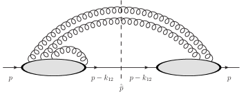
Figure 1: Double-real diagrams for the calculation of the quark beam function at N³LO.

We find it practical to construct the collinear limit of the relevant amplitude squared in fig. 1 by considering the Feynman diagrams for the process $q(p)\to q(q)+g(k_{1})+g(k_{2})\,.$ We employ QGRAF Nogueira:1991ex to generate all tree-level and one-loop diagrams, and use them to build up the amplitude in two independent implementations in FORM Vermaseren:2000nd and Mathematica. This requires care, since the quark $q(p)$ is on-shell, while the quark $q(q)$ is off-shell. This means that when one-loop corrections are generated, we must neglect all self-energy insertions on the on-shell external quark $q(p)$, but we need to include them on the off-shell quark $q(q)$.

As mentioned above, we need to use light-cone gauge for both real and virtual gluons. For example, when summing over real gluon polarizations, we obtain

$$\begin{split}&\sum_{pol}\,\epsilon_{i}^{\mu}(k_{i})\left(\epsilon_{i}^{\nu}(k_{i})\right)^{*}=-g^{\mu\nu}+\frac{k_{i}^{\mu}\bar{p}^{\nu}+k_{i}^{\nu}\bar{p}^{\mu}}{k_{i}\cdot\bar{p}}\,,\;\;\;i=1,2\,.\end{split}$$ (9)

Finally, we also need to use the axial gauge for virtual gluons, with the same reference vector $\bar{p}$. We note that the choice of $\bar{p}$ as the reference vector is convenient but not necessary.

We find 3 tree-level diagrams and 30 one-loop diagrams. Computing the interference, we obtain 90 “three-loop” phase-space diagrams. After performing the relevant Dirac algebra, each of these diagrams can be written as a linear combination of “three-loop” phase space integrals. We need to organize these integrals into integral families, in order to perform a reduction to master integrals using the well-known integration-by-parts identities Chetyrkin:1981qh . When dealing with phase space integrals subject to constraints, this step involves one more subtlety compared to what is done for standard multi-loop Feynman integrals. In order to understand this, we recall that a complete integral family should contain exactly as many propagators, as is the total number of independent scalar products that can be formed from the loop momenta and the external momenta. In our case, there are effectively three loop momenta and two external momenta ($p$ and $\bar{p}$); it follows that we can construct 12 independent scalar products. Therefore, we need to map our phase-space integrals to integral families with 12 independent propagators.

This requires some extra work. Indeed, consider again fig. 1. It is easy to convince oneself that, after Dirac algebra, the phase-space integrals stemming from these diagrams will have the following general form

$$\mathcal{I}\sim\int\frac{d^{d}k_{1}}{(2\pi)^{d-1}}\frac{d^{d}k_{2}}{(2\pi)^{d-1}}\frac{d^{d}k_{3}}{(2\pi)^{d}}\frac{\delta^{+\!\!}\left(k_{1}^{2}\right)\delta^{+\!\!}\left(k_{2}^{2}\right)\delta\left(p\cdot k_{12}-\tfrac{t}{2z}\right)\delta\left(\bar{p}\cdot k_{12}-\tfrac{1-z}{2}s\right)\,\mathcal{N}}{D_{1}^{n_{1}}\,D_{2}^{n_{2}}\,D_{3}^{n_{3}}\,D_{4}^{n_{4}}\,D_{5}^{n_{5}}\,D_{6}^{n_{6}}\,D_{7}^{n_{7}}\,D_{8}^{n_{8}}\,D_{9}^{n_{9}}\,D_{10}^{n_{10}}\,D_{11}^{n_{11}}\,}\,.$$ (10)

Here $k_{1},k_{2}$ are the momenta of two on-shell gluons and $k_{3}$ is the momentum of the virtual gluon. The $D_{j}$ are different, unspecified, denominators and $\mathcal{N}$ is a polynomial of scalar products of the loop momenta and the external momenta $p$, $\bar{p}$. It should be easy to see that the diagrams obtained from fig. 1 can generate at most 11 different propagators, including the combinations $k_{1}\cdot\bar{p}$ and $k_{2}\cdot\bar{p}$ which come from the sum over polarizations in eq. 9, along with similar denominator factors coming from the gluon propagators in axial gauge. Counting four delta-functions as “propagators” (we have in mind the reverse unitarity relation $\delta(x)\stackrel{{\scriptstyle\sim}}{{\to}}1/x$), we get 15 propagators in total. Since this number is larger than 12, the number of independent scalar products involving the momenta $k_{i}$, the propagators are linearly dependent and eq. 10 therefore does not constitute an integral family.

To remedy this problem, for every contributing diagram we partial fraction some of the linearly dependent propagators. For instance, we write

$$\frac{1}{(k_{1}\cdot\bar{p})(k_{2}\cdot\bar{p})}=\frac{2}{s(1-z)}\left[\frac{1}{k_{1}\cdot\bar{p}}+\frac{1}{k_{2}\cdot\bar{p}}\right],$$ (11)

$$\frac{1}{(k_{1}+k_{2})^{2}(k_{1}+k_{2}-p)^{2}}=\frac{z}{t}\left[\frac{1}{(k_{1}+k_{2}-p)^{2}}-\frac{1}{(k_{1}+k_{2})^{2}}\right],$$ (12)

$$\frac{1}{(k_{1}-p)^{2}(k_{2}-p)^{2}}=-\frac{z}{t}\left[\frac{1}{(k_{1}-p)^{2}}+\frac{1}{(k_{2}-p)^{2}}\right].$$ (13)

The partial fractioning effectively splits the diagrams into several terms, each of which contains at most 12 linearly independent propagators. At that point we can introduce well-defined integral families.

With this procedure we find that all diagrams can be expressed in terms of 19 independent integral families. The corresponding integrals can be written as

$$\mathcal{I}^{\text{top}}_{n_{1},\dotsc,n_{8}}=\int\frac{d^{d}k_{1}}{(2\pi)^{d-1}}\frac{d^{d}k_{2}}{(2\pi)^{d-1}}\frac{d^{d}k_{3}}{(2\pi)^{d}}\frac{\delta^{+\!\!}\left(k_{1}^{2}\right)\delta^{+\!\!}\left(k_{2}^{2}\right)\delta\left(p\cdot k_{12}-\tfrac{t}{2z}\right)\delta\left(\bar{p}\cdot k_{12}-\tfrac{1-z}{2}s\right)}{D_{1}^{n_{1}}\,D_{2}^{n_{2}}\,D_{3}^{n_{3}}\,D_{4}^{n_{4}}\,D_{5}^{n_{5}}\,D_{6}^{n_{6}}\,D_{7}^{n_{7}}\,D_{8}^{n_{8}}}\,,$$ (14)

where $\text{top}\in\{\text{A1},\text{A2},\dotsc,\text{A19}\}$ and the inverse propagators $D_{1},\dotsc,D_{8}$ for each integral family are shown in table 1.

top	$D_{1}$	$D_{2}$	$D_{3}$	$D_{4}$	$D_{5}$	$D_{6}$	$D_{7}$	$D_{8}$
A1	$k_{3}^{2}$	$k_{12}^{2}$	$k_{13}^{2}$	$k_{123}^{2}$	$(p-k_{1})^{2}$	$(p-k_{123})^{2}$	$\bar{p}\cdot k_{1}$	$\bar{p}\cdot k_{3}$
A2	$k_{3}^{2}$	$k_{13}^{2}$	$k_{123}^{2}$	$(p-k_{1})^{2}$	$(p-k_{12})^{2}$	$(p-k_{123})^{2}$	$\bar{p}\cdot k_{1}$	$\bar{p}\cdot k_{3}$
A3	$k_{3}^{2}$	$k_{12}^{2}$	$k_{13}^{2}$	$k_{123}^{2}$	$(p-k_{1})^{2}$	$(p-k_{123})^{2}$	$\bar{p}\cdot k_{2}$	$\bar{p}\cdot k_{3}$
A4	$k_{3}^{2}$	$k_{13}^{2}$	$k_{123}^{2}$	$(p-k_{1})^{2}$	$(p-k_{12})^{2}$	$(p-k_{123})^{2}$	$\bar{p}\cdot k_{2}$	$\bar{p}\cdot k_{3}$
A5	$k_{3}^{2}$	$k_{23}^{2}$	$(p-k_{1})^{2}$	$(p-k_{12})^{2}$	$(p-k_{23})^{2}$	$(p-k_{123})^{2}$	$\bar{p}\cdot k_{1}$	$\bar{p}\cdot k_{3}$
A6	$k_{3}^{2}$	$k_{13}^{2}$	$k_{123}^{2}$	$(p-k_{1})^{2}$	$(p-k_{12})^{2}$	$(p-k_{123})^{2}$	$\bar{p}\cdot k_{1}$	$\bar{p}\cdot k_{123}$
A7	$k_{3}^{2}$	$k_{12}^{2}$	$k_{13}^{2}$	$k_{123}^{2}$	$(p-k_{1})^{2}$	$(p-k_{13})^{2}$	$\bar{p}\cdot k_{1}$	$\bar{p}\cdot k_{3}$
A8	$k_{3}^{2}$	$k_{12}^{2}$	$k_{13}^{2}$	$k_{123}^{2}$	$(p-k_{1})^{2}$	$(p-k_{123})^{2}$	$\bar{p}\cdot k_{1}$	$\bar{p}\cdot k_{123}$
A9	$k_{3}^{2}$	$k_{12}^{2}$	$(p-k_{1})^{2}$	$(p-k_{3})^{2}$	$(p-k_{13})^{2}$	$(p-k_{123})^{2}$	$\bar{p}\cdot k_{1}$	$\bar{p}\cdot k_{3}$
A10	$k_{3}^{2}$	$k_{13}^{2}$	$(p-k_{1})^{2}$	$(p-k_{12})^{2}$	$(p-k_{13})^{2}$	$(p-k_{123})^{2}$	$\bar{p}\cdot k_{1}$	$\bar{p}\cdot k_{3}$
A11	$k_{3}^{2}$	$k_{12}^{2}$	$(p-k_{1})^{2}$	$(p-k_{3})^{2}$	$(p-k_{13})^{2}$	$(p-k_{123})^{2}$	$\bar{p}\cdot k_{2}$	$\bar{p}\cdot k_{3}$
A12	$k_{3}^{2}$	$(p-k_{1})^{2}$	$(p-k_{3})^{2}$	$(p-k_{12})^{2}$	$(p-k_{13})^{2}$	$(p-k_{123})^{2}$	$\bar{p}\cdot k_{1}$	$\bar{p}\cdot k_{3}$
A13	$k_{3}^{2}$	$(p-k_{1})^{2}$	$(p-k_{3})^{2}$	$(p-k_{12})^{2}$	$(p-k_{13})^{2}$	$(p-k_{123})^{2}$	$\bar{p}\cdot k_{2}$	$\bar{p}\cdot k_{3}$
A14	$k_{3}^{2}$	$k_{13}^{2}$	$(p-k_{1})^{2}$	$(p-k_{12})^{2}$	$(p-k_{13})^{2}$	$(p-k_{123})^{2}$	$\bar{p}\cdot k_{1}$	$\bar{p}\cdot k_{13}$
A15	$k_{3}^{2}$	$(p-k_{1})^{2}$	$(p-k_{3})^{2}$	$(p-k_{12})^{2}$	$(p-k_{23})^{2}$	$(p-k_{123})^{2}$	$\bar{p}\cdot k_{1}$	$\bar{p}\cdot k_{3}$
A16	$k_{3}^{2}$	$(p-k_{1})^{2}$	$(p-k_{3})^{2}$	$(p-k_{12})^{2}$	$(p-k_{23})^{2}$	$(p-k_{123})^{2}$	$\bar{p}\cdot k_{2}$	$\bar{p}\cdot k_{3}$
A17	$k_{3}^{2}$	$k_{12}^{2}$	$k_{23}^{2}$	$k_{123}^{2}$	$(p-k_{1})^{2}$	$(p-k_{123})^{2}$	$\bar{p}\cdot k_{1}$	$\bar{p}\cdot k_{3}$
A18	$k_{3}^{2}$	$k_{23}^{2}$	$k_{123}^{2}$	$(p-k_{1})^{2}$	$(p-k_{12})^{2}$	$(p-k_{123})^{2}$	$\bar{p}\cdot k_{1}$	$\bar{p}\cdot k_{3}$
A19	$k_{3}^{2}$	$k_{23}^{2}$	$k_{123}^{2}$	$(p-k_{1})^{2}$	$(p-k_{12})^{2}$	$(p-k_{123})^{2}$	$\bar{p}\cdot k_{1}$	$\bar{p}\cdot k_{123}$

Table 1: The inverse propagators $D_{i}$ for each of the 19 topologies A1, $\dotsc$, A19. Here we use the shorthand notation $k_{ij}=k_{i}+k_{j}$ and $k_{ij\ell}=k_{i}+k_{j}+k_{\ell}$.

For each integral family we perform the reduction to master integrals using Reduze 2 vonManteuffel:2012np , which supports operations with cut propagators. Performing the reduction, we find that all the contributing integrals can be expressed through 128 master integrals. We choose the set of master integrals as listed in table 2.

$\mathcal{I}^{\text{A1}}_{0,0,1,0,0,1,0,0}$	$\mathcal{I}^{\text{A1}}_{1,0,0,0,0,1,0,0}$	$\mathcal{I}^{\text{A1}}_{1,0,0,1,0,0,0,0}$	$\mathcal{I}^{\text{A1}}_{1,-1,0,0,0,1,0,0}$	$\mathcal{I}^{\text{A1}}_{0,0,1,0,0,1,0,1}$	$\mathcal{I}^{\text{A1}}_{1,0,1,0,0,1,0,0}$
$\mathcal{I}^{\text{A1}}_{-1,0,1,0,0,1,0,1}$	$\mathcal{I}^{\text{A1}}_{1,-1,1,0,0,1,0,0}$	$\mathcal{I}^{\text{A1}}_{0,1,1,0,0,1,0,1}$	$\mathcal{I}^{\text{A1}}_{0,1,1,0,0,1,1,0}$	$\mathcal{I}^{\text{A1}}_{1,0,0,0,1,1,1,0}$	$\mathcal{I}^{\text{A1}}_{1,0,0,1,0,1,0,1}$
$\mathcal{I}^{\text{A1}}_{1,0,1,0,0,1,0,1}$	$\mathcal{I}^{\text{A1}}_{1,0,1,0,0,1,1,0}$	$\mathcal{I}^{\text{A1}}_{-1,1,1,0,0,1,0,1}$	$\mathcal{I}^{\text{A1}}_{1,0,1,0,1,1,0,1}$	$\mathcal{I}^{\text{A1}}_{1,0,1,1,0,1,1,0}$	$\mathcal{I}^{\text{A1}}_{1,0,1,1,1,0,0,1}$
$\mathcal{I}^{\text{A1}}_{1,0,1,1,1,1,0,0}$	$\mathcal{I}^{\text{A1}}_{1,-1,1,0,1,1,0,1}$	$\mathcal{I}^{\text{A1}}_{1,0,1,-1,1,1,0,1}$	$\mathcal{I}^{\text{A1}}_{0,1,1,1,0,1,1,1}$	$\mathcal{I}^{\text{A2}}_{0,1,0,0,1,1,0,0}$	$\mathcal{I}^{\text{A2}}_{1,0,1,0,1,0,0,0}$
$\mathcal{I}^{\text{A2}}_{0,1,0,0,1,1,0,1}$	$\mathcal{I}^{\text{A2}}_{0,1,0,0,1,1,1,0}$	$\mathcal{I}^{\text{A2}}_{-1,1,0,0,1,1,0,1}$	$\mathcal{I}^{\text{A2}}_{0,1,-1,0,1,1,0,1}$	$\mathcal{I}^{\text{A2}}_{0,1,0,1,1,1,0,1}$	$\mathcal{I}^{\text{A2}}_{0,1,0,1,1,1,1,0}$
$\mathcal{I}^{\text{A2}}_{0,1,1,0,1,1,0,1}$	$\mathcal{I}^{\text{A2}}_{1,0,1,0,1,1,0,1}$	$\mathcal{I}^{\text{A2}}_{0,1,0,1,1,1,-1,1}$	$\mathcal{I}^{\text{A2}}_{0,1,1,0,1,1,1,1}$	$\mathcal{I}^{\text{A2}}_{1,1,1,0,1,1,1,0}$	$\mathcal{I}^{\text{A2}}_{1,1,1,1,1,0,0,1}$
$\mathcal{I}^{\text{A2}}_{1,1,1,1,1,1,0,0}$	$\mathcal{I}^{\text{A2}}_{1,1,1,-1,1,1,1,0}$	$\mathcal{I}^{\text{A2}}_{1,1,1,1,1,-1,0,1}$	$\mathcal{I}^{\text{A3}}_{1,0,0,0,1,1,1,0}$	$\mathcal{I}^{\text{A3}}_{1,0,0,1,1,0,1,0}$	$\mathcal{I}^{\text{A3}}_{1,0,1,0,0,1,1,0}$
$\mathcal{I}^{\text{A3}}_{1,0,1,0,0,1,1,1}$	$\mathcal{I}^{\text{A3}}_{1,0,1,0,1,1,1,0}$	$\mathcal{I}^{\text{A3}}_{1,0,1,1,0,0,1,1}$	$\mathcal{I}^{\text{A3}}_{1,0,1,1,0,1,1,0}$	$\mathcal{I}^{\text{A3}}_{1,1,0,0,1,1,1,0}$	$\mathcal{I}^{\text{A3}}_{1,0,1,0,1,1,1,1}$
$\mathcal{I}^{\text{A3}}_{1,1,0,1,1,1,1,1}$	$\mathcal{I}^{\text{A4}}_{0,1,0,0,1,1,1,0}$	$\mathcal{I}^{\text{A4}}_{0,1,0,1,1,1,1,0}$	$\mathcal{I}^{\text{A4}}_{1,0,1,1,1,0,1,0}$	$\mathcal{I}^{\text{A4}}_{1,1,1,0,1,0,1,1}$	$\mathcal{I}^{\text{A4}}_{1,1,1,0,1,1,1,0}$
$\mathcal{I}^{\text{A4}}_{1,1,1,-1,1,1,1,0}$	$\mathcal{I}^{\text{A5}}_{1,0,0,0,1,0,0,1}$	$\mathcal{I}^{\text{A5}}_{0,1,0,0,1,1,0,1}$	$\mathcal{I}^{\text{A5}}_{1,0,0,0,1,1,0,1}$	$\mathcal{I}^{\text{A5}}_{1,0,0,1,1,0,0,1}$	$\mathcal{I}^{\text{A5}}_{1,1,0,0,1,0,0,1}$
$\mathcal{I}^{\text{A5}}_{0,1,0,1,1,1,0,1}$	$\mathcal{I}^{\text{A5}}_{1,0,0,0,1,1,1,1}$	$\mathcal{I}^{\text{A5}}_{1,0,0,1,1,1,0,1}$	$\mathcal{I}^{\text{A5}}_{1,0,1,0,1,1,0,1}$	$\mathcal{I}^{\text{A5}}_{1,0,1,1,1,0,0,1}$	$\mathcal{I}^{\text{A5}}_{1,1,0,0,1,1,0,1}$
$\mathcal{I}^{\text{A5}}_{1,1,0,0,1,1,1,0}$	$\mathcal{I}^{\text{A5}}_{1,1,0,1,1,0,0,1}$	$\mathcal{I}^{\text{A5}}_{1,1,0,1,1,1,0,0}$	$\mathcal{I}^{\text{A5}}_{1,1,1,0,0,1,0,1}$	$\mathcal{I}^{\text{A5}}_{-1,1,0,1,1,1,0,1}$	$\mathcal{I}^{\text{A5}}_{0,1,-1,1,1,1,0,1}$
$\mathcal{I}^{\text{A5}}_{1,-1,1,0,1,1,0,1}$	$\mathcal{I}^{\text{A5}}_{1,1,-1,1,1,0,0,1}$	$\mathcal{I}^{\text{A5}}_{1,0,1,1,1,1,0,1}$	$\mathcal{I}^{\text{A5}}_{1,1,0,1,1,0,1,1}$	$\mathcal{I}^{\text{A5}}_{1,1,0,1,1,1,1,0}$	$\mathcal{I}^{\text{A5}}_{1,1,1,0,0,1,1,1}$
$\mathcal{I}^{\text{A5}}_{1,1,1,1,1,0,0,1}$	$\mathcal{I}^{\text{A5}}_{1,1,-1,1,1,1,1,0}$	$\mathcal{I}^{\text{A5}}_{1,1,1,1,1,0,1,1}$	$\mathcal{I}^{\text{A6}}_{1,1,1,0,1,0,1,1}$	$\mathcal{I}^{\text{A6}}_{1,1,1,1,1,0,0,1}$	$\mathcal{I}^{\text{A6}}_{1,1,1,1,1,-1,0,1}$
$\mathcal{I}^{\text{A7}}_{1,1,0,0,0,1,0,1}$	$\mathcal{I}^{\text{A8}}_{1,0,1,1,0,0,1,1}$	$\mathcal{I}^{\text{A8}}_{1,0,1,1,1,0,0,1}$	$\mathcal{I}^{\text{A9}}_{0,0,0,1,0,1,0,1}$	$\mathcal{I}^{\text{A9}}_{1,0,0,1,0,1,0,1}$	$\mathcal{I}^{\text{A9}}_{0,0,0,1,1,1,1,1}$
$\mathcal{I}^{\text{A9}}_{0,0,1,1,1,1,0,1}$	$\mathcal{I}^{\text{A9}}_{1,0,0,1,1,0,1,1}$	$\mathcal{I}^{\text{A9}}_{1,0,1,0,1,1,0,1}$	$\mathcal{I}^{\text{A9}}_{-1,0,1,1,1,1,0,1}$	$\mathcal{I}^{\text{A9}}_{1,0,0,1,1,1,1,1}$	$\mathcal{I}^{\text{A9}}_{1,0,1,0,1,1,1,1}$
$\mathcal{I}^{\text{A9}}_{1,1,1,0,1,1,0,1}$	$\mathcal{I}^{\text{A9}}_{1,1,1,-1,1,1,0,1}$	$\mathcal{I}^{\text{A10}}_{0,1,0,1,1,1,1,1}$	$\mathcal{I}^{\text{A10}}_{0,1,1,1,1,1,0,1}$	$\mathcal{I}^{\text{A10}}_{0,1,1,1,1,1,1,1}$	$\mathcal{I}^{\text{A11}}_{0,0,0,1,1,1,1,1}$
$\mathcal{I}^{\text{A11}}_{0,0,1,1,0,1,1,1}$	$\mathcal{I}^{\text{A11}}_{1,0,0,1,1,1,1,1}$	$\mathcal{I}^{\text{A11}}_{1,0,1,1,0,1,1,1}$	$\mathcal{I}^{\text{A11}}_{1,1,0,1,1,0,1,1}$	$\mathcal{I}^{\text{A11}}_{1,1,1,1,0,1,1,1}$	$\mathcal{I}^{\text{A12}}_{0,0,1,1,0,1,0,1}$
$\mathcal{I}^{\text{A12}}_{1,0,1,1,1,0,0,1}$	$\mathcal{I}^{\text{A12}}_{0,1,1,1,1,1,0,1}$	$\mathcal{I}^{\text{A12}}_{-1,1,1,1,1,1,0,1}$	$\mathcal{I}^{\text{A13}}_{1,0,1,1,1,0,1,1}$	$\mathcal{I}^{\text{A14}}_{0,1,1,1,1,1,0,1}$	$\mathcal{I}^{\text{A14}}_{0,1,1,1,1,1,1,1}$
$\mathcal{I}^{\text{A15}}_{0,1,1,0,1,1,0,1}$	$\mathcal{I}^{\text{A15}}_{-1,1,1,0,1,1,0,1}$	$\mathcal{I}^{\text{A15}}_{0,1,1,1,1,1,0,1}$	$\mathcal{I}^{\text{A15}}_{1,1,1,0,1,1,0,1}$	$\mathcal{I}^{\text{A15}}_{-1,1,1,1,1,1,0,1}$	$\mathcal{I}^{\text{A16}}_{1,1,1,0,1,1,1,1}$
$\mathcal{I}^{\text{A17}}_{1,0,1,1,1,0,0,1}$	$\mathcal{I}^{\text{A17}}_{1,1,1,0,1,1,0,1}$	$\mathcal{I}^{\text{A17}}_{1,1,1,-1,1,1,0,1}$	$\mathcal{I}^{\text{A18}}_{1,1,1,1,1,0,0,1}$	$\mathcal{I}^{\text{A18}}_{1,1,1,1,1,-1,0,1}$	$\mathcal{I}^{\text{A19}}_{1,1,1,1,0,0,0,1}$
$\mathcal{I}^{\text{A19}}_{1,1,1,1,1,0,0,1}$	$\mathcal{I}^{\text{A19}}_{1,1,1,1,1,-1,0,1}$

Table 2: The set of 128 master integrals for the matching coefficients of the double-real contribution to the quark beam function.

In the next section we discuss in detail how to evaluate these 128 master integrals using the method of differential equations Kotikov:1990kg ; Bern:1993kr ; Remiddi:1997ny ; Gehrmann:1999as augmented by the use of a canonical basis Henn:2013pwa .

3 Master integrals

Having expressed the amplitude in terms of master integrals, we proceed with the discussion of their evaluation. The master integrals depend on the three quantities $s=2p\cdot\bar{p}$, $\,t$ and $z$, cf. eq. 14. However, some of these dependencies are quite simple. Indeed, we re-define the gluon momenta as $k_{i}={\tilde{k}}_{i}\,\sqrt{t/z},~{}p={\tilde{p}}\,\sqrt{t/z}$ and $\bar{p}={\tilde{\bar{p}}}\,s\sqrt{z/t}$. Since $p\cdot\bar{p}=s/2$, we find ${\tilde{p}}\cdot{\tilde{\bar{p}}}=1/2$. Applying these transformations to integrands of master integrals, we find

$$\mathcal{I}^{\text{top}}_{n_{1},\dotsc,n_{8}}(s,t,z) =\left(\frac{1}{s}\right)^{1+n_{7}+n_{8}}\left(\frac{t}{z}\right)^{3-(n_{1}+n_{2}+\dotsc+n_{6})-3\epsilon}\mathcal{I}^{\text{top}}_{n_{1},\dotsc,n_{8}}(1,z,z)\,,$$ (15)

$$\equiv\left(\frac{1}{s}\right)^{1+n_{7}+n_{8}}\left(\frac{t}{z}\right)^{3-(n_{1}+n_{2}+\dotsc+n_{6})-3\epsilon}\mathcal{I}^{\text{top}}_{n_{1},\dotsc,n_{8}}(z)\,.$$ (16)

Note that the second step in the above equation implies that one can get the expression for the re-scaled integral upon taking the definition of the original integral with its full $s,t$ and $z$ dependence and then evaluating it for $s=1$ and $t=z$.

In order to calculate the master integrals $\mathcal{I}^{\text{top}}_{n_{1},\dotsc,n_{8}}(z)$ on the right-hand side of eq. 16, we compute their derivative with respect to $z$ and re-express the result in terms of master integrals by means of integration-by-parts reduction, thus producing a closed system of differential equations. We write it as

$$\frac{d}{dz}\vec{\mathcal{I}}(z,\epsilon)=\hat{A}(z,\epsilon)\,\vec{\mathcal{I}}(z,\epsilon)\,,$$ (17)

where $\vec{\mathcal{I}}(z,\epsilon)$ contains the $128$ master integrals in table 2 with $s=1$ and $t=z$, and $\hat{A}(z,\epsilon)$ is a $128\times 128$ matrix. We use the program Fuchsia Gituliar:2017vzm to transform the system of equation to the $\epsilon$-form using the algorithm described in ref. Lee:2014ioa . We find

$$\frac{d}{dz}\vec{\mathcal{I}}_{\text{can}}(z,\epsilon)=\epsilon\,\left(\frac{\hat{A}_{-1}}{z+1}+\frac{\hat{A}_{0}}{z}+\frac{\hat{A}_{1}}{z-1}+\frac{\hat{A}_{2}}{z-2}\right)\vec{\mathcal{I}}_{\text{can}}(z,\epsilon)\,,$$ (18)

where the $\hat{A}_{k}$ are constant matrices. The vector $\vec{\mathcal{I}}_{\text{can}}(z,\epsilon)$ contains the canonical master integrals; it is related to the original master integrals $\vec{\mathcal{I}}(z,\epsilon)=\hat{T}(z,\epsilon)\,\vec{\mathcal{I}}_{\text{can}}(z,\epsilon)$ by a transformation matrix $\hat{T}(z,\epsilon)$.

The system of differential equations in eq. 18 is solved iteratively for the coefficients of $\vec{\mathcal{I}}_{\text{can}}(z,\epsilon)$ in an expansion around $\epsilon=0$. The result of this procedure can be written as

$$\vec{\mathcal{I}}_{\text{can}}(z,\epsilon)=\hat{M}(z,\epsilon)\,\vec{B}(\epsilon)\,,$$ (19)

where the $128\times 128$ matrix $\hat{M}(z,\epsilon)$ contains elements of the form

$$M_{ij}(z,\epsilon)=\sum_{k=0}^{6}\,\sum_{\vec{w}\,\in\,W(k)}c_{i,j,k,\vec{w}}\,\,\epsilon^{k}\,G(\vec{w};z)\,.$$ (20)

The inner sum runs over vectors $\vec{w}$ of length $k$ whose components are drawn from a set $\{-1,0,1,2\}$, which are the singular points in the differential equations eq. 18. The $G(\vec{w};z)$ are multiple polylogarithms Goncharov:1998kja ; Remiddi:1999ew ; Goncharov:2001iea ; Vollinga:2004sn , which are defined iteratively as

$$G(w_{1},w_{2},\dotsc,w_{n};z)=\int_{0}^{z}dt\,\frac{G(w_{2},w_{3},\dotsc,w_{n};t)}{t-w_{1}}\,,$$ (21)

with the special cases

$$G(;z)=1~{},~{}~{}~{}G(\underbrace{0,\dotsc,0}_{n\,\text{times}};z)=\frac{1}{n!}\log^{n}(z)\,.$$ (22)

The constant vector $\vec{B}(\epsilon)$ in eq. 19 is fixed by the boundary conditions required for the solution of the system of first-order differential equations. We extract the boundary condition from the behaviour of the master integrals in the limit $z\to 1$.

In principle, it is possible to extract the boundary conditions by writing

$$\vec{\mathcal{I}}(z,\epsilon)=\hat{T}(z,\epsilon)\,\hat{M}(z,\epsilon)\,\vec{B}(\epsilon)\,,$$ (23)

and taking the limit $z\to 1$. The multiple polylogarithms $G(\vec{w};z)$ inside $\hat{M}(z,\epsilon)$, appearing on the right-hand side of eq. 23, are, in general, logarithmically divergent in this limit. This divergence should be extracted by writing the multiple polylogarithms in the form $G(\vec{w};z)=\sum_{\ell}c_{\ell}\log^{\ell}(1-z)$. Computing a sufficient number of integrals $\vec{\mathcal{I}}(z,\epsilon)$ that appear on the left-hand side of eq. 23 in the $z\to 1$ limit allows to determine the constants $\vec{B}(\epsilon)$.

In performing the computation of the master integrals we should remember that the beam function matching coefficients should be treated as distributions in $(1-z)$. Indeed, the matching coefficients have to be convoluted with the PDFs and all divergences in the limit $z\to 1$ have to be regularized, extracted and renormalized in order to obtain the final finite result in terms of quantities like $\delta(1-z)$, $[1/(1-z)]_{+}$, etc. To extract these distributions, one needs to have the master integrals written in the “resummed” form, i.e. the $\epsilon$ dependence in the limit $z\to 1$ has to be made explicit in the form of $(1-z)^{a+b\epsilon}$ powers. It is convenient, therefore, to extract the boundary constants in a similar way, namely by matching equal powers of $(1-z)^{\epsilon}$ on both sides of eq. 23.

In order to do that, the right-hand side of eq. 23 should first be written in the “resummed” form $\sum_{\ell,m}c_{\ell,m}(\epsilon)(1-z)^{n+\ell\epsilon}\log^{m}(1-z)$, which can be easily achieved by solving the differential equations in eq. 18 in the limit $z\to 1$

$$\frac{d}{dz}\vec{\mathcal{I}}_{\text{can}}(z\to 1,\epsilon)=\epsilon\,\frac{\hat{A}_{1}}{z-1}\,\vec{\mathcal{I}}_{\text{can}}(z\to 1,\epsilon)\,,$$ (24)

whose solution is given by a matrix exponential

$$\vec{\mathcal{I}}_{\text{can}}(z\to 1,\epsilon)=(1-z)^{-\epsilon\hat{A}_{1}}\vec{H}(\epsilon)\,.$$ (25)

The new constants in $\vec{H}(\epsilon)$ can be expressed as linear combinations of the constants in $\vec{B}(\epsilon)$ by equating the right-hand side of eq. 19 taken in the limit $z\to 1$ and the right-hand side of eq. 25 expanded in $\epsilon$. Multiplying both sides in eq. 25 by the transformation matrix $\hat{T}(z,\epsilon)$ in the limit $z\to 1$ and performing the matrix exponentiation gives the leading-power behaviour of the master integrals

$$\mathcal{I}^{(i)}(z\to 1,\epsilon)=\sum_{\ell=-3}^{2}\sum_{m=0}^{2}C_{i,\ell,m}(\epsilon)\,(1-z)^{n(i)+\ell\epsilon}\log^{m}(1-z)\,,~{}~{}(i=1,\dotsc,128;~{}n(i)\in\mathbb{Z})\,.$$ (26)

The coefficients $C_{i,\ell,m}(\epsilon)$ are in general linear combinations of the $128$ constants in $\vec{B}(\epsilon)$. Therefore, we need to compute sufficiently many linearly independent $C_{i,\ell,m}(\epsilon)$ to determine all boundary constants. Fortunately, we can fix many boundary constants by identifying the constants $C_{i,\ell,m}(\epsilon)$ that must vanish in order to produce the correct behaviour of the master integrals in the limit $z\to 1$.

As an explicit example, consider the second master integral $\mathcal{I}^{(2)}(z\to 1)=\mathcal{I}^{\text{A1}}_{1,0,0,0,0,1,0,0}|_{z\to 1}$. On the one hand, the differential equations predict that in the limit $z\to 1$ the integral has the form

$$\mathcal{I}^{(2)}(z\to 1)=C_{2,0,0}(\epsilon)+C_{2,-2,0}(\epsilon)(1-z)^{-2\epsilon}+\mathcal{O}(1-z)\,.$$ (27)

On the other hand, its integral representation suggests that its leading behaviour scales as $(1-z)^{1-2\epsilon}$, which implies that $C_{2,0,0}(\epsilon)=C_{2,-2,0}(\epsilon)=0$. Let us verify this by inspecting the integral representation

$$\mathcal{I}^{(2)}(z\to 1)=\int\frac{d^{d}k_{1}}{(2\pi)^{d-1}}\frac{d^{d}k_{2}}{(2\pi)^{d-1}}\frac{d^{d}k_{3}}{(2\pi)^{d}}\frac{\delta^{+\!\!}\left(k_{1}^{2}\right)\delta^{+\!\!}\left(k_{2}^{2}\right)\delta\left(p\cdot k_{12}-\tfrac{1}{2}\right)\delta\left(\bar{p}\cdot k_{12}-\tfrac{1-z}{2}\right)}{k_{3}^{2}\,(p-k_{123})^{2}}\,.$$ (28)

The integral over $k_{3}$ is straightforward to evaluate. The result is proportional to ${[-(p-k_{12})^{2}]^{-\epsilon}}$ which becomes $[1-k_{12}^{2}]^{-\epsilon}$ upon imposing the delta-function $\delta(p\cdot k_{12}-\tfrac{1}{2})$ and the on-shellness $p^{2}=0$ constraints. The last delta-function in the numerator of eq. 28 fixes the projection of the total emitted momentum $k_{12}\equiv k_{1}+k_{2}$ to be small in the limit $z\to 1$. To capture that, it is convenient to make a Sudakov decomposition of $k_{1}$ and $k_{2}$

$$k_{i}^{\mu}=\alpha_{i}\,p^{\mu}+\beta_{i}\,\bar{p}^{\mu}+k_{i\perp}^{\mu}\,.$$ (29)

We use this decomposition to compute $2\bar{p}\cdot k_{12}=\alpha_{12}\equiv\alpha_{1}+\alpha_{2}\sim\mathcal{O}\left(1-z\right)$ and $2p\cdot k_{12}=\beta_{12}\equiv\beta_{1}+\beta_{2}\sim\mathcal{O}\left(1\right)$. Moreover, the fact that the momenta $k_{1}$ and $k_{2}$ are both on-shell and have positive energy, implies that $\alpha_{i}\sim\mathcal{O}\left(1-z\right),\beta_{i}\sim\mathcal{O}\left(1\right)$ and $k_{i\perp}^{2}\sim\mathcal{O}\left(1-z\right)$ for $i=1,2$ separately. As a consequence, $k_{12}^{2}\sim\mathcal{O}\left(1-z\right)$ and the result of the $k_{3}$ integral can be simplified $[1-k_{12}^{2}]^{-\epsilon}=1+\mathcal{O}\left(1-z\right)$. The integration measures for $k_{1}$ and $k_{2}$ reads $d^{d}k_{i}=\frac{1}{4}\,d\alpha_{i}\,d\beta_{i}\,d(k_{i\perp}^{2})\,(k_{i\perp}^{2})^{-\epsilon}\,d\Omega_{i}^{(d-2)}$ and scale as $\mathcal{O}\left((1-z)^{2-\epsilon}\right)$. Three of the delta functions in eq. 28 scale as $\mathcal{O}\left((1-z)^{-1}\right)$. Putting everything together, we find that $\mathcal{I}^{(2)}(z\to 1)=\mathcal{O}\left((1-z)^{1-2\epsilon}\right)$. Therefore, there are no contributions to the integral that scale as $\mathcal{O}\left((1-z)^{0}\right)$ or $\mathcal{O}\left((1-z)^{-2\epsilon}\right)$. We conclude that the coefficients of these regions vanish: $C_{2,0,0}(\epsilon)=C_{2,-2,0}(\epsilon)=0$.

After finding all the coefficients $C_{i,\ell,m}(\epsilon)$ that must vanish because of similar arguments, we acquire enough relations to express 104 of the boundary constants in $\vec{B}(\epsilon)$ in terms of a remaining set of 24 constants. To determine the latter constants we performed explicit computations of non-vanishing regions of selected master integrals in the limit $z\to 1$.

The boundary integrals that we have calculated are

$$B_{1}=\mathcal{I}_{0,0,1,0,0,1,0,0}^{\text{A1}}\big{|}_{s=1,t=z,z\approx 1} =C_{1,-2,0}(\epsilon)(1-z)^{1-2\epsilon}~{},$$ (30)

$$B_{2}=\mathcal{I}_{1,0,0,1,0,0,0,0}^{\text{A1}}\big{|}_{s=1,t=z,z\approx 1} =C_{3,-3,0}(\epsilon)(1-z)^{1-3\epsilon}~{},$$ (31)

$$B_{3}=\mathcal{I}_{0,0,1,0,0,1,0,1}^{\text{A1}}\big{|}_{s=1,t=z,z\approx 1} =C_{5,-3,0}(\epsilon)(1-z)^{1-3\epsilon}~{},$$ (32)

$$B_{4}=\mathcal{I}_{0,1,1,0,0,1,0,1}^{\text{A1}}\big{|}_{s=1,t=z,z\approx 1} =C_{9,-3,0}(\epsilon)(1-z)^{-3\epsilon}~{},$$ (33)

$$B_{5}=\mathcal{I}_{0,1,1,0,0,1,1,0}^{\text{A1}}\big{|}_{s=1,t=z,z\approx 1} =C_{10,-2,0}(\epsilon)(1-z)^{-1-2\epsilon}~{},$$ (34)

$$B_{6}=\mathcal{I}_{1,0,0,1,0,1,0,1}^{\text{A1}}\big{|}_{s=1,t=z,z\approx 1} =C_{12,-3,0}(\epsilon)(1-z)^{-3\epsilon}~{},$$ (35)

$$B_{7}=\mathcal{I}_{1,0,1,0,1,1,0,1}^{\text{A1}}\big{|}_{s=1,t=z,z\approx 1} =C_{16,-3,0}(\epsilon)(1-z)^{-3\epsilon}~{},$$ (36)

$$B_{8}=\mathcal{I}_{1,0,1,1,0,1,1,0}^{\text{A1}}\big{|}_{s=1,t=z,z\approx 1} =C_{17,-3,0}(\epsilon)(1-z)^{-1-3\epsilon}~{},$$ (37)

$$B_{9}=\mathcal{I}_{1,0,1,1,1,0,0,1}^{\text{A1}}\big{|}_{s=1,t=z,z\approx 1} =C_{18,-3,0}(\epsilon)(1-z)^{-1-3\epsilon}~{},$$ (38)

$$B_{10}=\mathcal{I}_{1,0,1,1,1,1,0,0}^{\text{A1}}\big{|}_{s=1,t=z,z\approx 1} =C_{19,-3,0}(\epsilon)(1-z)^{-3\epsilon}~{},$$ (39)

$$B_{11}=\mathcal{I}_{0,1,1,1,0,1,1,1}^{\text{A1}}\big{|}_{s=1,t=z,z\approx 1} =C_{22,-3,0}(\epsilon)(1-z)^{-2-3\epsilon}~{},$$ (40)

$$B_{12}=\mathcal{I}_{1,0,0,1,1,0,1,0}^{\text{A3}}\big{|}_{s=1,t=z,z\approx 1} =C_{41,-3,0}(\epsilon)(1-z)^{-3\epsilon}~{},$$ (41)

$$B_{13}=\mathcal{I}_{1,0,1,0,1,1,1,0}^{\text{A3}}\big{|}_{s=1,t=z,z\approx 1} =C_{44,-2,0}(\epsilon)(1-z)^{-2\epsilon}~{},$$ (42)

$$B_{14}=\mathcal{I}_{1,0,1,1,0,0,1,1}^{\text{A3}}\big{|}_{s=1,t=z,z\approx 1} =C_{45,-3,0}(\epsilon)(1-z)^{-2-3\epsilon}~{},$$ (43)

$$B_{15}=\mathcal{I}_{1,0,1,1,0,1,1,0}^{\text{A3}}\big{|}_{s=1,t=z,z\approx 1} =C_{46,-3,0}(\epsilon)(1-z)^{-1-3\epsilon}~{},$$ (44)

$$B_{16}=\mathcal{I}_{1,1,0,0,1,1,1,0}^{\text{A3}}\big{|}_{s=1,t=z,z\approx 1} =C_{47,-2,0}(\epsilon)(1-z)^{-1-2\epsilon}~{},$$ (45)

$$B_{17}=\mathcal{I}_{1,1,0,1,1,1,1,1}^{\text{A3}}\big{|}_{s=1,t=z,z\approx 1} =C_{49,-3,0}(\epsilon)(1-z)^{-2-3\epsilon}~{},$$ (46)

$$B_{18}=\mathcal{I}_{1,1,0,0,1,0,0,1}^{\text{A5}}\big{|}_{s=1,t=z,z\approx 1} =C_{60,-3,0}(\epsilon)(1-z)^{-3\epsilon}~{},$$ (47)

$$B_{19}=\mathcal{I}_{1,1,0,0,1,1,1,0}^{\text{A5}}\big{|}_{s=1,t=z,z\approx 1} =C_{67,-2,0}(\epsilon)(1-z)^{-2\epsilon}~{},$$ (48)

$$B_{20}=\mathcal{I}_{1,0,1,1,0,0,1,1}^{\text{A8}}\big{|}_{s=1,t=z,z\approx 1} =C_{86,-3,0}(\epsilon)(1-z)^{-2-3\epsilon}~{},$$ (49)

$$B_{21}=\mathcal{I}_{1,0,1,1,1,0,0,1}^{\text{A8}}\big{|}_{s=1,t=z,z\approx 1} =C_{87,-3,0}(\epsilon)(1-z)^{-1-3\epsilon}~{},$$ (50)

$$B_{22}=\mathcal{I}_{1,0,1,1,1,0,0,1}^{\text{A17}}\big{|}_{s=1,t=z,z\approx 1} =C_{121,-3,0}(\epsilon)(1-z)^{-1-3\epsilon}~{},$$ (51)

$$B_{23}=\mathcal{I}_{1,1,1,0,1,1,0,1}^{\text{A17}}\big{|}_{s=1,t=z,z\approx 1} =C_{122,-3,0}(\epsilon)(1-z)^{-1-3\epsilon}~{},$$ (52)

$$B_{24}=\mathcal{I}_{1,1,1,1,0,0,0,1}^{\text{A19}}\big{|}_{s=1,t=z,z\approx 1} =C_{126,-3,0}(\epsilon)(1-z)^{-1-3\epsilon}~{}.$$ (53)

In the following, we provide the results for these constants and present a few examples that illustrate how they are evaluated.

3.1 Results for explicitly calculated coefficients

Here we list the results in terms of Laurent series in $\epsilon$ for the constants $C_{i,j,k}(\epsilon)$ that appear in eqs. 30 to 53. In the following sections we provide the reader with some examples of the computations that led to the expressions listed below. For convenience we extract a common $\epsilon$-dependent pre-factor,

$$C_{i,j,k}(\epsilon)=i\left(\frac{\Omega_{d-2}}{(2\pi)^{d-1}}\right)^{3}\widetilde{C}_{i,j,k}(\epsilon)\,.$$ (54)

The results for the constants, up to weight six, are

$$\widetilde{C}_{1,-2,0}(\epsilon) =\tfrac{1}{(1-3\epsilon)(1-2\epsilon)^{2}}\left(\tfrac{1}{16\epsilon}-\tfrac{\pi^{2}\epsilon}{32}-\tfrac{5\zeta_{3}\epsilon^{2}}{8}-\tfrac{\pi^{4}\epsilon^{3}}{128}+\left(\tfrac{5\pi^{2}\zeta_{3}}{16}-\tfrac{27\zeta_{5}}{8}\right)\epsilon^{4}\right.$$

$$\left.+\left(\tfrac{25\zeta_{3}^{2}}{8}-\tfrac{521\pi^{6}}{241920}\right)\epsilon^{5}+\mathcal{O}\left(\epsilon^{6}\right)\right),$$ (55)

$$\widetilde{C}_{3,-3,0}(\epsilon) =\tfrac{e^{i\pi\epsilon}}{(1-3\epsilon)(1-2\epsilon)^{2}}\left(\tfrac{1}{16\epsilon}-\tfrac{\pi^{2}\epsilon}{32}-\tfrac{5\zeta_{3}\epsilon^{2}}{8}-\tfrac{\pi^{4}\epsilon^{3}}{128}+\left(\tfrac{5\pi^{2}\zeta_{3}}{16}-\tfrac{27\zeta_{5}}{8}\right)\epsilon^{4}\right.$$

$$\left.+\left(\tfrac{25\zeta_{3}^{2}}{8}-\tfrac{521\pi^{6}}{241920}\right)\epsilon^{5}+\mathcal{O}\left(\epsilon^{6}\right)\right),$$ (56)

$$\widetilde{C}_{5,-3,0}(\epsilon) =\tfrac{e^{i\pi\epsilon}}{(1-3\epsilon)^{2}}\left(\tfrac{1}{8\epsilon^{2}}-\tfrac{\pi^{2}}{24}-\tfrac{3\zeta_{3}\epsilon}{2}-\tfrac{13\pi^{4}\epsilon^{2}}{360}+\left(\tfrac{\pi^{2}\zeta_{3}}{2}-\tfrac{21\zeta_{5}}{2}\right)\epsilon^{3}\right.$$

$$\left.+\left(9\zeta_{3}^{2}-\tfrac{59\pi^{6}}{3780}\right)\epsilon^{4}+\mathcal{O}\left(\epsilon^{5}\right)\right),$$ (57)

$$\widetilde{C}_{9,-3,0}(\epsilon) =\tfrac{e^{i\pi\epsilon}}{1-4\epsilon}\left(-\tfrac{1}{8\epsilon^{3}}+\tfrac{\pi^{2}}{16\epsilon}+\tfrac{19\zeta_{3}}{8}+\tfrac{41\pi^{4}\epsilon}{576}+\left(\tfrac{423\zeta_{5}}{16}-\tfrac{29\pi^{2}\zeta_{3}}{24}\right)\epsilon^{2}\right.$$

$$\left.+\left(\tfrac{1273\pi^{6}}{24192}-23\zeta_{3}^{2}\right)\epsilon^{3}+\mathcal{O}\left(\epsilon^{4}\right)\right),$$ (58)

$$\widetilde{C}_{10,-2,0}(\epsilon) =\tfrac{1}{1-2\epsilon}\left(\tfrac{1}{8\epsilon^{3}}-\tfrac{\pi^{2}}{12\epsilon}-2\zeta_{3}-\tfrac{53\pi^{4}\epsilon}{1440}+\left(\tfrac{29\pi^{2}\zeta_{3}}{24}-\tfrac{129\zeta_{5}}{8}\right)\epsilon^{2}\right.$$

$$\left.+\left(\tfrac{55\zeta_{3}^{2}}{4}-\tfrac{341\pi^{6}}{20160}\right)\epsilon^{3}+\mathcal{O}\left(\epsilon^{4}\right)\right),$$ (59)

$$\widetilde{C}_{12,-3,0}(\epsilon) =\tfrac{e^{i\pi\epsilon}}{1-2\epsilon}\left(-\tfrac{\pi^{2}}{24\epsilon}-\tfrac{3\zeta_{3}}{4}-\tfrac{19\pi^{4}\epsilon}{1440}+\left(\tfrac{19\pi^{2}\zeta_{3}}{24}-\tfrac{75\zeta_{5}}{8}\right)\epsilon^{2}\right.$$

$$\left.+\left(\tfrac{15\zeta_{3}^{2}}{2}-\tfrac{547\pi^{6}}{60480}\right)\epsilon^{3}+\mathcal{O}\left(\epsilon^{4}\right)\right),$$ (60)

$$\widetilde{C}_{16,-3,0}(\epsilon) =e^{i\pi\epsilon}\left(-\tfrac{1}{16\epsilon^{4}}+\tfrac{\zeta_{3}}{8\epsilon}+\tfrac{\pi^{4}}{960}+\left(\tfrac{\pi^{2}\zeta_{3}}{8}-\tfrac{9\zeta_{5}}{16}\right)\epsilon+\left(\tfrac{7\zeta_{3}^{2}}{4}+\tfrac{227\pi^{6}}{120960}\right)\epsilon^{2}+\mathcal{O}\left(\epsilon^{3}\right)\right),$$ (61)

$$\widetilde{C}_{17,-3,0}(\epsilon) =e^{i\pi\epsilon}\left(-\tfrac{5}{16\epsilon^{4}}+\tfrac{11\pi^{2}}{32\epsilon^{2}}+\tfrac{11\zeta_{3}}{\epsilon}+\tfrac{193\pi^{4}}{640}+\left(\tfrac{549\zeta_{5}}{4}-\tfrac{17\pi^{2}\zeta_{3}}{2}\right)\epsilon\right.$$

$$\left.+\left(\tfrac{47227\pi^{6}}{241920}-118\zeta_{3}^{2}\right)\epsilon^{2}+\mathcal{O}\left(\epsilon^{3}\right)\right),$$ (62)

$$\widetilde{C}_{18,-3,0}(\epsilon) =\tfrac{e^{i\pi\epsilon}}{1+4\epsilon}\left(\tfrac{19}{32\epsilon^{3}}-\tfrac{19\pi^{2}}{64\epsilon}-\tfrac{77\zeta_{3}}{16}+\tfrac{49\pi^{4}\epsilon}{1280}+\left(\tfrac{77\pi^{2}\zeta_{3}}{32}+\tfrac{441\zeta_{5}}{16}\right)\epsilon^{2}\right.$$

$$\left.+\left(\tfrac{403\zeta_{3}^{2}}{16}+\tfrac{21953\pi^{6}}{96768}\right)\epsilon^{3}+\mathcal{O}\left(\epsilon^{4}\right)\right),$$ (63)

$$\widetilde{C}_{19,-3,0}(\epsilon) =e^{i\pi\epsilon}\left(\tfrac{3}{32\epsilon^{4}}-\tfrac{11\pi^{2}}{192\epsilon^{2}}-\tfrac{5\zeta_{3}}{4\epsilon}-\tfrac{199\pi^{4}}{11520}+\left(\tfrac{17\pi^{2}\zeta_{3}}{24}-\tfrac{59\zeta_{5}}{8}\right)\epsilon\right.$$

$$\left.+\left(\tfrac{15\zeta_{3}^{2}}{2}-\tfrac{775\pi^{6}}{290304}\right)\epsilon^{2}+\mathcal{O}\left(\epsilon^{3}\right)\right),$$ (64)

$$\widetilde{C}_{22,-3,0}(\epsilon) =e^{i\pi\epsilon}\left(\tfrac{11}{16\epsilon^{4}}-\tfrac{13\pi^{2}}{48\epsilon^{2}}-\tfrac{17\zeta_{3}}{2\epsilon}-\tfrac{83\pi^{4}}{480}+\left(\tfrac{35\pi^{2}\zeta_{3}}{12}-\tfrac{387\zeta_{5}}{8}\right)\epsilon\right.$$

$$\left.+\left(\tfrac{181\zeta_{3}^{2}}{4}-\tfrac{3457\pi^{6}}{60480}\right)\epsilon^{2}+\mathcal{O}\left(\epsilon^{3}\right)\right),$$ (65)

$$\widetilde{C}_{41,-3,0}(\epsilon) =\tfrac{e^{i\pi\epsilon}}{1-2\epsilon}\left(-\tfrac{1}{8\epsilon^{3}}+\tfrac{\pi^{2}}{12\epsilon}+2\zeta_{3}+\tfrac{53\pi^{4}\epsilon}{1440}+\left(\tfrac{129\zeta_{5}}{8}-\tfrac{29\pi^{2}\zeta_{3}}{24}\right)\epsilon^{2}\right.$$

$$\left.+\left(\tfrac{341\pi^{6}}{20160}-\tfrac{55\zeta_{3}^{2}}{4}\right)\epsilon^{3}+\mathcal{O}\left(\epsilon^{4}\right)\right),$$ (66)

$$\widetilde{C}_{44,-2,0}(\epsilon) =\tfrac{1}{1+\epsilon}\left(-\tfrac{1}{8\epsilon^{3}}+\tfrac{5\pi^{2}}{48\epsilon}+\tfrac{9\zeta_{3}}{4}+\tfrac{19\pi^{4}\epsilon}{576}+\left(\tfrac{63\zeta_{5}}{4}-\tfrac{11\pi^{2}\zeta_{3}}{8}\right)\epsilon^{2}\right.$$

$$\left.+\left(\tfrac{101\pi^{6}}{8064}-\tfrac{57\zeta_{3}^{2}}{4}\right)\epsilon^{3}+\mathcal{O}\left(\epsilon^{4}\right)\right),$$ (67)

$$\widetilde{C}_{45,-3,0}(\epsilon) =e^{i\pi\epsilon}\left(-\tfrac{3}{8\epsilon^{4}}+\tfrac{11\pi^{2}}{48\epsilon^{2}}+\tfrac{5\zeta_{3}}{\epsilon}+\tfrac{199\pi^{4}}{2880}+\left(\tfrac{59\zeta_{5}}{2}-\tfrac{17\pi^{2}\zeta_{3}}{6}\right)\epsilon\right.$$

$$\left.+\left(\tfrac{775\pi^{6}}{72576}-30\zeta_{3}^{2}\right)\epsilon^{2}+\mathcal{O}\left(\epsilon^{3}\right)\right),$$ (68)

$$\widetilde{C}_{46,-3,0}(\epsilon) =\tfrac{e^{i\pi\epsilon}}{1+4\epsilon}\left(-\tfrac{19}{32\epsilon^{3}}+\tfrac{19\pi^{2}}{64\epsilon}+\tfrac{77\zeta_{3}}{16}-\tfrac{49\pi^{4}\epsilon}{1280}+\left(-\tfrac{77}{32}\pi^{2}\zeta_{3}-\tfrac{441\zeta_{5}}{16}\right)\epsilon^{2}\right.$$

$$\left.+\left(-\tfrac{403\zeta_{3}^{2}}{16}-\tfrac{21953\pi^{6}}{96768}\right)\epsilon^{3}+\mathcal{O}\left(\epsilon^{4}\right)\right),$$ (69)

$$\widetilde{C}_{47,-2,0}(\epsilon) =\tfrac{1}{1-2\epsilon}\left(-\tfrac{3}{8\epsilon^{3}}+\tfrac{\pi^{2}}{6\epsilon}+\tfrac{7\zeta_{3}}{2}+\tfrac{\pi^{4}\epsilon}{20}+\left(16\zeta_{5}-\tfrac{4\pi^{2}\zeta_{3}}{3}\right)\epsilon^{2}\right.$$

$$\left.+\left(\tfrac{191\pi^{6}}{22680}-13\zeta_{3}^{2}\right)\epsilon^{3}+\mathcal{O}\left(\epsilon^{4}\right)\right),$$ (70)

$$\widetilde{C}_{49,-3,0}(\epsilon) =e^{i\pi\epsilon}\Big{(}-\tfrac{1}{2\epsilon^{4}}+\tfrac{1}{2\epsilon^{3}}+\tfrac{1}{\epsilon^{2}}\left(-\tfrac{3}{2}-\tfrac{\pi^{2}}{4}\right)+\tfrac{1}{\epsilon}\left(-6\zeta_{3}-\pi^{2}+\tfrac{9}{2}\right)$$

$$+\left(-23\zeta_{3}-\tfrac{43\pi^{4}}{240}+3\pi^{2}-\tfrac{27}{2}\right)+\left(\tfrac{25\pi^{2}\zeta_{3}}{2}+69\zeta_{3}-\tfrac{329\zeta_{5}}{2}-\tfrac{19\pi^{4}}{40}-9\pi^{2}+\tfrac{81}{2}\right)\epsilon$$

$$+\left(142\zeta_{3}^{2}+19\pi^{2}\zeta_{3}-207\zeta_{3}-252\zeta_{5}-\tfrac{51\pi^{6}}{224}+\tfrac{57\pi^{4}}{40}+27\pi^{2}-\tfrac{243}{2}\right)\epsilon^{2}$$

$$+\mathcal{O}\left(\epsilon^{3}\right)\!\Big{)},$$ (71)

$$\widetilde{C}_{60,-3,0}(\epsilon) =e^{i\pi\epsilon}\left(\tfrac{1}{16\epsilon^{4}}-\tfrac{\pi^{2}}{32\epsilon^{2}}-\tfrac{7\zeta_{3}}{8\epsilon}-\tfrac{31\pi^{4}}{1920}+\left(\tfrac{7\pi^{2}\zeta_{3}}{16}-\tfrac{45\zeta_{5}}{8}\right)\epsilon\right.$$

$$\left.+\left(\tfrac{49\zeta_{3}^{2}}{8}-\tfrac{53\pi^{6}}{11520}\right)\epsilon^{2}+\mathcal{O}\left(\epsilon^{3}\right)\right),$$ (72)

$$\widetilde{C}_{67,-2,0}(\epsilon) =\left(\tfrac{1}{4\epsilon^{4}}-\tfrac{5\pi^{2}}{24\epsilon^{2}}-\tfrac{9\zeta_{3}}{2\epsilon}-\tfrac{19\pi^{4}}{288}+\left(\tfrac{11\pi^{2}\zeta_{3}}{4}-\tfrac{63\zeta_{5}}{2}\right)\epsilon\right.$$

$$\left.+\left(\tfrac{57\zeta_{3}^{2}}{2}-\tfrac{101\pi^{6}}{4032}\right)\epsilon^{2}+\mathcal{O}\left(\epsilon^{3}\right)\right),$$ (73)

$$\widetilde{C}_{86,-3,0}(\epsilon) =e^{i\pi\epsilon}\left(\tfrac{3}{8\epsilon^{4}}-\tfrac{11\pi^{2}}{48\epsilon^{2}}-\tfrac{5\zeta_{3}}{\epsilon}-\tfrac{199\pi^{4}}{2880}+\left(\tfrac{17\pi^{2}\zeta_{3}}{6}-\tfrac{59\zeta_{5}}{2}\right)\epsilon\right.$$

$$\left.+\left(30\zeta_{3}^{2}-\tfrac{775\pi^{6}}{72576}\right)\epsilon^{2}+\mathcal{O}\left(\epsilon^{3}\right)\right),$$ (74)

$$\widetilde{C}_{87,-3,0}(\epsilon) =e^{i\pi\epsilon}\left(-\tfrac{5}{16\epsilon^{4}}+\tfrac{11\pi^{2}}{32\epsilon^{2}}+\tfrac{11\zeta_{3}}{\epsilon}+\tfrac{193\pi^{4}}{640}+\left(\tfrac{549\zeta_{5}}{4}-\tfrac{17\pi^{2}\zeta_{3}}{2}\right)\epsilon\right.$$

$$\left.+\left(\tfrac{47227\pi^{6}}{241920}-118\zeta_{3}^{2}\right)\epsilon^{2}+\mathcal{O}\left(\epsilon^{3}\right)\right),$$ (75)

$$\widetilde{C}_{121,-3,0}(\epsilon) =e^{i\pi\epsilon}\left(\tfrac{5}{16\epsilon^{4}}-\tfrac{11\pi^{2}}{32\epsilon^{2}}-\tfrac{11\zeta_{3}}{\epsilon}-\tfrac{193\pi^{4}}{640}+\left(\tfrac{17\pi^{2}\zeta_{3}}{2}-\tfrac{549\zeta_{5}}{4}\right)\epsilon\right.$$

$$\left.+\left(118\zeta_{3}^{2}-\tfrac{47227\pi^{6}}{241920}\right)\epsilon^{2}+\mathcal{O}\left(\epsilon^{3}\right)\right),$$ (76)

$$\widetilde{C}_{122,-3,0}(\epsilon) =e^{i\pi\epsilon}\left(-\tfrac{11}{32\epsilon^{4}}+\tfrac{13\pi^{2}}{96\epsilon^{2}}+\tfrac{17\zeta_{3}}{4\epsilon}+\tfrac{83\pi^{4}}{960}+\left(\tfrac{387\zeta_{5}}{16}-\tfrac{35\pi^{2}\zeta_{3}}{24}\right)\epsilon\right.$$

$$\left.+\left(\tfrac{3457\pi^{6}}{120960}-\tfrac{181\zeta_{3}^{2}}{8}\right)\epsilon^{2}+\mathcal{O}\left(\epsilon^{3}\right)\right),$$ (77)

$$\widetilde{C}_{126,-3,0}(\epsilon) =\tfrac{e^{i\pi\epsilon}}{1+4\epsilon}\left(-\tfrac{19}{32\epsilon^{3}}+\tfrac{19\pi^{2}}{64\epsilon}+\tfrac{77\zeta_{3}}{16}-\tfrac{49\pi^{4}\epsilon}{1280}+\left(-\tfrac{77}{32}\pi^{2}\zeta_{3}-\tfrac{441\zeta_{5}}{16}\right)\epsilon^{2}\right.$$

$$\left.+\left(-\tfrac{403\zeta_{3}^{2}}{16}-\tfrac{21953\pi^{6}}{96768}\right)\epsilon^{3}+\mathcal{O}\left(\epsilon^{4}\right)\right).$$ (78)

In the following subsections we provide some examples of the calculation of some of the constants above. All other constants can be obtained by suitable extensions of the computations presented below.

3.2 Boundary integral $B_{1}$

Boundary integral $B_{1}$ is one of the simplest integrals and can be computed exactly in $\epsilon$. Its integral representation is given by

$$B_{1}=\int\frac{d^{d}k_{1}}{(2\pi)^{d-1}}\frac{d^{d}k_{2}}{(2\pi)^{d-1}}\frac{d^{d}k_{3}}{(2\pi)^{d}}\frac{\delta^{+\!\!}\left(k_{1}^{2}\right)\delta^{+\!\!}\left(k_{2}^{2}\right)\delta\left(p\cdot k_{12}-\tfrac{1}{2}\right)\delta\left(\bar{p}\cdot k_{12}-\tfrac{1-z}{2}\right)}{k_{13}^{2}\,(p-k_{123})^{2}}\,.$$ (79)

The integral over $k_{3}$ is performed first. In this case it is a simple one-loop bubble integral given in eq. 115. For convenience, we also introduce the abbreviation

$$\mathfrak{D}k_{12} =\frac{d^{d}k_{1}}{(2\pi)^{d-1}}\frac{d^{d}k_{2}}{(2\pi)^{d-1}}\delta^{+\!\!}\left(k_{1}^{2}\right)\delta^{+\!\!}\left(k_{2}^{2}\right)\delta\left(p\cdot k_{12}-\tfrac{1}{2}\right)\delta\left(\bar{p}\cdot k_{12}-\tfrac{1-z}{2}\right).$$ (80)

After these steps the boundary integral is written as

$$B_{1}=C_{\text{bub}}(\epsilon)\int\mathfrak{D}k_{12}\left(-(p-k_{2})^{2}\right)^{-\epsilon}=C_{\text{bub}}(\epsilon)\int\mathfrak{D}k_{12}\left(2p\cdot k_{2}\right)^{-\epsilon}\,,$$ (81)

where we have used the on-shell conditions $p^{2}=k_{2}^{2}=0$. The prefactor $C_{\text{bub}}(\epsilon)$ is defined below eq. 115.

We proceed by writing the remaining integration measure in the form

$$\int\mathfrak{D}k_{12} =\frac{1}{4(2\pi)^{2d-2}}\left(\prod_{i=1}^{2}\int d\alpha_{i}\,d\beta_{i}\,d\Omega^{(i)}_{d-2}~{}(\alpha_{i}\beta_{i})^{-\epsilon}\right)\delta\left(\beta_{12}-1\right)\delta\left(\alpha_{12}-(1-z)\right),$$ (82)

which is convenient for extracting the leading behaviour in the limit $z\to 1$. The expression in eq. 82 is obtained by inserting the Sudakov decomposition eq. 29 into eq. 80 and integrating out the length of the vector $k_{i\perp}$. Accordingly, one should set $2k_{i}\cdot\bar{p}=\alpha_{i}$, $2k_{i}\cdot p=\beta_{i}$ and $k_{12}^{2}=2k_{1}\cdot k_{2}=(\alpha_{1}\beta_{2}+\alpha_{2}\beta_{1}-2\sqrt{\alpha_{1}\alpha_{2}\beta_{1}\beta_{2}}\cos\theta_{12})$ in the integrand when using the measure in eq. 82.

Upon inserting this integration measure into eq. 81 we obtain

$$B_{1} =\frac{C_{\text{bub}}(\epsilon)}{4(2\pi)^{2d-2}}\left(\prod_{i=1}^{2}\int d\alpha_{i}\,d\beta_{i}\,d\Omega^{(i)}_{d-2}\right)\alpha_{1}^{-\epsilon}\alpha_{2}^{-\epsilon}\beta_{1}^{-\epsilon}\beta_{2}^{-2\epsilon}\delta\left(\beta_{12}-1\right)\delta\left(\alpha_{12}-(1-z)\right).$$ (83)

Since the integrand does not depend on $k_{12}^{2}$, the angular integrations $d\Omega_{d-2}^{(1)}$ and $d\Omega_{d-2}^{(2)}$ are trivial. The integrations over $\alpha_{1},\alpha_{2},\beta_{1},\beta_{2}$ are performed using

$$\int d\xi_{1}d\xi_{2}~{}\xi_{1}^{a}\,\xi_{2}^{b}\,\delta\left(\xi_{12}-X\right)=\frac{\Gamma(1+a)\Gamma(1+b)}{\Gamma(2+a+b)}\,X^{1+a+b}\,.$$ (84)

As a result, we obtain

$$B_{1}=\left(\frac{\Omega_{d-2}}{(2\pi)^{d-1}}\right)^{3}\frac{i}{16}\frac{\Gamma(\epsilon)\Gamma(1-\epsilon)^{6}\Gamma(1-2\epsilon)}{\Gamma(2-2\epsilon)^{2}\Gamma(2-3\epsilon)}(1-z)^{1-2\epsilon}\,.$$ (85)

Here, $\Omega_{d-2}=2\pi^{1-\epsilon}/\Gamma(1-\epsilon)$. The prefactor of $(1-z)^{1-2\epsilon}$ is the desired constant $C_{1,-2,0}(\epsilon)$.

3.3 Boundary integral $B_{2}$

Our second example concerns the boundary integral $B_{2}$. It reads

$$B_{2}=\int\mathfrak{D}k_{12}\int\frac{d^{d}k_{3}}{(2\pi)^{d}}~{}\frac{1}{k_{3}^{2}\,k_{123}^{2}}=C_{\text{bub}}(\epsilon)\int\mathfrak{D}k_{12}\,(-k_{12}^{2})^{-\epsilon}\,.$$ (86)

In this case the integrand depends on $k_{12}^{2}$, and therefore the Sudakov decomposition of the momenta $k_{1}$ and $k_{2}$ leads to non-trivial angular integral $d\Omega^{(i)}_{d-2}$ in eq. 82. With this example we demonstrate how that problem can be treated, at least in cases when the loop integral gives a relatively simple result.

We start by inserting the identity $1=\int d^{d}Q\,\delta^{d}(k_{12}-Q)$, which has the effect of factorizing the $k_{12}^{2}$-dependence. The boundary integral is then written as

$$B_{2}=4C_{\text{bub}}(\epsilon)\int d^{d}Q\,\delta(2p\cdot Q-1)\,\delta(2\bar{p}\cdot Q-(1-z))\,(-Q^{2})^{-\epsilon}\,\mathrm{PS}(Q)\,,$$ (87)

where $\mathrm{PS}(Q)$ is the standard two-particle massless phase-space integral Gehrmann-DeRidder:2003pne

$$\mathrm{PS}(Q)=\int d^{d}k_{1}d^{d}k_{2}\,\delta^{+\!}(k_{1}^{2})\,\delta^{+\!}(k_{2}^{2})\,\delta^{d}(k_{12}-Q)=\frac{\Omega_{d-2}}{4}\frac{\Gamma(1-\epsilon)^{2}}{\Gamma(2-2\epsilon)}(Q^{2})^{-\epsilon}\,.$$ (88)

Next, we proceed by making a Sudakov decomposition of $Q$ analogous to eq. 29. That produces a parametric integral of the form

$$\mathcal{I} =\int d\alpha\,d\beta\,d(Q_{\perp}^{2})\,(Q_{\perp}^{2})^{-\epsilon}\,\delta(\beta-1)\,\delta(\alpha-(1-z))\,(\alpha\beta-Q_{\perp}^{2})^{-2\epsilon}$$ (89)

$$=\int_{0}^{1-z}d(Q_{\perp}^{2})\,(Q_{\perp}^{2})^{-\epsilon}\,((1-z)-Q_{\perp}^{2})^{-2\epsilon}=\frac{\Gamma(1-\epsilon)\Gamma(1-2\epsilon)}{\Gamma(2-3\epsilon)}(1-z)^{1-3\epsilon}\,,$$ (90)

where the bounds on the integral over $Q_{\perp}^{2}$ are dictated by the conditions $Q^{2}=\alpha\beta-Q_{\perp}^{2}>0$ and $Q_{\perp}^{2}>0$. As a result, we find

$$B_{2}=\left(\frac{\Omega_{d-2}}{(2\pi)^{d-1}}\right)^{3}\frac{ie^{i\pi\epsilon}}{16}\frac{\Gamma(\epsilon)\Gamma(1-\epsilon)^{6}\Gamma(1-2\epsilon)}{\Gamma(2-2\epsilon)^{2}\Gamma(2-3\epsilon)}(1-z)^{1-3\epsilon}\,.$$ (91)

Other boundary integrals, that can be computed via the same method, lead to a two-particle massless phase-space integral of the form

$$\mathrm{PS}_{n}(Q,p,\bar{p})=\int d^{d}k_{1}d^{d}k_{2}\,\frac{\delta^{+\!}(k_{1}^{2})\,\delta^{+\!}(k_{2}^{2})\,\delta^{d}(k_{12}-Q)}{(2k_{1}\cdot\bar{p})(2k_{2}\cdot p)^{n}}~{}~{}\text{for}~{}n\geq 0,~{}p^{2}=\bar{p}^{2}=0\,.$$ (92)

One way to calculate the phase-space integral in eq. 92 is to work in the rest frame $Q=(Q_{0},\vec{0})$, to carry out the resulting angular integrations (see eq. (49) in ref. Somogyi:2011ir ), and to write the expression back in a Lorentz invariant form. The result is

$$\mathrm{PS}_{n}(Q,p,\bar{p}) =\frac{\Omega_{d-2}}{4}\frac{\Gamma(-\epsilon)\Gamma(1-n-\epsilon)}{\Gamma(1-n-2\epsilon)}\frac{(Q^{2})^{-\epsilon}}{(2\bar{p}\cdot Q)\,(2p\cdot Q)^{n}}~{}$$

$$\qquad{}_{2}F_{1}\left(1,n;1-\epsilon;\frac{Q^{2}(2p\cdot\bar{p})}{(2p\cdot Q)(2\bar{p}\cdot Q)}\right).$$ (93)

3.4 Boundary integral $B_{8}$

As the next example, we consider the boundary integral $B_{8}$. It is given by

$$B_{8}=\int\frac{\mathfrak{D}k_{12}}{(k_{1}\cdot\bar{p})}\int\frac{d^{d}k_{3}}{(2\pi)^{d}}~{}\frac{1}{k_{3}^{2}\,k_{13}^{2}\,k_{123}^{2}\,(p-k_{123})^{2}}\,.$$ (94)

The result of the one-loop one-mass box integral is given as Box1 in eq. 117. In order to find the behaviour of Box1 in the limit $z\to 1$, it is convenient to rewrite the last two hypergeometric functions in eq. 117 using the identity

$${}_{2}F_{1}(a,b;c;z)=\frac{\Gamma(b-a)\Gamma(c)}{\Gamma(b)\Gamma(c-a)}(-z)^{-a}{}_{2}F_{1}(a,a-c+1;a-b+1;1/z)+\{a\leftrightarrow b\}\,.$$ (95)

As a result, the last two terms in eq. 117 combine to produce a contribution that is sub-leading with respect to the first term in the limit $z\to 1$. We are left with the calculation of the following integral

$$B_{8}|_{z\to 1}=C_{\text{Box}}(\epsilon)\int\frac{\mathfrak{D}k_{12}}{(k_{1}\cdot\bar{p})\,(2k_{2}\cdot p)}\left(-k_{12}^{2}\right)^{-1-\epsilon}{}_{2}F_{1}\left(1,-\epsilon;1-\epsilon;-\frac{2k_{1}\cdot p}{2k_{2}\cdot p}\right).$$ (96)

Here the integrand depends on $k_{12}^{2}$ but, unlike in the previous example, inserting $1=\int d^{d}Q\,\delta^{d}(k_{12}-Q)$ will not be helpful, because that would lead to a two-particle phase-space integral whose integrand contains the hypergeometric function in eq. 96. In such a situation there is no choice but to perform a non-trivial angular integration directly. In this example we demonstrate how to carry out such an integral.

We proceed by making a Sudakov decomposition of $k_{1}$ and $k_{2}$ in eq. 96. The factor $(k_{12}^{2})^{-1-\epsilon}$ in the integrand then leads to the following angular integral

$$\int\frac{d\Omega_{d-2}^{(1)}}{(\alpha_{1}\beta_{2}+\alpha_{2}\beta_{1}-2\sqrt{\alpha_{1}\alpha_{2}\beta_{1}\beta_{2}}\cos\theta_{12})^{1+\epsilon}}$$

$$=\Omega_{d-3}\int_{0}^{\pi}\frac{d\theta_{12}(1-\cos^{2}\theta_{12})^{-\epsilon}}{(\alpha_{1}\beta_{2}+\alpha_{2}\beta_{1}-2\sqrt{\alpha_{1}\alpha_{2}\beta_{1}\beta_{2}}\cos\theta_{12})^{1+\epsilon}}$$

$$=\Omega_{d-3}\,4^{-\epsilon}\,\frac{\Gamma(\tfrac{1}{2}-\epsilon)^{2}}{\Gamma(1-2\epsilon)}\,\frac{{}_{2}F_{1}\left(1+\epsilon,\tfrac{1}{2}-\epsilon;1-2\epsilon;\frac{4\sqrt{\alpha_{1}\alpha_{2}\beta_{1}\beta_{2}}}{\left(\sqrt{\alpha_{1}\beta_{2}}+\sqrt{\alpha_{2}\beta_{1}}\right)^{2}}\right)}{\left(\sqrt{\alpha_{1}\beta_{2}}+\sqrt{\alpha_{2}\beta_{1}}\right)^{2+2\epsilon}}\,.$$ (97)

Subsequently, we rescale $\alpha_{i}\to(1-z)\alpha_{i}$. This produces the overall scaling of the integral $(1-z)^{-1-3\epsilon}$ and changes the constraints on the $\alpha$’s into $\delta(\alpha_{12}-1)$. Integrating over the delta functions, we obtain $\alpha_{2}=1-\alpha_{1}$ and $\beta_{2}=1-\beta_{1}$. The remaining two-fold integration over $\alpha_{1}$ and $\beta_{1}$ must then be split into two pieces: (i) $\alpha_{1}>\beta_{1}$, and (ii) $\alpha_{1}<\beta_{1}$, in order to simplify the argument of the hypergeometric function. In case (i) we have that $\alpha_{1}\beta_{2}>\alpha_{2}\beta_{1}$, which allows us to rewrite

$$\frac{{}_{2}F_{1}\left(1+\epsilon,\tfrac{1}{2}-\epsilon;1-2\epsilon;\frac{4\sqrt{\alpha_{1}\alpha_{2}\beta_{1}\beta_{2}}}{\left(\sqrt{\alpha_{1}\beta_{2}}+\sqrt{\alpha_{2}\beta_{1}}\right)^{2}}\right)}{\left(\sqrt{\alpha_{1}\beta_{2}}+\sqrt{\alpha_{2}\beta_{1}}\right)^{2+2\epsilon}} =\frac{{}_{2}F_{1}\left(1,\tfrac{1}{2}-\epsilon;1-2\epsilon;\frac{4\xi}{\left(1+\xi\right)^{2}}\right)}{(\alpha_{1}\beta_{2})^{1+\epsilon}\left(1+\xi\right)^{2+2\epsilon}}$$

$$=\frac{{}_{2}F_{1}\left(1+\epsilon,1+2\epsilon;1-\epsilon;\xi^{2}\right)}{(\alpha_{1}\beta_{2})^{1+\epsilon}}\,,$$ (98)

where $\xi=\sqrt{\frac{\alpha_{2}\beta_{1}}{\alpha_{1}\beta_{2}}}$ and $|\xi|<1$. Case (ii) is completely analogous, but with $\xi=\sqrt{\frac{\alpha_{1}\beta_{2}}{\alpha_{2}\beta_{1}}}$.

Following the above discussion, we write the integral $B_{8}$ as the sum of two terms

$$B_{8}=-C_{\text{Box}}(\epsilon)\frac{\Omega_{d-2}\Omega_{d-3}}{(2\pi)^{2d-2}}\frac{e^{i\pi\epsilon}}{2^{1+2\epsilon}}\frac{\Gamma(\tfrac{1}{2}-\epsilon)^{2}}{\Gamma(1-2\epsilon)}(1-z)^{-1-3\epsilon}\left(X_{8}^{\text{(i)}}+X_{8}^{\text{(ii)}}\right).$$ (99)

The contribution from case (i) to the integral is

$$X_{8}^{\text{(i)}} =\int_{0}^{1}d\alpha_{1}\,d\beta_{1}\,\theta(\alpha_{1}-\beta_{1})(\alpha_{2}\beta_{1})^{-\epsilon}\,(\alpha_{1}\beta_{2})^{-2-2\epsilon}\,$$

$$\hskip 14.22636pt\times{}_{2}F_{1}\left(1,-\epsilon;1-\epsilon;-\frac{\beta_{1}}{\beta_{2}}\right)\,{}_{2}F_{1}\left(1+\epsilon,1+2\epsilon;1-\epsilon;\frac{\alpha_{2}\beta_{1}}{\alpha_{1}\beta_{2}}\right).$$ (100)

where $\alpha_{2}=1-\alpha_{1}$ and $\beta_{2}=1-\beta_{1}$. After a change of variables $\beta_{1}\to r$ with $r=\frac{\alpha_{2}\beta_{1}}{\alpha_{1}\beta_{2}}$ and, subsequently, $\alpha_{1}\to t$ with $\alpha_{1}=\frac{t}{r+t-rt}$, it becomes

$$X_{8}^{\text{(i)}} =\int_{0}^{1}dr\,dt\,\,r^{-\epsilon}\,t^{-1-3\epsilon}\,(1-t)^{-1-3\epsilon}\,(r+t-rt)^{3\epsilon}\,$$

$$\hskip 14.22636pt\times{}_{2}F_{1}\left(1+\epsilon,1+2\epsilon;1-\epsilon;r\right){}_{2}F_{1}\left(1,-\epsilon;1-\epsilon;\frac{t}{t-1}\right).$$ (101)

After applying identities for hypergeometric functions to simplify their argument and extract their singularities at the endpoints of the integration, we obtain

$$X_{8}^{\text{(i)}} =\int_{0}^{1}dr\,dt\,\,r^{-\epsilon}\,(1-r)^{-1-4\epsilon}t^{-1-3\epsilon}\,(1-t)^{-1-4\epsilon}\,(r+t-rt)^{3\epsilon}\,$$

$$\hskip 14.22636pt\times{}_{2}F_{1}\left(-3\epsilon,-2\epsilon;1-\epsilon;r\right){}_{2}F_{1}\left(-\epsilon,-\epsilon;1-\epsilon;t\right).$$ (102)

The integrand has singularities at points $r=1$ and $t=0,1$. The integral may be carried out by performing suitable subtractions at this points that enables expansion of complicated integrals in $\epsilon$. This procedure is tedious but relatively standard and its explanation is thus omitted here. The calculation of $X_{8}^{\text{(ii)}}$ can be performed along the same lines. The final result for this boundary integral reads

$$B_{8} =\left(\frac{\Omega_{d-2}}{(2\pi)^{d-1}}\right)^{3}ie^{i\pi\epsilon}(1-z)^{-1-3\epsilon}\Bigg{[}-\frac{5}{16\epsilon^{4}}+\frac{11\pi^{2}}{32\epsilon^{2}}+\frac{11\zeta_{3}}{\epsilon}+\frac{193\pi^{4}}{640}$$

$$\hskip 56.9055pt+\left(\frac{549\zeta_{5}}{4}-\frac{17\pi^{2}\zeta_{3}}{2}\right)\epsilon+\left(\frac{47227\pi^{6}}{241920}-118\zeta_{3}^{2}\right)\epsilon^{2}+\mathcal{O}\left(\epsilon^{3}\right)\Bigg{]}.$$ (103)

4 Numerical checks of master integrals

The calculation of the master integrals required many non-trivial steps and therefore it is good to have a completely independent check of our results for the integrals. There are various public codes that can evaluate loop integrals numerically, but none as of yet that can compute phase-space integrals, especially of the type that we consider in this paper. The complication arises from integration over angles of the emitted gluons since it is challenging to find a suitable parametrization for the angular degrees of freedom.

One possibility, pointed out in ref. Anastasiou:2013srw , is to use the Mellin-Barnes (MB) representation for this purpose. The idea is to split complex denominators that appear in integrals into integrals of products of simpler scalar products, perform ensuing angular integrals analytically using results of ref. Somogyi:2011ir and compute the resulting MB integrals numerically using available MB packages MBTools .

Taking, as an example, a propagator $((p-k_{12})^{2})^{-1}=2^{-1}(k_{1}\cdot k_{2}-p\cdot k_{1}-p\cdot k_{2})^{-1}$, we split into an integral of products of $k_{1}\cdot k_{2}$, $p\cdot k_{1}$ and $p\cdot k_{2}$ by repeatedly applying the MB representation

$$\frac{1}{(x+y)^{\lambda}}=\int\limits_{-i\infty}^{+i\infty}\frac{dz}{2\pi i}\frac{y^{z}}{x^{z+\lambda}}\frac{\Gamma(-z)\Gamma(\lambda+z)}{\Gamma(\lambda)}\,.$$ (104)

In eq. 104 the contour has to be chosen in such a way that the poles of $\Gamma(-z)$ are to the right and the poles of $\Gamma(\lambda+z)$ are to the left of the contour that runs along the imaginary axis. However, if either $x$ or $y$ is negative in eq. 104, the numerical evaluation of the right hand side of eq. 104 may become unstable because of the exponential increase of $(-x-i0)^{z}$ as $\text{Im}[z]\rightarrow\infty$. This implies that if we would split the denominator $(k_{1}\cdot k_{2}-p\cdot k_{1}-p\cdot k_{2})^{-1}$ into MB integrals, numerical integration may become unstable.

It is possible to get around this problem by considering a decay process instead of the production process. Indeed, our phase-space integrals correspond to an incoming parton emitting two collinear particles before entering a hard process; since the incoming parton has zero invariant mass, the off-shellness of a quark line becomes negative after gluon emissions. If, on the other hand, a quark with positive virtuality leaves the hard process and decays to a zero-virtuality final state quark by emitting gluons, virtual quark lines at intermediate stages have positive virtualities for which numerical integration of the relevant MB representations is straightforward. In order to get from a production kinematics to a decay kinematics, we need to change the four-momenta $p\rightarrow-p,\bar{p}\rightarrow-\bar{p}$. The constraint on the longitudinal momentum of a virtual quark in the decay kinematics becomes $k_{12}\cdot\bar{p}=(z-1)$. Since this quantity should be positive, we have to take $z\geq 1$. The virtuality constraint reads $k_{12}\cdot p=-t/(2z)$. Since $k_{12}\cdot p$ is positive definite, we have to take $t\leq 0$.

For the sake of example, consider an integral in the decay kinematics

$$I_{\text{decay}}(\kappa,z) = \int\frac{d^{d}k_{1}}{(2\pi)^{d-1}}\frac{d^{d}k_{2}}{(2\pi)^{d-1}}\frac{d^{d}k_{3}}{(2\pi)^{d}}\frac{\delta^{+}\!\left(k_{1}^{2}\right)\delta^{+}\!\left(k_{2}^{2}\right)\delta\left(k_{12}\cdot p+\frac{\kappa}{2}\right)\delta\left(k_{12}\cdot\bar{p}+\frac{(1-z)}{2}\right)}{(k_{3}^{2})^{a_{1}}((p+k_{1})^{2})^{a_{2}}((p+k_{123})^{2})^{a_{3}}(\bar{p}\cdot k_{1})^{a_{4}}}\,,$$ (105)

where $\kappa=t/z$ and $2p\cdot\bar{p}=1$. Its analytic expression can be found from our solutions for integrals in the production channel

$$I_{\text{production}}(\kappa,z)=\int\frac{d^{d}k_{1}}{(2\pi)^{d-1}}\frac{d^{d}k_{2}}{(2\pi)^{d-1}}\frac{d^{d}k_{3}}{(2\pi)^{d}}\frac{\delta^{+}\!\left(k_{1}^{2}\right)\delta^{+}\!\left(k_{2}^{2}\right)\delta\left(k_{12}\cdot p-\frac{\kappa}{2}\right)\delta\left(k_{12}\cdot\bar{p}-\frac{(1-z)}{2}\right)}{(k_{3}^{2})^{a_{1}}((p-k_{1})^{2})^{a_{2}}((p-k_{123})^{2})^{a_{3}}(\bar{p}\cdot k_{1})^{a_{4}}}$$ (106)

by an analytic continuation of $\kappa$ and $z$ to the region $\kappa\leq 0,z\geq 1$. Note that the variable dependence $s=2p\cdot\bar{p}$ is unchanged when moving from production to decay kinematics.

The propagators in the decay kinematics, eq. 105, are given by sums of positive-definite quantities and, for this reason, are more suitable for the MB integration. It is therefore more convenient to numerically compute integrals in decay kinematics, eq. 105, and compare them with analytically-continued integrals computed in the production channel.

To implement this in practice, we note that if specific combination $\delta(1-2k_{1\ldots n}\cdot(p+\bar{p}))\prod_{i=1}^{n}\delta^{+}(k_{i}^{2})$ of delta functions appears in the integrand, it is known how to perform phase-space integrals with the MB method Anastasiou:2013srw . In our case, different delta-functions appear in integrands but we may produce such a combination of delta functions by integrating the function $I_{\text{decay}}(\kappa,z)$ over the variables $\kappa$ and $z$, both from $-\infty$ to $+\infty$, with an extra delta function insertion that imposes a further constraint $\kappa=z-2$. We obtain

$$N =\int_{1}^{2}dz\,I_{\text{decay}}(z-2,z)$$

$$=\int_{-\infty}^{+\infty}d\kappa\int_{-\infty}^{+\infty}dz\,I_{\text{decay}}(\kappa,z)\,\delta(z-2-\kappa)$$

$$=4\int\frac{d^{d}k_{1}}{(2\pi)^{d-1}}\frac{d^{d}k_{2}}{(2\pi)^{d-1}}\frac{d^{d}k_{3}}{(2\pi)^{d}}\frac{\delta^{+}\!\left(k_{1}^{2}\right)\delta^{+}\!\left(k_{2}^{2}\right)\delta(1-2k_{12}\cdot(p+\bar{p}))}{(k_{3}^{2})^{a_{1}}((p+k_{1})^{2})^{a_{2}}((p+k_{123})^{2})^{a_{3}}(\bar{p}\cdot k_{1})^{a_{4}}}\,.$$ (107)

The second equality in eq. 107 follow from the fact that the decay kinematics imposes that $I_{\text{decay}}(\kappa,z)$ is exactly zero outside of the region $\kappa\leq 0,z\geq 1$. As we already mentioned, the first line in eq. 107 can be evaluated starting from the analytic solution for $I_{\text{production}}(t,z)$ and analytically continuing from $t>0$ to $t=z-2<0$ and from $0<z<1$ to $1<z<2$. The integral that appears in the last line eq. 107 is a double real-virtual phase space integral that can be evaluated with the MB method. By comparing the two results, we obtain an indirect numerical check of our analytic solutions.

We note that, by working with the decay kinematics, all one-loop virtual corrections have an imaginary part that, however, always factors out as an overall factor. This can be seen from explicit expressions for the one-loop integrals shown in eqs. 115, 116, 117, 118, 119, 120 and 121 when these integrals are written for the decay kinematics. For numerical checks, we renormalize this overall factor away from both from the analytic result and from the MB numerical computation. The resulting integral is then real-valued which provides a good control on the analytic continuation of the integrals from the production to decay kinematics.

We outline the steps that we take to evaluate phase-space integrals of the form given in eq. 107, adapting the line of reasoning given in Anastasiou:2013srw to the case of double-real virtual integrals.

• We begin by computing the one-loop integrals over $k_{3}$ and express them in terms of a product of propagators with loop momenta $k_{1},k_{2}$. For this we use formulas given in eqs. 115, 116, 117, 118, 119, 120 and 121 for various types of one-loop integrals over $k_{3}$ with the mapping $p\rightarrow-p$. There are three types of bubble integrals which are proportional to $(-q^{2})^{-\epsilon}=e^{i\pi\epsilon}(q^{2})^{-\epsilon}$ with $q=k_{12},(p+k_{2}),(p+k_{12})$. The one-loop triangles and boxes are expressed as a sum of several terms that are evaluated separately. The integrals with the linear propagator $k_{3}.\bar{p}$ may be expressed in terms of MB integrals, after introducing MB variables in such a way that the integrals over the Feynman representation variables can be performed. For some of the virtual integrals we need to use the MB representation of the hypergeometric function

  $${}_{2}F_{1}\left(a,b;c;x\right)=\frac{\Gamma(c)}{\Gamma(a)\Gamma(b)}\int^{+i\infty}_{-i\infty}\frac{dz}{2\pi i}\frac{\Gamma(a+z)\Gamma(b+z)\Gamma(-z)}{\Gamma(c+z)}(-x)^{z}\,,$$ (108)

  whenever $x<0$. Since $k_{1}\cdot k_{2},p\cdot k_{i}>0$ one can check that the argument of the hypergeometric functions that appear are always negative and the MB representation in eq. 108 is valid. The contour is again chosen such that the singularities of $\Gamma(\ldots-z)$ ($\Gamma(\ldots+z)$) are to the right (left) of the integration contour that runs along the imaginary axis. As we already mentioned, we extract and remove overall factors of $ie^{i\pi\epsilon}$ that arise from the evaluation of one-loop integrals. After this step we are left with a double-real phase space integral over $k_{1},k_{2}$ that is a real-valued number.

• We express all the rational functions of scalar products of gluon and reference momenta, that arise from the previous step through products of simple scalar products $k_{12}^{2}=2k_{1}\cdot k_{2}>0$, $(p+k_{i})^{2}=2p\cdot k_{i}>0$ and $(\bar{p}+k_{i})^{2}=2\bar{p}\cdot k_{i}>0$ and integrals over MB paramaters, repeatedly using the MB representation eq. 104. After that, integrals are written in the following symbolic form

  $$N\sim\sum_{k_{3}}\int\{dz_{l}\}|_{MB}\,\prod_{k=1}^{m}s_{ij}^{-\alpha_{k}}\,,$$ (109)

  where we have left out the remaining integrations over $k_{1},k_{2}$ that still need to be performed. The $\int\{dz_{l}\}|_{MB}$ factor represents the MB integrations that arise from the hypergeometric function and those that have been introduced in order to split up the propagators of $k_{1},k_{2}$ into two-particle invariants. The sum $\sum_{k_{3}}$ indicates that upon integration over $k_{3}$ several terms may arise that have to be treated separately.

• The rest of the calculation proceeds in full analogy with ref. Anastasiou:2013srw and we refer to that paper for further details. The phase-space integration over energies of $k_{1}$ and $k_{2}$ is straightforward and the integration over angles can be performed using results presented in ref. Somogyi:2011ir . Finally, we obtain integrals over MB parameters that have to be evaluated numerically. We use the package MB-tools MBTools for the numerical integration.

We compared the analytic integration of $N$ in eq. 107 using our analytically-continued results for $I_{\text{decay}}(\kappa,z)$, with the numerical evaluation of $N$ by the method of MB and we found agreement.

5 Results

In this section we present the results of the calculation. First, we provide the results for the 128 masters integrals that are listed in table 2 in an ancillary file, which is available on https://www.ttp.kit.edu/_media/progdata/2018/ttp18-034.tar.gz The results are organized as follows. We provide the expressions for the master integrals in terms of canonical master integrals, schematically $\vec{\mathcal{I}}(z,\epsilon)=\hat{T}(z,\epsilon)\,\vec{\mathcal{I}}_{\text{can}}(z,\epsilon)$. We also give the 128 canonical master integrals $\vec{\mathcal{I}}_{\text{can}}(z,\epsilon)$ as linear combinations of $z$-independent constants $C_{i}(\epsilon)$ multiplied by Taylor expansions in $\epsilon$ that contain multiple polylogarithms $G_{\vec{a}}(z)$ up to weight 6. The constants $C_{i}(\epsilon)$ are provided separately as Laurent expansions in $\epsilon$.

Our results are ingredients to the computation of the double-real contribution to third-order matching coefficients $I_{ij}(t,z,\mu)$ of quark and gluon beam functions in perturbative QCD. To illustrate this, we focus on the quark-to-quark branching process, i.e. $i=q$ and $j=q$, and write the perturbative expansion as

$$I_{qq}(t,z,\mu)=\sum_{n=0}^{\infty}\left(\frac{\alpha_{s}}{4\pi}\right)^{n}\,\,I^{(n)}_{qq}(t,z,\mu)\,.$$ (110)

The N³LO term $I^{(3)}_{qq}(t,z,\mu)$ receives three contributions: single-real, double-real and triple-real. The master integrals calculated in this paper can be used to compute the double-gluon emission contribution to the matching coefficient. Restoring the normalization, we write

$$I^{(3),\text{RRV}}_{qq}(t,z,\mu)=\frac{1}{\mu^{2}}\left(\frac{t}{\mu^{2}}\right)^{-1-3\epsilon}\left(\frac{e^{\epsilon\gamma_{E}}}{\Gamma(1-\epsilon)}\right)^{3}I^{(3),\text{RRV}}_{qq}(z,\epsilon)\,.$$ (111)

Its dependence on $t,z$ and $\mu$ factorises as expected. The $t$-dependent factor is expanded in terms of plus distributions according to the formula

$$x^{-1+k\epsilon}=\frac{1}{k\epsilon}\delta\left(x\right)+\sum_{n\geq 0}\frac{(k\epsilon)^{n}}{n!}\mathcal{L}_{n}\left(x\right)\,.$$ (112)

The non-trivial $z$-dependent factor on the right-hand side of eq. 111 may be split into a part that diverges in the soft limit $z\to 1$ and a finite remainder

$$I^{(3),\text{RRV}}_{qq}(z,\epsilon)=I^{(3),\text{RRV,div}}_{qq}(z,\epsilon)+I^{(3),\text{RRV,fin}}_{qq}(z,\epsilon)\,.$$ (113)

With our results for the master integrals we find that, for instance, the divergent part of the matching coefficient is given by the following compact expression

$$I^{(3),\text{RRV,div}}_{qq}(z,\epsilon)=\Re\left(e^{i\pi\epsilon}\right)(1-z)^{-1-3\epsilon}\bigg{\{}$$

$$C_{A}C_{F}n_{f}\bigg{[}\frac{1}{6\epsilon}+\frac{25}{18}+\left(\frac{49}{9}+\frac{\pi^{2}}{12}\right)\epsilon+\left(\frac{13\zeta_{3}}{3}-\frac{\pi^{2}}{4}+\frac{2777}{162}\right)\epsilon^{2}+\mathcal{O}(\epsilon^{3})\bigg{]}$$

$$+C_{A}C_{F}^{2}\bigg{[}-\frac{9}{\epsilon^{4}}+\frac{9\pi^{2}}{2\epsilon^{2}}+\frac{126\zeta_{3}}{\epsilon}+\frac{93\pi^{4}}{40}+\left(810\zeta_{5}-63\pi^{2}\zeta_{3}\right)\epsilon+\left(\frac{53\pi^{6}}{80}-882\zeta_{3}^{2}\right)\epsilon^{2}+\mathcal{O}(\epsilon^{3})\bigg{]}$$

$$+C_{A}^{2}C_{F}\bigg{[}-\frac{5}{2\epsilon^{4}}-\frac{11}{2\epsilon^{3}}+\frac{1}{\epsilon^{2}}\left(\frac{19\pi^{2}}{12}-\frac{134}{9}\right)+\frac{1}{\epsilon}\left(63\zeta_{3}+\frac{55\pi^{2}}{36}-\frac{1028}{27}\right)$$

$$\hskip 49.79231pt+\bigg{(}\frac{1453\pi^{4}}{720}+\frac{110\zeta_{3}}{3}+\frac{134\pi^{2}}{27}-\frac{5093}{54}\bigg{)}+\bigg{(}\frac{335\zeta_{3}}{3}-\frac{217\pi^{2}\zeta_{3}}{6}+775\zeta_{5}$$

$$\hskip 49.79231pt+\frac{187\pi^{4}}{720}+\frac{2177\pi^{2}}{162}-\frac{54418}{243}\bigg{)}\epsilon+\bigg{(}\frac{123427\pi^{6}}{90720}-584\zeta_{3}^{2}-\frac{121\zeta_{5}}{2}-\frac{55\pi^{2}\zeta_{3}}{18}$$

$$\hskip 49.79231pt+\frac{134\pi^{4}}{135}+\frac{7648\zeta_{3}}{27}+\frac{35027\pi^{2}}{972}-\frac{377464}{729}\bigg{)}\epsilon^{2}+\mathcal{O}(\epsilon^{3})\bigg{]}\bigg{\}}\,.$$ (114)

We remark that section 5 does not contain the colour factor $C_{F}^{3}$; this is similar to the observation in ref. Catani:2000pi that eikonal factors are not renormalized by one-loop QED corrections. To be clear, this does not imply the absence of $C_{F}^{3}$ in the full result for the $I_{qq}(t,z,\mu)$ matching coefficient, after all of its contributions have been included.

6 Conclusions

We computed the master integrals for the double-gluon emission contribution to the matching coefficient of the quark beam function in third-order perturbative QCD. The matching coefficients are obtained as collinear limits of QCD amplitudes, with additional constraints on the phase space that fix both light-cone components of the real radiation. We calculated the resulting non-standard phase-space integrals with the methods of reverse unitarity and differential equations, and obtained the boundary conditions from explicit computations of suitable integrals in the soft limit. We provide the master integrals as Laurent series in the dimensional regulator $\epsilon$, which contain multiple polylogarithms up to weight six.

The result of this paper is an important ingredient for the computation of the quark beam function through order $\mathcal{O}(\alpha_{s}^{3})$ in QCD. The completion of that task requires additionally the results for two-loop corrections to the single-real emission process as well as the triple-real emission process, which should be feasible using techniques employed in this paper.

Appendix A Loop integrals

In this Appendix we collect all the one-loop integrals that are required for computing the virtual part of the double-real contribution to the matching coefficient of quark and gluon beam functions. These one-loop integrals are given in a form that is convenient for evaluating the required boundary constants as we explain in the main body of the paper.

The one-loop bubble-type integrals are

$$\text{Bub1}(q)\equiv\int\frac{d^{d}k_{3}}{(2\pi)^{d}}~{}\frac{1}{k_{3}^{2}\,(k_{3}-q)^{2}}=C_{\text{bub}}(\epsilon)\left(-q^{2}\right)^{-\epsilon}\,,$$ (115)

where the prefactor is defined as

$$C_{\text{bub}}(\epsilon)=\frac{i}{(4\pi)^{d/2}}\frac{\Gamma(1-\epsilon)^{2}\Gamma(\epsilon)}{\Gamma(2-2\epsilon)}\,.$$

The one-loop two-mass triangle integral evaluates to

$$\text{Tri1}\equiv\int\frac{d^{d}k_{3}}{(2\pi)^{d}}\frac{1}{k_{3}^{2}\,k_{13}^{2}\,(p-k_{123})^{2}}=C_{\text{Tri}}(\epsilon)\,\frac{\left(-(p-k_{2})^{2}\right)^{-\epsilon}-\left(-(p-k_{12})\right)^{-\epsilon}}{(p-k_{2})^{2}-(p-k_{12})^{2}}\,,$$ (116)

where the prefactor is defined as

$$C_{\text{Tri}}(\epsilon)=\frac{i}{(4\pi)^{d/2}}\,\frac{1}{\epsilon^{2}}\,\frac{\Gamma(1-\epsilon)^{2}\Gamma(1+\epsilon)}{\Gamma(1-2\epsilon)}\,.$$

The first one-loop one-mass box integral evaluates to Anastasiou:1999cx

Box1 $$\equiv\int\frac{d^{d}k_{3}}{(2\pi)^{d}}\frac{1}{k_{3}^{2}\,k_{13}^{2}\,k_{123}^{2}\,(p-k_{123})^{2}}$$

$$=\frac{C_{\text{Box}}(\epsilon)}{k_{12}^{2}\,(p-k_{2})^{2}}\,\bigg{[}\,\left(-k_{12}^{2}\right)^{-\epsilon}{}_{2}F_{1}\left(1,-\epsilon;1-\epsilon;\frac{-(p-k_{1})^{2}}{(p-k_{2})^{2}}\right)$$

$$\hskip 48.36967pt+\left(-(p-k_{2})^{2}\right)^{-\epsilon}{}_{2}F_{1}\left(1,-\epsilon;1-\epsilon;\frac{-(p-k_{1})^{2}}{k_{12}^{2}}\right)$$

$$-\left(-(p-k_{12})^{2}\right)^{-\epsilon}{}_{2}F_{1}\left(1,-\epsilon;1-\epsilon;\frac{-(p-k_{1})^{2}\,(p-k_{12})^{2}}{k_{12}^{2}\,(p-k_{2})^{2}}\right)\bigg{]}\,,$$ (117)

where the prefactor is given by

$$C_{\text{Box}}(\epsilon)=\frac{i}{(4\pi)^{d/2}}\,\frac{2}{\epsilon^{2}}\,\frac{\Gamma(1-\epsilon)^{2}\Gamma(1+\epsilon)}{\Gamma(1-2\epsilon)}\,.$$

The second one-loop one-mass box integral is

Box2 $$\equiv\int\frac{d^{d}k_{3}}{(2\pi)^{d}}\frac{1}{k_{3}^{2}\,k_{23}^{2}\,(p-k_{23})^{2}\,(p-k_{123})^{2}}$$

$$=\frac{C_{\text{Box}}(\epsilon)}{(p-k_{2})^{2}\,(p-k_{1})^{2}}\,\bigg{[}\,\left(-(p-k_{1})^{2}\right)^{-\epsilon}{}_{2}F_{1}\left(1,-\epsilon;1-\epsilon;\frac{-k_{12}^{2}}{(p-k_{2})^{2}}\right)$$

$$\hskip 108.12047pt+\left(-(p-k_{2})^{2}\right)^{-\epsilon}{}_{2}F_{1}\left(1,-\epsilon;1-\epsilon;\frac{-k_{12}^{2}}{(p-k_{1})^{2}}\right)$$

$$\hskip 56.9055pt-\left(-(p-k_{12})^{2}\right)^{-\epsilon}{}_{2}F_{1}\left(1,-\epsilon;1-\epsilon;\frac{-k_{12}^{2}\,(p-k_{12})^{2}}{(p-k_{2})^{2}\,(p-k_{1})^{2}}\right)\bigg{]}\,.$$ (118)

The light-cone gauge propagator for the gluons contain the linear propagator $k_{3}.\bar{p}$. Because of partial fractioning, only one such denominator appears in the master integrals. As a consequence, we encounter integrals with three, four and five propagators. The triangle integral can be expressed in terms of the following hypergeometric function

$$\text{Tri2}(q,m^{2}) \equiv\int\frac{d^{d}k_{3}}{(2\pi)^{d}}\frac{1}{(k_{3})^{2}(k_{3}+q)^{2}(k_{3}\cdot\bar{p}-m^{2})}$$

$$=\widetilde{C}_{\text{Tri}}(\epsilon)\left(\frac{(-q^{2})^{-\epsilon}}{m^{2}+q\cdot\bar{p}}\right){}_{2}F_{1}\left(1-\epsilon,1,2-2\epsilon;\frac{q\cdot\bar{p}}{m^{2}+q\cdot\bar{p}}\right),$$ (119)

where the prefactor is given by $\widetilde{C}_{\text{Tri}}(\epsilon)=-\frac{i}{(4\pi)^{d/2}}\frac{\Gamma(1+\epsilon)\Gamma(1-\epsilon)^{2}}{\epsilon\Gamma(2-2\epsilon)}$.

The box integral is given as a two-fold integral over Feynman parameters

$$\text{Box3}(\tilde{p},q,m^{2}) \equiv\int\frac{d^{d}k_{3}}{(2\pi)^{d}}\frac{1}{(k_{3})^{2}(k_{3}+\tilde{p})^{2}(k_{3}+q)^{2}(k_{3}\cdot\bar{p}-m^{2})}$$

$$=\frac{i\Gamma(1+\epsilon)(-q^{2})^{-1-\epsilon}}{(4\pi)^{d/2}}\int_{0}^{\infty}dx_{1}dx_{2}$$

$$\hskip 28.45274pt\frac{x_{2}^{-1-\epsilon}(1+x_{1}+x_{2})^{2\epsilon}(1+(1-\frac{2q\cdot\tilde{p}}{q^{2}})x_{1})^{-1-\epsilon}}{m^{2}(1+x_{1}+x_{2})+x_{1}\tilde{p}\cdot\bar{p}+x_{2}q\cdot\bar{p}}\,,$$ (120)

where $\tilde{p}^{2}=0$.

Finally, the pentagon integral can be expressed through a three-fold integral over Feynman parameters

$$\text{Pen1}(p_{1},p_{2},p_{3}) \equiv\int\frac{d^{d}k_{3}}{(2\pi)^{d}}\frac{1}{(k_{3})^{2}(k_{3}+p_{1})^{2}(k_{3}+p_{12})^{2}(k_{3}+p_{123})^{2}(k_{3}\cdot\bar{p})}$$

$$=-\frac{i\Gamma(2+\epsilon)}{(4\pi)^{d/2}}\int_{0}^{\infty}dx_{1}dx_{2}dx_{3}$$

$$\hskip 28.45274pt\frac{(1+x_{1}+x_{2}+x_{3})^{1+2\epsilon}(-s_{12}x_{2}-s_{123}x_{3}-s_{23}x_{1}x_{3})^{-2-\epsilon}}{x_{1}p_{1}\cdot\bar{p}+x_{2}p_{12}\cdot\bar{p}+x_{3}p_{123}\cdot\bar{p}}\,,$$ (121)

where $p_{i}^{2}=0,\,s_{12}=p_{12}^{2},\,s_{23}=p_{23}^{2},\,s_{123}=p_{123}^{2}$.

- (1) Z. Bern, L. J. Dixon and D. A. Kosower, Progress in one loop QCD computations, Ann. Rev. Nucl. Part. Sci. 46 (1996) 109 [hep-ph/9602280].
- (2) Z. Bern, L. J. Dixon and D. A. Kosower, One loop amplitudes for e+ e- to four partons, Nucl. Phys. B513 (1998) 3 [hep-ph/9708239].
- (3) G. Ossola, C. G. Papadopoulos and R. Pittau, Reducing full one-loop amplitudes to scalar integrals at the integrand level, Nucl. Phys. B763 (2007) 147 [hep-ph/0609007].
- (4) C. F. Berger, Z. Bern, L. J. Dixon, F. Febres Cordero, D. Forde, H. Ita et al., An Automated Implementation of On-Shell Methods for One-Loop Amplitudes, Phys. Rev. D78 (2008) 036003 [0803.4180].
- (5) W. T. Giele, Z. Kunszt and K. Melnikov, Full one-loop amplitudes from tree amplitudes, JHEP 04 (2008) 049 [0801.2237].
- (6) S. D. Badger, Direct Extraction Of One Loop Rational Terms, JHEP 01 (2009) 049 [0806.4600].
- (7) A. Gehrmann-De Ridder, T. Gehrmann and E. W. N. Glover, Antenna subtraction at NNLO, JHEP 09 (2005) 056 [hep-ph/0505111].
- (8) R. Boughezal, K. Melnikov and F. Petriello, A subtraction scheme for NNLO computations, Phys. Rev. D85 (2012) 034025 [1111.7041].
- (9) S. Catani and M. Grazzini, An NNLO subtraction formalism in hadron collisions and its application to Higgs boson production at the LHC, Phys. Rev. Lett. 98 (2007) 222002 [hep-ph/0703012].
- (10) M. Czakon, A novel subtraction scheme for double-real radiation at NNLO, Phys. Lett. B693 (2010) 259 [1005.0274].
- (11) M. Czakon and D. Heymes, Four-dimensional formulation of the sector-improved residue subtraction scheme, Nucl. Phys. B890 (2014) 152 [1408.2500].
- (12) M. Cacciari, F. A. Dreyer, A. Karlberg, G. P. Salam and G. Zanderighi, Fully Differential Vector-Boson-Fusion Higgs Production at Next-to-Next-to-Leading Order, Phys. Rev. Lett. 115 (2015) 082002 [1506.02660].
- (13) V. Del Duca, C. Duhr, G. Somogyi, F. Tramontano and Z. Trócsányi, Higgs boson decay into b-quarks at NNLO accuracy, JHEP 04 (2015) 036 [1501.07226].
- (14) V. Del Duca, C. Duhr, A. Kardos, G. Somogyi, Z. Szőr, Z. Trócsányi et al., Jet production in the CoLoRFulNNLO method: event shapes in electron-positron collisions, Phys. Rev. D94 (2016) 074019 [1606.03453].
- (15) J. Gaunt, M. Stahlhofen, F. J. Tackmann and J. R. Walsh, N-jettiness Subtractions for NNLO QCD Calculations, JHEP 09 (2015) 058 [1505.04794].
- (16) R. Boughezal, C. Focke, W. Giele, X. Liu and F. Petriello, Higgs boson production in association with a jet at NNLO using jettiness subtraction, Phys. Lett. B748 (2015) 5 [1505.03893].
- (17) F. Caola, G. Luisoni, K. Melnikov and R. Röntsch, NNLO QCD corrections to associated production and decay, Phys. Rev. D97 (2018) 074022 [1712.06954].
- (18) K. G. Chetyrkin and F. V. Tkachov, Integration by Parts: The Algorithm to Calculate beta Functions in 4 Loops, Nucl. Phys. B192 (1981) 159.
- (19) A. V. Kotikov, Differential equations method: New technique for massive Feynman diagrams calculation, Phys. Lett. B254 (1991) 158.
- (20) Z. Bern, L. J. Dixon and D. A. Kosower, Dimensionally regulated pentagon integrals, Nucl. Phys. B412 (1994) 751 [hep-ph/9306240].
- (21) E. Remiddi, Differential equations for Feynman graph amplitudes, Nuovo Cim. A110 (1997) 1435 [hep-th/9711188].
- (22) E. Remiddi and J. A. M. Vermaseren, Harmonic polylogarithms, Int. J. Mod. Phys. A15 (2000) 725 [hep-ph/9905237].
- (23) T. Gehrmann and E. Remiddi, Differential equations for two loop four point functions, Nucl. Phys. B580 (2000) 485 [hep-ph/9912329].
- (24) S. Laporta, High precision calculation of multiloop Feynman integrals by difference equations, Int. J. Mod. Phys. A15 (2000) 5087 [hep-ph/0102033].
- (25) J. Vollinga and S. Weinzierl, Numerical evaluation of multiple polylogarithms, Comput. Phys. Commun. 167 (2005) 177 [hep-ph/0410259].
- (26) A. B. Goncharov, M. Spradlin, C. Vergu and A. Volovich, Classical Polylogarithms for Amplitudes and Wilson Loops, Phys. Rev. Lett. 105 (2010) 151605 [1006.5703].
- (27) C. Duhr, H. Gangl and J. R. Rhodes, From polygons and symbols to polylogarithmic functions, JHEP 10 (2012) 075 [1110.0458].
- (28) C. Duhr, Hopf algebras, coproducts and symbols: an application to Higgs boson amplitudes, JHEP 08 (2012) 043 [1203.0454].
- (29) J. M. Henn, Multiloop integrals in dimensional regularization made simple, Phys. Rev. Lett. 110 (2013) 251601 [1304.1806].
- (30) C. Anastasiou, C. Duhr, F. Dulat and B. Mistlberger, Soft triple-real radiation for Higgs production at N3LO, JHEP 07 (2013) 003 [1302.4379].
- (31) F. Dulat, B. Mistlberger and A. Pelloni, Differential Higgs production at N3LO beyond threshold, JHEP 01 (2018) 145 [1710.03016].
- (32) B. Mistlberger, Higgs boson production at hadron colliders at N3LO in QCD, JHEP 05 (2018) 028 [1802.00833].
- (33) C. Anastasiou and K. Melnikov, Higgs boson production at hadron colliders in NNLO QCD, Nucl. Phys. B646 (2002) 220 [hep-ph/0207004].
- (34) W. T. Giele and E. W. N. Glover, Higher order corrections to jet cross-sections in e+ e- annihilation, Phys. Rev. D46 (1992) 1980.
- (35) I. W. Stewart, F. J. Tackmann and W. J. Waalewijn, Factorization at the LHC: From PDFs to Initial State Jets, Phys. Rev. D81 (2010) 094035 [0910.0467].
- (36) I. W. Stewart, F. J. Tackmann and W. J. Waalewijn, N-Jettiness: An Inclusive Event Shape to Veto Jets, Phys. Rev. Lett. 105 (2010) 092002 [1004.2489].
- (37) C. W. Bauer, S. Fleming and M. E. Luke, Summing Sudakov logarithms in B —¿ X(s gamma) in effective field theory, Phys. Rev. D63 (2000) 014006 [hep-ph/0005275].
- (38) C. W. Bauer, S. Fleming, D. Pirjol and I. W. Stewart, An Effective field theory for collinear and soft gluons: Heavy to light decays, Phys. Rev. D63 (2001) 114020 [hep-ph/0011336].
- (39) C. W. Bauer and I. W. Stewart, Invariant operators in collinear effective theory, Phys. Lett. B516 (2001) 134 [hep-ph/0107001].
- (40) C. W. Bauer, D. Pirjol and I. W. Stewart, Soft collinear factorization in effective field theory, Phys. Rev. D65 (2002) 054022 [hep-ph/0109045].
- (41) C. W. Bauer, S. Fleming, D. Pirjol, I. Z. Rothstein and I. W. Stewart, Hard scattering factorization from effective field theory, Phys. Rev. D66 (2002) 014017 [hep-ph/0202088].
- (42) I. W. Stewart, F. J. Tackmann and W. J. Waalewijn, The Quark Beam Function at NNLL, JHEP 09 (2010) 005 [1002.2213].
- (43) C. F. Berger, C. Marcantonini, I. W. Stewart, F. J. Tackmann and W. J. Waalewijn, Higgs Production with a Central Jet Veto at NNLL+NNLO, JHEP 04 (2011) 092 [1012.4480].
- (44) J. R. Gaunt, M. Stahlhofen and F. J. Tackmann, The Quark Beam Function at Two Loops, JHEP 04 (2014) 113 [1401.5478].
- (45) J. Gaunt, M. Stahlhofen and F. J. Tackmann, The Gluon Beam Function at Two Loops, JHEP 08 (2014) 020 [1405.1044].
- (46) M. Ritzmann and W. J. Waalewijn, Fragmentation in Jets at NNLO, Phys. Rev. D90 (2014) 054029 [1407.3272].
- (47) S. Catani and M. Grazzini, Infrared factorization of tree level QCD amplitudes at the next-to-next-to-leading order and beyond, Nucl. Phys. B570 (2000) 287 [hep-ph/9908523].
- (48) P. Nogueira, Automatic Feynman graph generation, J. Comput. Phys. 105 (1993) 279.
- (49) J. A. M. Vermaseren, New features of FORM, math-ph/0010025.
- (50) A. von Manteuffel and C. Studerus, Reduze 2 - Distributed Feynman Integral Reduction, 1201.4330.
- (51) O. Gituliar and V. Magerya, Fuchsia: a tool for reducing differential equations for Feynman master integrals to epsilon form, Comput. Phys. Commun. 219 (2017) 329 [1701.04269].
- (52) R. N. Lee, Reducing differential equations for multiloop master integrals, JHEP 04 (2015) 108 [1411.0911].
- (53) A. B. Goncharov, Multiple polylogarithms, cyclotomy and modular complexes, Math. Res. Lett. 5 (1998) 497 [1105.2076].
- (54) A. B. Goncharov, Multiple polylogarithms and mixed Tate motives, math/0103059.
- (55) A. Gehrmann-De Ridder, T. Gehrmann and G. Heinrich, Four particle phase space integrals in massless QCD, Nucl. Phys. B682 (2004) 265 [hep-ph/0311276].
- (56) G. Somogyi, Angular integrals in d dimensions, J. Math. Phys. 52 (2011) 083501 [1101.3557].
- (57) M. Czakon, D. Kosower, A. Smirnov and V. Smirnov, MB Tools. https://mbtools.hepforge.org/.
- (58) S. Catani and M. Grazzini, The soft gluon current at one loop order, Nucl. Phys. B591 (2000) 435 [hep-ph/0007142].
- (59) C. Anastasiou, E. W. N. Glover and C. Oleari, Application of the negative dimension approach to massless scalar box integrals, Nucl. Phys. B565 (2000) 445 [hep-ph/9907523].