Anisotropic osmosis filtering for shadow removal
in images

Abstract

We present an anisotropic extension of the isotropic osmosis model that has been introduced by Weickert et al. [38] for visual computing applications, and we adapt it specifically to shadow removal applications. We show that in the integrable setting, linear anisotropic osmosis minimises an energy that involves a suitable quadratic form which models local directional structures. In our shadow removal applications we estimate the local structure via a modified tensor voting approach [24] and use this information within an anisotropic diffusion inpainting that resembles edge-enhancing anisotropic diffusion inpainting [39, 13]. Our numerical scheme combines the nonnegativity preserving stencil of Fehrenbach and Mirebeau [10] with an exact time stepping based on highly accurate polynomial approximations of the matrix exponential. The resulting anisotropic model is tested on several synthetic and natural images corrupted by constant shadows. We show that it outperforms isotropic osmosis, since it does not suffer from blurring artefacts at the shadow boundaries.

• 17 September 2018

1 Introduction

The use of partial differential equations (PDEs) has a long tradition in mathematical image processing. In particular, PDEs based on transport and diffusion mechanisms have been considered to model several image reconstruction models suitable for image enhancement, denoising, deblurring, inpainting and segmentation. We refer the reader to the review [15] and the monographs [3, 7, 32, 34, 37] for further references.

1.1 Anisotropic diffusion

Among these models, a very special place is occupied by diffusive PDEs encoding anisotropy, i.e. favouring diffusion along some specific directions only. In [37] nonlinear diffusion PDEs with space-variant diffusion tensors are studied. For a regular image domain $\Omega\subset\mathbb{R}^{2}$ and a stopping time $T>0$, given a degraded image $f\in L^{\infty}(\Omega;\mathbb{R})$ and two smoothing parameters $\rho,\sigma>0$, the anisotropic diffusion model in [37] looks for a solution $u$ in a suitable function space satisfying the following initial value problem:

$$\begin{dcases}u_{t}=\mathrm{div}\Big{(}\mathbf{D}(\mathbf{J}_{\rho}({\bm{\nabla}}u_{\sigma})){\bm{\nabla}}u\Big{)}&\text{on }\Omega\times(0,T],\\ u({\bm{x}},0)=f({\bm{x}})&\text{on }\Omega,\\ \langle\mathbf{D}(\mathbf{J}_{\rho}({\bm{\nabla}}u_{\sigma})){\bm{\nabla}}u),{\bm{n}}\rangle&\text{on }\partial\Omega\times(0,T],\end{dcases}$$ (1)

where ${\bm{n}}$ is the outward normal unitary vector on $\partial\Omega$ and $\mathbf{D}$ is a non-constant diffusion tensor satisfying suitable regularity conditions, with eigenvectors inherited from the so-called structure tensor $\mathbf{J}_{\rho}({\bm{\nabla}}u_{\sigma})$. It encodes local directional information of $u_{\sigma}$ (that is, the image $u$ convolved with a Gaussian kernel of standard deviation $\sigma$). More precisely, its eigenvectors point in the directions of largest and smallest contrast averaged over a Gaussian smoothing scale $\rho$, and the corresponding eigenvalues measure this contrast. The diffusion tensor uses the same eigenvectors, and its eigenvalues are functions of the eigenvalues of the structure tensor. Depending on the application, different models such as edge-enhancing anisotropic diffusion or coherence-enhancing anisotropic diffusion have been proposed [37] Edge-enhancing anisotropic diffusion has been adapted to inpainting problems in [39]. It is particularly useful for sparse inpainting problems encoutered e.g. in inpainting-based compression applications where it outperforms other PDE approaches [13, 33].

Beyond anisotropic PDEs, non-smooth anisotropic regularisers for variational imaging models are also considered. In [14, 21, 22, 29, 28], for instance, directionality is used to define the anisotropic Total-Variation and Total-Generalised-Variation functionals. This is classically done by considering a re-parametrised version of the gradient operator depending on the local orientation of the image, which allows to enforce diffusion along certain directions only. In terms of variational models, one replaces the squared norm ${\bm{\nabla}}^{\top}u{\bm{\nabla}}u$ by a quadratic form of type ${\bm{\nabla}}^{\top}u\mathbf{D}{\bm{\nabla}}u$. This has a very long tradition in image analysis [26].

The explicit dependence of these anisotropic models on local terms such as position and local directions of the image makes the analysis of these models more challenging [37, 14, 22, 29]. Also from a numerical point of view, the design of suitable schemes enforcing anisotropy is a non-trivial task since it requires the use of appropriate stencils that perfectly adapt to the local image structure. Many methods have been proposed; see e.g.  the unifying framework in [40] and the references therein. While most stencils lead to $L^{2}$-stable schemes, only a few of them allow to preserve nonnegativity and $L^{\infty}$ stabilty [37, 25, 10]. A rather sophisticated representative among them is the stencil of Fehrenbach and Mirebeau [10] which relies on lattice basis reduction ideas.

1.2 Osmosis filtering

In this work we consider a transport-diffusion PDE describing the physical phenomenon of osmosis for imaging applications. Compared to standard plain diffusion models, the model considered therein considers an additional drift term, making the process not symmetric (see [17] for the physical interpretation). For a regular domain $\Omega\subset\mathbb{R}^{2}$, a given vector field ${\bm{d}}:\Omega\to\mathbb{R}^{2}$ and a given image $f\in L^{\infty}(\Omega;\mathbb{R})$, the isotropic osmosis model reads [38]

$$\begin{dcases}u_{t}=\mathrm{\Delta}u-\mathrm{div}({\bm{d}}u)&\text{on }\Omega\times(0,T],\\ u({\bm{x}},0)=f({\bm{x}})&\text{on }\Omega,\\ \langle\,{\bm{\nabla}}u-{\bm{d}}u,{\bm{n}}\,\rangle=0&\text{on }\partial\Omega\times(0,T].\end{dcases}$$ (2)

Differently from plain diffusion models, osmosis steady states are non-constant. In particular, if ${\bm{d}}$ is defined in terms of a given image $v>0$ as ${\bm{d}}:={\bm{\nabla}}\log v$, convergence to a rescaled version of $v$ can be proven [38]. This is called the integrable or compatible case. In [38, 36] several imaging applications based on (2) or a slight modification thereof are studied. One of them is the shadow removal problem, see [38, Section 4.2], as considered in this paper.

Shadow removal.

The problem of shadow removal from a given image $f:\Omega\to\mathbb{R}_{+}$ consists in removing the shadow appearing in $f$ while preserving the image geometry and texture underneath. We will assume in the following constant shadows, i.e. where image intensity values inside and outside the shadow region are in relation with each other up to an (unknown) multiplicative constant.

This problem is of great interest in computer vision as it often represents a pre-processing step in several segmentation, tracking and face recognition tasks where shadows are removed to avoid false detections/artefacts in the subsequent image processing. We refer the reader to [8] for a review on the existing models for shadow removal in images.

For our purposes, a mathematical formulation of the shadow removal problem can be obtained decomposing the image domain $\Omega$ as

$$\Omega=\Omega_{\text{out}}\cup\Omega_{\mathrm{sb}}\cup\Omega_{\text{in}},$$ (3)

where $\Omega_{\text{out}},\Omega_{\text{sb}}$ and $\Omega_{\text{in}}$ are the unshadowed region, the shadow boundaries and the shadowed region of the image, respectively, see Figure 1 for an example.

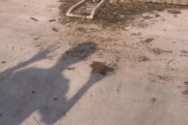
(a) ${\bm{f}}$ on $\Omega$

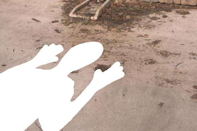
(b) ${\bm{f}}$ on $\Omega_{\text{out}}$

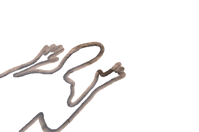
(c) ${\bm{f}}$ on $\Omega_{\text{sb}}$

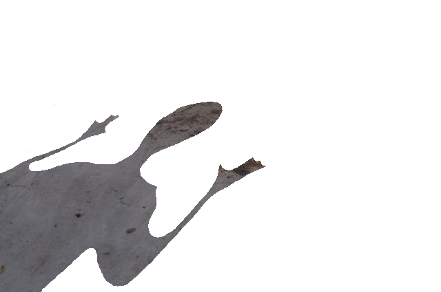
(d) ${\bm{f}}$ on $\Omega_{\text{in}}$

Figure 1: Decomposition of $\Omega$ as in (3) into (b) unshadowed region, (c) shadow boundaries and (d) shadowed region for a discrete shadowed image ${\bm{f}}$.

Provided that a decomposition as in (3) is given, which for real images may a challenging problem on its own regard [8], the osmosis model (2) can be easily adapted to solve the shadow removal problem by simply defining the vector field ${\bm{d}}$ in (2) in terms of a shadowed image $f$ as ${\bm{d}}:={\bm{\nabla}}\log f$ on $\Omega_{\text{in}}\cup\Omega_{\text{out}}$ and ${\bm{d}}=0$ on $\Omega_{\text{sb}}$. The continuous osmosis model adapted to shadow removal then reads

$$\begin{cases}u_{t}=\mathrm{\Delta}u-\mathrm{div}({\bm{d}}u)&\text{on }\Omega_{\text{in}}\cup\Omega_{\text{out}}\times(0,T],\\ u_{t}=\mathrm{\Delta}u&\text{on }\Omega_{\text{sb}}\times(0,T],\\ u({\bm{x}},0)=f({\bm{x}})&\text{on }\Omega,\\ \langle\,{\bm{\nabla}}u-{\bm{d}}u,{\bm{n}}\,\rangle=0&\text{on }\partial\Omega\times(0,T].\end{cases}$$ (4)

The evolution on the shadow boundary $\Omega_{\text{sb}}$ can be interpreted as an inpainting step where information is propagated from $\Omega_{\text{out}}$ to $\Omega_{\text{in}}$ over $\Omega_{\text{sb}}$. Due to the action of the Laplace operator on $\Omega_{\text{sb}}$, image structures in $\Omega_{\text{in}}\cup\Omega_{\text{out}}$ are isotropically diffused on $\Omega_{\text{sb}}$, resulting in a shadowless, but blurred inpainting result on $\Omega_{\text{sb}}$. To overcome this a post-processing inpainting step is commonly applied, as for instance in Figure 2.

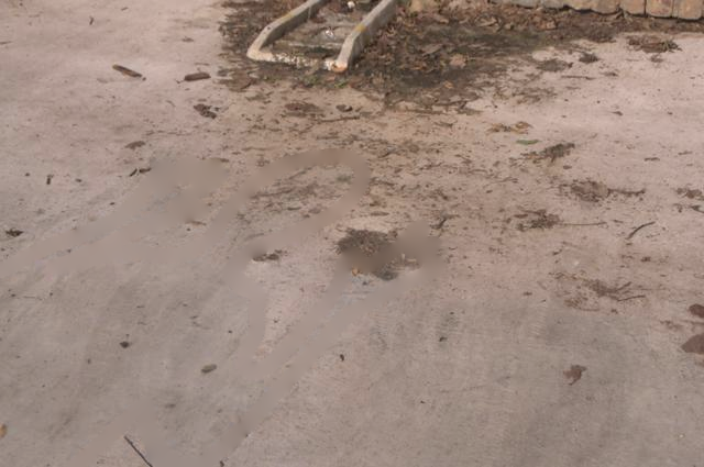
(a) Isotropic osmosis [38]

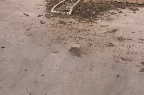
(b) Post-processing inpainting step [2]

(c) Zoom of Figure 2(a) (top) and 2(b) (bottom)

Figure 2: Shadow removal for Figure 1(a) via (4) in Figure 2(a) and with post-processing inpainting correction in Figure 2(b) to remove the blurring artefacts due to Laplace inpainting on $\Omega_{\text{sb}}$ in (4).

Note that in natural images several acquisition and/or compression artefacts may render the automatic segmentation of the shadow boundary very challenging. On the other hand, its accurate manual selection may be very tedious. In many practical examples, a rough selection of $\Omega_{\text{sb}}$ is therefore performed manually by using a brush whose possibly large thickness may badly affect the result of the model (4) (see Figure 4) due to the Laplace blurring artefacts discussed above.

Vogel et al.  [36] have presented a discrete osmosis theory and have proven that explicit and implicit finite difference discretisations satisfy its requirements. Different splitting schemes have been considered in [5, 27] and have been applied to imagery for cultural heritage conservation.

1.3 Scope of the paper

In this paper we extend the isotropic osmosis model (2) and its shadow removal application (4) to a model that features anisotropic diffusion in the flavour of (1) and adapts concepts from anisotropic diffusion inpainting [39, 13]. This will be implemented by incorporating local directionality depending on image orientations. We show that with this modification we can improve the solution of the shadow removal problem, in particular overcoming blurring artefacts in the region around the shadow boundary, without additional post-processing steps. In the integrable case, the resulting drift-diffusion PDE can be derived as the gradient flow of a suitable energy depending on local gradient information. To estimate such local directionality, we adapt the tensor voting framework proposed in [16]. For the numerical solution we combine a numerical time-stepping method based on exponential integrator techniques with the nonnegative space discretisation of Fehrenbach and Mirebeau [10]. Our model is validated on several synthetic and natural images affected by constant shadows. Results show good light-balance properties and, compared to plain isotropic osmosis models, avoid the smoothing artefacts on the shadow boundary. An illustrative example of the performance of our model is reported in Figure 3.

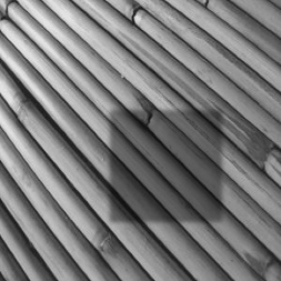
(a) Shadowed image

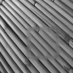
(b) Isotropic osmosis [38]

(c) Proposed solution

Figure 3: Comparison of solutions obtained by solving the isotropic model considered in [38, 36] and our anisotropic one to solve the shadow removal problem.

Organisation of the paper.

In Section 2 we introduce the anisotropic osmosis model and study analytically its properties. Then, in Section 3 we study space and time discretisation schemes for the anisotropic model. Finally, in Section 4 we show the application of the anisotropic model to solve the shadow removal problem.

2 Anisotropic osmosis

We present in this section a variation of the classical osmosis model (2) encoding local directional information of the image in the diffusion term, propagating geometric structures dominantly along locally preferred directions. For this reason we call our model anisotropic osmosis model in contrast to the model (2) which we refer to as isotropic osmosis model.

In what follows we introduce the general form of our anisotropic osmosis model and state some properties of solutions that are inherited from the isotropic model. For specific choices of anisotropy we also show connections of the anisotropic osmosis model to anisotropic diffusion-based inpainting methods such as edge-enhancing anisotropic diffusion [39]. Out of these specific instances we derive our proposed anisotropic osmosis-inpainting model for shadow removal.

2.1 Definitions and modelling

Let us define an anisotropic osmosis energy as follows.

Definition 2.1 (Anisotropic osmosis energy).

Let $\Omega\subset\mathbb{R}^{2}$, $u,v\in H^{1}(\Omega;\mathbb{R}_{+})$ be two positive images and let $\mathbf{W}:\Omega\to\mathbb{R}^{2}$ be a positive semi-definite symmetric matrix field. We define the anisotropic osmosis energy of $u$ with respect to $\mathbf{W}$ and the reference image $v$ as

$$E(u)=\int_{\Omega}v({\bm{x}})\,{\bm{\nabla}}^{\top}\!\left(\frac{u({\bm{x}})}{v({\bm{x}})}\right)\mathbf{W}({\bm{x}})\,{\bm{\nabla}}\left(\frac{u({\bm{x}})}{v({\bm{x}})}\right)\mathop{}\!\mathrm{d}{\bm{x}}.$$ (5)

We will also use the following alternative notation for $E$:

$$E(u)=\int_{\Omega}v({\bm{x}})\;\left\|{\bm{\nabla}}\left(\frac{u({\bm{x}})}{v({\bm{x}})}\right)\right\|^{2}_{\mathbf{W}}\mathop{}\!\mathrm{d}{\bm{x}}$$ (6)

where $\|{\bm{e}}\|_{\mathbf{W}}:=\sqrt{\langle{\bm{e}},\,\mathbf{W}{\bm{e}}\rangle}$.

Remark 2.2 (Isotropic case).

If $\mathbf{W}$ is the identity matrix, then (5) corresponds to the isotropic osmosis energy considered in [38].

Next we define an anisotropic osmosis evolution whose steady state minimises our anisotropic osmosis energy.

Proposition 2.3.

Let $v:\Omega\to\mathbb{R}_{+}$ be a positive image, ${\bm{d}}\in\mathbb{R}^{2}$ the vector field defined as ${\bm{d}}:={\bm{\nabla}}\log v$ and $\mathbf{W}:\Omega\to\mathbb{R}^{2}$ be a positive semi-definite symmetric matrix field. Then, for a given positive image $f\in L^{\infty}(\Omega;\mathbb{R}_{+})$ the solution of the Euler-Lagrange equation of the functional $E$ defined in (2.1) is the steady state of the anisotropic image osmosis model

$$\begin{cases}u_{t}=\mathrm{div}\left(\mathbf{W}({\bm{\nabla}}u-{\bm{d}}u)\right)&\text{on }\Omega\times(0,T],\\ u({\bm{x}},0)=f({\bm{x}})&\text{on }\Omega,\\ \langle\,\mathbf{W}\left({\bm{\nabla}}u-{\bm{d}}u\right),{\bm{n}}\,\rangle=0&\text{on }\partial\Omega\times(0,T].\end{cases}$$ (7)

Proof.

For any test function $\varphi\in C^{\infty}_{c}(\Omega)$, we compute the optimality condition holding for any critical point $u$ of $E$. We get:

$$\frac{\partial u}{\partial\tau}\left(E(u+\tau\varphi)\right)_{|\tau=0} =2\int_{\Omega}v~{}\left\langle\mathbf{W}{\bm{\nabla}}\left(\frac{u}{v}\right),{\bm{\nabla}}\left(\frac{\varphi}{v}\right)\right\rangle\mathop{}\!\mathrm{d}{\bm{x}}$$

$$=-2\int_{\Omega}\mathrm{div}\left(v\mathbf{W}{\bm{\nabla}}\left(\frac{u}{v}\right)\right)\frac{\varphi}{v}\mathop{}\!\mathrm{d}{\bm{x}}$$

$$=-2\int_{\Omega}\frac{1}{v}\mathrm{div}\left(v\mathbf{W}\left(\frac{{\bm{\nabla}}u}{v}-\frac{u{\bm{\nabla}}v}{v^{2}}\right)\right)\varphi\mathop{}\!\mathrm{d}{\bm{x}}=0,$$

where we have applied the divergence theorem and the Neumann boundary conditions in (7). Due to the positivity of $v$ and since $\varphi$ is compactly supported in $\Omega$, we have that for any ${\bm{x}}\in\Omega$:

$$0=\mathrm{div}\left(v\mathbf{W}\left(\frac{{\bm{\nabla}}u}{v}-\frac{u{\bm{\nabla}}v}{v^{2}}\right)\right)=\mathrm{div}\left(\mathbf{W}\left({\bm{\nabla}}u-\frac{{\bm{\nabla}}v}{v}u\right)\right)$$

By definition of ${\bm{d}}=\frac{{\bm{\nabla}}v}{v}$, we note that the above corresponds to the following PDE:

$$\mathrm{div}\left(\mathbf{W}\left({\bm{\nabla}}u-{\bm{d}}u\right)\right)=0,$$

which is the steady state of (7). ∎

Similar to the isotropic osmosis PDE (2), the anisotropic model (7) enjoys some properties which makes it amenable for imaging applications.

Theorem 2.4.

The solution $u:\Omega\to\mathbb{R}$ of the anisotropic osmosis model (7) satisfies the following properties:

1. conservation of the average grey value:

   $$\frac{1}{|\Omega|}\int_{\Omega}u({\bm{x}},t)\mathop{}\!\mathrm{d}{\bm{x}}=\frac{1}{|\Omega|}\int_{\Omega}f({\bm{x}})\mathop{}\!\mathrm{d}{\bm{x}},\quad\text{for all }t>0;$$

2. preservation of non-negativity:

   $$u({\bm{x}},t)\geq 0,\quad\text{for all }{\bm{x}}\in\Omega\quad\text{and}\quad t>0;$$

3. non-constant steady states: The steady state of (7) is given by

   $$w({\bm{x}}):=\frac{\mu_{f}}{\mu_{v}}v({\bm{x}}).$$ (8)

Proof.

We follow [38] and prove statements (i)–(iii) in turn.

1. Let $\mu_{u}(t):=\frac{1}{|\Omega|}\int_{\Omega}u({\bm{x}},t)\mathop{}\!\mathrm{d}{\bm{x}}$ be the average grey value of the image $u$ at time $t\geq 0$. Applying the divergence theorem and the homogeneous Neumann boundary conditions in (7) we obtain:

   $$\frac{d\mu_{u}}{dt}=\frac{1}{|\Omega|}\int_{\Omega}u_{t}\mathop{}\!\mathrm{d}{\bm{x}} =\frac{1}{|\Omega|}\int_{\Omega}\mathrm{div}\left(\mathbf{W}\left({\bm{\nabla}}u-{\bm{d}}u\right)\right)\mathop{}\!\mathrm{d}{\bm{x}}$$

   $$=\int_{\partial\Omega}\langle\,\mathbf{W}\left({\bm{\nabla}}u-{\bm{d}}u\right),{\bm{n}}\,\rangle\mathop{}\!\mathrm{d}S=0,$$

   and the statement follows.

2. Assume that $T>0$ is the smallest time such that $\min_{{\bm{x}},t}u({\bm{x}},t)=0$, and that this minimum is attained in some inner point $\bm{\mu}\in\Omega$. Since we have ${\bm{\nabla}}u(\bm{\mu},T)=u(\bm{\mu},T)=0$, we deduce:

   $$u_{t}(\bm{\mu},T)= \mathrm{div}\left(\mathbf{W}{\bm{\nabla}}u(\bm{\mu},T)\right)-\mathrm{div}\left(\mathbf{W}{\bm{d}}u(\bm{\mu},T)\right)$$ (9)

   $$= \mathbf{W}\cdot\mathrm{D}^{2}u(\bm{\mu},T)+\left(\mathrm{div}(\mathbf{W})-\mathbf{W}{\bm{d}}\right)\cdot\underbrace{{\bm{\nabla}}u(\bm{\mu},T)}_{=0}-\mathrm{div}(\mathbf{W}{\bm{d}})\underbrace{u(\bm{\mu},T)}_{=0}$$

   $$= \mathbf{W}\cdot\mathrm{D}^{2}u(\bm{\mu},T),$$

   that is in correspondence to the point $(\bm{\mu},T)$, the anisotropic osmosis equation behaves like the diffusion equation

   $$u_{t}=\mathbf{W}\cdot\mathrm{D}^{2}u,$$ (10)

   with non-constant positive semidefinite diffusivity matrix $\mathbf{W}$. For such equations a generalisation of the weak minimum/maximum principle (which holds in its classical form only for positive definite, i.e. elliptic, operators) holds true, see, e.g.  [30]. Therefore, for any $t\geq T$ the solution of the anisotropic model remains non-negative and since the solution has been further assumed to be strictly positive for all $t<T$, including $t=0$ due to the positivity of $f$, we have that it stays actually non-negative for any $t\geq 0$.

3. For any $c\in\mathbb{R}$, the function $w:=cv$ endowed with the Neumann-type boundary conditions in (7) solves the steady state equation of the system anisotropic PDE, since there trivially holds:

   $$\mathrm{div}\left(\mathbf{W}\left({\bm{\nabla}}w-\frac{{\bm{\nabla}}v}{v}w\right)\right)=\mathrm{div}\left(\mathbf{W}\left(c{\bm{\nabla}}v-\frac{{\bm{\nabla}}v}{v}cv\right)\right)=0.$$

   Due to mass and non-negativity conservation, the process is then forced to a non-negative steady state solution $w$ of such a form. Furthermore, the constant $c\in\mathbb{R}$ can be easily found by noticing

   $$c\mu_{v}=\frac{1}{|\Omega|}\int_{\Omega}cv({\bm{x}})\mathop{}\!\mathrm{d}{\bm{x}}=\frac{1}{|\Omega|}\int_{\Omega}w({\bm{x}})\mathop{}\!\mathrm{d}{\bm{x}}=\frac{1}{|\Omega|}\int_{\Omega}f({\bm{x}})\mathop{}\!\mathrm{d}{\bm{x}}=\mu_{f},$$

   whence $c=\mu_{f}/\mu_{v}$ which is well defined since $v$ is strictly positive in $\Omega$.∎

2.2 Anisotropic diffusion inpainting

Anisotropic diffusion inpainting with a diffusion tensor has been introduced in [39] and applied successfully for inpainting-based compression [13, 33]. It exploits the edge-enhancing anisotropic diffusion filter that has been proposed for image denoising [37]. In order to propagate structures from specified image regions into inpainting regions, one uses the differential operator $\mathrm{div}(\mathbf{D}({\bm{\nabla}}u_{\sigma}){\bm{\nabla}}u)$, where $u_{\sigma}$ denotes the convolution of $u$ with a Gaussian of standard deviation $\sigma$. The diffusion tensor $\mathbf{D}$ has eigenvectors perpendicular and parallel to ${\bm{\nabla}}u_{\sigma}$. Its corresponding eigenvalues are given by

$$\mu_{1}(|{\bm{\nabla}}u_{\sigma}|)=1\quad\text{and}\quad\mu_{2}(|{\bm{\nabla}}u_{\sigma}|)=\frac{1}{\sqrt{1+|{\bm{\nabla}}u_{\sigma}|^{2}/\lambda^{2}}},$$ (11)

with some contrast parameter $\lambda>0$. Thus, the goal is to inpaint fully in the direction of an oriented structure, and to reduce the inpainting perpendicular to a structures, if its contrast is large. Processes of this type can inpaint edge-like structures even when the specified data are sparse and the gaps to be bridged are large [33]. However, they are not well-suited to shadow removal problems, since the shadow boundaries create unphysical edges. Therefore, we will have to modify these ideas such that the local structure directions become more robust w.r.t.  shadow boundaries. To this end, we will consider and modify more refined structure descriptors such as tensor voting. This will be done next.

2.3 Computation of structure directions via tensor voting

In this section we present a work-flow which is locally insensitive to the light jump produced by the shadow. This will serve us to force anisotropy on $\Omega_{\text{sb}}$ along suitable directions.

A standard way to provide an estimate of the local structure orientation in an image $u$ consists in computing the eigenvector ${\bm{e}}_{1}$ associated to the leading eigenvalue $\lambda_{1}$ of the structure tensor $\mathbf{J}_{\rho}(u)$ [37] associated to $u$. By fixing $\sigma,\rho>0$ to be the pre- and post-smoothing parameters, we recall that the structure tensor $\mathbf{J}_{\rho}(u)$ of an image $u$ is defined as:

$$\mathbf{J}_{\rho}(u):=K_{\rho}\ast\mathbf{J}_{0}(u),\quad\text{with}\quad\mathbf{J}_{0}(u):={\bm{\nabla}}u_{\sigma}\otimes{\bm{\nabla}}u_{\sigma},$$

where $u_{\sigma}:=K_{\sigma}\ast u$ is a smoothed version of the image $u$ and $K_{\sigma},K_{\rho}$ are Gaussian convolution kernels. Usually, $\sigma$ and $\rho$ are chosen so that $\sigma\ll\rho$, where $\sigma$ is associated to the noise scale and $\rho$ integrates the orientation information. Denoting by $\lambda_{1}\geq\lambda_{2}$ the eigenvalues of $\mathbf{J}_{\rho}(u)$ and by ${\bm{e}}_{1},{\bm{e}}_{2}$ the associated eigenvectors, a classification of the different structural image information in terms of the size of $\lambda_{1}$ and $\lambda_{2}$ can be made following, e.g., [18, 11, 20]. For any ${\bm{x}}\in\Omega$ we thus have:

• If $\lambda_{1}({\bm{x}})\approx\lambda_{2}({\bm{x}})\approx 0$, then ${\bm{x}}$ is likely to belong to a homogeneous region;

• If $\lambda_{1}({\bm{x}})\gg\lambda_{2}({\bm{x}})\approx 0$, then ${\bm{x}}$ is likely to lie on an edge;

• If $\lambda_{1}({\bm{x}})\approx\lambda_{2}({\bm{x}})\gg 0$, then ${\bm{x}}$ is likely to be a corner point.

Tensor Voting has been originally introduced in [16] for extracting curves in noisy images by means of the grouping of local features consistent in a neighbourhood of the measurements. Such framework improves the robustness of structure tensor estimation in presence of noise and image artefacts [24]. Assuming that a generic 2-tensor $\mathbf{B}$ in $\mathbb{R}^{2}$ has the following matrix representation:

$$\mathbf{B}=\begin{pmatrix}b_{11}&b_{12}\\ b_{21}&b_{22}\end{pmatrix}=\lambda_{1}({\bm{e}}_{1}\otimes{\bm{e}}_{1})+\lambda_{2}({\bm{e}}_{2}\otimes{\bm{e}}_{2})$$ (12)

where $\lambda_{1},\lambda_{2}$ are the eigenvalues associated to the eigenvectors ${\bm{e}}_{1}$ and ${\bm{e}}_{2}$, respectively, we have that (12) can be equivalently rewritten as

$$\mathbf{B}=(\lambda_{1}-\lambda_{2})({\bm{e}}_{1}\otimes{\bm{e}}_{1})+\lambda_{2}({\bm{e}}_{1}\otimes{\bm{e}}_{1}+{\bm{e}}_{2}\otimes{\bm{e}}_{2}).$$

We can now distinguish the two following quantities:

• $(\lambda_{1}-\lambda_{2})$ is called saliency or stickness. It provides an estimation of the confidence on the direction ${\bm{e}}_{1}$ and it is also called orientation certainty or anisotropy measure;

• $\lambda_{2}$ is called ballness and it measures the size of the minor-axis of the anisotropy ellipse. Since it is in some sense a measure of how the estimation of the main estimated direction is contradicted, it is often called orientation uncertainty or junctionness.

The tensor voting operation consists in adding, at each iteration, the contribution of neighbourhood tensors for each point in the domain, resulting in an enhanced tensor field due to the presence of saliency parameter. In [12] the authors show that the complexity of the original approach may be time-consuming, even for small images. Thus, they propose an efficient computation of the tensor voting framework based on steerable filters theory, i.e. complex-valued convolutions.

For the shadow removal application we are considering, the estimation of the structure direction ${\bm{e}}_{1}$ may be affected by the shadow edges, which do not correspond to the actual underlying image structures. The presence of such edges make the use of either the structure tensor or the tensor voting very challenging for estimating the local directions.

To circumvent this problem, we propose a modification of the tensor voting framework by means of interpreting shadow edges as bias in the estimation of the structure. From the given initial blurred image $u_{\sigma}$, we firstly compute the local orientation $\theta$ of the gradient from the eigenvector ${\bm{e}}_{2}$. Secondly, we compute the saliency of the given shadowed image. Finally we apply the tensor voting framework with a modified saliency and orientation on $\Omega_{\text{sb}}$ so as to mark the shadow boundaries as bias: there, the saliency is zeroed and the orientation is initialised at random. Details on the algorithm and results are presented in Section 4.2.1.

2.4 An anisotropic osmosis-inpainting model for shadow removal

Let $f:\Omega\to\mathbb{R}_{+}$ be a positive greyscale image with a constant shadow and let $\Omega$ be decomposed as in (3). We propose the following structure-preserving osmosis model for solving the shadow removal problem:

$$\begin{dcases}u_{t}=\mathrm{div}\left(\mathbf{W}({\bm{\nabla}}u-{\bm{d}}u\right))&\text{on }\Omega\times(0,T],\\ u({\bm{x}},0)=f({\bm{x}})&\text{on }\Omega,\\ \langle\,\mathbf{W}\left({\bm{\nabla}}u-{\bm{d}}u\right),{\bm{n}}\,\rangle=0&\text{on }\partial\Omega\times(0,T],\end{dcases}$$ (13)

Here we define the discontinuous vector field ${\bm{d}}$ and the discontinuous matrix field $\mathbf{W}$ as

$${\bm{d}}({\bm{x}}) = \begin{dcases}{\bm{\nabla}}\log f,&\text{if }{\bm{x}}\in\Omega\setminus\Omega_{\text{sb}},\\ 0,&\text{if }{\bm{x}}\in\Omega_{\text{sb}},\end{dcases}$$ (14)

$$\mathbf{W}({\bm{x}}) = \begin{dcases}\mathbf{I},\quad&\text{if }{\bm{x}}\in\Omega\setminus\Omega_{\text{sb}},\\ \epsilon({\bm{e}}_{1}\otimes{\bm{e}}_{1})+1({\bm{e}}_{2}\otimes{\bm{e}}_{2}),\quad&\text{if }{\bm{x}}\in\Omega_{\text{sb}}.\end{dcases}$$ (15)

where $\mathbf{I}$ denotes the $2\times 2$ identity matrix, and ${\bm{e}}_{1}$ and ${\bm{e}}_{2}$ are the directions from our modified tensor voting applied to the initial image $f$.

This means, an isotropic osmosis evolution is performed in $\Omega_{\text{sb}}^{c}$, while an anisotropic inpainting is performed on $\Omega_{\text{sb}}$. In other words, classical osmosis balances image intensity in the shadowed region with respect to the unshadowed regions, while the nonlinear interpolation preserves structures and avoids blurring on the shadow boundary. The proposed model performs the osmosis and the inpainting step jointly and avoids any post-processing step.

3 Space and time discretisation

We now discuss appropriate discretisations of the anisotropic osmosis model that are consistent with the continuous model (7) and preserve some of its properties as stated in Theorem 2.4. To do so, we consider a discrete rectangular image domain with $M\times N$ pixels. Let $S:=MN$. The given positive initial image ${\bm{f}}$ is then defined as a vector in $\mathbb{R}^{S}_{+}$. For a given grid step size $h>0$, we denote by ${\bm{u}}=(u_{i,j})_{i,j}$ the approximation of the function $u$ and with $u_{i,j}$ its approximated value in suitable discretisation nodes $((i-\frac{1}{2})h,(j-\frac{1}{2})h)$ with $i=1,\ldots,M$ and $j=1,\ldots,N$. Similarly, for $k\geq 0$ we denote by $u^{k}_{i,j}$ the value of $u_{i,j}$ at the time node $t_{k}=k\tau$, where $\tau$ is the time step size. Also, for ${\bm{x}}\in\Omega$, we denote by $\bm{\lambda}_{1},\bm{\lambda}_{2}\in\mathbb{R}_{+}^{S}$ the discretised eigenvalues $\lambda_{1}({\bm{x}})$ and $\lambda_{2}({\bm{x}})$, while by $\bm{\theta}\in[0,2\pi)^{S}$ the discretised orientation $\theta({\bm{x}})$.

3.1 Discrete osmosis theory

A discrete theory for osmosis models has been established in [36]. Since it is also applicable to the anisotropic setting, we report here the general result [36, Proposition 1] and list in the following some discrete solvers fulfilling its assumptions.

Theorem 3.1 ([36]).

For a given ${\bm{f}}\in\mathbb{R}^{S}_{+}$, consider the fully-discretised problem:

$${\bm{u}}^{0}={\bm{f}},\qquad{\bm{u}}^{k+1}=\mathbf{P}{\bm{u}}^{k},\qquad k\geq 1,$$ (16)

where the (unsymmetric) matrix $\mathbf{P}\in\mathbb{R}^{S\times S}$ is an irreducible, non-negative matrix with strictly positive diagonal entries and unitary column sum . Then the following properties hold true:

1. The evolution preserves positivity and the average grey value of ${\bm{f}}$;

2. The eigenvector of $\mathbf{P}$ associated to eigenvalue $1$ is the unique steady state for $k\to\infty$.

As shown in [36] for the isotropic osmosis model, standard explicit and implicit time finite difference schemes fit this framework, the former being subject to time step size restrictions, the latter being unconditionally stable. Furthermore, both schemes converge to the space discretisation of the elliptic steady state for every stable time step size. For the implicit scheme with a BiCGStab solver, Vogel et al. [36] report speed-ups of two orders of magnitude compared to the explicit method. In [5] a Peaceman-Rachford splitting is shown to satisfy Theorem 3.1 under a time step size restriction, while the additive operator splitting (AOS) considered in [27] fulfils Theorem 3.1 for all time step sizes. Splitting schemes such as the AOS method, however, do not converge to the space-discrete elliptic steady state solution unless the time step size goes to zero. In practice, keeping this time splitting error under control imposes bounds on the time step size.

Note that in contrast to the theory for fully discrete diffusion filters [37], the discrete osmosis theory in Theorem 3.1 does not require a symmetric matrix. Since it does also not involve any isotropy assumption, it is basically also applicable to anisotropic osmosis processes, if suitable space discretisations are employed. This, however, is not straightforward and will be discussed in the sequel.

3.2 Space discretisation with the AD-LBR stencil

In what follows, we describe the discretisation of the weighting matrix $\mathbf{W}$ and the differential operators $\mathrm{div}$ and ${\bm{\nabla}}$ for a grey-scale image of height $M$ and width $N$ unrolled as ${\bm{u}}\in\mathbb{R}^{S}$, with $S=MN$, that defines the spatial discretisation matrix $\mathbf{A}$ for the semi-discrete osmosis problem

$$\begin{dcases}{\bm{u}}^{\prime}(t)=\mathbf{A}{\bm{u}}(t),&\text{for }t\in(0,T],\\ {\bm{u}}(0)={\bm{f}},\end{dcases}$$ (17)

where $T>0$ is a positive final time.

While diffusion processes are stable in many aspects, e.g. in terms of decreasing $L^{2}$ norms and decreasing $L^{\infty}$ norms, the stability of osmosis processes is restricted to essentially one key property: the preservation of nonnegativity. Thus, any suitable space discretisation for osmosis filters should guarantee that it is nonnegativity preserving. For the matrix $\mathbf{A}$ this implies that all off-diagonal elements must be nonnegative. While this is easily satisfied for standard discretisations of isotropic processes [36], it becomes much more challenging for anisotropic approaches: The drift term is fairly unproblematic and can be handled e.g. with classical upwind discretisations. However, most discretisations of the diffusion term $\mathrm{div}(\mathbf{W}{\bm{\nabla}}u)$ are only stable in the $L^{2}$ norm [40]. Thus, they cannot guarantee preservation of nonnegativity. Nonnegativity-preserving discretisations can be found in [37, 25, 10]. In our paper, we use the stencil of Fehrenbach and Mirebeau [10], since it is a fairly sophisticated nonnegativity-preserving method that has been reported to give good results. This anisotropic diffusion discretisation relies on lattice basis reduction ideas and is called AD-LBR. Let us sketch its underlying ideas.

In [10], the authors tackle the minimisation of an anisotropic energy which in our notation reads:

$$E(u)=\int_{\Omega}\|{\bm{\nabla}}u({\bm{x}})\|_{\mathbf{W}}^{2}\mathop{}\!\mathrm{d}{\bm{x}},$$

where $\|{\bm{e}}\|_{\mathbf{W}}:=\sqrt{\langle{\bm{e}},\,\mathbf{W}{\bm{e}}\rangle}$, for any ${\bm{e}}\in\mathbb{R}^{d}$ and $\mathbf{W}$ is symmetric and positive definite. The idea is to introduce a discretisation $E_{h}$ of the energy above on the discretised domain $\Omega_{h},h>0$ via a sum of weighted squared differences of $u\in L^{2}(\Omega_{h};\mathbb{R})$, i.e.:

$$E_{h}(u)=h^{d-2}\sum_{{\bm{x}}\in\Omega_{h}}\sum_{{\bm{e}}\in V({\bm{x}})}\gamma_{x}({\bm{e}})|u({\bm{x}}+h{\bm{e}})-u({\bm{x}})|^{2},$$ (18)

where $V({\bm{x}})\subset\mathbb{Z}^{d}$ is the stencil and $\gamma_{\bm{x}}({\bm{e}})\geq 0$ are the associated weights. The key step is the linearisation of $u({\bm{x}}+h{\bm{e}})$ as $u({\bm{x}})+\langle{\bm{\nabla}}u({\bm{x}}),\,h{\bm{e}}\rangle$, which shows that for each ${\bm{x}}\in\Omega_{h}$ and smooth $u$ one can write:

$$h^{d}\|{\bm{\nabla}}u\|_{\mathbf{W}}^{2}=h^{d-2}\sum_{{\bm{e}}\in V({\bm{x}})}\gamma_{\bm{x}}({\bm{e}})\langle{\bm{\nabla}}u({\bm{x}}),h{\bm{e}}\rangle^{2},$$

which turns out to be equivalent to require the condition $\mathbf{W}=\sum_{{\bm{e}}\in V({\bm{x}})}\gamma_{\bm{x}}({\bm{e}}){\bm{e}}{\bm{e}}^{\mathrm{T}}$. via the following Lemma [10, Lemma 1].

Lemma 3.2.

Let ${\bm{e}}_{0},{\bm{e}}_{1},{\bm{e}}_{2}\in\mathbb{R}^{2}$ be such that ${\bm{e}}_{0}+{\bm{e}}_{1}+{\bm{e}}_{2}=0$ and $|\mathrm{det}({\bm{e}}_{1},{\bm{e}}_{2})|=1$. Then for any symmetric positive definite matrix $\mathbf{W}$, there holds:

$$\mathbf{W}=-\sum_{0\leq i\leq 2}\langle{\bm{e}}_{i+1}^{\perp},\,\mathbf{W}{\bm{e}}_{i+2}\rangle{\bm{e}}_{i}{\bm{e}}_{i}^{\mathrm{T}},$$

under the convention ${\bm{e}}_{3+i}:={\bm{e}}_{i}$

Actually, for any dimension $d\leq 3$ and any symmetric positive definite $d\times d$ matrix $\mathbf{M}$, there always exists a family $({\bm{e}}_{i})_{i\in I}$ of vectors in $\mathbb{R}^{d}$ such that $\langle{\bm{e}}_{i},\mathbf{M}{\bm{e}}_{j}\rangle\leq 0$ for any $i\neq j$. Such a family is called $\mathbf{M}$-obtuse [9]. Thus, by taking $({\bm{e}}_{0},{\bm{e}}_{1},{\bm{e}}_{2})$ as a $\mathbf{W}$-obtuse superbase of $\mathbb{Z}^{2}$ (i.e. a basis of $\mathbb{Z}^{2}$ with $|\mathrm{det}({\bm{e}}_{0},{\bm{e}}_{1},{\bm{e}}_{2})|=1$ such that ${\bm{e}}_{0}+{\bm{e}}_{1}+{\bm{e}}_{2}=0$), a stencil $V({\bm{x}}):=\{{\bm{e}}_{0},{\bm{e}}_{1},{\bm{e}}_{2},-{\bm{e}}_{0},-{\bm{e}}_{1},{\bm{e}}_{2}\}$ can be used to write explicitly the coefficients $\gamma_{\bm{x}}$ in (18) for $0\leq i\leq 2$ as done in [10, Equation (11)]:

$$\gamma_{\bm{x}}(\pm{\bm{e}}_{i}):=-\frac{1}{2}\langle{\bm{e}}_{i+1}^{\perp},\,\mathbf{W}{\bm{e}}_{i+2}^{\perp}\rangle.$$

The resulting stencil is shown to be independent of the choice of the superbase [10, Lemma 11] and it is orientated along the preferred diffusion direction given by $\mathbf{W}$. Also, the AD-LBR scheme is sparse, i.e. it has a limited support of 6 points for two-dimensional images.

In the AD-LBR discretisation, an important role is played by the anisotropic ratio $\kappa\in[1,\infty)$, which measures the geometrical shape of the ellipse associated to the eigen-decomposition of the anisotropic matrix $\mathbf{W}$: the closer $\kappa$ is to 1, the more $\mathbf{W}$ is similar to the identity matrix $\mathbf{I}$. The computation of the stencil has a logarithmic cost in the anisotropy ratio $\kappa$ of the diffusion tensor, making AD-LBR appealing for applications. Also, by fixing a direction $\theta$ all over the domain $\Omega$ for $\mathbf{W}$, the anisotropy ratio $\kappa$ can be related to the eigenvalues of $\mathbf{W}$; see [10, Equation 60]. For instance, if $\mathbf{W}$ has eigenvalues $\varepsilon$ and $1$ with $0<\varepsilon\ll 1$, then $\varepsilon=1/\kappa^{2}$. For completeness, we report in Table 1 the AD-LBR stencil for different choices of $\varepsilon$ and a fixed angle $\theta=2\pi/3$ that characterises the second eigenvector ${\bm{e}}_{2}=(\cos\theta,\sin\theta)^{\top}$ of $\mathbf{W}$; cf. also [10, Table 1,Table 2].

Table 1: AD-LBR stencil for the discretisation of $\mathrm{div}(\mathbf{W}{\bm{\nabla}}(\,{\cdot}\,))$: Different choices of $\varepsilon$ are presented with fixed angle $\theta=2\pi/3$ for the first eigenvector. In bold we denote the $(i,j)$ entry. As expected, we observe that in the case of strong anisotropy, the stencil becomes aligned in $\theta$ direction.

$\varepsilon=1$ ($\kappa=1$, $\mathbf{W}=\mathbf{I}$)	$\varepsilon=0.5$ ($\kappa=\sqrt{2}$)	$\varepsilon=0.1$ ($\kappa=\sqrt{10}$)	$\varepsilon=0.02$ ($\kappa=\sqrt{50}$)
$\displaystyle 0.00$ $\displaystyle 1.00$ $\displaystyle 0.00$ $\displaystyle 1.00$ $\displaystyle\mathbf{-4.00}$ $\displaystyle 1.00$ $\displaystyle 0.00$ $\displaystyle 1.00$ $\displaystyle 0.00$	$\displaystyle 0.00$ $\displaystyle 0.41$ $\displaystyle 0.22$ $\displaystyle 0.66$ $\displaystyle\mathbf{-2.57}$ $\displaystyle 0.66$ $\displaystyle 0.22$ $\displaystyle 0.41$ $\displaystyle 0.00$	$\displaystyle 0.00$ $\displaystyle 0.26$ $\displaystyle 0.26$ $\displaystyle 0.26$ $\displaystyle\mathbf{-1.16}$ $\displaystyle 0.26$ $\displaystyle 0.26$ $\displaystyle 0.26$ $\displaystyle 0.00$	$\displaystyle 0.00$ $\displaystyle 0.11$ $\displaystyle 0.16$ $\displaystyle 0.01$ $\displaystyle\mathbf{-0.55}$ $\displaystyle 0.01$ $\displaystyle 0.16$ $\displaystyle 0.11$ $\displaystyle 0.00$

Remark 3.3.

By construction, the AD-LBR space discretisation matrix $\mathbf{A}$ has 0 column sum and non-negative off-diagonal entries. Moreover, our numerical experiments give strong evidence that $\mathbf{A}$ is also irreducible. However, a formal proof of the irreducibility of $\mathbf{A}$ is left for future research.

3.3 Exact time discretisation

In this section we see how it is possible to solve the dynamical system (17), through a highly accurate approximation of the exact solution

$${\bm{u}}(T)=\exp(T\mathbf{A}){\bm{f}}.$$ (19)

First of all, we notice that it is not necessary to compute the large and dense matrix $\exp(T\mathbf{A})$ explicitly. It is sufficient to compute only its action on the initial solution ${\bm{f}}$. Polynomial methods (see, for instance, [31, 6, 1], approximate the action of the exponential by a polynomial of a certain degree applied to the initial vector. They do not require to solve a linear system of equations: usually they scale the matrix and approximate the solution by an iterative procedure like

$${\bm{u}}^{k+1}=p_{m_{k}}(\alpha_{k}\tau\mathbf{A}){\bm{u}}^{k},\quad k=0,1,\ldots,K-1,\quad{\bm{u}}^{0}={\bm{f}}$$

where $p_{m_{k}}$ is a polynomial of degree $m_{k}$ which approximates the exponential function and

$$\sum_{k=0}^{K-1}\alpha_{k}=1.$$

After the last iteration, ${\bm{u}}^{K}\approx{\bm{u}}(T)$. Such an iterative scheme is usually needed in order to achieve a sufficiently accurate result. For Krylov methods (like [31]), it is also necessary in order to keep the computational cost as low as possible, since the cost to produce $p_{m_{k}}$ requires $\mathcal{O}(m_{k}^{2})$ scalar products with vectors of the size of ${\bm{f}}$. Among the polynomial methods, the truncated Taylor series [1] and the interpolation in the Newton form at Leja points [6] are able to bound the relative backward error. This means that they construct an approximation in $K$ iterations with time step size $\tau=T/K$:

$${\bm{u}}^{k+1}=p_{m}(\tau\mathbf{A}){\bm{u}}^{k},\quad k=0,1,\ldots,K-1$$

such that

$$\left(p_{m}(\tau\mathbf{A})\right)^{K}{\bm{f}}=\exp(T\mathbf{A}+\delta(T\mathbf{A})){\bm{f}},\quad\text{with $\|\delta(T\mathbf{A})\|\leq\mathrm{tol}\cdot\|T\mathbf{A}\|$}.$$

The tolerance $\mathrm{tol}$ can be chosen as small as desidered. The typical value for double precision arithmetic is $2^{-53}$ and in this sense the time integration is said “exact”. The polynomial $p_{m}(z)$ is either the truncated Taylor series of $e^{z}$ about a point which depends on the spectrum of the matrix or the interpolation polynomial of $e^{z}$ at real Leja points on an interval related to the spectrum of the matrix.

The choice of the parameters $K$ and $m$ can be done by simply considering the 1-norm of $T\mathbf{A}$, or estimates of $\|(T\mathbf{A})^{q}\|_{1}^{1/q}$ for small values of $q$, or, only for interpolation at Leja points, estimates on the $\epsilon$-pseudospectra of $T\mathbf{A}$. From the implementation point of view, both algorithms simply require one matrix–vector product and one vector update at each degree elevation, and therefore the cost is $\mathcal{O}(m)$. When the spectrum of $T\mathbf{A}$ has a skinny shape, either horizontal or vertical, usually interpolation at Leja points performs better (see [6]).

Since this method can be configured to be exact in time up to machine precision, it is basically possible to reach the final time $T$ in a single time step of size $\tau=T$. However, we prefer to use multiple time steps, since the steady state $T$ is in general not known a priori. On the other hand, there is no restriction on the time step $\tau$ and it is therefore possible to implement any desired strategy for steady state detection (based, for instance, on the comparison of the solutions at two successive time steps). In particular, also variable step size $\tau_{k}$ implementations are possible without any restriction given by the stability or the computational cost.

The approximation of the action of the matrix exponential to a vector can be used also in the so called exponential integrators (we refer to the survey paper [19]) when solving general (non-linear) stiff ordinary differential equations.

3.4 Coverage through the discrete osmosis theory

A natural question in this context is whether the matrix $\mathbf{P}:=\exp(\tau\mathbf{A})$ satisfies the properties of Theorem 3.1 for suitable matrices $\mathbf{A}$. We answer this question with the following proposition, for which a simple lemma is required.

Lemma 3.4.

Let $\mathbf{C}=(c_{i,j}),\mathbf{D}=(d_{i,j})\in\mathbb{R}^{S\times S}$ be matrices with column sums $c$ and $d$, respectively. Then the matrix $\mathbf{B}:=\mathbf{C}\mathbf{D}$ has column sum $cd$.

Proof.

For every $i,j=1,\ldots,N$, we write each element $b_{i,j}$ in terms of the elements of $\mathbf{C}$ and $\mathbf{D}$. For every column $j$ we have:

$$\sum_{i=1}^{N}b_{i,j}=\sum_{i=1}^{N}\sum_{k=1}^{N}c_{i,k}d_{k,j}=\sum_{k=1}^{N}\Bigl{(}d_{k,j}\sum_{i=1}^{N}c_{i,k}\Bigr{)}=\sum_{k=1}^{N}\Bigl{(}d_{k,j}\cdot c\Bigr{)}=c\sum_{k=1}^{N}d_{k,j}=cd.\qed$$

Proposition 3.5.

Let $\mathbf{A}$ be an irreducible matrix, with column sum $0$ and non-negative off-diagonal entries. Then the (non-symmetric) matrix $\mathbf{P}:=\exp(\tau\mathbf{A})$ is an irreducible positive matrix with column sum $1$.

Proof.

We firstly show that $\mathbf{P}$ has column sum $1$. To this end, we use the expansion

$$\mathbf{P}=\exp(\tau\mathbf{A})=\sum_{k=0}^{\infty}\frac{\tau^{k}\mathbf{A}^{k}}{k!}=\mathbf{I}+\sum_{k=1}^{\infty}\frac{\tau^{k}\mathbf{A}^{k}}{k!}.$$ (20)

By hypothesis, $\mathbf{A}$ has column sum $0$. Then the column sum of $\mathbf{A}^{k}$ is $0$ for every $k\geq 1$ by Lemma 3.4. Thus, the matrix $\mathbf{P}=\exp(\tau\mathbf{A})$ has column sum $1$.

In order to show that all elements of $\mathbf{P}$ are positive, we rewrite $\mathbf{A}$ as

$$\mathbf{A}=\mathbf{D}+\mathbf{N}=\alpha\mathbf{I}+(\mathbf{D}-\alpha\mathbf{I}+\mathbf{N})$$

where $\mathbf{D}=\mathrm{diag}(\mathbf{A})$, $\mathbf{I}$ is the identity matrix, $\mathbf{N}=\mathbf{A}-\mathrm{diag}(\mathbf{A})$ is a non-negative matrix and $\alpha:=\min_{i}a_{i,i}-\gamma$, for any $\gamma>0$. We have that $\mathbf{P}$ can be expressed as the product

$$\mathbf{P}=\exp(\tau\mathbf{A})=\exp(\tau\alpha\mathbf{I})\exp\left(\tau(\mathbf{D}-\alpha\mathbf{I}+\mathbf{N})\right)$$

where $\tau(\mathbf{D}-\alpha\mathbf{I}+\mathbf{N})$ is a non-negative matrix with positive diagonal and which is also irreducible. In fact, being that false, there would exist an extra-diagonal element in position $(i,j)$ such that $(\mathbf{D}-\alpha\mathbf{I}+\mathbf{N})_{i,j}^{k}=0$ for all $k>0$. But then, $(\mathbf{A})_{ij}^{k}=\left(\alpha\mathbf{I}+(\mathbf{D}-\alpha\mathbf{I}+\mathbf{N})\right)_{i,j}^{k}=0$ for all $k>0$, meaning that $\mathbf{A}$ is reducible, which is false by hypothesis. So, for any pair $(i,j)$ there exists a $k$ such that $\left(\tau(\mathbf{D}-\alpha\mathbf{I}+\mathbf{N})\right)_{i,j}^{k}>0$. Since all the powers of $\tau(\mathbf{D}-\alpha\mathbf{I}+\mathbf{N})$ appear in the series which defines $\exp(\tau(\mathbf{D}-\alpha\mathbf{I}+\mathbf{N}))$, we conclude that all its entries are positive. Finally, $\exp(\tau\mathbf{A})$ is obtained by scaling with positive scalars the rows of $\exp(\tau(\mathbf{D}-\alpha\mathbf{I}+\mathbf{N}))$. Therefore, $\exp(\tau\mathbf{A})$ is a positive (and thus irreducible) matrix.∎

Recalling Remark 3.3, Proposition 3.5 shows that the AD-LBR space discretisation in combination with our “exact” polynomial time discretisation leads to a fully discrete anisotropic osmosis scheme that satisfies all assumptions of the discrete theory (subject to the missing formal irreducibility proof).

4 Numerical results

In this section we present several numerical examples showing the application of the isotropic and anisotropic osmosis model to solve the shadow removal problem in synthetic and real-world images. We apply the anisotropic model (13) to images affected by almost constant shadows, in order to perform jointly the shadow removal and the inpainting procedure on the shadow edges. Since in general the ground truth is not available for this problem, the quality of the reconstruction of the anisotropic model in comparison the isotropic approach is assessed by visual inspection.

On the thickness of the shadow boundary.

In the following numerical experiments we will assume for simplicity that a rough segmentation of the shadow boundary is provided beforehand. For natural real images, this may be a quite challenging task since, due to the possible presence of noise, blur and/or compression artefacts, such region may be not sharp and presents a blurred transition zone from the outside to the inside area of the shadow. As a consequence, standard segmentation methods based, for instance, on edge detection methods may fail. In fact, the task of shadow segmentation has been addressed on its own regard in previous works where brightness-based [4] or clustering [8] methods have been applied. However, in many practical situations, the shadow is often roughly detected manually by the user using a brush including pixels both from the inside and the outside of the shadowed area. Such region corresponds to $\Omega_{\text{sb}}$ in (14).

In our experiments we have observed that if this region is chosen to be too small (i.e. smaller than the whole transition area between non-shadowed and shadowed area), then the shadow removal result is fairly poor. On the contrary, in general, selecting a thicker shadow boundary produces better results. Thick boundaries favour the use of the anisotropic model (13)-(14) over the isotropic one (4): as we seen above, the action of the homogeneous diffusion smoothing on a large region $\Omega_{\text{sb}}$ is not able to preserve the underlying image structures.

Figure 4 illustrates these findings. We compare the result obtained applying the isotropic model (4) on a real image where the thickness of the shadow boundary is chosen differently. We clearly observe that a thicker $\Omega_{\text{sb}}$ corresponds to a better removal of the shadow for the same large final time $T$.

(a) Mask of 3px

(b) Result

(c) Result (zoom)

(d) Mask of 5px

(e) Result

(f) Result (zoom)

Figure 4: Comparison between different thicknesses of the shadow boundary for the solution of the isotropic model (4). Final time $T=100000$.

We will now show the numerical results obtained when the anisotropic model (13)-(14) was applied to a variety of both synthetic and natural images.

Pseudocode.

Algorithm 1 describes the main steps required to solve the joint anisotropic osmosis problem after the estimation of local structures in the given image. For the time integration we used the expleja solver, which is the companion software of [6] for computing the action of the exponential matrix on a vector.

Input : a shadowed image ${\bm{f}}$ of dimension $M\times N\times C$ (with $C$ colour channels);

a mask with value 1 on shadow boundary and 0 elsewhere;

a stack of $\textnormal{{scales}}=[s_{1},\dots,s_{S}]$;

the parameters $\varepsilon$, $\sigma$, $\tau$ and $K$.

Package : expjeja.m from bitbucket.org/expleja/expleja

Function shadow_removal:

       $\bm{\theta}$ = estimate_direction (${\bm{f}}$, mask, scales, $\sigma$);

        // see Algorithm 2

       $\mathbf{W}$ = compute_matrix_field($\bm{\theta}$, $\varepsilon$, mask) ;

        // from Equation (15)

       ${\bm{u}}^{0}={\bm{f}}$;

        // initialisation

       for $c=1,\dots,C$ do

             $\mathbf{A}_{c}$ = discretize_matrix(${\bm{u}}^{0}(:,:,c)$, $\mathbf{W}$, mask);

              // via AD-LBR stencil

             for $k=0,\dots,K-1$ do

                   ${\bm{u}}^{k+1}(:,:,c)$ = expleja($\tau$, $\mathbf{A}_{c}$, ${\bm{u}}^{k}(:,:,c)$);

                  

             end for

            

       end for

      

return ${\bm{u}}^{K}$.

Algorithm 1 Shadow Removal

4.1 Synthetic examples

Firts we apply the anisotropic osmosis model to noise-free synthetic images, where the direction of the gradient ${\bm{z}}$ is known a priori. The purpose of this synthetic experiment is to check if our approach is able to effectively remove constant shadows. In Figure 5 we show the results obtained for an image with parallel greyscale stripes with $\theta=65^{\circ}$ orientation and for colour concentric circles, whose $\theta$ is chosen to be as the angle drawn with tangent to the circumferences. Both images are corrupted with an almost constant shadow but a transition zone on the shadow borders. We compare the anisotropic model described in Section 3.2 with the isotropic osmosis model (4), which results in an homogenous diffusion inpainting at the shadow boundary. The time discretisation is performed as described in Section 3.3.

In our visual comparison of both methods, we choose the final time $T=10000$ and the time-step $\tau=100$, and we proceeded using Algorithm 1. In this experiment we also provide a visual representation of the local orientation angle $\theta$ inside the shadow boundary $\Omega_{\text{sb}}$. It becomes obvious that the anisotropic shadow removal method shows clear advantages at the shadow boundaries, since it does not suffer from blurring artefacts.

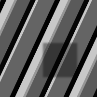
Shadowed ${\bm{f}}$

Orientation angle $\bm{\theta}$

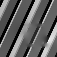
Isotropic osmosis

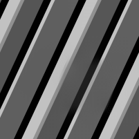
Anisotropic osmosis

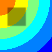
Shadowed ${\bm{f}}$

Orientation angle $\bm{\theta}$

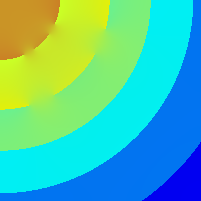
Isotropic osmosis

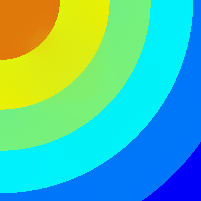
Anisotropic osmosis

Figure 5: Shadow removal via osmosis on synthetic images. Comparison between isotropic and aniotropic osmosis. Parameters: time step size $\tau=100$, final time $T=10000$, and smaller eigenvalue $\varepsilon=0.05$.

4.2 Real-world examples

In order to apply the anisotropic model to natural real-world images, the estimation of the discrete local orientation $\bm{\theta}({\bm{x}})$ becomes crucial. Therefore, we show in Section 4.2.1 the results of the proposed approach discussed in Section 2.3. Once the directions are estimated, we present in Section 4.2.2 the results of the anisotropic osmosis filter on real shadowed images.

4.2.1 Estimation of the local orientation.

Following Section 2.3, here we present the algorithm and the results for estimating the vector field that closes the interrupted lines onto the shadow boundary domain $\Omega_{\text{sb}}$, via the modified tensor voting framework.

For the tensor voting, we used the MATLAB implementation of [12] from the companion software of [23], a literature review on tensor voting. Also, since tensor voting depends on local neighbourhoods, we use a multi-resolution strategy as is described in Algorithm 2.

Input : a shadowed image ${\bm{f}}$ of dimension $M\times N\times C$ (with $C$ colour channels);

a mask with value 1 on shadow boundary and 0 elsewhere;

a stack of $\textnormal{{scales}}=[s_{1},\dots,s_{S}]$;

the parameter $\sigma>0$.

Package : encode and vote from mathworks.com/matlabcentral/fileexchange/47398 modified to return orientation_loc and orientation in $(x,y)$ coordinates

Function estimate_directions:

       TVF = zeros(size(${\bm{f}}$,1),size(${\bm{f}}$,2),2,2);

       for $c=1,\dots,C$ do

             [ saliency_loc, ballness_loc, orientation_loc ] = encode ($K_{\sigma}\ast{\bm{f}}(:,:,c)$);

             // zeroing and randomizing the data on the shadow edges $\Omega_{\text{sb}}$

             saliency_loc = saliency_loc.*mask ;

             orientation_loc = orientation_loc.*mask + $2\pi$.* rand(size(${\bm{f}}(:,:,c)$)).*(1-mask);

             foreach $k$ in scales do

                   [ saliency, ballness, orientation ] = vote ( saliency_loc, orientation_loc,  $s_{k}$ );

                   $\bm{\lambda}_{1}$ = saliency +ballness ;

                   $\bm{\lambda}_{2}$ = ballness ;

                   ${\bm{e}}_{1}$ = ( cos(orientation), sin(orientation));

                   ${\bm{e}}_{2}$ = (-sin(orientation), cos(orientation));

                  

                  TVF = TVF + eigen_to_tensor ( ${\bm{e}}_{1}$, ${\bm{e}}_{2}$, $\bm{\lambda}_{1}$, $\bm{\lambda}_{2}$ );

                  

             end foreach

            

       end for

      [ ${\bm{e}}_{1}$, ${\bm{e}}_{2}$, $\bm{\lambda}_{1}$, $\bm{\lambda}_{2}$ ] = tensor_to_eigen ( TVF );

       $\bm{\theta}$ = xy2ij (${\bm{e}}_{2}$);

        // return the local orientation in $(i,j)$ coordinates

      

return $\bm{\theta}$

Algorithm 2 (Multi-scale) Eigen-directions via tensor voting in shadowed image

In Figure 6 we compare the local direction estimation by means of the structure tensor and the tensor voting approach applied on the shadowed image in Figure 6(a). We plot the magnitude of the leading eigenvalue of the structure tensor in Figure 6(b) and of the one computed for the tensor voting Algorithm 2 in Figure 6(c). These images clearly show that the estimation via tensor voting is less sensitive to the false edges introduced by the shadow boundaries. This is reflected in the plot of the leading directions, too: The directions computed via the structure tensor in Figure 6(d) are visibly affected by the light jumps while the ones computed with tensor voting in Figure 6(e) can still connect the structures from outside to inside the shadow with no additional edges.

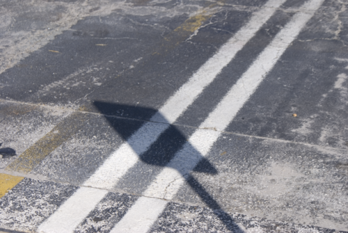
(a) Input ${\bm{f}}$

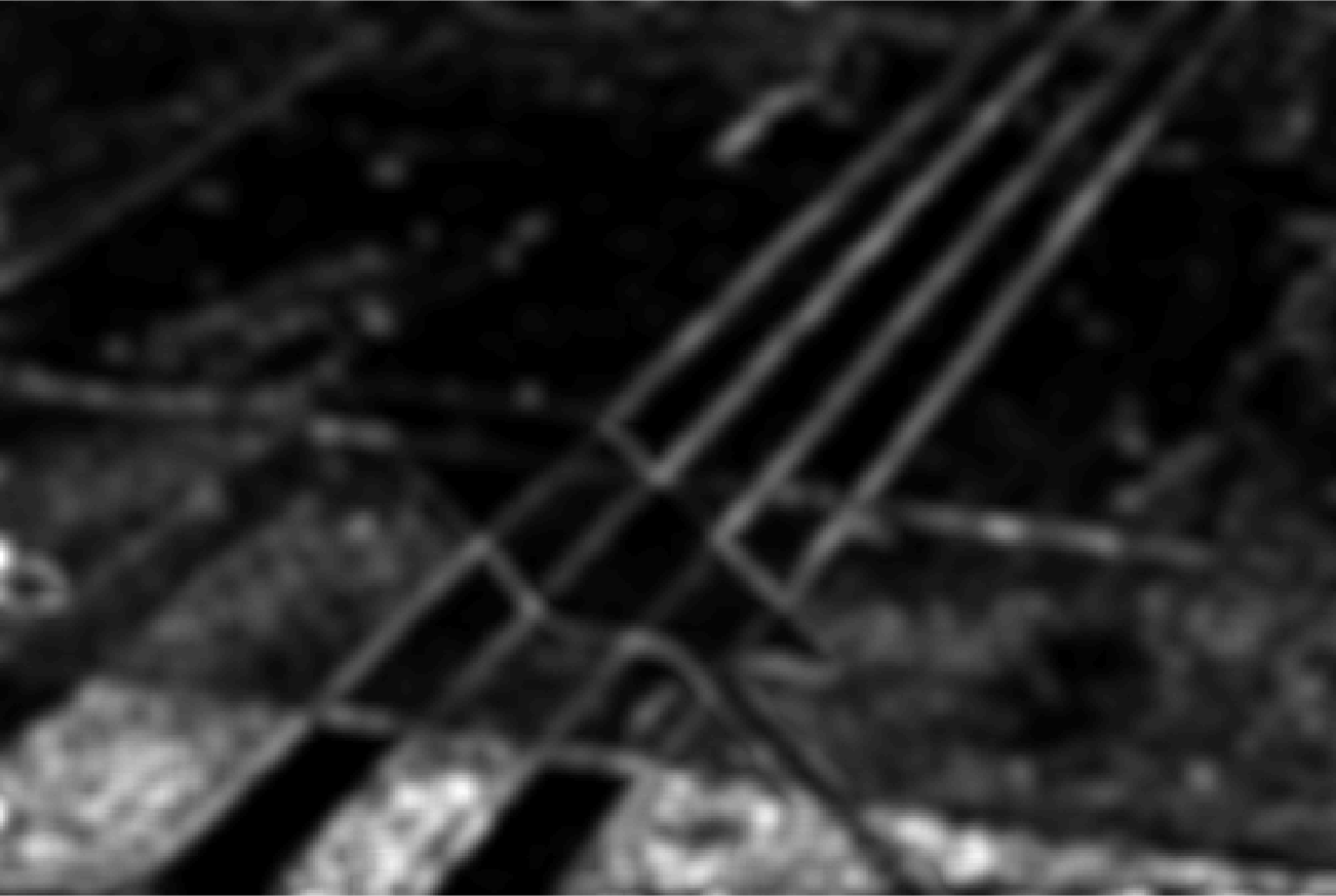
(b) STF, $\bm{\lambda}_{1}$

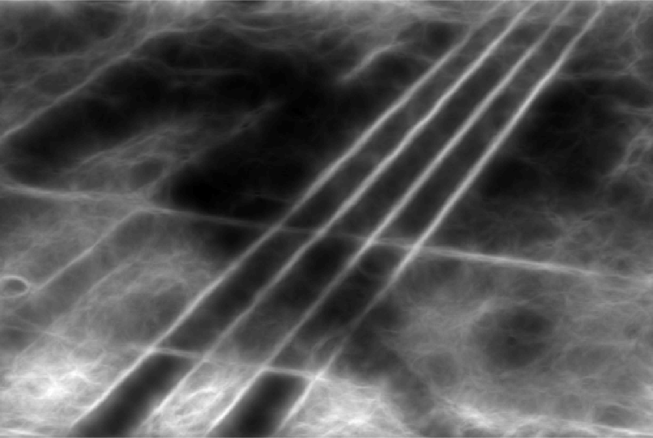
(c) TVF, $\bm{\lambda}_{1}$

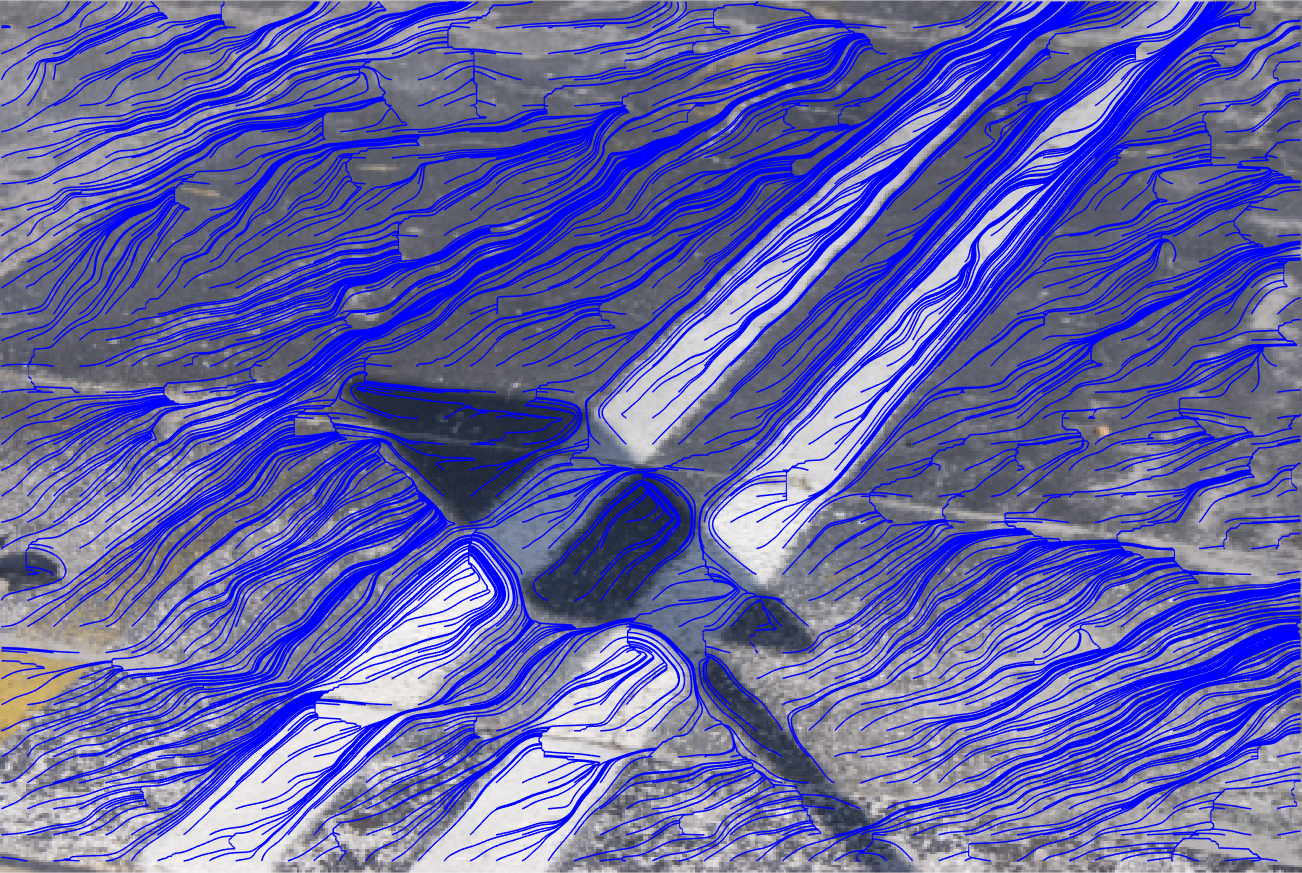
(d) STF, ${\bm{e}}_{1}$

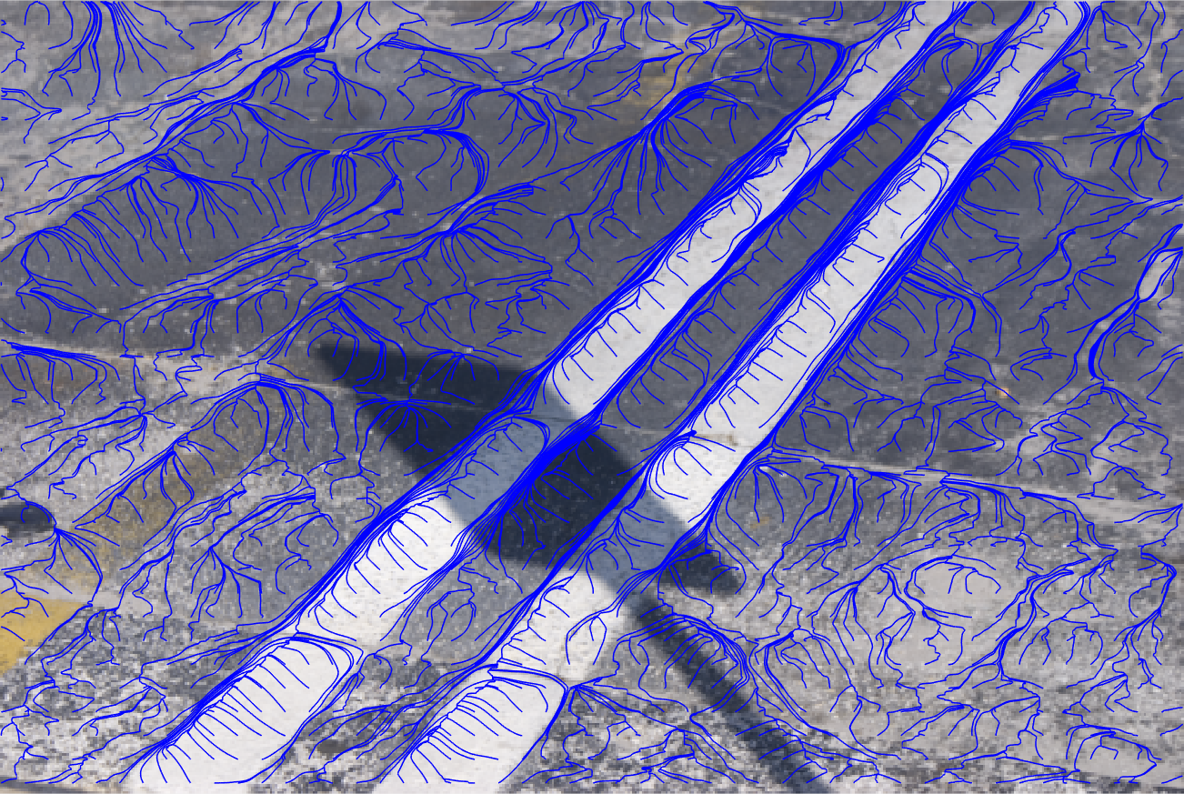
(e) TVF, ${\bm{e}}_{1}$

Figure 6: Comparison: structure tensor framework (STF) with $(\sigma,\rho)=(0.5,4)$ versus tensor voting framework (TVF) with multi-scales $(5,10,15)$ and $\sigma=0.5$. We plot the main direction ${\bm{e}}_{1}$ and its associated eigenvalue $\bm{\lambda}_{1}$.

4.2.2 Results on real images.

We now combine the proposed tensor voting framework with the anisotropic osmosis model to remove constant shadows by means of an anisotropic drift-diffusion model. In the following experiments we use the final time $T=100000$ and the time step size $\tau=1000$. In practice the shadow removal is accomplished almost completely already for $t\ll T$. However, for a better approximation of the steady state, we use the final time $T$ for comparison.

In Figure 7 we show a zoom of the results from Figure 3, presented as motivation for this work. Note that in this case the shadow is artificially added as a multiplicative rescaling factor $c\in(0,1)$. The estimation of the direction on the shadow boundary is computed via the proposed Algorithm 2.

(a) Shadowed ${\bm{f}}$

Orientation angle $\bm{\theta}$

Isotropic

Anisotropic

Figure 7: Zoom of the results for the shadowed image in Figure 3.

In Figure 8 we apply the isotropic and the anisotropic model to a several shadowed images affected by natural constant shadows. Zoomed details can be found in Figure 9. Here the complexity of local image structures makes the application of the anisotropic osmosis model harder. Thus, we use the tensor voting algorithm 2 to estimate the local directions connecting the structures from inside to the outside of the shadow region. Also in these real-world scenarios, we observe the superiority of the anisotropic approach: structures are interpolated reliably across the light jump introduced by the shadow.

(a) Shadowed ${\bm{f}}$

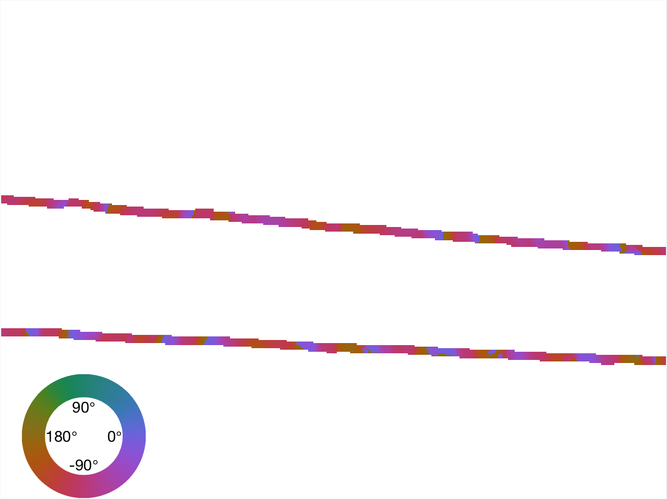
Orientation angle $\bm{\theta}$

Isotropic

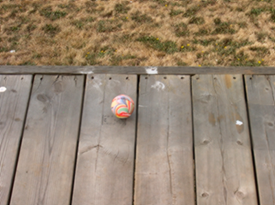
Anisotropic

(b) Shadowed ${\bm{f}}$

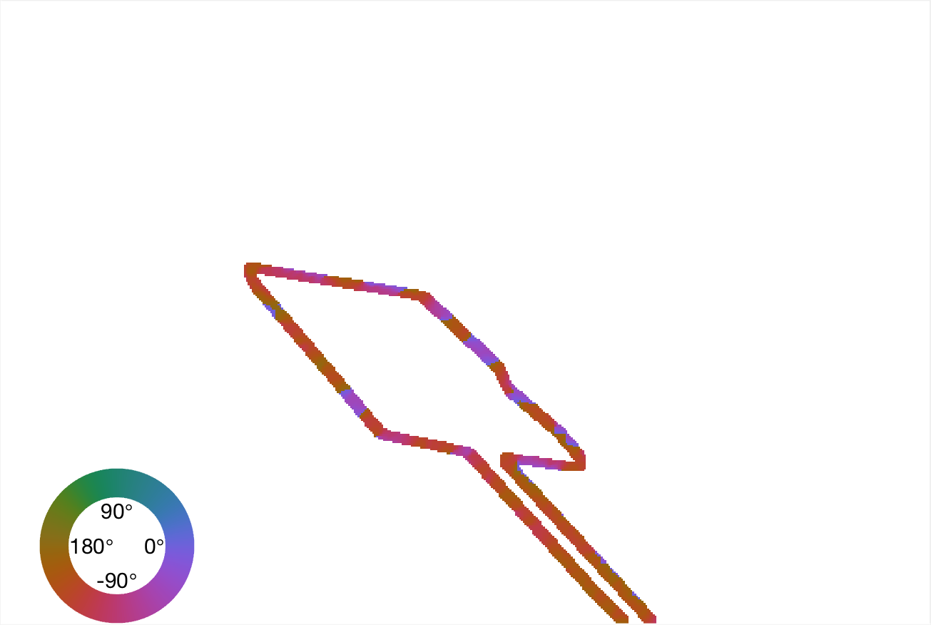
Orientation angle $\bm{\theta}$

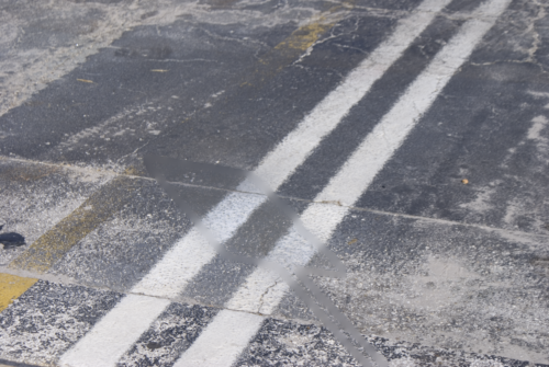
Isotropic

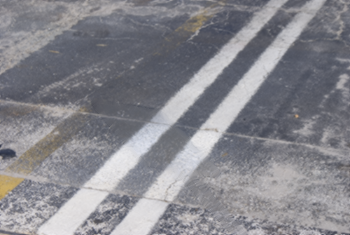
Anisotropic

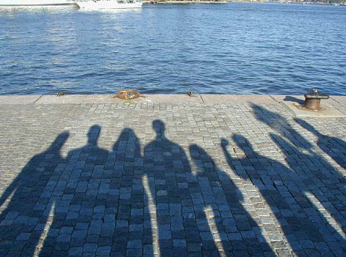
(c) Shadowed ${\bm{f}}$

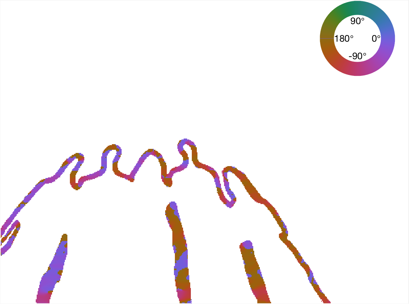
Orientation angle $\bm{\theta}$

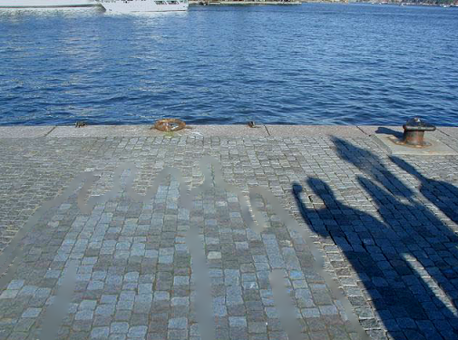
Isotropic

Anisotropic

Figure 8: Shadow removal via osmosis on real images. Comparison between isotropic and anisotropic osmosis. Parameters: $\tau=1000$, $T=100000$, $\varepsilon=0.05$, and $\sigma=0.5$.

(a) Isotropic

(b) Anisotropic

(c) Isotropic

(d) Anisotropic

(e) Isotropic

(f) Anisotropic

Figure 9: Zoom into the results from Figure 8.

4.3 Comments on the results

We note that our anisotropic approach removes shadows effectively both for synthetic and real-world images. Structures are propagated correctly over the shadow boundary.

Since the AD-LBR stencil requires a positive definite matrix $\mathbf{W}$ as input, we need to choose $\varepsilon>0$, which may lead to some over-smoothing in the orthogonal direction. Also, we noticed some over-smoothing effect in $\Omega_{\text{out}}$ and $\Omega_{\text{in}}$ for the AD-LBR scheme, e.g.  in Figure 9(f), whose understanding is a matter of future research.

In terms of efficiency, the computational time needed for computing the action of the exponential matrix onto a vector, that is the product $\exp(\tau\mathbf{A}){\bm{u}}^{0}$, largely depends on the choice of the time-step $\tau$, the final time $T$ and the size of the images. Although it is possible to directly choose $\tau=T$ and proceed in a single step, we prefer multiple steps. In this way, by comparing two successive solutions ${\bm{u}}^{k+1}$ and ${\bm{u}}^{k}$, it is possible to detect whether the evolution is sufficiently close to its steady state. Our solvers that are exact in time offer additional advantages over classical inexact methods such as explicit and implicit schemes when one is also interested in good approximations of intermediate results.

5 Conclusions and outlook

In this work, we have generalised isotropic osmosis filtering introduced in [36, 38] to the anisotropic setting. This was achieved by introducing a weight matrix whose directional information was extracted from a modified tensor voting approach [24]. When applied to the shadow removal problem, the anisotropic model acts as an inpainting interpolator on the shadow boundary. It is close in spirit to inpainting with edge-enhancing anisotropic diffusion [39, 13, 33].

From a numerical point of view, we have combined the nonnegativity preserving anisotropic diffusion stencil of Fehrenbach and Mirebeau [10] with techniques based on exponential integration [6]: We argued that the fully discrete model satisfies the discrete properties studied in [36] in a general setting for osmosis. We tested the proposed model for synthetic and real examples, showing that the generalised model acts as a combined osmosis-inpainting model for shadow removal problems, thus avoiding any undesirable post-processing inpainting step.

Future work will address the investigation on the applicability of the proposed anisotropic model to more general imaging applications.

References

References

- [1] Al-Mohy, A.H., Higham, N.J.: Computing the action of the matrix exponential with an application to exponential integrators. SIAM Journal on Scientific Computing 33(2), 488–511 (2011). DOI 10.1137/100788860
- [2] Arias, P., Facciolo, G., Caselles, V., Sapiro, G.: A variational framework for exemplar-based image inpainting. International Journal of Computer Vision 93(3), 319–347 (2011). DOI 10.1007/s11263-010-0418-7
- [3] Aubert, G., Kornprobst, P.: Mathematical problems in image processing: Partial Differential Equations and the Calculus of Variations, vol. 147. Springer-Verlag, New York (2006). DOI 10.1007/978-0-387-44588-5
- [4] Baba, M., Asada, N.: Shadow removal from a real picture. In: ACM SIGGRAPH 2003 Sketches & Applications, SIGGRAPH ’03, pp. 1–1. ACM, New York, NY, USA (2003). DOI 10.1145/965400.965488
- [5] Calatroni, L., Estatico, C., Garibaldi, N., Parisotto, S.: Alternating direction implicit (ADI) schemes for a PDE-based image osmosis model. Journal of Physics: Conference Series 904(1), 012,014 (2017). DOI 10.1088/1742-6596/904/1/012014
- [6] Caliari, M., Kandolf, P., Ostermann, A., Rainer, S.: The Leja method revisited: Backward error analysis for the matrix exponential. SIAM Journal on Scientific Computing 38(3), A1639–A1661 (2016). DOI 10.1137/15M1027620
- [7] Chan, T., Shen, J.: Image Processing and Analysis: Variational, PDE, Wavelet, and Stochastic Methods. Society for Industrial and Applied Mathematics, Philadelphia (2005). DOI 10.1137/1.9780898717877
- [8] Chunxia, X., Ruiyun, S., Donglin, X., Kwanâ-Liu, M.: Fast shadow removal using adaptive multi-scale illumination transfer. Computer Graphics Forum 32(8), 207–218 (2013). DOI 10.1111/cgf.12198
- [9] Conway, J.H., Sloane, N.J.A.: Low-dimensional lattices. vi. Voronoi reduction of three-dimensional lattices. Proceedings of the Royal Society of London A: Mathematical, Physical and Engineering Sciences 436(1896), 55–68 (1992). DOI 10.1098/rspa.1992.0004
- [10] Fehrenbach, J., Mirebeau, J.M.: Sparse non-negative stencils for anisotropic diffusion. Journal of Mathematical Imaging and Vision 49(1), 123–147 (2014). DOI 10.1007/s10851-013-0446-3
- [11] Förstner, W.: A Feature Based Correspondence Algorithm for Image Matching. Int. Arch. of Photogrammetry and Remote Sensing 26(3), 150–166 (1986)
- [12] Franken, E., van Almsick, M., Rongen, P., Florack, L., ter Haar Romeny, B.: An efficient method for tensor voting using steerable filters. In: A. Leonardis, H. Bischof, A. Pinz (eds.) Computer Vision - ECCV 2006, pp. 228–240. Springer Berlin Heidelberg, Berlin, Heidelberg (2006). DOI 10.1007/11744085˙18
- [13] Galić, I., Weickert, J., Welk, M., Bruhn, A., Belyaev, A., Seidel, H.P.: Image compression with anisotropic diffusion. Journal of Mathematical Imaging and Vision 31(2–3), 255–269 (2008). DOI 10.1007/s10851-008-0087-0
- [14] Grasmair, M., Lenzen, F.: Anisotropic total variation filtering. Applied Mathematics and Optmization 62, 323–339 (2010). DOI 10.1007/s00245-010-9105-x
- [15] Guichard, F., Moisan, L., Morel, J.M.: A review of PDE models in image processing and image analysis. Journal de Physique IV pp. 137–154 (2002). DOI 10.1051/jp42002006
- [16] Guy, G., Medioni, G.: Inferring global perceptual contours from local features. International Journal of Computer Vision 20(1), 113–133 (1996). DOI 10.1007/BF00144119
- [17] Hagenburg, K., Breuß, M., Weickert, J., Vogel, O.: Novel schemes for hyperbolic pdes using osmosis filters from visual computing. In: A.M. Bruckstein, B.M. ter Haar Romeny, A.M. Bronstein, M.M. Bronstein (eds.) Scale Space and Variational Methods in Computer Vision, pp. 532–543. Springer, Berlin (2012). DOI 10.1007/978-3-642-24785-9˙45
- [18] Harris, C., Stephens, M.: A combined corner and edge detector. In: Proceedings of the Alvey Vision Conference, pp. 23.1–23.6. Alvety Vision Club (1988). DOI 10.5244/C.2.23
- [19] Hochbruck, M., Ostermann, A.: Exponential integrators. Acta Numerica 19, 209–286 (2010). DOI 10.1017/S0962492910000048
- [20] Kass, M., Witkin, A.: Analyzing oriented patterns. Computer Vision, Graphics, and Image Processing 37(3), 362 – 385 (1987). DOI 10.1016/0734-189X(87)90043-0
- [21] Kongskov, R.D., Dong, Y.: Directional total generalized variation regularization for impulse noise removal. In: F. Lauze, Y. Dong, A.B. Dahl (eds.) Scale Space and Variational Methods in Computer Vision, pp. 221–231. Springer International Publishing, Cham (2017). DOI 10.1007/978-3-319-58771-4˙18
- [22] Kongskov, R.D., Dong, Y., Knudsen, K.: Directional total generalized variation regularization (2017). ArXiv preprint: 1701.02675
- [23] Maggiori, E., Manterola, H.L., del Fresno, M.: Perceptual grouping by tensor voting: a comparative survey of recent approaches. IET Computer Vision 9(2), 259–277 (2015). DOI 10.1049/iet-cvi.2014.0103
- [24] Moreno, R., Pizarro, L., Burgeth, B., Weickert, J., Garcia, M.A., Puig, D.: Adaptation of tensor voting to image structure estimation. In: D.H. Laidlaw, A. Vilanova (eds.) New Developments in the Visualization and Processing of Tensor Fields, pp. 29–50. Springer (2012)
- [25] Mrázek, P., Navara, M.: Consistent positive directional splitting of anisotropic diffusion. In: B. Likar (ed.) Proc. Sixth Computer Vision Winter Workshop, pp. 37–48. Bled, Slovenia (2001)
- [26] Nagel, H.H., Enkelmann, W.: An investigation of smoothness constraints for the estimation of displacement vector fields from image sequences. IEEE Trans. Pattern Anal. Mach. Intell. 8(5), 565–593 (1986). DOI 10.1109/TPAMI.1986.4767833
- [27] Parisotto, S., Calatroni, L., Daffara, C.: Digital cultural heritage imaging via osmosis filtering. In: A. Mansouri, A. El Moataz, F. Nouboud, D. Mammass (eds.) Image and Signal Processing LNCS 10884, pp. 407–415. Springer International Publishing, Cham (2018). DOI 10.1007/978-3-319-94211-7˙44
- [28] Parisotto, S., Masnou, S., Schönlieb, C.B.: Higher order total directional variation. Part I: Imaging applications (forthcoming)
- [29] Parisotto, S., Masnou, S., Schönlieb, C.B.: Higher order total directional variation. Part II: Analysis (forthcoming)
- [30] Protter, M.H., Weinberger, H.F.: Maximum Principles in Differential Equations. Springer-Verlag New York (1984). DOI 10.1007/978-1-4612-5282-5
- [31] Saad, Y.: Analysis of some Krylov subspace approximations to the matrix exponential operator. SIAM Journal on Numerical Analysis 29 (1992). DOI 10.1137/0729014
- [32] Sapiro, G.: Geometric Partial Differential Equations and Image Analysis. Cambridge University Press, Cambridge, UK (2001). DOI 10.1017/CBO9780511626319
- [33] Schmaltz, C., Peter, P., Mainberger, M., Ebel, F., Weickert, J., Bruhn, A.: Understanding, optimising, and extending data compression with anisotropic diffusion. International Journal of Computer Vision 108(3), 222–240 (2014). DOI 10.1007/s11263-014-0702-z
- [34] Schönlieb, C.B.: Partial Differential Equation Methods for Image Inpainting. Cambridge Monographs on Applied and Computational Mathematics. Cambridge University Press (2015). DOI 10.1017/CBO9780511734304
- [35] Tarjan, R.: Depth-first search and linear graph algorithms (1972). DOI 10.1137/0201010
- [36] Vogel, O., Hagenburg, K., Weickert, J., Setzer, S.: A fully discrete theory for linear osmosis filtering. In: A. Kuijper, K. Bredies, T. Pock, H. Bischof (eds.) Scale Space and Variational Methods in Computer Vision, pp. 368–379. Springer Berlin Heidelberg, Berlin, Heidelberg (2013). DOI 10.1007/978-3-642-38267-3˙31
- [37] Weickert, J.: Anisotropic Diffusion in Image Processing. B.G. Teubner, Stuttgart (1998)
- [38] Weickert, J., Hagenburg, K., Breuß, M., Vogel, O.: Linear osmosis models for visual computing. In: A. Heyden, F. Kahl, C. Olsson, M. Oskarsson, X.C. Tai (eds.) Energy Minimization Methods in Computer Vision and Pattern Recognition, pp. 26–39. Springer Berlin Heidelberg, Berlin, Heidelberg (2013). DOI 10.1007/978-3-642-40395-8˙3
- [39] Weickert, J., Welk, M.: Tensor field interpolation with PDEs. In: J. Weickert, H. Hagen (eds.) Visualization and Processing of Tensor Fields, pp. 315–325. Springer, Berlin (2006). DOI 10.1007/3-540-31272-2˙19
- [40] Weickert, J., Welk, M., Wickert, M.: L2-stable nonstandard finite differences for anisotropic diffusion. In: A. Kuijper, K. Bredies, T. Pock, H. Bischof (eds.) Scale Space and Variational Methods in Computer Vision, pp. 380–391. Springer Berlin Heidelberg, Berlin, Heidelberg (2013). DOI 10.1007/978-3-540-72823-8