Globally Optimal AC Power System Upgrade Planning under Operational Policy Constraints

Abstract

In order to accommodate the increasing amounts of renewable generation in power distribution systems, system operators are facing the problem of how to upgrade transmission capacities.

Since line and transformer upgrades are costly, optimization procedures are used to find the minimal number of upgrades required.

The resulting design optimization formulations are generally mixed-integer non-convex problems.

Traditional approaches to solving them are usually of a heuristic nature, yielding no bounds on suboptimality or even termination.

In contrast, this work combines heuristics, lower-bounding procedures and practical operational policy constraints.

The resulting algorithm finds both suboptimal solutions quickly and the global solution deterministically by a Branch-and-Bound procedure augmented with lazy cuts.

1 Introduction

Increased penetration of renewables in distribution systems is leading to voltage violations at peak generation times [1]. Both changes to the operational schemes of the systems [2] as well as changes to the system topologies themselves [3] are being investigated as remedies to these problems. This work treats the particular problem of selecting which lines of a power grid to upgrade in order to stop voltage violations from recurring in the future. Since significant investments are required for infrastructure upgrades, optimization for minimum cost is desired.

Power system planning optimizations based on the AC model of the system generally lead to non-convex optimization problems due to the non-linearity of the equations involved. Additionally, integrality is introduced into the planning problems from two sources: Firstly, the number of lines to be upgraded is usually the dominant factor in the cost. This leads to a cardinality-type cost that can be formulated using binary variables. Secondly, there are often only a given number of different line admittance values available for purchase. The presence of this integrality can be modeled with integer decision variables. Due to the integrality and non-convexity of the problem, most existing methods for solving it are heuristic in nature. One line of research applies stochastic algorithms to the problem [4]. Another approach is to approximate the system model by the DC power flow equations [5], turning the mixed-integer nonlinear program (MINLP) into a mixed-integer linear program (MILP). Mature codes for solving the latter are commercially available. However, the solution of the MILP approximation is not necessarily feasible for the original MINLP. A third approach is to form a convex outer approximation of the non-convex AC model based on conic constraints, leading to a mixed-integer semidefinite problem (MISDP) [6]. Compared to the DC power flow approximation, this approach has the advantage of yielding a guaranteed lower bound on the optimal cost of the planning problem.

The method presented in this paper extends the third approach based on MISDP in two aspects: Firstly, additional constraints are added to the problem that specify how the system will be operated given fixed upgrade decisions and load patterns. These constraints will hereafter be referred to as “policy constraints”. The addition of policy constraints guarantees that the solution of the planning problem is feasible when deployed in practice. Additionally it circumvents the difficulty of checking feasibility of a power flow for a given load pattern, which was recently shown to be NP-hard [7, 8]. Secondly, the Branch-and-Bound algorithm is adapted to incorporate the policy constraints efficiently. The result is a method that deterministically finds the globally optimal solution for an optimization problem that better reflects reality than the commonly used MINLP without policy constraints. Due to the nature of the Branch-and-Bound procedure, any existing heuristics for finding useful feasible points as well as existing lower-bounding methods can easily be integrated into the approach. Despite the problem still being NP-hard to solve, the numerical experiments presented towards the end of the paper demonstrate that the method can be applied successfully to practical systems.

1.1 Outline

Section 2 introduces notation, the model, policy constraints and violating snapshots. It ends with a formulation of the upgrade problem solved in this work. Section 3 introduces the Branch-and-Bound algorithm used and the implementation of policy constraints as lazy cuts. Section 4 presents numerical simulations with different operating policies and discusses properties of the results.

2 Modeling

2.1 Notation and Kirchhoff equations

The complex conjugate of a complex variable $x$ is denoted by $\bar{x}$. We will use tuple notation $(a,b)$ where appropriate to refer to a collection of vectors $a$ and $b$ to avoid introducing overly many stacked vectors. The power grid is modeled using an undirected graph with $N$ vertices (representing buses) and $L$ edges (representing lines). Each line (say, between buses $j$ and $l$) has an admittance $y_{jl}\in\mathbb{C}$. Associated with each bus $j$ is a voltage $v_{j}\in\mathbb{C}$ and a power in-feed $s_{j}\in\mathbb{C}$. The power flows in the grid are governed by the AC Kirchhoff equations:

$$\operatorname{diag}(v)\bar{Y}\bar{v}=s,$$ (1)

where $Y\in\mathbb{C}^{N\times N}$ is the system admittance matrix:

$$Y_{jl}:=\begin{cases}y_{jl}&\text{if }j\neq l,\\ y_{j}^{\mathrm{sh}}-\sum_{k=1,k\neq j}^{N}y_{jk}&\text{if }j=l,\end{cases}$$ (2)

with $y_{j}^{\mathrm{sh}}\in\mathbb{C}$ being shunt admittances.

2.2 Operation-independent constraints

Certain constraints are needed no matter how the system is operated. Firstly, the voltage magnitude at each bus $j$ is constrained to an admissible range:

$$v_{\min,j}\leq|v_{j}|\leq v_{\max,j},$$ (3)

and the currents over the lines (for example, line $(l,j)$) are constrained to be within thermal limits:

$$|Y_{jl}||v_{j}-v_{l}|\leq I_{\max,jl}.$$ (4)

Assume the power at each bus $j$ has upper and lower bounds:

$$s_{\min,j}\leq s_{j}\leq s_{\max,j},$$ (5)

which can be interpreted as generator capability bounds for generator buses. At load buses, the bounds can either represent the capability for demand response or they can be fixed to the specific load drawn at that bus in a given scenario. For ease of notation, define the set of voltages and powers satisfying these constraints as

$$\mathcal{X}:=\left\{(s,v)\;\big{|}\;\eqref{eqn:vdonut},\eqref{eqn:linecurr},\eqref{eqn:powbox}\right\}.$$ (6)

In the case of multiple distinct system states being considered, we will make use of the notation $\mathcal{X}^{k}$ for the constraints applying for system state $k$. Note that the set $\mathcal{X}$ is parametrized by $Y$ and $I_{\max,jl}$.

Additional constraints can be included in the approach provided they admit semidefinite relaxations and can be included in the policy. For example, one way of including phase angle constraints is in the form of

$$\left|v_{j}-v_{l}\right|^{2}\leq\sin(\alpha)^{2}\left|v_{j}\right|,$$ (7)

for a line from bus $j$ to bus $l$ and an angle limit of $\alpha$. Constraint (7) can be added to the problem in quadratic form and handled similarly to the voltage magnitude constraints.

2.3 Operational policy

Assume now that the buses of the network are partitioned into loads and generators. Accordingly, let $s_{\mathrm{gen}}$ be the vector of powers of the generators and $s_{\mathrm{load}}$ be that of the loads. Given a system topology and load pattern, we assume the operator of the generators picks set-points (and with them, the network voltages) based on a given operating policy:

$$(s_{\mathrm{gen}},v)=g(Y,s_{\mathrm{load}}).$$ (8)

Note that we make the distinction between variables that are under operator control (specifically $s_{\mathrm{gen}}$ and by extension also $v$ here) and variables the operator can only measure or estimate (specifically $s_{\mathrm{load}}$ here). The method presented in this work does not require this specific distinction, only that a distinction is made. One could for example also include curtailable loads in the set of variables under operator control.

The operating policy function $g$ can be any surjective function, the only requirement is that it can be evaluated with reasonable efficiency. Examples for operational policies include:

• Local frequency-based controllers at the generators;

• Networked frequency-based controllers;

• Power flow computations with fixed generator voltages;

• Numerical economic dispatch computations.

Note that in all these operational policies, the resulting system state $(s,v)$ has to satisfy the Kirchhoff equations (1) in order to be physically meaningful. However, whether $(s,v)$ is in $\mathcal{X}$ or not can depend on the policy. For example, it could happen that while local controllers might not find a workable solution for a situation in which the system is strongly loaded, numerical optimization methods can.

2.4 Line upgrades

Line upgrades are modeled as changes to the Laplacian matrix $Y$ of the grid: For each upgrade, a binary variable $a_{i}$ encodes whether the upgrade is performed ($1$) or not ($0$). A constant matrix $\delta Y_{i}\in\mathbb{C}^{N\times N}$ is used to encode the change this upgrade brings to the system. Overall, the upgraded $Y$ can then be written as follows:

$$Y_{\mathrm{upg}}=Y+\sum_{i=1}^{n_{u}}(a_{i}\cdot\delta Y_{i}),$$ (9)

where $n_{u}$ is the number of upgrade possibilities. This formulation allows for multiple line upgrades to be linked into one upgrade possibility as well as for shunt admittance changes. The upgrade variables are now collected in a vector $a\in\{0,1\}^{n_{u}}$ and are assumed to be the only influence on system topology in the problem.

The change in the line current limits introduced by the upgrades is similarly defined as

$$I_{\max,jl,\mathrm{upg}}=I_{\max,jl}+\sum_{i\in\mathcal{U}_{jl}}(a_{i}\cdot\delta I_{jl,i}),$$ (10)

where $\mathcal{U}_{jl}$ is the set of upgrade indices that affect the line from bus $j$ to bus $l$ and $\delta I_{jl,i}$ is the change in current limit introduced to that line by the upgrade $i$.

2.5 Violating snapshots

We assume that a set of problematic steady-state snapshots $(s^{k},v^{k})$, $k\in\{1,\ldots,K\}$ are given. These snapshots are assumed to satisfy the Kirchhoff equations (1), but violate some of the voltage and current constraints in (3) and (4). Snapshot data can come from a variety of sources: Examples include past measurement data, predictions of future scenarios or known worst case loadings. It is useful to look at past violating snapshots due to the repetitiveness of load patterns: If a violating load pattern is observed, it is likely that a similar pattern will show up again in the future. The assumption is made here that the uncertainty and variability of renewables is represented adequately by the selection and number of snapshots. A more precise representation of uncertainty is difficult to formulate at this time due to the non-convexity of the upgrade problem and the presence of policy constraints.

2.6 System upgrade problem

The problem we address in this work is to find upgrades to the power system that would eliminate all constraint violations in the considered snapshots by means of grid upgrades. The problem we would like to solve can be written as follows:

Problem U: $$\;\;\operatorname*{minimize}_{a,\tilde{v}^{k},\tilde{s}^{k}}\;\;f(a)$$ (U.1)

$$\operatorname*{subject\ to} \;\;Aa\leq b$$ (U.2)

$$\;\;a\in\{0,1\}^{n_{u}}$$ (U.3)

$$\;\;Y_{\mathrm{upg}}=Y+\sum_{i=1}^{n_{u}}(a_{i}\cdot\delta Y_{i})$$ (U.4)

$$\;\;I_{\max,jl,\mathrm{upg}}=I_{\max,jl}+\sum_{i\in\mathcal{U}_{jl}}(a_{i}\cdot\delta I_{jl,i}),$$ (U.5)

$$\;\;\operatorname{diag}(\tilde{v}^{k})\overline{Y_{\mathrm{upg}}\tilde{v}^{k}}=\tilde{s}^{k}$$ (U.6)

$$\;\;(\tilde{s}^{k},\tilde{v}^{k})\in\mathcal{X}^{k}$$ (U.7)

$$\;\;(s_{\mathrm{gen}}^{k},v^{k})=g(Y_{\mathrm{upg}},s_{\mathrm{load}}^{k})$$ (U.8)

$$\;\;\forall k\in\{1,\ldots,K\},$$

where $f(a)$ represents the cost of the upgrades and is assumed here to be convex. Convexity of $f(a)$ is required for the branch and bound procedure to work. The polyhedron $Aa\leq b$ represents constraints on upgrade combinations – for example that only one line type can be chosen per location. Note also that given a value for $a$, the value of $Y_{\mathrm{upg}}$ can be computed using (U.4). Therefore, the policy can also be understood as being a function of $a$ directly and we will use the more compact notation $g(a,s_{\mathrm{load}})$ from now on. The variable vectors $\tilde{s}^{k}$ and $\tilde{v}^{k}$ are defined as follows:

$$\tilde{s}^{k}_{i}=\begin{cases}s^{k}_{i}&\text{if bus $i$ is a load}\\ \text{a decision variable}&\text{otherwise.}\\ \end{cases}$$ (12)

The voltage vector $\tilde{v}^{k}$ is entirely an optimization variable: We expect all voltages in the network to change if the topology and dispatch change. For PV buses, the magnitude can be fixed by setting the lower and upper limits appropriately. While it may seem like the presence of the constraint (U.7) renders the Kirchhoff constraint (U.6) irrelevant, the latter will become important later on for relaxation purposes.

3 Branch-and-Bound procedure including policy constraints

3.1 QCQP formulation and semidefinite relaxation

For the sake of easier notation, we assume there is only one snapshot (i.e., $K=1$) and omit the $k$ index in this section. The resulting reformulation then applies to each snapshot $k$ separately. As shown in [6, 9], among others, it is possible to apply a set of reformulations to the intersection of the constraints (U.4) through (U.7). The result of these reformulations is a set of quadratic constraints

$$\alpha_{i}\leq z^{T}Q_{i}z+q_{i}^{T}y+m_{i}^{T}a\leq\beta_{i}$$ (13)

for $i\in\{1,\ldots,I\}$ and where $z$ contains the voltage variables ($z=\begin{bmatrix}\operatorname{Re}{v}^{T}&\operatorname{Im}{v}^{T}\end{bmatrix}^{T}$), $a$ contains the upgrade variables as before and $y$ contains all the remaining variables. The latter include the generator powers as well as additional variables that were introduced in the reformulation. A detailed outline of the reformulation used in this work is omitted here for brevity but can be found in [10]. This means problem (11) can be equivalently rewritten as

Problem P: $$\;\;\operatorname*{minimize}_{a,z,y}f(a)$$ (P.1)

$$\operatorname*{subject\ to} \;\;Aa\leq b$$ (P.2)

$$\;\;a\in\{0,1\}^{n_{u}}$$ (P.3)

$$\;\;\alpha_{i}\leq z^{T}Q_{i}z+q_{i}^{T}y+m_{i}^{T}a\leq\beta_{i}$$ (P.4)

$$\;\;(s_{\mathrm{gen}},v)=g(a,s_{\mathrm{load}})$$ (P.5)

$$\;\;\forall i\in\{1,\ldots,I\}.$$

A mixed-integer convex relaxation of (14) can be found by applying the commonly used semidefinite relaxation procedure for quadratic constraints, which is outlined in [11], as well as omitting the policy constraint. This leads to a mixed-integer semidefinite problem:

Problem R: $$\;\;\operatorname*{minimize}_{a,Z,y}f(a)$$ (R.1)

$$\operatorname*{subject\ to} \;\;Aa\leq b$$ (R.2)

$$\;\;a\in\{0,1\}^{n_{u}}$$ (R.3)

$$\;\;\alpha_{i}\leq tr(Q_{i}^{T}Z)+q_{i}^{T}y+m_{i}^{T}a\leq\beta_{i}$$ (R.4)

$$\;\;Z\succeq 0$$ (R.5)

$$\;\;\forall i\in\{1,\ldots,I\},$$

where $Z$ represents $zz^{T}$, but relaxed to $Z\succeq 0$ (details on this relaxation are in [11], among others). Problem (15) can now be solved to global optimality using the Branch-and-Bound method, as demonstrated in [6].

3.2 Policy cuts

While computable, the solution of (15) (denoted by $(a^{r},Z^{r},y^{r})$) is not guaranteed to be feasible for (14) due to the former being a relaxation of the latter. Additionally, even if a $z^{r}$ can be found such that $Z^{r}=(z^{r})(z^{r})^{T}$ and $(a^{r},z^{r},y^{r})$ satisfies constraints (P.2) through (P.4), there is no guarantee that the (likely different) operating point that results when the operating policy $g(a^{r},s^{r}_{\mathrm{load}})$ is applied still satisfies them. Assume that we are given a solution $(a^{r},z^{r},y^{r})$ of (15) which is not feasible for (14). A constraint (or “cut”) can then be added to (15) that excludes this particular upgrade choice $a^{r}$:

$$\|a-a^{r}\|_{1}\geq 1,$$ (16)

The cut (16) only removes the particular case $a=a^{r}$ from the feasible space of (15) due to the entries of $a$ being in $\{0,1\}$. Such constraints will hereafter be referred to as “policy cuts”. They can be implemented as linear constraints on $a$. For notational convenience, define the projection of the feasible set of (14) onto the upgrade space as follows:

$$\mathcal{F}_{\eqref{eqn:upgradeproblem2}}:=\left\{a\in\{0,1\}^{n_{u}}\;\middle|\;\begin{matrix}Aa\leq b,\\ \exists(z,y,v,s_{\mathrm{gen}}):\eqref{eqn:up2_quad},\eqref{eqn:oppol}\\ \forall i\in\{1,\ldots,I\}\end{matrix}\right\}.$$ (17)

In other words, $\mathcal{F}_{\eqref{eqn:upgradeproblem2}}$ is the set of all upgrade configurations $a$ for which (14) is feasible. Similarly, for (15), we define

$$\mathcal{F}_{\eqref{eqn:upgradeproblem_cvx}}:=\left\{a\in\{0,1\}^{n_{u}}\;\middle|\;\begin{matrix}Aa\leq b,\\ \exists(Z,y):\eqref{eqn:up3_lmi},\eqref{eqn:up3_psd}\\ \forall i\in\{1,\ldots,I\}\end{matrix}\right\}.$$ (18)

We now state a theorem that relates policy cuts and problems (14) and (15):

Theorem 1.

Let (R⁺) be problem (15) with additional constraints (16) added for each $a^{r}\in\mathcal{A}$, where

$$\mathcal{A}:=\left\{a\in\{0,1\}^{n_{u}}\;\middle|\;a\in\mathcal{F}_{\eqref{eqn:upgradeproblem_cvx}}\setminus\mathcal{F}_{\eqref{eqn:upgradeproblem2}}\right\}.$$

Let $\mathcal{P}$ be the intersection of these constraints, which is a finite-dimensional convex polyhedron:

$$\mathcal{P}:=\left\{a\in\mathbb{R}^{n_{u}}\;\middle|\;\|a-a^{r}\|_{1}\geq 1\;\forall a^{r}\in\mathcal{A}\right\}.$$

This allows the projection of the feasible region of (R⁺) onto the upgrade space to be written as

$$\mathcal{F}_{\text{\emph{(R${}^{+}$)}}}:=\mathcal{F}_{\eqref{eqn:upgradeproblem_cvx}}\cap\mathcal{P}.$$

Problem (R⁺) is now equivalent to (14) in the following sense: $a\in\mathcal{F}_{\eqref{eqn:upgradeproblem2}}$ if and only if $a\in\mathcal{F}_{\text{\emph{(R${}^{+}$)}}}$. Additionally, (R⁺) and (14) have the same sets of globally optimal choices of $a$.

Proof.

First note that $\mathcal{F}_{\eqref{eqn:upgradeproblem2}}\subseteq\mathcal{F}_{\eqref{eqn:upgradeproblem_cvx}}$: An optimizer $(a^{*},z^{*},y^{*})$ of (14) can be used to compute a $Z^{*}=(z^{*})(z^{*})^{T}$. This $Z^{*}$ is positive semidefinite and hence $(a^{*},Z^{*},y^{*})$ is feasible for (15). However, any $a$ that are in $\mathcal{F}_{\eqref{eqn:upgradeproblem_cvx}}\setminus\mathcal{F}_{\eqref{eqn:upgradeproblem2}}$ are excluded from (R⁺) by the additional constraints in $\mathcal{P}$, in other words:

$$\mathcal{F}_{\text{(R${}^{+}$)}}=\mathcal{F}_{\eqref{eqn:upgradeproblem_cvx}}\setminus(\mathcal{F}_{\eqref{eqn:upgradeproblem_cvx}}\setminus\mathcal{F}_{\eqref{eqn:upgradeproblem2}})=\mathcal{F}_{\eqref{eqn:upgradeproblem2}}.$$

Because the two problems have the same feasible sets of $a$ and the cost functions are the same and only depend on $a$, the two problems are equivalent. ∎

3.3 Algorithm

1:Set $U=\infty,L=-\infty$, Tree: Root vertex $\mathcal{I}_{0}=\mathcal{I}_{1}=\emptyset$

2:while $U-L>\varepsilon$ do

3:    Pick an unprocessed vertex $\mathcal{N}$ with index sets $\mathcal{I}_{0}^{\mathcal{N}}$, $\mathcal{I}_{1}^{\mathcal{N}}$

4:    Solve (15) with (R.3) replaced by

$$a_{i}\in\begin{cases}\{0\},&\text{if }i\in\mathcal{I}_{0}^{\mathcal{N}},\\ \{1\},&\text{if }i\in\mathcal{I}_{1}^{\mathcal{N}},\\ [0,1]&\text{otherwise.}\end{cases}$$

5:    if Problem was feasible then

6:         Let $(a^{\mathcal{N}},s^{\mathcal{N}},v^{\mathcal{N}})$ refer to the solution

7:         if $f(a^{\mathcal{N}})<U$ and $a^{\mathcal{N}}\in\{0,1\}^{n_{u}}$ then

8:             Evaluate policy $g(a^{\mathcal{N}},s^{\mathcal{N}}_{\mathrm{load}})$

9:             if Feasible then

10:                 Update $U=f(a^{\mathcal{N}})$

11:             else

12:                 Add cut $\|a-a^{\mathcal{N}}\|_{1}\geq 1$

13:                 Go back to the solve step (line 4)

14:             end if

15:         else if $f(a^{\mathcal{N}})<U$ but $a^{\mathcal{N}}\not\in\{0,1\}^{n_{u}}$ then

16:             Select index $k$, $k\not\in\mathcal{I}_{0}^{\mathcal{N}}\cup\mathcal{I}_{1}^{\mathcal{N}}$

17:             Add a vertex with $\mathcal{I}_{0}=\mathcal{I}_{0}^{\mathcal{N}}\cup\{k\},\mathcal{I}_{1}=\mathcal{I}_{1}^{\mathcal{N}}$

18:             Add a vertex with $\mathcal{I}_{0}=\mathcal{I}_{0}^{\mathcal{N}},\mathcal{I}_{1}=\mathcal{I}_{1}^{\mathcal{N}}\cup\{k\}$

19:         end if

20:    else

21:         Set $f(a^{\mathcal{N}})=\infty$

22:    end if

23:    Update $L=\min\left\{L^{\mathcal{N}}\;|\;\mathcal{N}\in\text{tree}\right\}$

24:end while

Fig. 1: Branch-and-Bound algorithm with policy cuts. The difference between regular Branch-and-Bound and the algorithm here is the policy evaluation and cut addition. In regular Branch-and-Bound, lines 8 through 14 would be replaced by only 10.

Theorem 1 does not yield any algorithmic insight into how the original problem can be solved: The set $\mathcal{A}$ is not known, and the only way to compute it is to evaluate the policy function for each $a\in\{0,1\}^{n_{u}}$ that satisfies $Aa\leq b$.

However, the field of mixed-integer convex programming provides the idea of lazy constraints: If a large set of constraints are required in a problem but only a few of them are expected to be violated, they are not added to the formulation at the beginning. Rather, the problem is first solved without them. As soon as a solution is found, a check is performed whether any of the lazy constraints are violated. If no constraints are violated, the optimal solution to the true problem was found. If constraint violations are found, the solution is discarded and the problem resolved with the violated constraints added to the formulation. A similar approach is taken in other fields where a set of constraints is too large to enumerate or otherwise impractical [12]. In practice, such mixed-integer convex problems are not solved to optimality before the lazy constraints are checked. Rather, any potential incumbent solution discovered while traversing the Branch-and-Bound tree is checked for the lazy constraints and only accepted if it does not violate any of them. This is also the approach taken in this work.

The complete algorithm is outlined in Figure 1. We denote $\mathcal{I}_{0}^{\mathcal{N}}$ and $\mathcal{I}_{1}^{\mathcal{N}}$ to be the index sets of upgrade variables that are fixed to $0$ and $1$ at tree vertex $\mathcal{N}$, respectively. Any feasible solution of (15) that is found is checked for policy feasibility and only accepted if it is also feasible for (14).

4 Numerical simulation study

The algorithm from Figure 1 was implemented in the Julia language [13] using the JuMP optimization modeling package [14]. In order to accelerate it, a simple greedy heuristic was run to obtain feasible integer solutions more quickly. The smooth nonlinear problems encountered in the heuristic were solved using IPOPT [15] and the semidefinite relaxations were solved with MOSEK [16]. The clique decomposition method [17] was applied to improve scalability of the method to larger power systems. The computer used to run the experiments had an Intel Core i7-4600U CPU clocked at 2.10 GHz and 8 GB of memory. The operating system used was 64-bit Debian Linux 9.0, kernel version 4.12.0.

4.1 Operating policies

In the following experiments, the planning problem was solved for different operating policies $g(a,s)$:

1. No policy constraints: Solve (15) to global optimality, neglecting any policy constraints and relaxation gaps. This can be seen as the reference approach.

2. AC optimal power flow policy: An AC OPF problem is solved, starting at the voltage vector with all entries equal to $1.0$ per unit, using IPOPT as solver. Slack variables are added to the voltage magnitude and line current constraints in order to have the policy return a result even if it could only find one that violates the constraints. The objective is set to minimize active and reactive power usage at the generators.

3. Newton AC power flow: A newton AC power flow is started with the snapshot voltages.

All of these policies can be evaluated for a given upgrade choice $a$ and a given load profile $s_{\mathrm{load}}$. The resulting system state is then checked for feasibility with respect to the operating constraints.

Fig. 2: Violations and upgrades for the IEEE 30-bus test case with tightened voltage limits. Darker vertices represent voltage magnitude violations. The vertex marked ”S” is the slack bus. The numbers are used as references in the upgrade summary table.

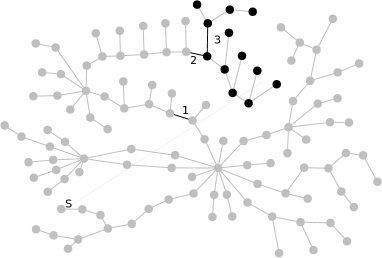
Fig. 3: Violations and upgrades for a part of the Zürich distribution grid with realistic upgrade data. Darker lines represent current violations.

Table 1: Upgrade results for 30-bus case

	No policy	OPF	Newton PF
Upgrades	None	None	1,2,3
Cost	0	0	3
Slack active power	No result	-35.8 MW	150 MW
Slack reactive power	No result	26.7 MVar	1.2 MVar
Average $|v|$ slack	No result	0.020 p.u.	0.014 p.u.

Table 2: Upgrade results for 116-bus case

	No policy	OPF	Newton PF
Upgrades	None	3	1,2,3
Cost	0	1	3
Slack active power	No result	3.19 MW	3.15 MW
Slack reactive power	No result	0.63 MVAr	0.64 MVAr
Average $|v|$ slack	No result	0.054 p.u.	0.050 p.u.

4.2 Case study: IEEE 30-bus network

As a first demonstration, consider the IEEE 30-bus system from MATPOWER [18]. Being far from radial, the guarantees for convexification are not guaranteed to hold. We use the existing load data from MATPOWER along with tightened voltage limits $[1.01,1.07]$ as a violating snapshot. For upgrades, each line was allowed to be upgraded to $1.5$ or $3$ times its original admittance, at constant ratio of conductance to susceptance.

Figure 2 shows the network and locations of violations and Table 1 shows the upgrades obtained for different policies. When the optimization was run, both the relaxed problem (15) as well as the problem with the AC OPF policy constraint (ii) required no upgrades. Re-dispatch from the AC OPF was sufficient to satisfy the tightened voltage constraints. Note that the re-dispatch of the AC OPF led to active power flowing out through the slack bus in the system – other generators were dispatched to generate more power in this case. For the Newton AC power flow policy (iii), upgrades were required: After an hour of optimization, the lower bound was raised to 2 upgrades, whereas the best solution found had 3 upgrades.

4.3 Case study: 116-bus network

This example studies part of the distribution grid in Zürich, Switzerland. This grid has 116 buses and is almost radial: One cycle of length 6 is present. Actual load data was used, enhanced with some fictional generation to simulate a large curtailable PV installation far away from the slack bus. The resulting data leads to a steady state that violates both the voltage bounds and some current bounds. Physically available line parameters were used for upgrade possibilities, for a total of 525 possible upgrades (locations and strengths were picked in a case study and discussion with the DSO).

Figure 3 shows this network and locations of violations and Table 2 shows the upgrades obtained. In this application, the solution of the problem without any operating policy is to not perform any upgrades. This is due to the SDP relaxation (15) being feasible for the operational constraints, despite OPF solvers not finding any feasible solutions. In this case, a system designer would not get much information from this result, since not upgrading the system is not an option. When the AC OPF policy constraint (i.e., policy (ii)) is added, a solution with one upgrade is found. This solution has the added benefit of a certificate that if the AC OPF operating policy is used in practice, the upgrades as found by the procedure are certified to work for the given load pattern. If policy (iii) is used, two additional upgrades are required for the operation since the policy does not optimize the power dispatch. The optimization with policy (ii) found a first solution with 4 upgrades within seconds, then took 10 minutes to improve that solution to one upgrade and close the gap. For policy (iii), a solution with 4 upgrades was also found quickly, but after an hour of runtime, the best solution found was 3 upgrades with a lower bound of 2.

4.4 Discussion

The addition of policy constraints opens many possibilities for better modeling of the real system and its operation. However, since there is no analytical information about the policy function $g(a,s)$, each policy cut inherently only removes one upgrade configuration from consideration. In other words, if a lot of policy cuts are required, the performance of the method approaches that of a brute force evaluation of all upgrade possibilities.

In the experiments, it was found that the AC OPF operating policy is rather good at finding feasible points if they exist — meaning the set $\mathcal{F}_{\eqref{eqn:upgradeproblem_cvx}}\setminus\mathcal{F}_{\eqref{eqn:upgradeproblem2}}$ was found to be small. However, the Newton power flow policy fared worse in this respect: Many policy cuts were required. It would therefore be advisable to include analytical information such as convex relaxations of $g(a,s)$ into Problem (15), if available.

The policy constraints can also be used to investigate trade-offs between upgrades to the system and policy changes. For example, it was found that if the PV installation in the 116-bus example is allowed to be further curtailed, fewer upgrades will be required. The base case in the experiment was a 20 curtailment. If no curtailment is allowed, the same upgrades as for the Newton power flow are required since the only dispatchable power is the slack bus. If curtailment is raised to 25 scenario.

5 Conclusion

The method presented in this work outlines a systematic way of using convex relaxations and heuristic methods, as well as operating policy constraints to find globally optimal solutions to practical power system line upgrade problems. The addition of the operating policy constraints both made the problem more realistic as well as circumventing the hardness of checking AC power flow feasibility. An industrial example with real world data was presented, illustrating the features of the problem and demonstrating the effectiveness of the approach.

References

- [1] R. Walling, R. Saint, R. Dugan, J. Burke, and L. Kojovic, “Summary of distributed resources impact on power delivery systems,” IEEE Trans. on Power Delivery, vol. 23, pp. 1636–1644, July 2008.
- [2] S. Merkli, A. Domahidi, J. Jerez, M. Morari, and R. S. Smith, “Fast AC Power Flow Optimization using Difference of Convex Functions Programming,” IEEE Trans. on Power Systems, vol. 33, pp. 363–372, 2018.
- [3] M. J. Rider, A. V. Garcia, and R. Romero, “Power system transmission network expansion planning using AC model,” IET Generation, Transmission Distribution, vol. 1, pp. 731–742, September 2007.
- [4] I. J. Ramirez-Rosado and J. L. Bernal-Agustin, “Genetic algorithms applied to the design of large power distribution systems,” IEEE Trans. on Power Systems, vol. 13, pp. 696–703, May 1998.
- [5] L. H. Macedo, C. V. Montes, J. F. Franco, M. J. Rider, and R. Romero, “An MILP Branch Flow Model for Concurrent AC Multistage Transmission Expansion and Reactive Power Planning with Security Constraints,” IET Generation, Transmission & Distribution, vol. 10, pp. 3023–3032, 2016.
- [6] R. A. Jabr, “Optimization of AC transmission system planning,” IEEE Trans. on Power Systems, vol. 28, no. 3, pp. 2779–2787, 2013.
- [7] D. Bienstock and A. Verma, “Strong NP-hardness of AC power flows feasibility,” arXiv:1512.07315, 2015.
- [8] K. Lehmann, A. Grastien, and P. V. Hentenryck, “AC-Feasibility on Tree Networks is NP-Hard,” IEEE Trans. on Power Systems, vol. 31, pp. 798–801, Jan 2016.
- [9] S. H. Low, “Convex Relaxation of Optimal Power Flow - Part I: Formulations and Equivalence,” IEEE Trans. on Control of Network Systems, vol. 1, pp. 15–27, March 2014.
- [10] S. Merkli, “A Mixed-Integer QCQP Formulation of AC Power System Upgrade Planning Problems.” arXiv:1710.09228, 2017.
- [11] S. H. Low, “Convex Relaxation of Optimal Power Flow - Part II: Exactness,” IEEE Trans. on Control of Network Systems, vol. 1, pp. 177–189, June 2014.
- [12] S. Donovan, “An improved mixed integer programming model for wind farm layout optimisation,” in Proceedings of the 41st annual conference of the Operations Research Society, pp. 143–151, 2006.
- [13] J. Bezanson, A. Edelman, S. Karpinski, and V. B. Shah, “Julia: A fresh approach to numerical computing,” SIAM Review, vol. 59, no. 1, pp. 65–98, 2017.
- [14] I. Dunning, J. Huchette, and M. Lubin, “JuMP: A Modeling Language for Mathematical Optimization,” SIAM Review, vol. 59, no. 2, pp. 295–320, 2017.
- [15] A. Wächter and L. T. Biegler, “On the implementation of an interior-point filter line-search algorithm for large-scale nonlinear programming,” Math. prog., vol. 106, no. 1, pp. 25–57, 2006.
- [16] ApS, The MOSEK C optimizer API manual Version 7.0, 2015.
- [17] R. A. Jabr, “Exploiting sparsity in SDP relaxations of the OPF problem,” IEEE Trans. on Power Systems, vol. 27, no. 2, pp. 1138–1139, 2012.
- [18] R. Zimmerman, C. Murillo-Sánchez, and R. Thomas, “MATPOWER: Steady-State Operations, Planning, and Analysis Tools for Power Systems Research and Education,” IEEE Trans. on Power Systems, vol. 26, pp. 12–19, Feb 2011.