Span error bound for weighted SVM with applications in hyperparameter selection

Abstract

Weighted SVM (or fuzzy SVM) is the most widely used SVM variant owning its effectiveness to the use of instance weights. Proper selection of the instance weights can lead to increased generalization performance. In this work, we extend the span error bound theory to weighted SVM and we introduce effective hyperparameter selection methods for the weighted SVM algorithm. The significance of the presented work is that enables the application of span bound and span-rule with weighted SVM. The span bound is an upper bound of the leave-one-out error that can be calculated using a single trained SVM model. This is important since leave-one-out error is an almost unbiased estimator of the test error. Similarly, the span-rule gives the actual value of the leave-one-out error. Thus, one can apply span bound and span-rule as computationally lightweight alternatives of leave-one-out procedure for hyperparameter selection. The main theoretical contributions are: (a) we prove the necessary and sufficient condition for the existence of the span of a support vector in weighted SVM; and (b) we prove the extension of span bound and span-rule to weighted SVM. We experimentally evaluate the span bound and the span-rule for hyperparameter selection and we compare them with other methods that are applicable to weighted SVM: the $K$-fold cross-validation and the ${\xi}-{\alpha}$ bound. Experiments on 14 benchmark data sets and data sets with importance scores for the training instances show that: (a) the condition for the existence of span in weighted SVM is satisfied almost always; (b) the span-rule is the most effective method for weighted SVM hyperparameter selection; (c) the span-rule is the best predictor of the test error in the mean square error sense; and (d) the span-rule is efficient and, for certain problems, it can be calculated faster than $K$-fold cross-validation.

Keywords: span error bound, span-rule, hyperparameter selection, weighted SVM

1 Introduction

Weighted SVM (or fuzzy SVM) uses importance weights, $C_{i}$, for each training instance, $({\mathbf{x}}_{i},y_{i})$, and is one of the most commonly used variants of the soft-margin SVM (Lin and Wang, 2002). The algorithm was initially proposed as a robust SVM-based alternative for problems with outliers (Lin and Wang, 2002, 2004; Wu and Srihari, 2004). The weights regularize the misclassification penalty and therefore alter the contribution of each instance in the final solution. Additionally, Lapin et al. (2014) showed that the instance weights of weighted SVM can express the same type of prior knowledge that can be encoded using privileged features, like the ones of the SVM+ algorithm (Vapnik and Vashist, 2009). The weighted SVM formulation is presented in detail in Section 2.1.

Weighted SVM can be applied on training instances with different importance or certainty. The different importance may be due to imbalanced or noisy classes, instances with feature noise (for example, measurement noise, outliers), instances with label noise (i.e. erroneous class label assignments), or instances with different importance (for example, importance scores assigned by an expert).

Weighted SVM applications have used instance weights to reflect: the importance of an instance using the class labels of its neighbors or its closest class cluster (Cheng et al., 2016; Wu et al., 2014); the class importance in problems with overlapping or imprecise label assignments (Hsu et al., 2009); or the density of the class around the training instance calculated with non-parametric methods (Bicego and Figueiredo, 2009). Also, the weights can be used to incorporate problem-specific knowledge for the individual importance of the training instances, for example: the score for bankruptcy in economics applications (Chaudhuri and De, 2011); the importance of the instances according to the user feedback in multimedia retrieval systems (Barrett et al., 2009); or the instance importance in automatically generated training sets from noisy sources, such as user clickthrough data harvested from search engine logs (Sarafis et al., 2015, 2016) or user-assigned tags (Papapanagiotou et al., 2015).

The selection of the SVM hyperparameters—including the regularization parameter $C$ for “standard” SVM (that is, without individual instance weights) and the individual instance weights $C_{i}$ for weighted SVM—is important in order to achieve good generalization performance. For standard SVM, various hyperparameter selection methods have been proposed and evaluated: ordinary $K$-fold cross-validation ($K$-fold CV) and leave-one-out procedure; genetic based methods (Huang and Wang, 2006); particle optimization methods (Lin et al., 2008); and generalized approximate cross-validation (Wahba et al., 1999).

In addition to the previous, upper bounds or estimators for the leave-one-out error aim to provide computationally cheaper alternatives of the actual leave-one-out procedure (Jaakkola and Haussler, 1999; Opper and Winther, 2000; Joachims, 2000). Vapnik and Chapelle (2000) introduced the concept of the span of a support vector which is a geometrical object defined using the support vectors of a trained SVM model. Based on the span, they proved the span bound, an upper bound of the leave-one-out error, for standard soft- and hard- margin SVM algorithms. Additionally, they proved the span-rule, a method that estimates the exact value of the leave-one-out error, and demonstrated its use for effective hyperparameter selection.

Although there are various leave-one-out error bounds and leave-one-out error prediction methods for standard soft- and hard- margin SVM, the existence of leave-one-out error estimators suitable for weighted SVM algorithm is fairly limited (Yang et al., 2015). The related work on leave-one-out error estimators and bounds for standard and weighted SVM is given in detail in Section 3.

1.1 Contribution of this work

This work extends the span error bound theory to weighted SVM algorithm. The new span bound and span-rule contribute both in theoretical understanding and in practical hyperparameter selection applications for this widely-used SVM variant.

More specifically, the key theoretical contributions of this work are:

• We prove in Lemma 1 the necessary and sufficient condition for the existence of the span of a support vector in a weighted SVM model. The importance of this lemma is that allows the extension of the span error bound theory to weighted SVM.

• We give in Theorem 1 the extension of the span bound (upper bound of the test error) to weighted SVM. The span bound takes into account both the support vectors that satisfy Lemma 1 and those that do not.

• We prove in Theorem 2 that, under the assumption that the support vectors do not change during the leave-one-out procedure, the condition of Lemma 1 is satisfied for all support vectors of a weighted SVM model. Also, Theorem 2 confirms the equality of Vapnik and Chapelle (2000) that is useful for identifying a support vector as a leave-one-out error.

• We confirm in Corollary 1 the extension of the span-rule of Vapnik and Chapelle (2000) to weighted SVM algorithm.

The experimental contributions verify the practical importance of the extended theory:

• We experimentally verify that the existence condition for the span of a support vector, given by Lemma 1, is satisfied almost always. This observation justifies the extension of the span error bound theory to weighted SVM algorithm and its usage in practical applications.

• We experimentally evaluate the effectiveness and efficiency of the span bound and the span-rule in comparison with other hyperparameter selection methods applicable to weighted SVM: the $K$-fold CV and the ${\xi\text{-}\alpha}$ bound of Yang et al. (2015).

• We compare the hyperparameter selection methods in two problems: (a) hyperparameter selection for class weights (that is, $C_{i}=C^{+}$ if $y_{i}=+1$ and $C_{i}=C^{-}$ if $y_{i}=-1$); and (b) hyperparameter selection to identify the optimal mapping from individual importance scores of the training instances, $q_{i}$, to individual instance weights, $C_{i}$.

• Effectiveness and efficiency experiments conducted on 14 standard benchmark data sets and data sets with instance importance scores demonstrate that: (a) the span-rule for weighted SVM is the best hyperparameter selection method in both examined problems; (b) the span-rule is the best predictor for the value of the actual testing error in the mean-square-error sense; and (c) the span-rule computation time is not only compelling but, in certain cases, it can be significantly faster than $K$-fold CV.

1.2 Organization

The rest of the paper is organized as follows. Section 2 briefly presents the preliminaries on weighted SVM formulation and the theorem for the unbiasedness of the leave-one-out error estimator. Then, Section 3 presents an overview of the related work on leave-one-out error bounds for SVM-based algorithms. Section 4 presents the span bound and span-rule for weighted SVM. Next, Section 5 illustrates the proposed hyperparameter selection approach using the span-rule. Finally, Section 6 presents the experimental analysis and Section 7 summarizes the findings and concludes the paper.

2 Preliminaries

This section briefly presents the preliminaries on weighted SVM (Section 2.1) and the theorem for the unbiasedness of the leave-one-out error estimator (Section 2.2).

2.1 The weighted SVM algorithm

Let ${T}_{l}$ be a training set of $l$ instances, ${T}_{l}=\{({\mathbf{x}}_{1},y_{1}),\dots,$ $({\mathbf{x}}_{l},y_{l})\}$, where ${\mathbf{x}}_{i}\in\mathbb{R}^{d}$ are the $d$-dimensional feature vectors and $y_{i}\in\{-1,+1\}$ are the class labels of the instances.

We consider the weighted SVM algorithm where a realization of the soft-margin separating hyperplane with threshold, ${\mathbf{w}}\cdot{\mathbf{x}}+b=0$, is computed from (Lin and Wang, 2002):

$$\min~{}\frac{1}{2}{\mathbf{w}}\cdot{\mathbf{w}} +\sum_{i=1}^{l}C_{i}\xi_{i}$$ (1)

$$s.t.~{}~{}y_{i}({\mathbf{w}}\cdot{\mathbf{x}}_{i}+b) \geq 1-\xi_{i},~{}~{}~{}i=1,\dots,l$$ (2)

$$\xi_{i} \geq 0,~{}~{}~{}i=1,\dots,l$$ (3)

The slack variables $\xi_{i}$ allow the training instances to violate the margin; a training instance violates the margin when $\xi_{i}>0$ and is misclassified when $\xi_{i}\geq 1$. The instance weights $C_{i}$ regularize the training error penalties in the objective function. A larger value for a $C_{i}$ makes more likely $\xi_{i}=0$ to occur.

The difference between the formulations of standard SVM and weighted SVM is that the latter uses the individual instance weights $C_{i}$ to regularize the effect of the training errors with a different intensity for each instance, whereas, for standard SVM it is $C_{i}=C$ for all training instances.

Equations (1), (2) and (3) define the primal problem of weighted SVM. The Lagrangian of the primal problem is:

$$\mathcal{L}_{P}=\frac{1}{2}{\mathbf{w}}\cdot{\mathbf{w}}+{\sum\limits_{i=1}^{l}}C_{i}\xi_{i}-{\sum\limits_{i=1}^{l}}{\alpha}_{i}[y_{i}({\mathbf{w}}\cdot{\mathbf{x}}_{i}+b)-1+\xi_{i}]-{\sum\limits_{i=1}^{l}}\mu_{i}\xi_{i}$$ (4)

where ${\alpha}_{i}$ and $\mu_{i}$ are the Lagrange multipliers from inequalities (2) and (3) respectively.

Taking the first order derivatives of $\mathcal{L}_{P}$ with respect to ${\mathbf{w}}$, $b$ and $\xi_{i}$, setting them to zero and substituting back to (4), leads to the dual problem for weighted SVM:

$$\max~{}W({\bm{\alpha}})\equiv{\sum\limits_{i=1}^{l}}{\alpha}_{i} -\frac{1}{2}{\sum\limits_{i,j=1}^{l}}{\alpha}_{i}{\alpha}_{j}y_{i}y_{j}{\mathbf{x}}_{i}\cdot{\mathbf{x}}_{j}$$ (5)

$$s.t.~{}~{}0\leq{\alpha}_{i} \leq C_{i}$$ (6)

$${\sum\limits_{i=1}^{l}}{\alpha}_{i}y_{i} =0$$ (7)

The Karush-Kuhn-Tucker (KKT) conditions for weighted SVM are:

$$\frac{\partial\mathcal{L}_{P}}{\partial{\mathbf{w}}}={\mathbf{w}}-{\sum\limits_{i=1}^{l}}{\alpha}_{i}y_{i}{\mathbf{x}}_{i} =0$$ (8)

$$\frac{\partial\mathcal{L}_{P}}{\partial b}=-{\sum\limits_{i=1}^{l}}{\alpha}_{i}y_{i} =0$$ (9)

$$\frac{\partial\mathcal{L}_{P}}{\partial\xi_{i}}=C_{i}-{\alpha}_{i}-\mu_{i} =0$$ (10)

$$y_{i}({\mathbf{w}}\cdot{\mathbf{x}}_{i}+b)-1+\xi_{i} \geq 0$$ (11)

$$\xi_{i} \geq 0$$ (12)

$${\alpha}_{i} \geq 0$$ (13)

$$\mu_{i} \geq 0$$ (14)

$${\alpha}_{i}\{y_{i}({\mathbf{w}}\cdot{\mathbf{x}}_{i}+b)-1+\xi_{i}\} =0$$ (15)

$$\mu_{i}\xi_{i} =0$$ (16)

Equations (15) and (16) represent the KKT complementary slackness conditions.

For a support vector with $0<{\alpha}_{i}<C_{i}$, equations (10) and (16) result to $\xi_{i}=0$. Also, from the same equations follows that when a support vector violates the margin ($\xi_{i}>0$) then ${\alpha}_{i}=C_{i}$.

We will use the notation of Vapnik and Chapelle (2000) to discriminate the categories of the support vectors. The instances of the training set will be sorted so that the first $n^{*}$ are the in-bound support vectors ($0<{\alpha}_{i}<C_{i}$) followed by the $m=n-n^{*}$ bounded support vectors (${\alpha}_{i}=C_{i}$). We consider only stable solutions where $n^{*}>0$; an assumption that generally holds true (Crisp and Burges, 1999).

There is no difference between weighted SVM and standard SVM for predicting the label of a new instance. That is, a new observation ${\mathbf{x}}$ is classified according to the sign of

$$f({\mathbf{x}})={\mathbf{w}}\cdot{\mathbf{x}}+b={\sum\limits_{i=1}^{l}}{\alpha}_{i}y_{i}{\mathbf{x}}_{i}\cdot{\mathbf{x}}+b$$ (17)

SVMs can be extended to produce non-linear solutions via the kernel trick, $K({\mathbf{x}},{\mathbf{x}}^{\prime})=\phi({\mathbf{x}})\cdot\phi({\mathbf{x}}^{\prime})$, where $\phi:\mathbb{R}^{d}\mapsto\mathcal{H}$ produces a mapping of the initial feature vectors to a higher dimensional space, $\mathcal{H}$. Section 4 will assume the linear kernel, $K({\mathbf{x}},{\mathbf{x}}^{\prime})={\mathbf{x}}\cdot{\mathbf{x}}^{\prime}$; however, the presented theory can be directly extended to non-linear SVMs.

2.2 The leave-one-out error theorem

In the problem of learning from examples, the learning machine is supplied with a training set of $l$ instances, ${T}_{l}=\{({\mathbf{x}}_{1},y_{1}),\dots,$ $({\mathbf{x}}_{l},y_{l})\}$, drawn i.i.d. from an unknown underlying joint distribution $F({\mathbf{x}},y)=F({\mathbf{x}})F(y|{\mathbf{x}})$.

Let us denote with $R(f_{T_{l}})$ the test error rate of a machine, $f$, trained on a sample $T_{l}$. One can use the $l$ instances of ${T}_{l}$ to calculate an estimate of $R(f_{T_{l}})$ through a leave-one-out procedure. In the leave-one-out procedure, one instance $({\mathbf{x}}_{i},y_{i})$ is omitted from the training set, a decision function is trained using the remaining $l-1$ instances and the error on the left-out instance is calculated. The procedure is repeated for each instance of the training set and the total number of errors is calculated.

Let $\mathcal{L}({\mathbf{x}}_{1},y_{1},\dots,{\mathbf{x}}_{l},y_{l})$ be the total number of errors from the leave-out-procedure on $T_{l}$. The leave-one-out error ${R_{\text{\tiny LOO}}}({T}_{l})$ is given by

$${R_{\text{\tiny LOO}}}({T}_{l})=\frac{1}{l}\mathcal{L}({\mathbf{x}}_{1},y_{1},\dots,{\mathbf{x}}_{l},y_{l})$$ (18)

The leave-one-out error is an almost unbiased estimator of the test error (Vapnik, 1998; Luntz and Brailovsky, 1969), that is:

$$E_{{T}_{l}}[{R_{\text{\tiny LOO}}}({T}_{l})]=E_{{T}_{l-1}}[R(f_{T_{l-1}})]$$ (19)

where the expectation $E_{{T}_{l}}[{R_{\text{\tiny LOO}}}({T}_{l})]$ is taken over the ensemble of training sets of size $l$ and $E_{{T}_{l-1}}[R(f_{T_{l-1}})]$ is the expectation of the test error for the learning machine trained on $l-1$ instances. The “almost” refers to the fact that the test error estimated by leave-one-out procedure is for the learning machine trained on sets of size $l-1$ instead of $l$.

The leave-one-out theorem (eq. 19) is the basis of the examined error bounds and error estimators presented next.

3 Related Work

This section gives an overview of the leave-one-out error bounds and leave-one-out error estimators for SVM-based algorithms.

Although the leave-one-out error is an almost unbiased estimator of the test error, its actual calculation is generally impractical due to high computational cost. To this end, a number of approximations or upper bounds have been proposed that attempt to estimate the leave-one-out error using only a single SVM model that is trained with all available instances of the training set ${T}_{l}$. Using these methods we do not need to train additional SVM models; whereas, this is required by other hyperparameter selection methods (such as, the $K$-fold CV).

A training instance that is not a support vector is correctly classified by the SVM model. Also, since the SVM solution is unique, removing from ${T}_{l}$ a training instance that is not support vector leaves the hyperplane unchanged. Thus, the number of support vectors, $n$, is an upper bound of the leave-one-out errors (Vapnik, 1998),

$${R_{\text{\tiny LOO}}}({T}_{l})\leq\frac{n}{l}$$ (20)

For the separable case and hard-margin SVM without threshold (that is, separating hyperplanes in the form: ${\mathbf{w}}\cdot{\mathbf{x}}=0$), Vapnik (1998) proved the radius-margin bound

$${R_{\text{\tiny LOO}}}({T}_{l})\leq\frac{1}{4l}D^{2}||{\mathbf{w}}||^{2}$$

where $D$ is the diameter of the smallest sphere containing the training set.

Chapelle et al. (2002) calculated the gradient of the radius-margin bound and showed that it can be used for SVM parameter tuning and feature selection via gradient descent methods over the parameter set.

A modified version of radius-margin bound for soft-margin SVM was studied by Duan et al. (2003) and showed adequate performance for the problem of hyperparameter selection. A version of radius-margin bound for $L_{2}$ soft-margin SVM was proposed by Keerthi (2002).

For hard-margin SVM, Jaakkola and Haussler (1999) used probabilistic regression models to prove an upper bound of the leave-one-out error

$${R_{\text{\tiny LOO}}}({T}_{l})\leq\frac{1}{l}\sum\limits_{p=1}^{l}\theta\left(y_{p}[f({\mathbf{x}}_{p})-{\alpha}_{p}K({\mathbf{x}}_{p},{\mathbf{x}}_{p})]\right)$$

where ${\alpha}_{p}$ are the Lagrange multipliers of the support vectors, $\theta$ is the step function ($\theta(t)=1\text{ when }t\geq 0\text{ and }\theta(t)=0\text{ otherwise}$), $K({\mathbf{x}},{\mathbf{x}}^{\prime})$ is the kernel function and $f({\mathbf{x}})$ is the decision function.

Opper and Winther (2000) proposed an approximation of the leave-one-out error based on methods from statistical physics. Under the assumption that the set of in-bound and the set of bounded support vectors do not change during leave-one-out procedure, an estimate of the leave-one-out error is given by

$$t_{l}=\frac{1}{l}\sum\limits_{p=1}^{l}\theta\left(\frac{a_{p}}{(\mathbf{K}_{SV}^{-1})_{pp}}-1\right)$$

where $\mathbf{K}_{SV}$ is the Gram matrix of the support vectors.

Similar to the Jaakkola-Haussler bound, the ${\xi\text{-}\alpha}$ bound for the soft-margin SVM algorithm with threshold was proposed by Joachims (2000). This bound is calculated using the Lagrange multipliers of the support vectors, ${\alpha}_{p}$, and the slack variables $\xi_{p}$. Although ${\xi\text{-}\alpha}$ bound is fairly conservative it was effectively used for hyperparameter selection with SVM-based text classifiers.

Yang et al. (2015) showed that the ${\xi\text{-}\alpha}$ bound can be applied to weighted SVM as well. For the weighted SVM formulation of Section 2.1, the ${\xi\text{-}\alpha}$ error bound is given by

$${R_{\text{\tiny LOO}}}({T}_{l})\leq\frac{1}{l}\sum\limits_{p=1}^{l}\theta\left(2{\alpha}_{p}R_{\Delta}^{2}+\xi_{p}-1\right)$$ (21)

where $R_{\Delta}^{2}$ satisfies $c\leq K({\mathbf{x}}_{i},{\mathbf{x}}_{j})\leq c+R_{\Delta}^{2}$ for all ${\mathbf{x}}_{i},{\mathbf{x}}_{j}$ and a constant $c$.

Note that the ${\xi\text{-}\alpha}$ bound is the only leave-one-out error bound in the literature that can be applied with weighted SVM. To this end, the bound of (21) is experimentally evaluated in this work for comparison purposes.

Vapnik and Chapelle (2000); Chapelle and Vapnik (2000) introduced the concept of the span of a support vector—a geometrical object defined using the remaining in-bound support vectors of the SVM solution when a support vector is left out—and used it to derive the span bound and the span-rule. The concept of the span and its calculation will be described in detail in Section 4.

If $S_{p}$ is the distance of the $p$-th left-out support vector, ${\mathbf{x}}_{p}$, from the corresponding geometrical object then the span bound is given by

$${R_{\text{\tiny LOO}}}({T}_{l})\leq\frac{S\sum_{p=1}^{n^{*}}[\max(D,1/\sqrt{C}){\alpha}_{p}^{0}]+m}{l}$$ (22)

where $S=\max_{\begin{subarray}{c}p=1,\dots,n^{*}\end{subarray}}S_{p}$ and $n^{*}$ is the number of in-bound support vectors.

Also, under the assumption that the sets of in-bound and bounded support vectors do not change in leave-one-out procedure, the span-rule calculated by

$$t_{l}=\frac{1}{l}\sum\limits_{p=1}^{l}\theta\left({\alpha}_{p}S_{p}^{2}-y_{p}f({\mathbf{x}}_{p})\right)$$ (23)

gives the exact value of the leave-one-out error; that is, ${R_{\text{\tiny LOO}}}({T}_{l})=t_{l}$.

The intuition behind span bound and span-rule is that smaller distance, $S_{p}$, and smaller Lagrange multiplier, ${\alpha}_{p}$, indicate that the support vector is less likely to be a leave-one-out error.

Additionally, it was shown that the value of $S_{p}$ is smaller than the diameter of the sphere that encloses the in-bound support vectors and, for this reason, the span-rule is considered to give accurate error estimates (Vapnik and Chapelle, 2000; Duan et al., 2003; Schölkopf and Smola, 2002). Regarding the efficiency, it was shown that the use of span-rule can be significantly faster than executing an actual leave-one-out procedure.

In this work, we prove the necessary and sufficient condition for the existence of the span of a support vector in a weighted SVM solution (in Lemma 1) and we show that the span bound and the span-rule can be defined for weighted SVM as well (in Theorems 1 and 2 respectively). Extensive experimental analysis shows that the span-rule is an effective and efficient hyperparameter selection method for the weighted SVM algorithm.

4 Span Bound and Span-Rule for Weighted SVM

This section presents the extension of the span error bound theory to weighted SVM. First, in Section 4.1 we define the span of a support vector for weighted SVM. Most importantly, we provide in Lemma 1 the non-trivial proof for the necessary and sufficient condition for the existence of the span of a support vector in a weighted SVM model. Then, in Section 4.2 we extend the span bound to weighted SVM.

Next, in Section 4.3 we give in Corollary 1 the span-rule for weighted SVM. Notably, we prove in Theorem 2 that, under the assumption that the support vectors do not change during leave-one-out procedure, the value of the span can be calculated for any support vector; that is, the existence condition of Lemma 1 is always satisfied. Thus, the span-rule for weighted SVM is applied using all the support vectors, similar to the span-rule for standard SVM.

4.1 Span of a support vector in weighted SVM

Let us consider that the instances of the training set ${T}_{l}$ are ordered so that the first $n$ ones are the support vectors, $({\mathbf{x}}_{1},y_{1}),\dots,({\mathbf{x}}_{n},y_{n})$. Also, let ${\bm{\alpha}}^{0}=({\alpha}_{1}^{0},\dots,{\alpha}_{n}^{0},0,\dots,0)$ be the vector of the Lagrange multipliers for the weighted SVM solution trained on the initial training set (that is, using all instances of ${T}_{l}$).

We consider that the supports vectors are also ordered, so that the first $n^{*}$ are the in-bound support vectors ($0<{\alpha}_{i}^{0}<C_{i},~{}i=1,\dots,n^{*}$) and the remaining $m=n-n^{*}$ are the bounded support vectors (${\alpha}_{i}^{0}=C_{i},~{}i=n^{*}+1,\dots,n$).

The in-bound support vectors are used for defining the set ${\Lambda_{p}}$. For an in-bound support vector ${\mathbf{x}}_{p}$, we define the set ${\Lambda_{p}}$ using the remaining in-bound support vectors as:

$$\Lambda_{p}=\Bigg{\{}{\sum\limits_{i=1,i\neq p}^{n^{*}}}{\lambda}_{i}{\mathbf{x}}_{i}:{\sum\limits_{i=1,i\neq p}^{n^{*}}}{\lambda}_{i}=1,\text{and }0\leq{\alpha}^{0}_{i}+y_{i}y_{p}{\alpha}^{0}_{p}{\lambda}_{i}\leq C_{i}~{}~{}\forall i=1,\dots,n^{*},~{}i\neq p\Bigg{\}}$$ (24)

where ${\lambda}_{i}$ are real-valued variables.

The set ${\Lambda_{p}}$ is the basis of the span error bound theory for weighted SVM. We can acquire the corresponding set for standard SVM by setting $C_{i}=C$.

For the standard SVM, it was shown by Vapnik and Chapelle (2000) that the set ${\Lambda_{p}}$ is non-empty for all support vectors. However, as we will prove next, this is not true for the weighted SVM algorithm. Thus, in order to extend the span error bound theory to weighted SVM we need to examine when the set ${\Lambda_{p}}$ can be defined (that is, the conditions assuring that ${\Lambda_{p}}\neq\emptyset$).

The following lemma provides the necessary and sufficient condition for the existence of ${\Lambda_{p}}$ which is needed to extend the span error bound theory to weighted SVM.

Lemma 1 The set ${\Lambda_{p}}$ for a fixed in-bound support vector ${\mathbf{x}}_{p}$ of a weighted SVM solution is non-empty if and only if

$${\sum\limits_{\begin{subarray}{c}i=1,i\neq p,\\ y_{i}=y_{p}\end{subarray}}^{n^{*}}}C_{i}+y_{p}{\sum\limits_{i=n^{*}+1}^{n}}y_{i}C_{i}\geq 0$$ (25)

 

Proof is in Appendix A.1.

The importance of Lemma 1 lies on the fact that without it we would not be able to extend the span error bound theory to weighted SVM algorithm.

For weighted SVM we define the span $S_{p}$ of a support vector ${\mathbf{x}}_{p}$ as its distance from the set ${\Lambda_{p}}$ when the set is non-empty,

$$S_{p}^{2}=d^{2}({\mathbf{x}}_{p},{\Lambda_{p}})=\min_{{\mathbf{x}}\in{\Lambda_{p}}}({\mathbf{x}}-{\mathbf{x}}_{p})^{2},~{}~{}{\Lambda_{p}}\neq\emptyset$$ (26)

The support vector ${\mathbf{x}}_{p}$ in (26) can be in-bound or bounded.

If the necessary and sufficient condition of Lemma 1 does not hold for an in-bound support vector ${\mathbf{x}}_{p}$ then we consider that the value of $S_{p}$ cannot be calculated for this support vector. Nevertheless, experimental analysis of weighted SVM models on various data sets shows that the occurrence of ${\Lambda_{p}}=\emptyset$ is a very rare exception (see Section 6.5).

The property of standard SVM for the span

$$S_{p}\leq D_{SV}$$ (27)

holds for weighted SVM as well (see remark of proof, Appendix A.1). $D_{SV}$ is the diameter of the smallest sphere enclosing the in-bound support vectors.

Using (24), (26), setting ${\lambda}_{p}=-1$ and ${\lambda}_{i}=0\text{ for }i>n^{*}\text{, }i\neq p~{}$ we can calculate the value of $S_{p}^{2}$ for any support vector from the following:

$$S_{p}^{2}\equiv\min_{{\lambda}_{i}}\left({\sum\limits_{i=1}^{n}}{\lambda}_{i}{\mathbf{x}}_{i}\right)^{2}$$ (28)

s.t. $${\lambda}_{p}=-1$$ (29)

$${\sum\limits_{i=1}^{n}}{\lambda}_{i}=0$$ (30)

$$0\leq{\alpha}^{0}_{i}+y_{i}y_{p}{\alpha}^{0}_{p}{\lambda}_{i}\leq C_{i},~{}~{}~{}\forall i\neq p$$ (31)

$${\lambda}_{i}=0,~{}~{}~{}\forall i>n^{*}\text{ and }i\neq p$$ (32)

As we will see later, under the assumption that the support vectors do not change during leave-one-out procedure, the box constrains of (31) may be dropped.

Finally, we define the $S$-span for weighted SVM as the maximum value of $S_{p}$ among the in-bound support vectors with ${\Lambda_{p}}\neq\emptyset$,

$$S=\max_{\begin{subarray}{c}p=1,\dots,n^{*}\\ {\Lambda_{p}}\neq\emptyset\end{subarray}}S_{p}$$ (33)

4.2 Span bound for weighted SVM

In this section, we present the extension of the span bound to weighted SVM. We begin with the following lemma:

Lemma 2 If in the leave-one-out procedure an in-bound support vector ($0<{\alpha}_{p}^{0}<C_{p},~{}~{}p=1,\dots,n^{*}$) with ${\Lambda_{p}}\neq\emptyset$ is misclassified, then the inequality

$${\alpha}_{p}^{0}S_{p}\max\left(D,\frac{1}{\sqrt{C_{p}}}\right)\geq 1$$

holds true. $D$ is the diameter of the smallest sphere enclosing the training set.  

This proof is omitted due to similarity with the corresponding proof for standard SVM in the non-separable case (see Lemma 2.3 of Vapnik and Chapelle, 2000). The only differences in executing the proof of this lemma originate from the individual instance weights $C_{i}$.

Let us denote with $k$ the number of in-bound support vectors where the condition of Lemma 1 is not satisfied and, thus, for these support vectors it is ${\Lambda_{p}}=\emptyset$. Also, suppose that the in-bound support vectors are further ordered so that the first $n^{*}-k$ in-bound support vectors are the ones with ${\Lambda_{p}}\neq\emptyset$.

Using Lemma 1 and Lemma 2 we can prove the span bound theorem for the expectation of the test error for weighted SVM.

Theorem 1 The expectation of the test error $E_{{T}_{l-1}}[R({\alpha}^{(l-1)})]$ for a weighted SVM model trained on $l-1$ instances has the bound

$$E_{{T}_{l-1}}[R({\alpha}^{(l-1)})]\leq E_{{T}_{l}}\left[\frac{S\sum_{p=1}^{n^{*}-k}[\max(D,1/\sqrt{C_{p}}){\alpha}_{p}^{0}]+k+m}{l}\right]$$

where $n^{*}-k$ is the number of in-bound support vectors that satisfy the inequality of Lemma 1 (that is, the support vectors with ${\Lambda_{p}}\neq\emptyset$), $k$ is the number of the in-bound support vectors where the inequality of Lemma 1 is not satisfied (that is, the support vectors with ${\Lambda_{p}}=\emptyset$), and $m=n-n^{*}$ is the number of the bounded support vectors. The values, $S,$ of S-span, the diameter, $D,$ of the sphere containing the training set and the Lagrange multipliers, ${\alpha}_{p}^{0}$, of the weighted SVM model are considered for training set of size $l$.  

Proof is in Appendix A.2.

Theorem 1 can be viewed as an extension of the original span bound. Indeed, since for standard SVM it is always $k=0$, we can acquire the span bound for the non-separable case of standard SVM.

Because the $k$ in-bound support vectors with ${\Lambda_{p}}=\emptyset$ are counted as leave-one-out errors, the error bound of Theorem 1 appears to be less tight when applied to weighted SVM than standard SVM. More specifically, if the equation of Lemma 1 is not satisfied for any of the in-bound support vectors (that is, if $k=n^{*}$), then the error bound becomes

$$E_{{T}_{l-1}}[R({\alpha}^{(l-1)})]\leq E_{{T}_{l-1}}\left[\frac{n^{*}+m}{l}\right]=E_{{T}_{l-1}}\left[\frac{n}{l}\right]$$ (34)

Thus, in this case, the span bound degenerates to the support-vector-count error bound given by (20). Nevertheless, the experimental results show that the occurrence of ${\Lambda_{p}}=\emptyset$ is very rare and the error bound of Theorem 1 is virtually unaffected by these support vectors.

4.3 Span-rule for weighted SVM

The bound defined by Theorem 1 is always available, however, by posing realistic assumptions we can reach an exact estimate of the test error instead of an error bound.

The span-rule, presented next, gives the value of the leave-one-out error under the assumption that the support vectors do not change during the leave-one-out procedure (Vapnik and Chapelle, 2000). The same assumption was made in deriving the bounds of Opper and Winther (2000).

We begin by proving the following theorem for weighted SVM:

Theorem 2 Under the assumption that the sets of the in-bound and bounded support vectors remain the same during the leave-one-out-procedure, then for any support vector ${\mathbf{x}}_{p}$ the inequality of Lemma 1 is always satisfied and ${\Lambda_{p}}\neq\emptyset$. Furthermore, for any support vector, the following equality holds true:

$$y_{p}(f^{0}({\mathbf{x}}_{p})-f^{p}({\mathbf{x}}_{p}))={\alpha}_{p}^{0}S_{p}^{2}$$ (35)

where $f^{0}$ and $f^{p}$ are the decision functions for the weighted SVM trained on the whole training set and the training set after the removal of ${\mathbf{x}}_{p}$ respectively.  

Proof is in Appendix A.3.

Theorem 2 denotes that, under the assumption that the support vectors do not change during leave-one-out procedure, the inequality of Lemma 1 is always satisfied. This is an important finding since the theorem’s assumption is generally true for most of the support vectors. Theorem 2 also aligns with the experimental observation that the inequality of Lemma 1 is satisfied almost always (see Section 6.5).

Similarly to the corresponding theorem for standard SVM, other gains of Theorem 2 compared to Theorem 1 are: (a) the inequality becomes an equality, (b) the value $D$ diminishes and instead the smaller value of $S_{p}$ appears in the equation; (c) the theorem can be applied for all support vectors; and (d) the box constrains of (24) are trivially satisfied and can be dropped from the calculation of $S_{p}$ (as shown in first part of theorem’s proof).

From the equality (35) we deduce that a leave-one-out error (that is, $y_{p}f^{p}({\mathbf{x}}_{p})\leq 0$) will occur for support vector ${\mathbf{x}}_{p}$ when

$${\alpha}_{p}^{0}S_{p}^{2}\geq y_{p}f^{0}({\mathbf{x}}_{p}),~{}~{}p=1,\dots,n$$ (36)

Using the leave-one-out theorem (eq. 19) and taking into account inequality (36) we get the span-rule for weighted SVM.

Corollary 1 – Span-rule Under the assumption of Theorem 2, the leave-one-out error, ${R_{\text{\tiny LOO}}}$, is equal to

$$t_{l}\equiv\frac{1}{l}\sum\limits_{p=1}^{n}\theta\left({\alpha}_{p}^{0}S_{p}^{2}-y_{p}f^{0}({\mathbf{x}}_{p})\right)$$ (37)

where $\theta$ is the step function; $\theta(t)=1\text{ when }t\geq 0\text{ and }\theta(t)=0\text{ otherwise}$.

The span-rule of Corollary 1 is applied using all support vectors since Theorem 2 guarantees the existence of the span, $S_{p}$, for all support vectors under the theorem’s assumption.

Note that, contrary to the actual leave-one-out procedure, the computation of $t_{l}$ requires training only one weighted SVM model; however, we do need to compute $n$ different values of $S_{p}$. Sections 6.6 and 6.7 examine when this is computationally attractive.

We can apply the span-rule in the following practical problems:

• Given a trained weighted SVM model, we can estimate the value of the testing error.

• Most importantly, we can use the span-rule as a typical hyperparameter selection tool. That is, we can train weighted SVM models with different parameterizations (for example, different weights $C_{i}$) and select the model with the best generalization performance. Next section sketches the proposed approach for weighted SVM hyperparameter selection using the span-rule.

5 Hyperparameter selection using the span-rule

The goal of hyperparameter selection (or model selection) is to discover the training hyperparameters that yield the model with the best generalization performance; that is, the model that will be able to classify unknown instances with the smallest classification error.

This work enables a new method to perform hyperparameter selection for weighted SVM that was not previously possible. A sketch of the proposed method for instance weights selection is illustrated in Figure 1.

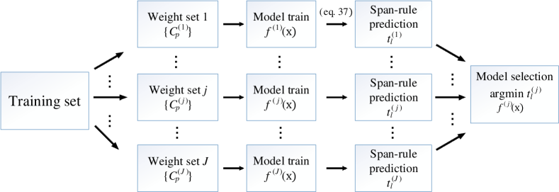
Figure 1: Sketch of the proposed approach for hyperparameter selection. Each one of the $J$ branches produces a final, weighted SVM model with an estimation of its test error.

At $j$-th iteration, we execute the following three steps:

1. Generation of training hyperparameters. A set of instance weights, $\{C^{(j)}_{p},~{}p=1,\dots,l\}$, is generated. Also, other training hyperparameters may be set, such as the kernel-specific parameters for non-linear SVMs.

2. Weighted SVM model training. A weighted SVM model with decision function $f^{(j)}({\mathbf{x}})$ is trained using all available training instances and the weights generated in the previous step.

3. Test error prediction using span-rule. Using the span-rule, the error prediction, $t_{l}^{(j)}$, is calculated for the $j$-th candidate weighted SVM model.

We repeat these steps for a total of $J$ parameterizations. In the end, $J$ candidate weighted SVM models with decision functions $f^{(j)}({\mathbf{x}})$ are available and each model is accompanied with a prediction for the testing error of the model. This prediction reflects an assessment of its generalization performance.

The final step is to select the model with the best performance according to

$$\operatorname*{argmin}\limits_{\begin{subarray}{c}f^{(j)}({\mathbf{x}})\end{subarray}}t^{(j)}_{l},~{}~{}~{}j=1,\dots,J$$ (38)

Although other hyperparameter selection methods can be used for test error estimation in the place of span-rule in step 3, the experiments demonstrate that the span-rule is the most effective and, in certain cases, the most efficient method for the weighted SVM algorithm.

6 Experiments

This section presents the experimental analysis and is organized as follows:

• Section 6.1 gives an overview of the data sets. Two types of data sets are used: (a) standard benchmark data sets; (b) data sets where a problem-specific, importance score $q_{i}$ is known for each training instance.

• Section 6.2 (Experiment #1) presents the experimental evaluation of the span bound of Theorem 1 and the span-rule of Corollary 1 on the task of selecting optimal class weights $C^{+}/C^{-}$. The standard benchmark data sets are used. The methods are compared to other hyperparameter selection methods applicable to weighted SVM: the $K$-fold CV (with $K=5$, which is a fairly common choice) and the ${\xi\text{-}\alpha}$ bound for weighted SVM.

• Section 6.3 (Experiment #2) presents the evaluation of the four examined hyperparameter selection methods on the task of selecting optimal, individual instance weights $C_{i}$ using the importance enconded in the scores $q_{i}$. The data sets with problem-specific importance scores assigned for each training instance are used.

• Section 6.4 (Experiment #3) presents the evaluation of the span-rule, $K$-fold CV and the ${\xi\text{-}\alpha}$ bound on the task of predicting the actual value of the test error. Both types of data sets are used for this evaluation.

• Section 6.5 (Experiment #4) presents an experimental investigation on the satisfaction of the inequality of Lemma 1 that guarantees the non-emptiness of the set ${\Lambda_{p}}$ and, consequently, the existence of the span, $S_{p}$. Both types of data sets are used.

• Section 6.6 (Experiment #5) presents the efficiency evaluation of the two most prominent methods: the span-rule and the $K$-fold CV. Both types of data sets are used.

• Section 6.7 (Experiment #6) aims to answer when it is faster to use span-rule than $K$-fold CV through experiments on synthetic data with varying training set sizes and feature dimensionality.

• Section 6.8 summarizes the most important experimental findings.

Implementation details.

We use LibSVM (Chang and Lin, 2011) for training the weighted SVM models and executing the $K$-fold CV. The default cache size of $100$MB is used. The MOSEK optimizer (MOSEK ApS, 2017) is used for calculating the value of the span $S_{p}$ by solving (28)-(32). Under the assumption of Theorem 2, we can drop the box constrains (eq. 31) for the calculation of $S_{p}$ for span-rule (as shown in first part of theorem’s proof, Appendix A.3). Finally, the implementation of ${\xi\text{-}\alpha}$ bound of (21) is fairly simple as it can be calculated directly from the trained SVM models.

6.1 Data sets

Table 1 displays an overview of the data sets. Following the suggestion of Duan et al. (2003), we use large testing sets in order to achieve accurate assessments of the generalization performance. In this section, we will refer to the error rate on the testing sets as “test error”. Two types of data sets are used: standard benchmark data sets and data sets with problem-specific knowledge for the instances’ importance.

	Training set	Testing set	Feature
Data set	size	size	size
breast cancer	$100$	$783$	$10$
mushrooms	$200$	$7924$	$112$
waveform	$400$	$4600$	$21$
banana	$400$	$4900$	$2$
skin nonskin	$500$	$244\,557$	$3$
splice	$1000$	$2175$	$60$
image	$1300$	$1010$	$18$
adult	$1605$	$30\,956$	$123$
MNIST 2’s vs. 9’s	$11\,907$	$2041$	$780$
MNIST 1’s vs. 7’s	$13\,007$	$2163$	$780$
MNIST 3’s vs. 6’s	$12\,049$	$1968$	$780$
MNIST 0’s vs. 8’s	$11\,774$	$1954$	$780$
Parkinson’s speech	$520$	$520$	$26$
bank marketing	$300$	$40\,888$	$11$

Table 1: Overview of the data sets.

6.1.1 Benchmark data sets

These are commonly-used benchmark data sets from various repositories: breast cancer, mushrooms, waveform, banana, skin nonskin, splice, image and adult (Lichman, 2013; IDA, ; Delve, ). Also, we use the MNIST data set (Lecun et al., 1998) to generate four binary classification problems: 2’s vs. 9’s; 1’s vs. 7’s; 3’s vs. 6’s; and 0’s vs. 8’s.

6.1.2 Data sets with importance scores for training instances

Apart from the standard benchmark data sets, we use two data sets that provide additional information for assigning the individual importance of each training instance. These data sets are:

• Parkinson’s speech data set. The data set is provided by Sakar et al. (2013). The instances consist of 26 features extracted using multiple types of sound recordings collected by 20 healthy and 20 PWP (People with Parkinson’s disease) individuals. Using this data set we build binary models to predict if a new measurement is from a healthy or PWP individual.

  Each of the 40 individuals in the provided training set has 26 recordings; a total of 1040 recordings is given. Because the provided testing set consists of 168 recordings only from PWP individuals, we modified the training/testing set splits for our experiments. The individuals are split into training and testing sets so that each set has measurements originating from 10 healthy and 10 PWP individuals. The training set contains the individuals with IDs: 1–10, 21–30; the testing set contains the individuals with IDs: 11–20 and 31–40.

  Also, the data set provides the UPDRS (Unified Parkinson’s disease rating scale) score for each PWP individual. The UPDRS score is an indication for the severity of the disease and it is determined by an expert via interview and clinical observation (Goetz et al., 2008). In Experiment #2, we will use the UPDRS score to generate instance weights $C_{i}$.

• Bank marketing data set. The data set is provided by Moro et al. (2014). It contains data of phone call marketing campaigns from a Portuguese banking institution. The data set consists of $41188$ instances. In our experiments, we use the following numerical features: age, previous numbers of calls, employment variation rate, consumer price index, consumer confidence index, euribor 3 month rate, number of employees; and the following boolean features: “has credit in default?”, “has housing loan?”, “has personal loan?”, “is married?”. The class of the instances is whether a client subscribed to the product of the campaign or not.

  The data set also provides the duration of the phone calls. The goal is to generate the models that predict the outcome of the phone call before it is actually made, thus, since the phone call duration is not known beforehand, it should not be used as a feature (Moro et al., 2014). Nevertheless, we will take advantage of this information in Experiment #2 to generate instance weights, $C_{i}$, for weighted SVM training.

6.2 Experiment #1: Selecting optimal class weights $C^{+}/C^{-}$

A very common application of weighted SVM is the use of class weights that alter the contribution of each class to the training error. That is, the weights are assigned as: $C_{i}=C^{+}$ if $y_{i}=+1$ and $C_{i}=C^{-}$ if $y_{i}=-1$. In fact, this weighting scheme is so common that most SVM solver libraries provide it as part of the “standard” SVM functionality.

Following the hyperparameter selection paradigm described in Section 5, we execute a grid search for the optimal training parameters for the values of $C^{+}$ and $C^{-}$. The parameters $C^{+}$ and $C^{-}$ are taking values from $log_{2}C^{\pm}=-6$ to $log_{2}C^{\pm}=+10$ with logarithmic step $0.5$. This grid search results to $J=1089$ weighted SVM models for each data set.

Data set		Span-rule	Span bound	$K$-fold CV	${\xi\text{-}\alpha}$ bound		Min. error
breast cancer		0.0360	0.0395	0.0377	0.0360		0.0292
mushrooms		0.0151	0.0154	0.0456	0.0623		0.0133
waveform		0.1141	0.1226	0.1104	0.1422		0.1052
banana		0.2324	0.4476	0.2324	0.4476		0.2324
skin nonskin		0.0086	0.0143	0.0131	0.0104		0.0061
splice		0.1080	0.1237	0.1085	0.1591		0.1016
image		0.0623	0.1158	0.0623	0.0852		0.0623
adult		0.1585	0.2405	0.1628	0.2405		0.1557
MNIST 2’s vs. 9’s		0.0049	0.0103	0.0059	0.0103		0.0049
MNIST 1’s vs. 7’s		0.0042	0.0065	0.0042	0.0065		0.0032
MNIST 3’s vs. 6’s		0.0020	0.0030	0.0030	0.0091		0.0020
MNIST 0’s vs. 8’s		0.0067	0.0061	0.0061	0.0092		0.0051

Table 2: Results for the hyperparameter selection experiment for class weights $C^{+}/C^{-}$ (Experiment #1). The error on the testing set for the model selected by each hyperparameter selection method is reported. Best performing method for each data set is marked with bold font. For reference, last column presents the performance of the model with the minimum error on the test set.

The RBF kernel, $K({\mathbf{x}},{\mathbf{x}}^{\prime})=e^{-\gamma||{\mathbf{x}}-{\mathbf{x}}^{\prime}||^{2}}$, is used. RBF’s parameter $\gamma$ is usually selected from a hyperparameter selection procedure or may be assigned through heuristics. In order to limit the computational effort, and since our primary goal is to compare the performance of the hyperparameter selection methods with diverse instance weights, we use a commonly followed heuristic: each feature dimension is linearly scaled in $[0,1]$ and the value of $\gamma$ is set to $\frac{1}{d}$, where $d$ is the dimensionality of the feature space (that is, ${\mathbf{x}}_{i}\in\mathbb{R}^{d}$).

The $12$ standard benchmark data sets of Section 6.1.1 are used for this evaluation. Table 2 presents the error on the testing sets for the weighted SVM model selected by each hyperparameter selection method as the optimal one for each data set. If the minimum of a prediction rule is encountered more than once, the worst case outcome is reported. For reference, we also provide the test error of the model that exhibited the best performance.

The results demonstrate that in $10$ out of $12$ data sets the span-rule performed better or equal to $K$-fold CV and selected models with performance close to the minimum possible error. The span bound and the the ${\xi\text{-}\alpha}$ bound demonstrated good performance in some data sets but, in general, their performance was inferior to span-rule and $K$-fold CV.

6.3 Experiment #2: Selecting individual instance weights, $C_{i}$, from scores, $q_{i}$

In this experiment we generate sets of individual weights $C_{i}$ using the problem-specific knowledge for the importance of each instance. We quantify the importance of each instance by assigning a score (membership) value $q_{i}$. Larger $q_{i}$ values are assigned to the instances that should be considered more important during training. Thus, the goal of the hyperparameter selection methods is to identify the optimal mapping of the scores, $\{q_{i}\}$, to sets of instance weights, $\{C_{i}\}$.

The Parkinson’s speech and the bank marketing data set are used for this set of experiments (see Section 6.1.2). For the Parkinson’s speech data set, the UPDRS score describes the severity of the disease symptoms and, thus, the importance of a measurement for the PWP class. To this end, the UPDRS scores are scaled in $[0,1]$ and used as the scores, $q_{i}$, for the training instances originating from PWP individuals. The scores for the training instances from the healthy individuals are set to $1$.

For the bank marketing data set, the score, $q_{i}$, of each instance is set to the duration of the phone call scaled in $[0,1]$. The call duration should not be used as direct input for the classifiers in order to be able to use the resulting model in real applications (Moro et al., 2014); however, it can be used to incorporate the available problem-specific information in the form of instance weights during model training. For example, calls that last zero or a few seconds are considered less informative and their effect can be suppressed using smaller instance weights. On the other hand, the calls that last longer disclose more information regarding successful or unsuccessful product subscriptions.

For these two data sets, the mapping from $q_{i}$ to $C_{i}$ is performed by a family of sigmoidal functions parameterized by $A,B,C$ in the form:

$$C_{i}(q_{i};A,B,C)=\max\left(\frac{C}{1+e^{-A\cdot(q_{i}-B)}},\sigma\right),i=1,\dots,l$$ (39)

where $\sigma$ is a small value introduced for training stability (in our experiments $\sigma=0.01$).

A member of the mapping function family is defined from a combination for the values of $A$, $B$ and $C$. Again, following the hyperparameter selection paradigm described in Section 5, we execute a grid search for the optimal $(A,B,C)$ combination: the parameter $A$ is taking values from $1$ to $10$ with step $1$; the parameter $B$ is taking values from $0$ to $0.9$ with step $0.1$; and the parameter $C$ is taking values from $log_{2}C=-6$ to $log_{2}C=+10$ with logarithmic step $1$. This grid search results to $J=1700$ weighted SVM models.

Table 3 presents the error on the testing set for the model selected by each hyperparameter selection method as the optimal one for each data set. For reference, we also provide the testing error of the model that exhibited the best performance on the testing set. Span-rule performed better in both data sets outperforming the other hyperparameter selection methods.

Data set		Span-rule	Span bound	$K$-fold CV	${\xi\text{-}\alpha}$ bound		Min. error
Parkinson’s speech		0.3865	0.5000	0.4000	0.5134		0.3692
bank marketing		0.2218	0.2801	0.2297	0.2803		0.2218

Table 3: Results for the hyperparameter selection experiment with individual weights $C_{i}$ (Experiment #2). The error on the testing set for the model selected by each hyperparameter selection method is reported. Best performing method for each data set is marked with bold font. For reference, last column presents the performance of the model with the minimum error on the test set.

Overall, the results of Experiments #1 and #2 demonstrate that the span-rule is a very effective and reliable hyperparameter selection method for the weighted SVM algorithm. In almost all $14$ data sets in both experimental settings, the span-rule demonstrated better or equal performance compared to all other methods.

6.4 Experiment #3: Predicting the test error value using span-rule

The primary quality we are looking for in a hyperparameter selection method is to be able to discover the model with the best possible generalization performance. Experiments #1 and #2 demonstrated that span-rule is the best method for this task. In addition, a good hyperparameter selection method should also predict the value of the actual test error.

In this experiment, we examine the performance of the hyperparameter selection methods on predicting the actual value of the testing error. We evaluate the span-rule, the $K$-fold CV and the ${\xi\text{-}\alpha}$ bound but we excluded the span bound of Theorem 1 since the latter is not bounded above (that is, it can be greater than 1).

Data set	Span-rule	$K$-fold CV	${\xi\text{-}\alpha}$ bound
breast cancer	0.0229	0.0494	0.0419
mushrooms	0.0151	0.0384	0.1046
waveform	0.0256	0.0271	0.0912
banana	0.0150	0.0128	0.2150
skin nonskin	0.0204	0.0496	0.0884
splice	0.0156	0.0199	0.2135
image	0.0134	0.0213	0.1251
adult	0.0066	0.0136	0.1495
MNIST 2’s vs. 9’s	0.0108	0.0229	0.0539
MNIST 1’s vs. 7’s	0.0060	0.0198	0.0404
MNIST 3’s vs. 6’s	0.0068	0.0188	0.0389
MNIST 0’s vs. 8’s	0.0077	0.0182	0.0420
Parkinson’s speech	0.0152	0.0134	0.2167
bank marketing	0.0163	0.0824	0.1730

Table 4: Results for Experiment #3. Table reports the RMSE between the methods’ predictions and the actual test error. The results are calculated using the weighted SVM models trained for each data set in Experiments #1 (1089 models per data set) and Experiment #2 (1700 models per data set). Best performing method for each data set is marked with bold font.

Table 4 shows the root-mean-square error (RMSE) between the error predictions and the actual test error for the $1089$ weighted SVM models trained for each data set in Experiment #1 and the $1700$ weighted SVM models trained for each data set in Experiment #2.

Span-rule demonstrates the best RMSE in $12$ of the $14$ data sets. Span-rule and $K$-fold CV perform fairly similarly and both exhibit low RMSE. On the other hand, the ${\xi\text{-}\alpha}$ bound does not demonstrate consistently the desired trait. The ability to predict the value of the test error is better illustrated using figures, as shown next.

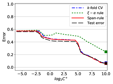
(a) Over $C^{+}$

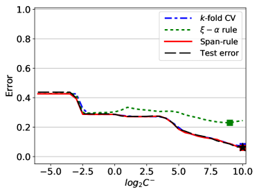
(b) Over $C^{-}$

Figure 2: Image data set. Test error prediction curves and test error curve over each training parameter (Experiment #3). The minimum for each prediction method is marked with a colored “$\square$”; the minimum found test error is marked with a “$\star$”.

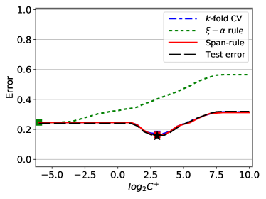
(a) Over $C^{+}$

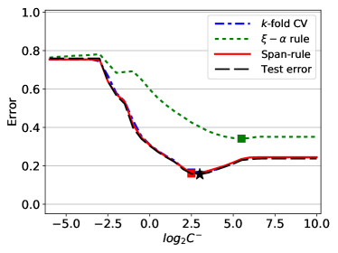
(b) Over $C^{-}$

Figure 3: Adult data set. Test error prediction curves and test error curve over each training parameter (Experiment #3). The minimum for each prediction method is marked with a colored “$\square$”; the minimum found test error is marked with a “$\star$”.

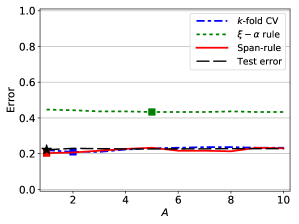
(a) Over $A$

(b) Over $B$

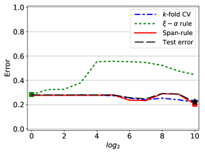
(c) Over $C$

Figure 4: Bank marketing data set. Test error prediction curves and test error curve over each training parameter (Experiment #3). The minimum for each prediction method is marked with a colored “$\square$”; the minimum found test error is marked with a “$\star$”.

Figures 2, 3, and 4 show the test error prediction curves and the test error curve for the image, adult, and bank marketing data sets respectively. In our experiments the weighted SVM models depend on the grid combinations of two training parameters, $(C^{+},C^{-})$, in Experiment #1 and three training parameters, $(A,B,C)$, in Experiment #2. In each sub-plot the curves are plotted against one of the training parameters whereas the values of the other(s) are set to the one(s) that gave the model with the minimum actual test error.

The graphs illustrate that the span-rule for weighted SVM is able to accurately predict the value of the test error over varying parameterizations. Most importantly, span-rule selects parameters that belong in the area around the parameters that yield the minimum test error. Regarding the other hyperparameter selection methods, the $K$-fold cross-validation also performs well. On the other hand, the ${\xi\text{-}\alpha}$ bound is very conservative and fails to predict the value, or even the trend, of the actual test error curve.

6.5 Experiment #4: Is the value of span, $S_{p}$, defined most of the time?

Previous experiments demonstrated that the span-rule for weighted SVM is an effective method for hyperparameter selection and test error prediction. Span-rule is a corollary of Theorem 2 that guarantees ${\Lambda_{p}}\neq\emptyset$ and, thus, the value of $S_{p}$ can always be calculated under theorem’s assumptions.

Nevertheless, it is important to investigate how often the set ${\Lambda_{p}}$ is indeed non-empty by examining how often the inequality of Lemma 1 is satisfied. Table 5 shows the average number of ${\Lambda_{p}}=\emptyset$ occurrences and, for reference, the average number of support vectors per weighted SVM model. The displayed values are averaged over the $1089$ weighted SVM models trained for each data set in Experiment #1 and the $1700$ weighted SVM models trained for each data set in Experiment #2.

Overall, the experiments demonstrate that the occurrence of empty ${\Lambda_{p}}$ is a very rare one. Notably, there is less than one ${\Lambda_{p}}=\emptyset$ occurrence on average for each weighted SVM model and this behavior is consistent across data sets.

Data set	${\Lambda_{p}}=\emptyset$ occurrences	In-bound SVs ($n^{*}$)	Total SVs ($n$)
breast cancer	$0.128$ p m 0.461	$4.6$ p m 2.0	$33.3$ p m 22.6
mushrooms	$0.0$ p m 0.0	$27.6$ p m 10.1	$93.0$ p m 35.9
waveform	$0.003$ p m 0.068	$16.0$ p m 7.2	$188.7$ p m 58.3
banana	$0.0$ p m 0.0	$17.2$ p m 14.	$277.3$ p m 47.1
skin nonskin	$0.197$ p m 0.621	$7.3$ p m 3.8	$167.9$ p m 115.3
splice	$0.0$ p m 0.0	$148.2$ p m 122.9	$581.3$ p m 78.0
image	$0.004$ p m 0.074	$18.8$ p m 7.0	$640.9$ p m 160.2
adult	$0.0$ p m 0.0	$125.8$ p m 83.	$825.9$ p m 289.3
MNIST 2’s vs. 9’s	$0.0$ p m 0.0	$134.6$ p m 108.1	$2368.5$ p m 1828.8
MNIST 1’s vs. 7’s	$0.0$ p m 0.0	$68.6$ p m 44.4	$2210.4$ p m 2056.2
MNIST 3’s vs. 6’s	$0.0$ p m 0.0	$105.8$ p m 69.0	$1935.2$ p m 1711.7
MNIST 0’s vs. 8’s	$0.0$ p m 0.0	$115.5$ p m 88.4	$2028.6$ p m 1721.1
Parkinson’s speech	$0.041$ p m 0.428	$16.1$ p m 10.4	$416.4$ p m 45.8
bank marketing	$0.222$ p m 0.615	$12.5$ p m 9.4	$250.9$ p m 51.2

Table 5: Results for Experiment #4. Average number of ${\Lambda_{p}}=\emptyset$ occurrences and average number of support vectors per data set. The values are calculated using the weighted SVM models trained for each data set in Experiments #1 (1089 models per data set) and Experiment #2 (1700 models per data set).

This finding essentially confirms the assumption of Theorem 2 which asserts that ${\Lambda_{p}}\neq\emptyset$ for all support vectors. Thus, in practice, we can always safely use the span-rule estimator of Corollary 1 by calculating the values of $S_{p}$ for all support vectors of a weighted SVM model.

In addition, the results also affect our understanding for the span bound given by Theorem 1; that is, the span bound for weighted SVM can be as tight as the span bound for standard SVM since the value of $k$, which represents the number of occurrences ${\Lambda_{p}}=\emptyset$, barely affects it.

6.6 Experiment #5: Efficiency evaluation of span-rule and $K$-fold CV

This experiment compares the efficiency between the two most prominent hyperparameter selection methods for weighted SVM: the span-rule and the $K$-fold CV.

Data set	Span-rule	$K$-fold CV
breast cancer	0.031	0.011
mushrooms	0.104	0.056
waveform	0.139	0.090
banana	0.213	0.096
skin nonskin	0.108	0.088
splice	7.637	1.136
image	0.416	0.436
adult	5.567	0.990
MNIST 2’s vs. 9’s	10.423	123.380
MNIST 1’s vs. 7’s	3.069	106.304
MNIST 3’s vs. 6’s	5.116	108.798
MNIST 0’s vs. 8’s	6.410	130.957
Parkinson’s speech	0.278	0.167
bank marketing	0.165	0.060

Table 6: Results for Experiment #5. Average execution time in seconds for span-rule and $K$-fold CV executions of Experiments #1 (1089 executions per data set) and Experiment #2 (1700 executions per data set). Best average execution time is marked with bold font.

Table 6 displays the average execution time needed to calculate the $K$-fold CV and the values of $S_{p}$ for span-rule. The models trained for the $14$ data sets of Experiments #1 and #2 are used. To make the results comparable, we restricted both LibSVM solver and the MOSEK optimizer to one processor. The experiments were executed on a Intel Xeon E5-2650 v3 at 2.3GHz.

Span-rule demonstrates a fairly competitive execution time compared to $K$-fold CV. In most data sets, the span-rule is slightly slower than $K$-fold CV. Usually, such small overheads in training procedure are not very important since, in general, the model training is performed offline and does not affect the use of the trained model in other way.

Notably, the span-rule can be significantly faster than $K$-fold CV on high-dimensional problems with large training sets, such as the four MNIST data sets. To this end, the next and final experiment investigates when is it most efficient to apply the span-rule for weighted SVM hyperparameter selection.

6.7 Experiment #6: When is it faster to use span-rule than $K$-fold CV?

We will investigate how training set size and feature vector dimesionality affect the efficiency of span-rule and $K$-fold CV using synthetic data sets.

Before we delve into the details of the experiment, it is important to understand the differences in executing the span-rule and $K$-fold CV:

• The $K$-fold CV requires the execution $K$ train-test procedures to assess the generalization performance of a given set of parameters. The bulk of the execution time is consumed in solving $K$ quadratic problems with inequality and equality constrains (eq. 5, 6 and 7). Each of the $K$ quadratic problem has $\frac{(K-1)l}{K}$ number of unknown variables, where $l$ is the training set size. Due to the size of these quadratic problems, these are efficiently solved using the Sequential Minimal Optimization (SMO) algorithm (Platt et al., 1999). Furthermore, SVM solvers, such as LibSVM, use a cache to store the most recently calculated kernel products.

• The span-rule requires to solve $n$ quadratic problems for the calculation of $S_{p}$ with $n^{*}$ or $n^{*}+1$ unknown variables for in-bound and bounded support vectors respectively; where $n$ is the total number of support vectors and $n^{*}$ is the number of in-bound support vectors (eq. 28 - 32). In general, for real-word non-separable data sets, the number of supports vectors, $n$, is smaller than the training set size, $l$, and the number of in-bound support vectors, $n^{*}$, is a relatively small percentage of the total number of SVs (see also Table 5). Thus, these quadratic problems can be solved efficiently using general purpose Quadratic Programming solvers, such as the MOSEK optimizer.

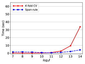
(a) $d=20$

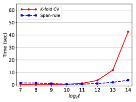
(b) $d=40$

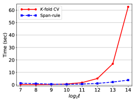
(c) $d=80$

Figure 5: Average execution time of span-rule and $K$-fold CV over varying training set sizes $l$ for feature dimensions $d=20,40,80$ (Experiment #6).

(a) $d=20$

(b) $d=40$

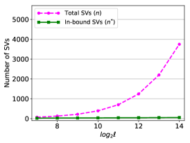
(c) $d=80$

Figure 6: Average number of in-bound and total SVs over varying training set sizes $l$ for feature dimensions $d=20,40,80$ (Experiment #6).

For the synthetic data sets of this experiment, we will use variations of the ringnorm data set of Breiman (1996). The training data are sampled from $d$-dimensional normal distributions, $N({\mathbf{x}};\mu^{+},\Sigma^{+})$ and $N({\mathbf{x}};\mu^{-},\Sigma^{-})$ for the positive and the negative class respectively with priors $Pr\{y=+1\}=0.3$ and $Pr\{y=-1\}=0.7$. For the positive class, we use $\mu^{+}=(1,1,\dots,1)$ and unit covariance matrix $\Sigma^{+}$; for the negative class, we use mean $\mu^{-}=(0,0,\dots,0)$ and $\Sigma^{-}$ equal four times the unit covariance matrix.

For given feature dimension $d$, we create training sets of varying size $l$. We increase the size of the training sets exponentially from $l=2^{7}$ to $l=2^{14}$ and for each training set we execute a full grid search for the optimal values of $C^{+}$ and $C^{-}$ as in Experiment #1.

Figure 5 shows the change in the execution time as the training size, $l$, grows exponentially for the span-rule and $K$-fold CV, using feature dimension, $d$, equal to 20, 40 and 80. Each point on the diagrams represents the average execution time of the corresponding hyperparameter selection method for $1089$ models trained on a full parameter grid search. Similarly, Figure 6 shows the average number of in-bound support vectors and the average number of total (in-bound and bounded) support vectors for the corresponding points.

The experimental results can be interpreted from the following:

• For small training sizes $l$, the $K$-fold CV is marginally faster than span-rule. Also, note that for small $l$ the execution time of $K$-fold CV is practically unaffected by the dimension of the feature space, $d$, due to the fact that most kernel products can be stored in solver’s cache.

• Given feature dimensionality $d$, the span-rule is significantly more efficient than $K$-fold CV for larger training set sizes (for this data set, $l>2^{12}$). As training set size increases, solving the $K$ weighted SVM models becomes computationally harder since it depends directly on $l$. On the other hand, the size of the quadratic problems solved by the span-rule remains small since it depends only on $n^{*}$. Thus, for large training sets, solving $n$ small quadratic problems becomes computationally more attractive than solving $K$ large quadratic problems.

• For large training sizes $l$, the execution time of $K$-fold CV becomes quickly inefficient as the dimensionality $d$ increases. This is due to the fact that computationally expensive kernel products that do not fit in the cache need to be re-calculated. On the other hand, the inner products required for computing the value of the span, $S_{p}$, are calculated only once due to the significantly smaller size of the quadratic problems.

In conclusion, the results of Experiments #5 and #6 demonstrate that the efficiency of span-rule compared to $K$-fold CV increases as: (a) the dimensionality of the feature space increases; and (b) the size of the training set increases, given that the number of in-bound support vectors, $n^{*}$, remains relatively small.

6.8 Summary of experimental findings

In this section, we experimentally evaluated four hyperparameter selection methods applicable to weighted SVM: the span-rule of Corollary 1, the span bound of Theorem 1, the $K$-fold CV (with $K=5$) and the ${\xi\text{-}\alpha}$ bound. We evaluated the effectiveness and the efficiency of the hyperparameter selection methods on $14$ data sets in two experimental settings. Furthermore, we examined how often the existence condition of Lemma 1 holds, which is the basis for the span error bound theory for weighted SVM.

The key experimental findings are:

• The span-rule is the most effective method for weighted SVM hyperparameter selection (Experiments #1 and #2).

• The span-rule is the best predictor for the value of the actual test error in the mean-square-error sense (Experiment #3).

• The condition of Lemma 1 that ensures that ${\Lambda_{p}}\neq\emptyset$ is satisfied almost always (Experiment #4). This experimental observation verifies the theoretical assumptions used to derive the span-rule for weighted SVM and ensures that we can safely apply it in practical problems.

• The span-rule is a fairly efficient method for hyperparameter selection especially for problems with large training sets and high-dimensional feature spaces (Experiments #5 and #6).

7 Conclusions

In this work, we presented the extension of the span error bound theory of Vapnik and Chapelle (2000) to weighted SVM. The ground for this extension is the proof for the necessary and sufficient condition for defining the span of a support vector in a weighted SVM model (Lemma 1). Building on this, we prove the span bound (Theorem 1) and the span-rule (Corollary 1) for weighted SVM algorithm. Furthermore, we prove that, under the assumption that the support vectors do not change, the span is defined for all support vectors of a weighted SVM solution (Theorem 2).

The extended theory enables new and effective tools for weighted SVM hyperparameter selection. We experimentally evaluate the presented span bound for weighted SVM, the presented span-rule for weighted SVM, the $K$-fold cross-validation (with $K=5$) and the ${\xi\text{-}\alpha}$ bound on $14$ standard benchmark data sets and data sets with instance importance scores.

The experiments demonstrate the practical value of the span error bound theory for weighted SVM. Using the span-rule we are able to efficienlty select training parameters that lead to small testing error. Furthermore, using the span-rule we can accurately predict the value of the actual test error in the mean-square-error sense. Compared to the other methods, the span-rule demonstrates a considerable improvement over the $K$-fold cross-validation and performs significantly better than the ${\xi\text{-}\alpha}$ bound.

Additional experiments analyzing several thousands of weighted SVM models trained on all data sets confirmed that the condition of Lemma 1 holds true virtually for all support vectors. This finding ensures that we can safely apply the span-rule for weighted SVM in practical problems.

Apart from the practical applications of the span-rule for hyperparameter selection tasks, the presented work allows further theoretical investigation for the weighted SVM algorithm. Most importantly, new theoretical tools are enabled—based on the geometrical concept of the span—for understanding the effect of the instance weights and their role in the generalization performance of the weighted SVM algorithm.

Appendix A. Proofs

A.1   Proof of Lemma 1

In the first part of the proof, we show the sufficient condition for the existence of ${\Lambda_{p}}$ for an in-bound support vector ${\mathbf{x}}_{p}$ of a weighted SVM solution. In the second part, we prove that the condition is also necessary.

Sufficiency: Based on the proof of Vapnik and Chapelle (2000) for standard SVM in the non-separable case, let the set

$${\Lambda_{p}}^{+}=\left\{{\mathbf{x}}~{}:~{}{\mathbf{x}}={\sum\limits_{i=1,i\neq p}^{n^{*}}}{\lambda}_{i}{\mathbf{x}}_{i}\in{\Lambda_{p}},\text{ and }{\lambda}_{i}\geq 0~{}~{}\forall i\neq p\right\}$$ (40)

Because ${\Lambda_{p}}^{+}\subseteq{\Lambda_{p}}$, proving that ${\Lambda_{p}}^{+}\neq\emptyset$ under the Lemma’s condition also implies that the same condition suffices for ${\Lambda_{p}}\neq\emptyset$.

In view of (24), ${\Lambda_{p}}^{+}$ contains exactly the linear combinations ${\sum\limits_{i=1,i\neq p}^{n^{*}}}{\lambda}_{i}{\mathbf{x}}_{i}$ that satisfy:

$${\sum\limits_{i=1,i\neq p}^{n^{*}}}{\lambda}_{i}=1$$ (41)

$$0\leq{\alpha}^{0}_{i}+y_{i}y_{p}{\alpha}^{0}_{p}{\lambda}_{i}\leq C_{i},~{}~{}~{}\forall i\neq p,~{}~{}i=1,\dots,n^{*}$$ (42)

$${\lambda}_{i}\geq 0,~{}~{}~{}\forall i\neq p,~{}~{}i=1,\dots,n^{*}$$ (43)

Equations (42) and (43) can be expressed through the alternative conditions:

$${\lambda}_{i}=\mu\frac{C_{i}-{\alpha}_{i}^{0}}{{\alpha}_{p}^{0}},~{}~{}y_{i}=y_{p},~{}~{}i\neq p,~{}~{}i=1,\dots,n^{*}$$ (44)

$${\lambda}_{i}=\mu\frac{{\alpha}_{i}^{0}}{{\alpha}_{p}^{0}},~{}~{}y_{i}\neq y_{p},~{}~{}i=1,\dots,n^{*}$$ (45)

$$0\leq\mu\leq 1$$ (46)

Our target is now to show that condition of Lemma 1 (eq. 25) guarantees that an appropriate $\mu$ exists that makes (41), (44), (45), (46) hold simultaneously true.

Substituting equations (44) and (45) into (41) gives

$$1=\frac{\mu}{{\alpha}_{p}^{0}}\left({\sum\limits_{\begin{subarray}{c}i=1,i\neq p,\\ y_{i}=y_{p}\end{subarray}}^{n^{*}}}(C_{i}-{\alpha}_{i}^{0})+{\sum\limits_{\begin{subarray}{c}i=1,\\ y_{i}\neq y_{p}\end{subarray}}^{n^{*}}}{\alpha}_{i}^{0}\right)$$ (47)

Let ${\Delta}$ be the positive quantity:

$${\Delta} ={\sum\limits_{\begin{subarray}{c}i=1,\\ y_{i}=y_{p}\end{subarray}}^{n^{*}}}(C_{i}-{\alpha}_{i}^{0})+{\sum\limits_{\begin{subarray}{c}i=1,\\ y_{i}\neq y_{p}\end{subarray}}^{n^{*}}}{\alpha}_{i}^{0}$$

$$=-y_{p}{\sum\limits_{i=1}^{n^{*}}}y_{i}{\alpha}_{i}^{0}+{\sum\limits_{\begin{subarray}{c}i=1,\\ y_{i}=y_{p}\end{subarray}}^{n^{*}}}C_{i}$$ (48)

Using ${\Delta}$ we can write equation (47) as

$$1=\frac{\mu}{{\alpha}_{p}^{0}}({\Delta}-(C_{p}-{\alpha}_{p}^{0}))$$ (49)

Hence, equation (41) is satisfied for

$$\mu=\frac{a_{p}^{0}}{{\Delta}-C_{p}+a_{p}^{0}}$$ (50)

It remains to show that this value of $\mu$ also satisfies equation (46). Indeed, if the condition (25) of Lemma 1 holds true for an in-bound support vector ($p=1,\dots,n^{*}$), then

$${\sum\limits_{\begin{subarray}{c}i=1,i\neq p,\\ y_{i}=y_{p}\end{subarray}}^{n^{*}}}C_{i}\geq-y_{p}{\sum\limits_{i=n^{*}+1}^{n}}y_{i}C_{i}$$

and the following holds true

$${\Delta}-C_{p} =-y_{p}{\sum\limits_{i=1}^{n^{*}}}y_{i}{\alpha}_{i}^{0}+{\sum\limits_{\begin{subarray}{c}i=1,i\neq p,\\ y_{i}=y_{p}\end{subarray}}^{n^{*}}}C_{i}$$

$$\geq-y_{p}{\sum\limits_{i=1}^{n^{*}}}y_{i}{\alpha}_{i}^{0}-y_{p}{\sum\limits_{i=n^{*}+1}^{n}}y_{i}C_{i}$$

$$=-y_{p}\left({\sum\limits_{i=1}^{n^{*}}}y_{i}{\alpha}_{i}^{0}+{\sum\limits_{i=n^{*}+1}^{n}}y_{i}C_{i}\right)$$ (51)

From the constraint (7) of weighted SVM dual problem, it is

$${\sum\limits_{i=1}^{n}}y_{i}{\alpha}_{i}^{0}={\sum\limits_{i=1}^{n^{*}}}y_{i}{\alpha}_{i}^{0}+{\sum\limits_{i=n^{*}+1}^{n}}y_{i}C_{i}=0$$ (52)

Substituting (52) into (51) yields

$${\Delta}-C_{p}\geq 0$$ (53)

Thus, from (50) and (53) we can show that the condition (46) is satisfied as well.

Necessity: We will show that (25) is also a necessary condition. The box constraints of ${\Lambda_{p}}$ (eq. 24) can be written as

$$0\leq{\alpha}_{i}^{0}+{\alpha}_{p}^{0}{\lambda}_{i}\leq C_{i},~{}~{} y_{i}=y_{p},~{}~{}i=1,\dots,n^{*},~{}~{}i\neq p$$ (54)

$$0\leq{\alpha}_{i}^{0}-{\alpha}_{p}^{0}{\lambda}_{i}\leq C_{i},~{}~{} y_{i}\neq y_{p},~{}~{}i=1,\dots,n^{*}$$ (55)

From the summation of the inequalities given by (54) we get

$$0\leq{\sum\limits_{\begin{subarray}{c}i=1,i\neq p,\\ y_{i}=y_{p}\end{subarray}}^{n^{*}}}{\alpha}_{i}^{0}+{\alpha}_{p}^{0}{\sum\limits_{\begin{subarray}{c}i=1,i\neq p,\\ y_{i}=y_{p}\end{subarray}}^{n^{*}}}{\lambda}_{i}\leq{\sum\limits_{\begin{subarray}{c}i=1,i\neq p,\\ y_{i}=y_{p}\end{subarray}}^{n^{*}}}C_{i}$$ (56)

Similarly, from the inequalities given by (55) we get

$$0\leq{\sum\limits_{\begin{subarray}{c}i=1,\\ y_{i}\neq y_{p}\end{subarray}}^{n^{*}}}{\alpha}_{i}^{0}-{\alpha}_{p}^{0}{\sum\limits_{\begin{subarray}{c}i=1,\\ y_{i}\neq y_{p}\end{subarray}}^{n^{*}}}{\lambda}_{i}\leq{\sum\limits_{\begin{subarray}{c}i=1,\\ y_{i}\neq y_{p}\end{subarray}}^{n^{*}}}C_{i}$$ (57)

By rewriting (57) as

$$-{\sum\limits_{\begin{subarray}{c}i=1,\\ y_{i}\neq y_{p}\end{subarray}}^{n^{*}}}C_{i}\leq-{\sum\limits_{\begin{subarray}{c}i=1,\\ y_{i}\neq y_{p}\end{subarray}}^{n^{*}}}{\alpha}_{i}^{0}+{\alpha}_{p}^{0}{\sum\limits_{\begin{subarray}{c}i=1,\\ y_{i}\neq y_{p}\end{subarray}}^{n^{*}}}{\lambda}_{i}\leq 0$$ (58)

and taking the summation of (56) and (58) we have

$$-{\sum\limits_{\begin{subarray}{c}i=1,\\ y_{i}\neq y_{p}\end{subarray}}^{n^{*}}}C_{i}\leq{\sum\limits_{\begin{subarray}{c}i=1,i\neq p,\\ y_{i}=y_{p}\end{subarray}}^{n^{*}}}{\alpha}_{i}^{0}+{\alpha}_{p}^{0}{\sum\limits_{\begin{subarray}{c}i=1,i\neq p,\\ y_{i}=y_{p}\end{subarray}}^{n^{*}}}{\lambda}_{i}-{\sum\limits_{\begin{subarray}{c}i=1,\\ y_{i}\neq y_{p}\end{subarray}}^{n^{*}}}{\alpha}_{i}^{0}+{\alpha}_{p}^{0}{\sum\limits_{\begin{subarray}{c}i=1,\\ y_{i}\neq y_{p}\end{subarray}}^{n^{*}}}{\lambda}_{i}\leq{\sum\limits_{\begin{subarray}{c}i=1,i\neq p,\\ y_{i}=y_{p}\end{subarray}}^{n^{*}}}C_{i}~{}\Leftrightarrow$$

$$-{\sum\limits_{\begin{subarray}{c}i=1,\\ y_{i}\neq y_{p}\end{subarray}}^{n^{*}}}C_{i}\leq y_{p}{\sum\limits_{i=1,i\neq p}^{n^{*}}}y_{i}{\alpha}_{i}^{0}+{\alpha}_{p}^{0}{\sum\limits_{i=1,i\neq p}^{n^{*}}}{\lambda}_{i}\leq{\sum\limits_{\begin{subarray}{c}i=1,i\neq p,\\ y_{i}=y_{p}\end{subarray}}^{n^{*}}}C_{i}~{}\Leftrightarrow$$

$$-{\sum\limits_{\begin{subarray}{c}i=1,\\ y_{i}\neq y_{p}\end{subarray}}^{n^{*}}}C_{i}-y_{p}{\sum\limits_{i=1}^{n^{*}}}y_{i}{\alpha}_{i}^{0}\leq{\alpha}_{p}^{0}\left({\sum\limits_{i=1,i\neq p}^{n^{*}}}{\lambda}_{i}-1\right)\leq{\sum\limits_{\begin{subarray}{c}i=1,i\neq p,\\ y_{i}=y_{p}\end{subarray}}^{n^{*}}}C_{i}-y_{p}{\sum\limits_{i=1}^{n^{*}}}y_{i}{\alpha}_{i}^{0}$$ (59)

By definition (eq. 24) the existence of the set ${\Lambda_{p}}$ requires

$${\sum\limits_{i=1,i\neq p}^{n^{*}}}{\lambda}_{i}=1$$ (60)

Substituting (60) into (59) gives the following two necessary conditions for ${\Lambda_{p}}\neq\emptyset$

$$-{\sum\limits_{\begin{subarray}{c}i=1,\\ y_{i}\neq y_{p}\end{subarray}}^{n^{*}}}C_{i}-y_{p}{\sum\limits_{i=1}^{n^{*}}}y_{i}{\alpha}_{i}^{0}\leq 0$$ (61)

$${\sum\limits_{\begin{subarray}{c}i=1,i\neq p,\\ y_{i}=y_{p}\end{subarray}}^{n^{*}}}C_{i}-y_{p}{\sum\limits_{i=1}^{n^{*}}}y_{i}{\alpha}_{i}^{0}\geq 0$$ (62)

We can write (61) as

$$-{\sum\limits_{\begin{subarray}{c}i=1,\\ y_{i}\neq y_{p}\end{subarray}}^{n^{*}}}(C_{i}-{\alpha}_{i})-{\sum\limits_{\begin{subarray}{c}i=1,\\ y_{i}=y_{p}\end{subarray}}^{n^{*}}}{\alpha}_{i}\leq 0$$

which is always satisfied since $0<{\alpha}_{i}<C_{i}$ for $i=1,\dots,n^{*}$.

The inequality (62) can be written using (52) as

$${\sum\limits_{\begin{subarray}{c}i=1,i\neq p,\\ y_{i}=y_{p}\end{subarray}}^{n^{*}}}C_{i}+y_{p}{\sum\limits_{i=n^{*}+1}^{n}}y_{i}C_{i}\geq 0$$ (63)

We observe that the necessary condition (63) coincides with the lemma’s condition (eq. 25) and the lemma is proved.

Remark: Similar to standard SVM, when ${\Lambda_{p}}^{+}$ exists, and because it is a convex combination of the in-bound support vectors (eq. 40), it holds that: $d({\mathbf{x}}_{p},{\Lambda_{p}}^{+})\leq D_{SV}$, where $D_{SV}$ is the diameter of the sphere enclosing the in-bound support vectors. Also, since ${\Lambda_{p}}^{+}\subseteq{\Lambda_{p}}$ we get

$$S_{p}=d({\mathbf{x}}_{p},{\Lambda_{p}})\leq d({\mathbf{x}}_{p},{\Lambda_{p}}^{+})\leq D_{SV}$$

A.2   Proof of Theorem 1

The instances that are not support vectors are correctly classified by the initial model. Also, their removal from the training set does not change the decision function. Therefore, these training instances do not contribute in the number of leave-one-out errors.

Considering the $k$ in-bound support vectors that do not satisfy the condition of Lemma 1 and the $m$ bounded support vectors as leave-one-out errors, then

$$\mathcal{L}({\mathbf{x}}_{1},y_{1}\dots,{\mathbf{x}}_{l},y_{l}) \leq\mathcal{L}^{*}({\mathbf{x}}_{1},y_{1},\dots,{\mathbf{x}}_{l},y_{l})+k+m$$ (64)

where $\mathcal{L}^{*}({\mathbf{x}}_{1},y_{1},\dots,{\mathbf{x}}_{l},y_{l})$ is the number of leave-one-out errors originating by the $n^{*}-k$ in-bound support vectors with ${\Lambda_{p}}\neq\emptyset$.

In view of Lemma 2 the following inequality holds true

$$\mathcal{L}^{*}({\mathbf{x}}_{1},y_{1},\dots,{\mathbf{x}}_{l},y_{l})\leq\sum_{p=1}^{n^{*}-k}{\alpha}_{p}^{0}S_{p}max(D,1/\sqrt{C_{p}})$$ (65)

Substituting (65) into (64) we have:

$$\mathcal{L}({\mathbf{x}}_{1},y_{1}\dots,{\mathbf{x}}_{l},y_{l}) \leq\sum_{p=1}^{n^{*}-k}[S_{p}\max(D,1/\sqrt{C_{p}}){\alpha}_{p}^{0}]+k+m$$ (66)

$$\leq S\sum_{p=1}^{n^{*}-k}[\max(D,1/\sqrt{C_{p}}){\alpha}_{p}^{0}]+k+m$$ (67)

where we used the value of $S$-span from (33).

Dividing both sides of (67) by $l$ and taking the expectation over the ensemble of training sets of size $l$, we get

$$E_{{T}_{l}}\left[{R_{\text{\tiny LOO}}}({T}_{l})\right]\leq E_{{T}_{l}}\left[\frac{S\sum_{p=1}^{n^{*}-k}[\max(D,1/\sqrt{C_{p}}){\alpha}_{p}^{0}]+k+m}{l}\right]$$ (68)

Finally, the theorem is proved by applying the leave-one-out theorem (eq. 19) for the left-hand side of inequality (68).

A.3   Proof of Theorem 2

Let ${\bm{\alpha}}^{0}=({\alpha}_{1}^{0},\dots,{\alpha}_{n}^{0},0,\dots,0)$ be the initial solution on the complete training set that maximizes the objective functional $W({\bm{\alpha}})$ of the dual problem of weighted SVM (eq. 5).

Let ${\mathbf{x}}_{p}$ be a fixed support vector (either in-bound or bounded) for which a leave-one-out model is trained. Under the assumption that the in-bound and bounded sets of support vectors do not change, let the vector of Lagrange multipliers of the optimal solution on the reduced training set:

$${\bm{\alpha}}^{p}=({\alpha}_{1}^{p},\dots,{\alpha}_{p-1}^{p},0,{\alpha}_{p+1}^{p},{\alpha}_{n}^{0},0,\dots,0)$$

Proof of ${\Lambda_{p}}\neq\emptyset$: We will show that ${\Lambda_{p}}\neq\emptyset$ by finding a fixed vector ${\bm{\lambda}}^{\prime}$ that satisfies both the linear constraint and the box constraints of (24).

Using ${\bm{\alpha}}^{0}$ and ${\bm{\alpha}}^{p}$ we set the elements of ${\bm{\lambda}}^{\prime}$ as:

$${\lambda}_{i}^{\prime}=y_{i}y_{p}\frac{{\alpha}_{i}^{p}-{\alpha}_{i}^{0}}{{\alpha}_{p}^{0}},~{}~{}~{}i=1\dots,n^{*},~{}i\neq p$$ (69)

The box constrains of (24) are satisfied for ${\bm{\lambda}}^{\prime}$ since

$$0\leq{\alpha}^{0}_{i}+y_{i}y_{p}{\alpha}^{0}_{p}{\lambda}_{i}^{\prime}\leq C_{i}~{}\Leftrightarrow$$

$$0\leq{\alpha}_{i}^{0}+y_{i}y_{p}{\alpha}^{0}_{p}y_{i}y_{p}\frac{{\alpha}_{i}^{p}-{\alpha}_{i}^{0}}{{\alpha}_{p}^{0}}\leq C_{i}~{}\Leftrightarrow$$

$$0\leq{\alpha}_{i}^{p}\leq C_{i}$$

which holds true.

For ${\bm{\lambda}}^{\prime}$, the left-hand side of the linear constraint of (24) can be written using (69) as

$${\sum\limits_{i=1,i\neq p}^{n^{*}}}{\lambda}_{i}^{\prime}=\frac{y_{p}}{{\alpha}_{p}^{0}}\left({\sum\limits_{i=1,i\neq p}^{n^{*}}}y_{i}{\alpha}_{i}^{p}-{\sum\limits_{i=1,i\neq p}^{n^{*}}}y_{i}{\alpha}_{i}^{0}\right)$$ (70)

From the constraint (7) of dual problem, and considering that ${\mathbf{x}}_{p}$ can be either in-bound or bounded ($0<{\alpha}_{p}^{0}\leq C_{p}$), the following holds for the initial solution ${\bm{\alpha}}^{0}$

$${\sum\limits_{i=1}^{n}}y_{i}{\alpha}_{i}^{0}={\sum\limits_{i=1}^{n^{*}}}y_{i}{\alpha}_{i}^{0}+{\sum\limits_{i=n^{*}+1}^{n}}y_{i}C_{i}=0~{}\Leftrightarrow$$

$${\sum\limits_{i=1,i\neq p}^{n^{*}}}y_{i}{\alpha}_{i}^{0}+{\sum\limits_{i=n^{*}+1,i\neq p}^{n}}y_{i}C_{i}+y_{p}{\alpha}_{p}^{0}=0$$ (71)

Similarly, from (7) for the leave-one-out solution ${\bm{\alpha}}^{p}$ (where ${\alpha}_{p}^{p}=0$) it is

$${\sum\limits_{i=1,i\neq p}^{n^{*}}}y_{i}{\alpha}_{i}^{p}+{\sum\limits_{i=n^{*}+1,i\neq p}^{n}}y_{i}C_{i}=0$$ (72)

Using (71) and (72) we can write (70) as

$${\sum\limits_{i=1,i\neq p}^{n^{*}}}{\lambda}_{i}^{\prime}=\frac{y_{p}}{{\alpha}_{p}^{0}}\left(-{\sum\limits_{i=n^{*}+1,i\neq p}^{n}}y_{i}C_{i}+{\sum\limits_{i=n^{*}+1,i\neq p}^{n}}y_{i}C_{i}+y_{p}{\alpha}_{p}^{0}\right)=\frac{y_{p}}{{\alpha}_{p}^{0}}\cdot y_{p}{\alpha}_{p}^{0}=1$$

Hence, the linear combination ${\bm{\lambda}}^{\prime}={\sum\limits_{i=1,i\neq p}^{n^{*}}}{\lambda}_{i}^{\prime}{\mathbf{x}}_{i}$ belongs in ${\Lambda_{p}}$. Thus, the set ${\Lambda_{p}}$ is non-empty for any support vector ${\mathbf{x}}_{p}$ under theorem’s assumption.

Proof of theorem’s equality: This part of the proof is omitted due to its similarity to the proof of Theorem 2.3 of Vapnik and Chapelle (2000).

References

- Barrett et al. (2009) S. Barrett, R. Chang, and X. Qi. A fuzzy combined learning approach to content-based image retrieval. In 2009 IEEE International Conference on Multimedia and Expo, pages 838–841, June 2009.
- Bicego and Figueiredo (2009) Manuele Bicego and Mario A.T. Figueiredo. Soft clustering using weighted one-class support vector machines. Pattern Recognition, 42(1):27 – 32, 2009. ISSN 0031-3203.
- Breiman (1996) L. Breiman. Bias, variance, and arcing classifiers, 1996. Available Online.
- Chang and Lin (2011) C.-C. Chang and C.-J. Lin. LIBSVM: A library for support vector machines. ACM Transactions on Intelligent Systems and Technology, 2(3):27:1–27:27, 2011.
- Chapelle and Vapnik (2000) O. Chapelle and V. Vapnik. Model selection for support vector machines. In Advances in Neural Information Processing Systems, pages 230–236. MIT Press, 2000.
- Chapelle et al. (2002) O. Chapelle, V. Vapnik, O. Bousquet, and S. Mukherjee. Choosing multiple parameters for support vector machines. Machine Learning, 46(1-3):131–159, 2002.
- Chaudhuri and De (2011) Arindam Chaudhuri and Kajal De. Fuzzy support vector machine for bankruptcy prediction. Applied Soft Computing, 11(2):2472 – 2486, 2011. ISSN 1568-4946.
- Cheng et al. (2016) Y. W. Cheng, T. J. Wen, H. C. Cheng, and C. Y. Yang. Distance weighted fuzzy k-NN SVM. In 2016 IEEE 13th International Conference on Networking, Sensing, and Control (ICNSC), pages 1–6, April 2016.
- Crisp and Burges (1999) D. Crisp and C. Burges. Uniqueness of the SVM solution. In Proceedings of the 1999 Conference on Advances in Neural Information Processing Systems, volume 12, page 223. MIT Press, 1999.
- (10) Delve. Delve datasets. URL http://www.cs.toronto.edu/~delve/data/datasets.html.
- Duan et al. (2003) K. Duan, S. S. Keerthi, and A. N. Poo. Evaluation of simple performance measures for tuning SVM hyperparameters. Neurocomputing, 51:41–59, 2003.
- Goetz et al. (2008) Christopher G. Goetz, Barbara C. Tilley, Stephanie R. Shaftman, Glenn T. Stebbins, Stanley Fahn, Pablo Martinez-Martin, Werner Poewe, Cristina Sampaio, Matthew B. Stern, Richard Dodel, Bruno Dubois, Robert Holloway, Joseph Jankovic, Jaime Kulisevsky, Anthony E. Lang, Andrew Lees, Sue Leurgans, Peter A. LeWitt, David Nyenhuis, C. Warren Olanow, Olivier Rascol, Anette Schrag, Jeanne A. Teresi, Jacobus J. van Hilten, and Nancy LaPelle. Movement disorder society-sponsored revision of the unified parkinson’s disease rating scale (mds-updrs): Scale presentation and clinimetric testing results. Movement Disorders, 23(15):2129–2170, 2008. ISSN 1531-8257.
- Hsu et al. (2009) C.-C. Hsu, M.-F. Han, S.-H. Chang, and H.-Y. Chung. Fuzzy support vector machines with the uncertainty of parameter C. Expert Systems with Applications, 36(3, Part 2):6654–6658, 2009.
- Huang and Wang (2006) C.-L. Huang and C.-J. Wang. A GA-based feature selection and parameters optimizationfor support vector machines. Expert Systems with Applications, 31(2):231–240, 2006.
- (15) IDA. Ida benchmark repository. URL http://mldata.org/repository/tags/data/IDA\_Benchmark\_Repository/.
- Jaakkola and Haussler (1999) T. S. Jaakkola and D. Haussler. Probabilistic kernel regression models. In Proceedings of the 1999 Conference on AI and Statistics. Morgan Kaufmann, 1999.
- Joachims (2000) T. Joachims. Estimating the generalization performance of an svm efficiently. In Proceedings of the Seventeenth International Conference on Machine Learning, pages 431–438. Morgan Kaufmann Publishers Inc., 2000.
- Keerthi (2002) S. S. Keerthi. Efficient tuning of svm hyperparameters using radius/margin bound and iterative algorithms. IEEE Transactions on Neural Networks, 13(5):1225–1229, Sep 2002.
- Lapin et al. (2014) Maksim Lapin, Matthias Hein, and Bernt Schiele. Learning using privileged information: SVM+ and weighted SVM. Neural Networks, 53:95 – 108, 2014. ISSN 0893-6080.
- Lecun et al. (1998) Y. Lecun, L. Bottou, Y. Bengio, and P. Haffner. Gradient-based learning applied to document recognition. Proceedings of the IEEE, 86(11):2278–2324, Nov 1998. ISSN 0018-9219.
- Lichman (2013) M. Lichman. UCI machine learning repository, 2013. URL http://archive.ics.uci.edu/ml.
- Lin and Wang (2002) C.-F. Lin and S.-D. Wang. Fuzzy support vector machines. IEEE Transactions on Neural Networks, 13(2):464–471, 2002.
- Lin and Wang (2004) C.-F. Lin and S.-D. Wang. Training algorithms for fuzzy support vector machines with noisy data. Pattern Recognition Letters, 25(14):1647 – 1656, 2004.
- Lin et al. (2008) S.-W. Lin, K.-C. Ying, S.-C. Chen, and Z.-J. Lee. Particle swarm optimization for parameter determination and feature selection of support vector machines. Expert Systems with Applications, 35(4):1817–1824, 2008.
- Luntz and Brailovsky (1969) A. Luntz and V. Brailovsky. On estimation of characters obtained in statistical procedure of recognition (in russian). Technicheskaya Kibernetica, 3, 1969.
- Moro et al. (2014) Sérgio Moro, Paulo Cortez, and Paulo Rita. A data-driven approach to predict the success of bank telemarketing. Decision Support Systems, 62:22 – 31, 2014. ISSN 0167-9236.
- MOSEK ApS (2017) MOSEK ApS. MOSEK Optimizer API for Python. Version 8.1., 2017. URL http://docs.mosek.com/8.1/pythonapi/index.html.
- Opper and Winther (2000) M. Opper and O. Winther. Gaussian processes and SVM: mean field and leave-one-out. In A.J. Smola, P.L. Bartlett, B. Schölkopf, and D. Schuurmans, editors, Advances in Large Margin Classifiers, pages 311–326, Cambridge, MA, 2000. MIT Press.
- Papapanagiotou et al. (2015) V. Papapanagiotou, C. Diou, and A. Delopoulos. Improving concept-based image retrieval with training weights computed from tags. ACM Transactions on Multimedia Computing, Communications, and Applications, 12(2):32:1–32:22, 2015.
- Platt et al. (1999) John Platt et al. Fast training of support vector machines using sequential minimal optimization. Advances in kernel methods—-support vector learning, 3:185–208, 1999.
- Sakar et al. (2013) B. E. Sakar, M. E. Isenkul, C. O. Sakar, A. Sertbas, F. Gurgen, S. Delil, H. Apaydin, and O. Kursun. Collection and analysis of a parkinson speech dataset with multiple types of sound recordings. IEEE Journal of Biomedical and Health Informatics, 17(4):828–834, July 2013. ISSN 2168-2194.
- Sarafis et al. (2015) I. Sarafis, C. Diou, and A. Delopoulos. Building effective SVM concept detectors from clickthrough data for large-scale image retrieval. International Journal of Multimedia Information Retrieval, 4(2):129–142, 2015.
- Sarafis et al. (2016) I. Sarafis, C. Diou, and A. Delopoulos. Online training of concept detectors for image retrieval using streaming clickthrough data. Engineering Applications of Artificial Intelligence, 51:150 – 162, 2016.
- Schölkopf and Smola (2002) B. Schölkopf and A. J. Smola. Learning with kernels: support vector machines, regularization, optimization, and beyond. MIT press, 2002.
- Vapnik (1998) V. Vapnik. Statistical learning theory. Wiley New York, 1998.