Saturating the quantum Cramér-Rao bound using LOCC

Abstract

The quantum Cramér-Rao bound (QCRB) provides an ultimate precision limit allowed by quantum mechanics in parameter estimation. Given any quantum state dependent on a single parameter, there is always a positive-operator valued measurement (POVM) saturating the QCRB. However, the QCRB-saturating POVM cannot always be implemented efficiently, especially in multipartite systems. In this paper, we show that the POVM based on local operations and classical communication (LOCC) is QCRB-saturating for arbitrary pure states or rank-two mixed states with varying probability distributions over fixed eigenbasis. Local measurements without classical communication, however, is not QCRB-saturating in general.

I Introduction

Quantum metrology Giovannetti et al. (2006, 2011); Degen et al. (2017); Braun et al. (2018); Pezzè et al. (2018); Pirandola et al. (2018) is the study of designing high-precision quantum sensors to estimate physical parameters in quantum systems. It focuses on the ultimate precision achievable in parameter estimation, allowed by the theory of quantum mechanics. It has wide applications ranging from frequency spectroscopy and clocks Sanders and Milburn (1995); Bollinger et al. (1996); Huelga et al. (1997); Leibfried et al. (2004); Giovannetti et al. (2004); Bu$\mathbf{z}$ek et al. (1999); Valencia et al. (2004); de Burgh and Bartlett (2005) to gravitational-wave detectors and interferometry Caves (1981); Yurke et al. (1986); Berry and Wiseman (2000); Higgins et al. (2007). Lying in the center of quantum metrology is the quantum Cramér-Rao bound (QCRB) Helstrom (1976, 1968); Paris (2009); Braunstein and Caves (1994), which provides a lower bound of parameter estimation error:

$$\delta\theta\geq\frac{1}{\sqrt{NJ(\rho_{\theta})}}.$$ (1)

Here $\theta$ is the parameter to be estimated, e.g. magnetic field frequency, $\delta\theta$ is the standard deviation of the $\theta$-estimator, $\rho_{\theta}$ is the density matrix describing the quantum sensor as a function of $\theta$, and $N$ is the number of repeated experiments. $J(\rho_{\theta})$ is the so-called quantum Fisher information (QFI) Helstrom (1976, 1968); Paris (2009); Braunstein and Caves (1994) quantifying the sensitivity of a quantum sensor.

QFI can be viewed as the maximum Fisher information (FI) among all possible POVMs, where FI is the classical version of QFI as a measure of sensitivity Kobayashi et al. (2011); Casella and Berger (2002); Lehmann and Casella (2006). It is a function of the probability distribution of measurement results. In a quantum system, the probability distribution is provided by $P_{x}(\theta)=\mathrm{Tr}(\rho_{\theta}E_{x})$ with measurement operators $\{E_{x}\}$. To saturate the QCRB, one first performs the optimal POVM maximizing the FI Braunstein and Caves (1994), and then chooses suitable classical estimators, e.g. the maximum likelihood estimator which asymptotically ($N\gg 1$) saturates the QCRB Lehmann and Casella (2006); Casella and Berger (2002); Brody and Hughston (1996); Fujiwara (2006). The optimal POVM usually depends on the value of the parameter, which is unknown practically. In order to solve this issue, one could use the two-step method by first using $\sqrt{N}$ states to obtain a rough estimation $\tilde{\theta}\approx\theta$ and then performing the optimal measurement based on $\tilde{\theta}$ on the remaining $N-\sqrt{N}$ states Barndorff-Nielsen and Gill (2000); Hayashi (2011); Yang et al. (2019a). The procedure introduces a negligible amount of error asymptotically. If the problem was approached using a Bayesian approach, under quite general conditions, the QFI remains a reliable figure of merit Lehmann and Casella (2006); Gill (2008); Pezze and Smerzi (2014); Jarzyna and Demkowicz-Dobrzański (2015); Górecki et al. (2020). It is known that rank-one projection onto the eigenstates of the symmetric logarithmic derivative operator (SLD) usually saturates the QCRB Braunstein and Caves (1994). However, in general, the eigenstates of SLD could be highly-entangled states over subsystems, and the optimal measurement requires global measurements (GM) (Fig. 1a) that might be challenging to implement experimentally Friis et al. (2017).

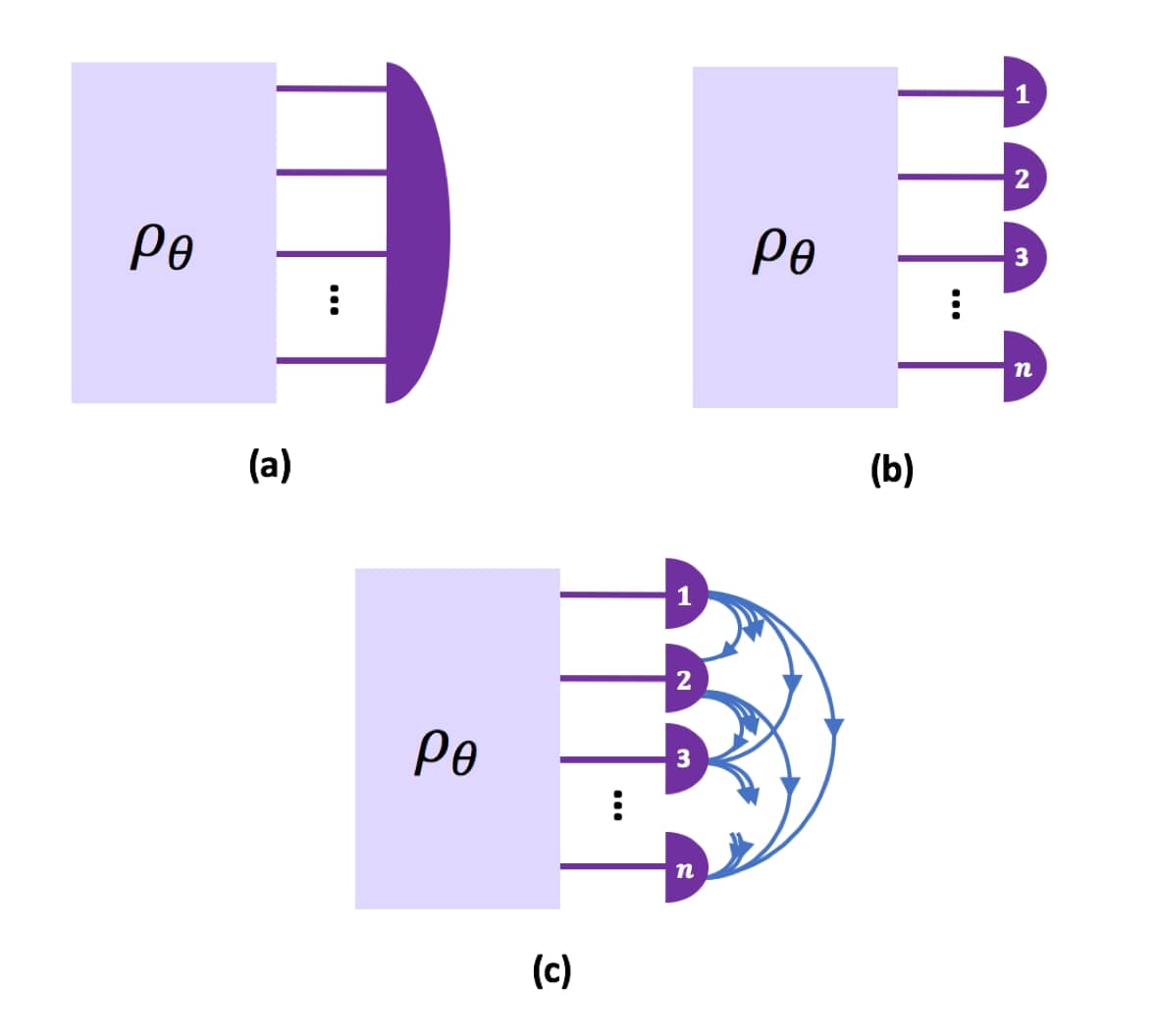
Figure 1: Schematics of measurement protocols in quantum metrology. Here, ${\rm LM}\subseteq{\rm LOCC}\subseteq{\rm GM}$. (a) Global measurements (GM). (b) Local measurements (LM). (c) Local operations and classical communication (LOCC). Blue lines represent classical data flows. The state preparation and the probing processes are not shown because they can be as general as possible.

Local measurements (LM) (Fig. 1b), performed separately on each subsystem, were shown to saturate the QCRB in many cases Giovannetti et al. (2006); Boixo et al. (2008); Roy and Braunstein (2008); Rams et al. (2018). For example, it is proven in Ref. Giovannetti et al. (2006) that for GHZ-type states evolving under local Hamiltonians with identical terms, LM can saturate the QCRB. However, by counting the number of degrees of freedom in LM and the QCRB-saturating condition, one can show that LM, in general, is not sufficient to saturate the QCRB in multipartite systems (see Appx. E for proof). Compared to LM, local operations and classical communication (LOCC) (Fig. 1c) is a larger class of measurements which allows classical communication of measurement results so that the measurement basis performed on one subsystem could be determined by the measurement results from others Chitambar et al. (2014); Cirac et al. (1999); Raussendorf and Briegel (2001); DiVincenzo et al. (2002); Verstraete and Cirac (2003), which has been demonstrated in many experimental platforms compatible with local measurement and adaptive control Kalb et al. (2017); Chou et al. (2018); Bernien et al. (2017); Zhang et al. (2017). It is a restricted class of quantum operations Bagan et al. (2004, 2006); Calsamiglia et al. (2010) that cannot generate entanglement between subsystems. For example, it cannot fully distinguish the four Bell states Ghosh et al. (2001). Nevertheless, LOCC can distinguish any two orthogonal quantum states Walgate et al. (2000) and, in particular, tell the quantum state itself from the state it evolves into, making it a potential candidate to saturate the QCRB. The power of LOCC protocols in achieving optimal performance has also been demonstrated in other contexts Acín et al. (2000); Bagan et al. (2005); Duan et al. (2007); Yu et al. (2011); Hayashi et al. (2006).

In this paper, we consider only quantum states $\rho_{\theta}$ in finite-dimensional Hilbert spaces. We prove that LOCC is QCRB-saturating for two types of quantum states: (i) arbitrary pure states $\rho_{\theta}=\ket{\psi_{\theta}}\bra{\psi_{\theta}}$ and (ii) rank-two mixed states $\rho_{\theta}=p_{\theta}\ket{\psi_{0}}\bra{\psi_{0}}+(1-p_{\theta})\ket{\psi_{1}}\bra{\psi_{1}}$ ($0<p_{\theta}<1$), where $\ket{\psi_{0,1}}$ are fixed basis independent of $\theta$. In the following, we first review the necessary and sufficient condition for QCRB-saturating measurements in finite-dimensional Hilbert spaces. Then we prove the existence of QCRB-saturating LOCC for states of type (i) and type (ii). Finally, we show that LM is not QCRB-saturating in general. For bipartite pure states, we found an interesting example where there is no QCRB-saturating projective LM but there is a QCRB-saturating LM.

II QCRB-saturating POVM

To quantify the distinguishability of two neighboring probability distributions, the FI is defined by

$$F(\{P_{x}(\theta)\})=\sum_{{x}}\frac{1}{P_{x}(\theta)}\Big{(}\frac{\partial P_{x}(\theta)}{\partial\theta}\Big{)}^{2},$$ (2)

where ${x}$ is the label of measurement results, $P_{x}(\theta)$ is the probability of obtaining ${x}$ when the parameter is equal to $\theta$, satisfying $P_{x}(\theta)\geq 0$ and $\sum_{x}P_{x}(\theta)=1$. For a quantum state $\rho_{\theta}$, $P_{x}(\theta)=\mathrm{Tr}(\rho_{\theta}E_{x})$ for a POVM described by a set of non-negative operators $\{E_{x}\}$ satisfying $\sum_{x}E_{x}=I$, and the FI

$$F(\{P_{x}(\theta)\})\leq\mathrm{Tr}(\rho_{\theta}L_{\theta}^{2})=J(\rho_{\theta}).$$ (3)

Here, $L_{\theta}$ is the SLD, a Hermitian matrix defined by $\partial_{\theta}\rho_{\theta}=\frac{1}{2}(L_{\theta}\rho_{\theta}+\rho_{\theta}L_{\theta})$. The FI is equal to the QFI $J(\rho_{\theta})$ if and only if,

$$E_{x}^{1/2}\rho_{\theta}^{1/2}=\lambda_{x}E_{x}^{1/2}L_{\theta}\rho_{\theta}^{1/2},\quad\forall x,$$ (4)

for some real $\lambda_{x}$ and for all $x$ such that $\mathrm{Tr}(E_{x}\rho_{\theta})=0$, $\mathrm{Tr}(E_{x}L_{\theta}\rho_{\theta}L_{\theta})=0$. We call any POVM $\{E_{x}\}$ satisfying Eq. (4) QCRB-saturating. Further simplifications of Eq. (4) leads to (see Appx. A)

Theorem 1 (Braunstein and Caves (1994)).

$\{E_{x}\}$ is QCRB-saturating if and only if

$$E_{x}^{1/2}M_{ij}E_{x}^{1/2}=0,\quad\forall i,j,x,$$ (5)

and

$$\forall x\text{~{}s.t.~{}}\mathrm{Tr}(E_{x}\rho_{\theta})=0,\quad E_{x}^{1/2}L_{\theta}\ket{\psi_{\theta,i}}=0,\;\forall i.$$ (6)

Here we use the diagonalization of the density matrix $\rho_{\theta}=\sum_{k}p_{\theta,k}\ket{\psi_{\theta,k}}\bra{\psi_{\theta,k}}$ ($p_{\theta,k}>0$) and

$$M_{ij}=\ket{\psi_{\theta,i}}\bra{\psi_{\theta,j}}L_{\theta}-L_{\theta}\ket{\psi_{\theta,i}}\bra{\psi_{\theta,j}}.$$ (7)

The condition Eq. (6), though not explicitly spelled out in Braunstein and Caves (1994), is necessary in order to deal with measurements satisfying $\mathrm{Tr}(\rho_{x}E_{x})=0$ Zhu and Hayashi (2018). From Theorem 1, it is clear that rank-one projection onto the eigenstates of $L_{\theta}$ satisfies Eq. (5). As an example, we consider sensing with $n$-partite GHZ states

$$\ket{\psi_{\theta}}=\frac{1}{\sqrt{2}}\left(\ket{0^{\otimes n}}+e^{in\theta}\ket{1^{\otimes n}}\right),$$ (8)

which can be viewed as the evolution of $\ket{\psi_{\rm in}}=\frac{1}{\sqrt{2}}\left(\ket{0^{\otimes n}}+\ket{1^{\otimes n}}\right)$ under the Hamiltonian $H=\frac{\theta}{2}\sum_{i=1}^{n}\sigma^{z,i}$ after unit time, where $\sigma^{z,i}$ is the Pauli-Z matrix acting on the $i$-th qubit. The corresponding SLD is

$$L_{\theta}=n(ie^{in\theta}\ket{1^{\otimes n}}\bra{0^{\otimes n}}-ie^{-in\theta}\ket{0^{\otimes n}}\bra{1^{\otimes n}}),$$ (9)

whose eigenstates $\frac{1}{\sqrt{2}}\left(\ket{0^{\otimes n}}\pm ie^{in\theta}\ket{1^{\otimes n}}\right)$ also satisfies Eq. (6) and therefore induce a QCRB-saturating measurement. Saturating the QCRB using projective measurements onto these maximally entangled states requires coupling gates between subsystems and might be challenging for practical experimental implementations. Alternatively, it is well known that projection onto $\ket{\pm}=\frac{1}{\sqrt{2}}(\ket{0}\pm\ket{1})$ of individual qubits is also QCRB-saturating Giovannetti et al. (2006). However, the systematic approach to identify experimental-friendly QCRB-saturating POVM have never been discussed before.

III LOCC protocol

For arbitrary quantum states, LOCC is not suffcient to saturate the QCRB. Consider the following two-qubit quantum state

$$\rho_{\theta}=\theta\rho_{1}+(1-\theta)\rho_{2},$$ (10)

where

$$\rho_{1}=\frac{2}{3}\ket{\beta_{1}}\bra{\beta_{1}}+\frac{1}{3}\ket{\beta_{2}}\bra{\beta_{2}},$$ (11)

$$\rho_{2}=\frac{1}{3}\ket{\beta_{1}}\bra{\beta_{1}}+\frac{2}{3}\ket{\beta_{3}}\bra{\beta_{3}},$$ (12)

$\{\ket{\beta_{i}}\}_{i=1,2,3}$ are three of the Bell states (we don’t care about the order of the labels). The SLD operator is

$$L_{\theta}=\frac{1}{1+\theta}\ket{\beta_{1}}\bra{\beta_{1}}+\frac{1}{\theta}\ket{\beta_{2}}\bra{\beta_{2}}+\frac{-1}{(1-\theta)}\ket{\beta_{3}}\bra{\beta_{3}},$$ (13)

whose coefficients of $\ket{\beta_{i}}\bra{\beta_{i}}$ are all different. Therefore $\{M_{ij}\}$ in Eq. (5) contains terms proportional to $\ket{\beta_{i}}\bra{\beta_{j}}$ for all $i\neq j$. If there is an LOCC such that Eq. (5) is satisfied, then

$$E_{x}^{1/2}\ket{\beta_{i}}\bra{\beta_{j}}E_{x}^{1/2}=0,\quad\forall i,j,x,$$ (14)

contradicting the fact that any three Bell states cannot be distinguished from each other using LOCC Ghosh et al. (2001). Therefore, LOCC cannot saturate the QCRB for $\rho_{\theta}$.

Now we consider LOCC as potential candidates to saturate the QCRB for the following two types of quantum states: (i) arbitrary pure states $\rho_{\theta}=\ket{\psi_{\theta}}\bra{\psi_{\theta}}$, which is one of the most commonly used states in quantum metrology Giovannetti et al. (2006, 2011); and (ii) rank-two mixed states $\rho_{\theta}=p_{\theta}\ket{\psi_{0}}\bra{\psi_{0}}+(1-p_{\theta})\ket{\psi_{1}}\bra{\psi_{1}}$, where $\ket{\psi_{0,1}}$ are independent of $\theta$, which might find applications in quantum thermometry De Pasquale et al. (2016); Sone et al. (2018, 2019). These states only have one distinct $M$ in Eq. (5). For type (i) states, Eq. (5) and Eq. (6) becomes

$$E_{x}^{1/2}ME_{x}^{1/2}=0,\quad\forall x,$$ (15)

and

$$\forall x\text{~{}s.t.~{}}E_{x}^{1/2}\ket{\psi_{\theta}}=0,\quad E_{x}^{1/2}\ket{\psi_{\theta}^{\perp}}=0,$$ (16)

where $\ket{\psi_{\theta}^{\perp}}:=(1-\ket{\psi_{\theta}}\bra{\psi_{\theta}})\ket{\partial_{\theta}\psi}$ and

$$M=\ket{\psi_{\theta}}\bra{\psi_{\theta}^{\perp}}-\ket{\psi_{\theta}^{\perp}}\bra{\psi_{\theta}}$$ (17)

is a traceless anti-Hermitian matrix. For type (ii) states, we have $M=\ket{\psi_{0}}\bra{\psi_{1}}$ and Eq. (6) is always satisfied.

In particular, for rank-one projective measurements where $E_{x}=\ket{E_{x}}\bra{E_{x}}$, Eq. (5) becomes $\braket{E_{x}}{M}{E_{x}}=0$, $\forall x$. Let us define

$$\tilde{M}=\begin{cases}M+i\left(\ket{\psi_{\theta}}\bra{\psi_{\theta}}-\frac{I}{D}\right)&\text{for type (i)},\\ M&\text{for type (ii)},\\ \end{cases}$$ (18)

where $D$ is the dimension of the entire Hilbert space. For type (i) states, $\braket{E_{x}}{\tilde{M}}{E_{x}}=0$ implies $\braket{E_{x}}{M}{E_{x}}=0$ and $\left|\braket{E_{x}}{\psi_{\theta}}\right|^{2}=1/D$ for all $x$. Eq. (15) and Eq. (16) are satisfied. Thus $\braket{E_{x}}{\tilde{M}}{E_{x}}=0$, $\forall x$ is a sufficient condition for $\{\ket{E_{x}}\}$ to be QCRB-saturating. By constructing a LOCC measurement basis satisfying $\braket{E_{x}}{\tilde{M}}{E_{x}}=0$, $\forall x$, we prove the following theorem:

Theorem 2.

For any multipartite state belonging to type (i) and (ii), there exists a QCRB-saturating LOCC measurement protocol.

In fact, the QCRB is saturable for arbitrary $n$ when one-way classical communication is allowed, where the measurement result of subsystem ${\mathfrak{s}}_{k}$ is classically communicated to ${\mathfrak{s}}_{k+1},\ldots,{\mathfrak{s}}_{n}$ to assist the choice of their measurement basis. The corresponding POVM (Fig. 1c) is

$$E_{x_{1},\ldots,x_{n}}=E_{x_{1}}^{{\mathfrak{s}}_{1}}\otimes E_{x_{1},x_{2}}^{{\mathfrak{s}}_{2}}\otimes\cdots\otimes E_{x_{1},\ldots,x_{n}}^{{\mathfrak{s}}_{n}},$$ (19)

where $E^{{\mathfrak{s}}_{k}}_{x_{1},\cdots,x_{k}}$ are non-negative operators in subsystem ${\mathfrak{s}}_{k}$ satisfying $\sum_{x_{k}}E_{x_{1},\cdots,x_{k}}^{{\mathfrak{s}}_{k}}=I^{{\mathfrak{s}}_{k}}$.

The procedure to construct a QCRB-saturating rank-one projective LOCC, where $E_{x_{1},\ldots,x_{k}}^{{\mathfrak{s}}_{k}}=\ket{E_{x_{1},\ldots,x_{k}}^{{\mathfrak{s}}_{k}}}\bra{E_{x_{1},\ldots,x_{k}}^{{\mathfrak{s}}_{k}}}$, with the structure in Eq. (19) can be summarized as follows:

1. Calculate ${\tilde{M}}^{{\mathfrak{s}}_{1}}=\mathrm{Tr}_{{\mathfrak{s}}_{2}\cdots{\mathfrak{s}}_{n}}({\tilde{M}})$ by tracing out subsystems $\{{\mathfrak{s}}_{2},\ldots,{\mathfrak{s}}_{n}\}$ in matrix ${\tilde{M}}$;

2. Find an orthonormal basis $\ket{E^{{\mathfrak{s}}_{1}}_{x_{1}}}$ in ${\mathfrak{s}}_{1}$ such that $\braket{E^{{\mathfrak{s}}_{1}}_{x_{1}}}{M^{{\mathfrak{s}}_{1}}}{E^{{\mathfrak{s}}_{1}}_{x_{1}}}=0$;

3. Calculate ${\tilde{M}}^{{\mathfrak{s}}_{2}}_{x_{1}}=\mathrm{Tr}_{{\mathfrak{s}}_{3}\cdots{\mathfrak{s}}_{n}}(\braket{E^{{\mathfrak{s}}_{1}}_{x_{1}}}{{\tilde{M}}}{E^{{\mathfrak{s}}_{1}}_{x_{1}}})$;

4. Find an orthonormal basis $\ket{E^{{\mathfrak{s}}_{2}}_{x_{1},x_{2}}}$ in ${\mathfrak{s}}_{2}$ such that $\braket{E^{{\mathfrak{s}}_{2}}_{x_{1},x_{2}}}{{\tilde{M}}_{x_{1}}^{{\mathfrak{s}}_{2}}}{E^{{\mathfrak{s}}_{2}}_{x_{1},x_{2}}}=0$;

5. Repeat steps (3)-(4) for subsystems ${\mathfrak{s}}_{3}$,…,${\mathfrak{s}}_{n}$.

In steps (2) and (4), we use the following lemma:

Lemma 1.

Given any traceless matrix $\tilde{M}\in{\mathbb{C}}^{d\times d}$, there exists an complete orthonormal basis $\{\ket{u_{i}}\}_{i=1}^{d}$ in ${\mathbb{C}}^{d}$ such that $\bra{u_{i}}\tilde{M}\ket{u_{i}}=0$ for all $i$.

A constructive proof can be found in Appx. B. Our construction is mathematically reminiscent of the one provided in Ref. Walgate et al. (2000) where LOCC is used to distinguish two multipartite orthogonal quantum states, but our construction does not require extending the dimension of each subsystem to be a power of two. In fact, parameter estimation is closely related to state discrimination. Projective measurements $\{\ket{E_{x}}\bra{E_{x}}\}$ distinguishs two orthogonal quantum states $\ket{\psi_{0,1}}$ as long as $\braket{E_{x}}{\psi_{0}}\braket{\psi_{1}}{E_{x}}=0$ Appx. C. It is then clear that a measurement distinguishing an orthonormal basis $\{\ket{\psi_{k}}\}$ is also QCRB-saturating when estimating $\theta$ in the probability coefficients for any mixed quantum states $\sum_{k}p_{\theta,k}\ket{\psi_{k}}\bra{\psi_{k}}$ ($p_{\theta,k}>0$).

In Appx. D, we provide an example of a four-qubit system with a nearest neighbour interaction Hamiltonian, where the parameter to estimated is the strength of the Hamiltonian. We use the algorithm described above to calculate the LOCC measurement basis and plot them in the Bloch spheres.

IV Local measurements

LM in a $n$-partite system $\{{\mathfrak{s}}_{1},\ldots,{\mathfrak{s}}_{n}\}$ (Fig. 1b) has the following structure

$$E_{x_{1},\ldots,x_{n}}=E_{x_{1}}^{{\mathfrak{s}}_{1}}\otimes E_{x_{2}}^{{\mathfrak{s}}_{2}}\otimes\cdots\otimes E_{x_{n}}^{{\mathfrak{s}}_{n}},$$ (20)

where $x_{k}$ is the $k$-th measurement result and $\{E_{x_{k}}^{{\mathfrak{s}}_{k}}\}$ is a POVM in subsystem ${\mathfrak{s}}_{k}$. One may wonder whether LM would be sufficient to saturate the QCRB, as for GHZ states. It is not possible in general for sufficiently large $n$, because the number of the degrees of freedom in LM grows linearly as the number of qubits increases but that in the quantum states grows exponentially (see the detailed proof in Appx. E).

For bipartite pure states, however, the argument above does not hold and the problem should be treated carefully. Consider $\ket{\psi_{\theta}}\in{\mathcal{H}}_{1}\otimes{\mathcal{H}}_{2}$ where $\dim{\mathcal{H}}_{1}=d_{1}$ and $\dim{\mathcal{H}}_{2}=d_{2}$. Let

$$\ket{\psi_{\theta}}=\sum_{ij}A_{ij}\ket{i}\ket{j},\quad\ket{\psi_{\theta}^{\perp}}=\sum_{ij}B_{ij}\ket{i}\ket{j}.$$ (21)

The orthogonality condition $\braket{\psi_{\theta}}{\psi_{\theta}^{\perp}}=0$ implies $\mathrm{Tr}(A^{\dagger}B)=0$. Then we have the following lemma:

Lemma 2.

There exists a QCRB-saturating LM for $\ket{\psi_{\theta}}$ if and only if there are isometries $U$ and $V$ satisfying $UU^{\dagger}=I\in{\mathbb{C}}^{d_{1}\times d_{1}}$ and $VV^{\dagger}=I\in{\mathbb{C}}^{d_{2}\times d_{2}}$ such that $C=U^{\dagger}AV$, $D=U^{\dagger}BV$ satisfying ($\overline{\,\cdot\,}$ means complex conjugate)

$$C_{ij}\overline{D}_{ij}=\overline{C}_{ij}D_{ij},\quad\forall i,j,$$ (22)

and

$$\forall i,j,\quad\text{if~{}~{}}C_{ij}=0,\quad D_{ij}=0.$$ (23)

Proof.

On one hand, given $U$ and $V$ satisfying Eq. (22) and Eq. (23), let $U=\sum_{i}\ket{E^{{\mathfrak{s}}_{1}}_{i}}\bra{i}$, $V=\sum_{j}\ket{\overline{E^{{\mathfrak{s}}_{2}}_{j}}}\bra{j}$. Then $\{E^{{\mathfrak{s}}_{1}}_{i}\otimes E^{{\mathfrak{s}}_{2}}_{j}=\ket{E^{{\mathfrak{s}}_{1}}_{i}}\bra{E^{{\mathfrak{s}}_{1}}_{i}}\otimes\ket{E^{{\mathfrak{s}}_{2}}_{j}}\bra{E^{{\mathfrak{s}}_{2}}_{j}},\forall i,j\}$ is a LM and the QCRB-saturating conditions Eq. (5) and Eq. (6) become

$$(\bra{E^{{\mathfrak{s}}_{1}}_{i}}\otimes\bra{E^{{\mathfrak{s}}_{2}}_{j}})\ket{\psi_{\theta}}\bra{\psi_{\theta}^{\perp}}(\ket{E^{{\mathfrak{s}}_{1}}_{i}}\otimes\ket{E^{{\mathfrak{s}}_{2}}_{j}})=\\ (\bra{E^{{\mathfrak{s}}_{1}}_{i}}\otimes\bra{E^{{\mathfrak{s}}_{2}}_{j}})\ket{\psi_{\theta}^{\perp}}\bra{\psi_{\theta}}(\ket{E^{{\mathfrak{s}}_{1}}_{i}}\otimes\ket{E^{{\mathfrak{s}}_{2}}_{j}}),\forall i,j,$$ (24)

and

$$(\bra{E^{{\mathfrak{s}}_{1}}_{i}}\otimes\bra{E^{{\mathfrak{s}}_{2}}_{j}})\ket{\psi_{\theta}^{\perp}}=0,\text{~{}if~{}}(\bra{E^{{\mathfrak{s}}_{1}}_{i}}\otimes\bra{E^{{\mathfrak{s}}_{2}}_{j}})\ket{\psi_{\theta}}=0,$$ (25)

which are equivalent to Eq. (22) and Eq. (23). Here $\{\ket{E^{{\mathfrak{s}}_{1}}_{i}}\}$ and $\{\ket{E^{{\mathfrak{s}}_{2}}_{j}}\}$ are not unit vectors in general. When they are, $U$ and $V$ are unitary operators and give rise to a QCRB-saturating rank-one projective LM.

On the other hand, given a QCRB-saturating LM $\{E_{i}^{{\mathfrak{s}}_{1}}\otimes E_{i}^{{\mathfrak{s}}_{2}}\}$, let $E_{i}^{{\mathfrak{s}}_{1}}=\sum_{k}\ket{E_{i,k}^{{\mathfrak{s}}_{1}}}\bra{E_{i,k}^{{\mathfrak{s}}_{1}}}$ and $E_{j}^{{\mathfrak{s}}_{2}}=\sum_{k}\ket{E_{j,k}^{{\mathfrak{s}}_{2}}}\bra{E_{j,k}^{{\mathfrak{s}}_{2}}}$ where $\braket{E_{i,k}^{{\mathfrak{s}}_{1,2}}}{E_{i,k^{\prime}}^{{\mathfrak{s}}_{1,2}}}=0$ if $k\neq k^{\prime}$ and positive if $k=k^{\prime}$. Then $U=\sum_{i,k}\ket{E^{{\mathfrak{s}}_{1}}_{i,k}}\bra{i,k}$ and $V=\sum_{j,k}\ket{\overline{E^{{\mathfrak{s}}_{2}}_{j,k}}}\bra{j,k}$ satisfy Eq. (22) and Eq. (23). ∎

Using Lemma 2, we make the following observations on the QCRB-saturating LM for bipartite pure states:

1. Parameter estimation is not equivalent to orthogonal state discrimination — there exists $\ket{\psi_{\theta}}$ and $\ket{\psi_{\theta}^{\perp}}$ such that they cannot be distinguished using LM, but there exists a QCRB-saturating LM for them. We show in Appx. F that

   $$\ket{\psi_{\theta}}=\frac{1}{\sqrt{2}}(\ket{00}+\ket{1+}),\quad\ket{\psi_{\theta}^{\perp}}=\frac{1}{\sqrt{2}}(\ket{01}+\ket{1-})$$ (26)

   is the desired example. Note that this also implies LM is not always QCRB-saturating for type (ii) bipartite states.

2. LM is not QCRB-saturating for all bipartite pure states — Eq. (5) and Eq. (6) cannot always be satisfied simultaneously. Consider a two-qubit system where $A=I/2$ and $B=e^{\frac{i\pi}{4}}\sigma_{x}/2$. Suppose Eq. (22) and Eq. (23) are both satisfied for some $U$ and $V$. Then $U^{\dagger}(AB^{\dagger}-BA^{\dagger})U$ and $V^{\dagger}(A^{\dagger}B-B^{\dagger}A)V$ are zero-diagonal (i.e. all diagonal elements are zero), which implies ${\mathrm{Re}}[\overline{U}_{1i}U_{2i}]={\mathrm{Re}}[\overline{V}_{1j}V_{2j}]=0$, $\forall i,j$. Without loss of generality, assume $U_{1i},V_{1j}\in{\mathbb{R}}$, $U_{2i},V_{2j}\in i{\mathbb{R}}$. Then $C_{ij}\in{\mathbb{R}}$, $D_{ij}\in e^{i\frac{3\pi}{4}}{\mathbb{R}}$. Therefore $C_{ij}$ and $D_{ij}$ cannot be simultaneously non-zero. According to Eq. (23), we must have $D_{ij}=0$ for all $i,j$ which is not possible.

3. Eq. (5) itself can be satisfied for all $A,B\in{\mathbb{C}}^{2\times d}$, $d\geq 2$. According to Lemma 1, there exists a unitary matrix $U=\sum_{i=1}^{2}\ket{E^{{\mathfrak{s}}_{1}}_{i}}\bra{i}$ such that $U^{\dagger}(AB^{\dagger}-BA^{\dagger})U$ is zero-diagonal. Furthermore, according to Lemma 1, there exists a unitary matrix $V=\sum_{j=1}^{d}\overline{\ket{E^{{\mathfrak{s}}_{1}}_{j}}}\bra{j}$ such that both $B^{\dagger}\ket{E^{{\mathfrak{s}}_{1}}_{1}}\bra{E^{{\mathfrak{s}}_{1}}_{1}}A-A^{\dagger}\ket{E^{{\mathfrak{s}}_{1}}_{1}}\bra{E^{{\mathfrak{s}}_{1}}_{1}}B$ and $B^{\dagger}\ket{E^{{\mathfrak{s}}_{1}}_{2}}\bra{E^{{\mathfrak{s}}_{1}}_{2}}A-A^{\dagger}\ket{E^{{\mathfrak{s}}_{1}}_{2}}\bra{E^{{\mathfrak{s}}_{1}}_{2}}B$ are zero-diagonal. Now we have the desired $U$ and $V$. In practice, one could first find $U$ and $V$ using this procedure and check whether Eq. (23) is also satisfied. If so, we have a QCRB-saturating LM. The $U$ and $V$ constructed here are both unitary and the corresponding LM is projective.

4. Projective LM is distinct from general LM — When $A,B\in{\mathbb{C}}^{3\times 3}$, an example exists where there is no QCRB-saturating projective LM, but there is a QCRB-saturating LM. So far, we have shown that projective LOCC is sufficient to saturate the QCRB for type (i) and (ii) states and projective LM is sufficient to satisfy Eq. (5) for bipartite pure states when $A,B\in{\mathbb{C}}^{2\times d}$. However, when $A,B\in{\mathbb{C}}^{3\times 3}$, projective LM is not as powerful as general LM. We show in Appx. G that

   $$A=\begin{pmatrix}{\sqrt{2}}/{2}&0&0\\ 0&{1}/{2}&0\\ 0&0&1/2\\ \end{pmatrix},\;B=\begin{pmatrix}{\sqrt{2}i}/{2}&0&0\\ 0&{-i}/{2}&0\\ 0&0&{-i}/{2}\\ \end{pmatrix}$$ (27)

   is the desired example.

To sum up, we have found a bipartite pure state where there is no QCRB-saturating LM. We also show that the QCRB saturability problem for pure bipartite states distinguishs projective LM from general LM. However, it is not clear whether our examples could be generalized. It is an interesting open question to classify bipartitue pure states by the existence of the QCRB-saturating LM.

V Conclusion and Outlook

We have investigated the QCRB-saturating measurement to maximize the sensitivity of quantum sensors. For arbitrary pure states or rank-two mixed states with fixed eigenbasis, we have developed the QCRB-saturating LOCC protocol, feasible with many physical platforms by local measurement and adaptive control Kalb et al. (2017); Chou et al. (2018); Bernien et al. (2017); Zhang et al. (2017). Our LOCC protocol may have applications in extensive parameter estimation and calibration scenarios, including criticality-based quantum metrology Venuti and Zanardi (2007); Rams et al. (2018), quantum thermometry De Pasquale et al. (2016); Sone et al. (2018, 2019) and various other cases in many body physics Tamascelli et al. (2016); Hauke et al. (2016); Zhang et al. (2018).

Our LOCC sensing protocol crucially relies on the fact that two orthogonal states can be distinguished using LOCC, so that it can be QCRB-saturating for pure states or rank-two mixed states with fixed eigenbasis. In practice, the quantum states could suffer various decoherences and our protocol might not be able to saturate the QCRB for general mixed states or for multi-parameter sensing Yang et al. (2019b); Matsumoto (2002); Ragy et al. (2016); Baumgratz and Datta (2016); Yuan (2016); Proctor et al. (2018); Ge et al. (2018); Qian et al. (2019). To tackle the decoherence, we may apply dynamical decoupling to suppress time-correlated noises Viola et al. (1999); Uhrig (2007); Biercuk et al. (2009), or introduce quantum error correction to restore unitary evolution in logical subspace even in the presence of Markovian noises Kessler et al. (2014); Dür et al. (2014); Arrad et al. (2014); Zhou et al. (2018); Demkowicz-Dobrzański et al. (2017); Reiter et al. (2017). Therefore, it will be intriguing to further investigate LOCC sensing protocol combined with quantum error correction.

VI Acknowledgements

We thank the anonymous reviewer for pointing out the loophole in Theorem 1 which is now fixed by adding Eq. (6). We thank Steven Flammia, Arpit Dua, Wen-long Ma, Shengjun Wu, Zi-wen Liu and Yau Wing Li for helpful discussions. We acknowledge support from the ARL-CDQI (W911NF-15-2-0067), ARO (W911NF-14-1-0011, W911NF-14-1-0563), ARO MURI (W911NF-16-1-0349 ), AFOSR MURI (FA9550-14-1-0052, FA9550-15-1-0015), NSF (EFMA-1640959), Alfred P. Sloan Foundation (BR2013-049), and Packard Foundation (2013-39273).

Appendix A The necessary and sufficient condition for QCRB-saturating POVM

In this appendix, we prove Theorem 1 in the main text. The classical Fisher information $F(\rho_{\theta})$ satisfies

$$\begin{split}F(\rho_{\theta})&=\sum_{x:\mathrm{Tr}(E_{x}\rho_{\theta})\neq 0}\frac{\big{(}\mathrm{Tr}(E_{x}\partial_{\theta}\rho_{\theta})\big{)}^{2}}{\mathrm{Tr}(E_{x}\rho_{\theta})}=\sum_{x:\mathrm{Tr}(E_{x}\rho_{\theta})\neq 0}\frac{\big{(}{\rm Re}[\mathrm{Tr}(E_{x}L_{\theta}\rho_{\theta})]\big{)}^{2}}{\mathrm{Tr}(E_{x}\rho_{\theta})}\\ &\leq\sum_{x:\mathrm{Tr}(E_{x}\rho_{\theta})\neq 0}\frac{\big{(}\left|\mathrm{Tr}(E_{x}L_{\theta}\rho_{\theta})\right|\big{)}^{2}}{\mathrm{Tr}(E_{x}\rho_{\theta})}\leq\sum_{x:\mathrm{Tr}(E_{x}\rho_{\theta})\neq 0}\mathrm{Tr}(E_{x}L_{\theta}\rho_{\theta}L_{\theta})\\ &\leq\mathrm{Tr}(L_{\theta}^{2}\rho_{\theta})\equiv J(\rho_{\theta}),\end{split}$$ (28)

where the first equality holds true when

$${\rm Im}[\mathrm{Tr}(E_{x}L_{\theta}\rho_{\theta})]=0,\;\text{for all }{x},$$ (29)

the second equality holds true when

$$E_{x}^{1/2}\rho_{\theta}^{1/2}=\lambda_{x}E_{x}^{1/2}L_{\theta}\rho_{\theta}^{1/2},\;\lambda_{x}\in\mathbb{C},\;\text{for all }{x},$$ (30)

based on the use of the Cauchy-Schwarz inequality, and the third equality holds true when

$$\forall x\,\text{~{}s.t.~{}}\mathrm{Tr}(E_{x}\rho_{\theta})=0,\,\,\quad\mathrm{Tr}(E_{x}L_{\theta}\rho_{\theta}L_{\theta})=0\Leftrightarrow E_{x}^{1/2}L_{\theta}\ket{\psi_{\theta,i}}=0,~{}\forall i.$$ (31)

For pure states,

$$L_{\theta}=2(\ket{\partial_{\theta}\psi_{\theta}}\bra{\psi_{\theta}}+\ket{\psi_{\theta}}\bra{\partial_{\theta}\psi_{\theta}}),$$ (32)

$$J(\rho_{\theta})=4\left|\braket{\partial_{\theta}\psi_{\theta}}{\psi_{\theta}}\right|^{2}.$$ (33)

and in general when $\rho_{\theta}=\sum_{k}p_{\theta,k}\ket{\psi_{\theta,k}}\bra{\psi_{\theta,k}}$,

$$L_{\theta}=\sum_{\begin{subarray}{c}j,k\\ p_{\theta,j}+p_{\theta,k}\neq 0\end{subarray}}\frac{2}{p_{\theta,j}+p_{\theta,k}}\bra{\psi_{\theta,j}}\partial_{\theta}\rho_{\theta}\ket{\psi_{\theta,k}}\ket{\psi_{\theta,j}}\bra{\psi_{\theta,k}},$$ (34)

$$J(\rho_{\theta})=\sum_{\begin{subarray}{c}j,k\\ p_{\theta,j}+p_{\theta,k}\neq 0\end{subarray}}\frac{2}{p_{\theta,j}+p_{\theta,k}}\left|\bra{\psi_{\theta,j}}\partial_{\theta}\rho_{\theta}\ket{\psi_{\theta,k}}\right|^{2}.$$ (35)

Combining Eq. (29) and Eq. (30), we get

$$E_{x}^{1/2}\rho_{\theta}^{1/2}=\lambda_{x}E_{x}^{1/2}L_{\theta}\rho_{\theta}^{1/2},\;\lambda_{x}\in\mathbb{R},\;\text{for all }{x}.$$ (36)

Therefore Eq. (36) is a necessary and sufficient condition for a POVM $\{E_{x}\}$ to be QCRB-saturating.

To eliminate $\lambda_{x}$ in Eq. (36), one may first rewrite it via vectorization:

$$(E^{1/2}_{x}\otimes I)|{\rho_{\theta}^{1/2}}\rangle\!\rangle=\lambda_{x}(E^{1/2}_{x}\otimes I)|{L_{\theta}\rho_{\theta}^{1/2}}\rangle\!\rangle,$$ (37)

where $|{A}\rangle\!\rangle=\sum_{ij}\braket{i}{A}{j}\ket{i}\ket{j}$. Note that

$$|{v}\rangle\!\rangle=\lambda|{w}\rangle\!\rangle,\;\lambda\in\mathbb{R}.\;\Longleftrightarrow\;|{v}\rangle\!\rangle\langle\!\langle{w}|-|{w}\rangle\!\rangle\langle\!\langle{v}|=0.$$ (38)

It means that Eq. (37) is equivalent to

$$(E^{1/2}_{x}\otimes I)\left(|{\rho_{\theta}^{1/2}}\rangle\!\rangle\langle\!\langle{L_{\theta}\rho_{\theta}^{1/2}}|-|{L_{\theta}\rho_{\theta}^{1/2}}\rangle\!\rangle\langle\!\langle{\rho_{\theta}^{1/2}}|\right)(E^{1/2}_{x}\otimes I)=0.$$ (39)

Assuming $\rho_{\theta}=\sum_{k}p_{\theta,k}\ket{\psi_{\theta,k}}\bra{\psi_{\theta,k}}$ ($p_{\theta,k}>0$), Eq. (36) is simplified to

$$E_{x}^{1/2}M_{ij}E_{x}^{1/2}=0,\quad\forall i,j,{x}.$$ (40)

where $M_{ij}=\ket{\psi_{\theta,i}}\bra{\psi_{\theta,j}}L_{\theta}-L_{\theta}\ket{\psi_{\theta,i}}\bra{\psi_{\theta,j}}$. In particular, for rank-one projective measurements $\{E_{x}=\ket{E_{x}}\bra{E_{x}}\}$, Eq. (36) becomes

$$\bra{E_{x}}M_{ij}\ket{E_{x}}=0,\quad\forall i,j,{x}.$$ (41)

When $\rho_{\theta}=\ket{\psi_{\theta}}\bra{\psi_{\theta}}$ is pure and $p_{0}=1$, the necessary and sufficient conditon becomes

$$E_{x}^{1/2}M_{00}E_{x}^{1/2}=0,\quad\forall{x},$$ (42)

where $M_{00}=\ket{\psi_{\theta}}\bra{\psi_{\theta}}L_{\theta}-L_{\theta}\ket{\psi_{\theta}}\bra{\psi_{\theta}}$.

When $\rho_{\theta}=p_{\theta}\ket{\psi_{0}}\bra{\psi_{0}}+(1-p_{\theta})\ket{\psi_{1}}\bra{\psi_{1}}$ where $\ket{\psi_{0,1}}$ is independent of $\theta$, the necessary and sufficient condition becomes

$$E_{x}^{1/2}\ket{\psi_{0}}\bra{\psi_{1}}E_{x}^{1/2}=0,\quad\forall{x},$$ (43)

because $M_{00}=M_{11}=0$ and $M_{01}=-M_{10}^{\dagger}=-\frac{\partial_{\theta}p_{\theta}}{p_{\theta}(1-p_{\theta})}\ket{\psi_{0}}\bra{\psi_{1}}$.

Appendix B QCRB-saturating LOCC

We first prove Lemma 1 which will become quite useful in constructing QCRB-saturating LOCC:

Proof.

We only need to prove any two traceless Hermitian matrices $M_{1}$ and $M_{2}$ can be simultaneously zero-diagonalized. We first consider the case where $d=2$, i.e. $M_{1}$ and $M_{2}$ are $2$-by-$2$ traceless Hermitian matrices. Let

$$M_{k}=\begin{pmatrix}a_{k}&b_{k}e^{i\phi_{k}}\\ b_{k}e^{-i\phi_{k}}&-a_{k}\\ \end{pmatrix},$$ (44)

$k=1,2$, and

$$U=\begin{pmatrix}\cos\beta&-\sin\beta e^{i\alpha}\\ \sin\beta e^{-i\alpha}&\cos\beta\\ \end{pmatrix}.$$ (45)

Then $U^{\dagger}M_{k}U$ has zero diagonal elements is equivalent to

$$a_{k}(\cos^{2}\beta-\sin^{2}\beta)=-2b_{k}\cos\beta\sin\beta\cos(\alpha-\phi_{k})$$ (46)

$$\;\Longleftrightarrow\;\cot 2\beta=-\frac{b_{k}}{a_{k}}\cos(\alpha-\phi_{k}),\quad k=1,2.$$ (47)

It can be solved by first finding $\alpha$ satisfying $b_{1}a_{2}\cos(\alpha-\phi_{1})=b_{2}a_{1}\cos(\alpha-\phi_{2})$ and then solving $\beta$ using the equation above. For higher dimension, Lemma 1 can be proven by induction. Suppose Lemma 1 holds for $d\leq\bar{d}$. Then when $d=\bar{d}+1$, we only need to find some $\ket{v}$ such that $\braket{v}{M_{1}}{v}=\braket{v}{M_{2}}{v}=0$. The rest follows by the induction assumption by simultaneouly diagonalizing $M_{1}$ and $M_{2}$ in the $\bar{d}$ dimensional orthogonal subspace perpendicular to $\ket{v}$. Now we prove the existence of $\ket{v}$. Without loss of generality (WLOG), we assume $M_{1}\neq 0$ is diagonal,

$$M_{1}=\begin{pmatrix}\Lambda_{1}&0\\ 0&\Lambda_{2}\\ \end{pmatrix},$$ (48)

where we divide the Hilbert space into the direct sum of two subspaces and put $M_{1}$ in a block-diagonal form such that $\Lambda_{1}\succ 0$ and $\Lambda_{2}\prec 0$. Meanwhile,

$$M_{2}=\begin{pmatrix}\Sigma_{1}&B\\ B^{\dagger}&\Sigma_{2}\\ \end{pmatrix}.$$ (49)

We can always rescale $M_{2}$ such that one of the following situations occurs:

1. $\mathrm{Tr}(\Lambda_{1})=\mathrm{Tr}(\Sigma_{1})>0$ and $\mathrm{Tr}(\Lambda_{2})=\mathrm{Tr}(\Sigma_{2})<0$. Then by the induction assumption, there are $\ket{v_{1}}$ and $\ket{v_{2}}$, s.t.

   $$\braket{v_{1}}{\Lambda_{1}}{v_{1}} =\braket{v_{1}}{\Sigma_{1}}{v_{1}}>0,$$ (50)

   $$\braket{v_{2}}{\Lambda_{2}}{v_{2}} =\braket{v_{2}}{\Sigma_{2}}{v_{2}}<0.$$ (51)

   Let $\ket{v}=\cos\beta\ket{v_{1}\oplus 0}+\sin\beta e^{-i\alpha}\ket{0\oplus v_{2}}$, we have

   $$\braket{v}{M_{1}}{v}=\cos^{2}\beta\braket{v_{1}}{\Lambda_{1}}{v_{1}}+\sin^{2}\beta\braket{v_{2}}{\Lambda_{2}}{v_{2}},$$ (52)

   $$\braket{v}{M_{2}}{v}=\cos^{2}\beta\braket{v_{1}}{\Sigma_{1}}{v_{1}}+\sin^{2}\beta\braket{v_{2}}{\Sigma_{2}}{v_{2}}+2\cos\beta\sin\beta\mathrm{Re}[e^{-i\alpha}\bra{v_{1}}B\ket{v_{2}}].$$ (53)

   Clearly, there is a solution $(\alpha,\beta)$, s.t. $\braket{v}{M_{1}}{v}=\braket{v}{M_{2}}{v}=0$.

2. $\mathrm{Tr}(\Sigma_{1})=\mathrm{Tr}(\Sigma_{2})=0$. Then by the induction assumption, there are $\ket{v_{1}}$ and $\ket{v_{2}}$, s.t.

   $$\braket{v_{1}}{\Lambda_{1}}{v_{1}}>0 ,~{}~{}\braket{v_{1}}{\Sigma_{1}}{v_{1}}=0,$$ (54)

   $$\braket{v_{2}}{\Lambda_{2}}{v_{2}}<0 ,~{}~{}\braket{v_{2}}{\Sigma_{2}}{v_{2}}=0.$$ (55)

   Let $\ket{v}=\cos\beta\ket{v_{1}\oplus 0}+\sin\beta e^{-i\alpha}\ket{0\oplus v_{2}}$, we have

   $$\braket{v}{M_{1}}{v}=\cos^{2}\beta\braket{v_{1}}{\Lambda_{1}}{v_{1}}+\sin^{2}\beta\braket{v_{2}}{\Lambda_{2}}{v_{2}},$$ (56)

   $$\braket{v}{M_{2}}{v}=2\cos\beta\sin\beta\mathrm{Re}[e^{-i\alpha}\bra{v_{1}}B\ket{v_{2}}].$$ (57)

   Clearly, there is a solution $(\alpha,\beta)$, s.t. $\braket{v}{M_{1}}{v}=\braket{v}{M_{2}}{v}=0$.

Lemma 1 is then proved. ∎

To find the QCRB-saturating LOCC in Theorem 2, we only need to find an orthonormal basis which has the structure $E_{x_{1},\ldots,x_{n}}=E_{x_{1}}^{{\mathfrak{s}}_{1}}\otimes E_{x_{1},x_{2}}^{{\mathfrak{s}}_{2}}\otimes\cdots\otimes E_{x_{1},\ldots,x_{n}}^{{\mathfrak{s}}_{n}}$ and satisfy $\braket{E_{x_{1},\ldots,x_{n}}}{{\tilde{M}}}{E_{x_{1},\ldots,x_{n}}}=0$ as well. It can be constructed by the following procedure:

1. Find an orthonormal basis $\{\ket{E^{{\mathfrak{s}}_{1}}_{x_{1}}}\}_{x_{1}=1}^{\dim{\mathfrak{s}}_{1}}$ which zero-diagonalizes ${\tilde{M}}^{{\mathfrak{s}}_{1}}=\mathrm{Tr}_{{\mathfrak{s}}_{2}\cdots{\mathfrak{s}}_{n}}({\tilde{M}})$, i.e. $\braket{E^{{\mathfrak{s}}_{1}}_{x_{1}}}{{\tilde{M}}^{{\mathfrak{s}}_{1}}}{E^{{\mathfrak{s}}_{1}}_{x_{1}}}=0$ for all $x_{1}$.

2. Find an orthonormal basis $\{\ket{E^{{\mathfrak{s}}_{2}}_{x_{1},x_{2}}}\}_{x_{2}=1}^{\dim{\mathfrak{s}}_{2}}$ which zero-diagonalizes ${\tilde{M}}^{{\mathfrak{s}}_{2}}_{x_{1}}=\mathrm{Tr}_{{\mathfrak{s}}_{3}\cdots{\mathfrak{s}}_{n}}\braket{E^{{\mathfrak{s}}_{1}}_{x_{1}}}{{\tilde{M}}}{E^{{\mathfrak{s}}_{1}}_{x_{1}}}$.

3. Find an orthonormal basis $\{\ket{E^{{\mathfrak{s}}_{k}}_{x_{1},\ldots,x_{k}}}\}_{x_{k}=1}^{\dim{\mathfrak{s}}_{k}}$ which zero-diagonalizes

   $${\tilde{M}}^{{\mathfrak{s}}_{k}}_{x_{1},\ldots,x_{k-1}}=\mathrm{Tr}_{{\mathfrak{s}}_{k+1}\cdots{\mathfrak{s}}_{n}}\bra{E^{{\mathfrak{s}}_{k-1}}_{x_{1},\ldots,x_{k-1}}}\cdots\bra{E^{{\mathfrak{s}}_{1}}_{x_{1}}}{\tilde{M}}\ket{E^{{\mathfrak{s}}_{1}}_{x_{1}}}\cdots\ket{E^{{\mathfrak{s}}_{k-1}}_{x_{1},\ldots,x_{k-1}}}$$ (58)

   till $k=n$.

Then one can easily verify

$$E_{x_{1},\ldots,x_{n}}=E_{x_{1}}^{{\mathfrak{s}}_{1}}\otimes E_{x_{1},x_{2}}^{{\mathfrak{s}}_{2}}\otimes\cdots\otimes E_{x_{1},\ldots,x_{n}}^{{\mathfrak{s}}_{n}}$$ (59)

is QCRB-saturating, where

$$E_{x_{1},\ldots,x_{k}}^{{\mathfrak{s}}_{k}}=\ket{E_{x_{1},\ldots,x_{k}}^{{\mathfrak{s}}_{k}}}\bra{E_{x_{1},\ldots,x_{k}}^{{\mathfrak{s}}_{k}}}.$$ (60)

Note that the proof of Lemma 1 is constructive. It means the QCRB-saturating LOCC can be calculated directly from matrix ${\tilde{M}}$.

Appendix C Distinguishing two orthogonal quantum states

In Ref. Walgate et al. (2000), the distinguishability of two multipartite orthogonal states $\{\ket{\psi_{0,1}}\}$ via LOCC is shown by writing them as

$$\ket{\psi_{0}} =\sum_{(x_{1},\ldots,x_{n})\in{\mathfrak{s}}_{0}}\alpha_{x_{1},\ldots,x_{n}}\ket{x_{1}}\cdots\ket{x_{n}}_{x_{1},\ldots,x_{n-1}},$$ (61)

$$\ket{\psi_{1}} =\sum_{(x_{1},\ldots,x_{n})\in{\mathfrak{s}}_{1}}\alpha_{x_{1},\ldots,x_{n}}\ket{x_{1}}\cdots\ket{x_{n}}_{x_{1},\ldots,x_{n-1}},$$ (62)

where $x_{k}\in[\dim({\mathfrak{s}}_{k})]$, ${\mathfrak{s}}_{0}\cap{\mathfrak{s}}_{1}=\emptyset$, $\alpha_{x_{1},\ldots,x_{n}}$ are probability amplitudes and $\braket{x_{k}}{x^{\prime}_{k}}_{x_{1},\ldots,x_{k-1}}=\delta_{x_{k},x^{\prime}_{k}}$. As we can see, it is equivalent to the QCRB-saturating condition for rank-two mixed states with fixed eigenbasis $\ket{\psi_{0,1}}$,

$$\braket{E_{x}}{\psi_{0}}\braket{\psi_{1}}{E_{x}}=0,\text{ for all }\ket{E_{x}}.$$ (63)

The LOCC measurement basis $\ket{E_{x}}$ corresponds to $\ket{x_{1}}\ket{x_{2}}_{x_{1}}\cdots\ket{x_{n}}_{x_{1},\ldots,x_{n-1}}$.

Appendix D An example of the LOCC protocol

Here we demonstrate our LOCC protocol by considering an open boundary Hamiltonian in a four-qubit system

$$H=\theta\sum_{i=1}^{3}\sigma^{x,{\mathfrak{s}}_{i}}\sigma^{x,{\mathfrak{s}}_{i+1}},$$ (64)

where $\sigma^{x,i}$ is the Pauli-X matrix acting on the $i$-th qubit and a Dicke state input

$$\ket{\psi_{\rm in}}=\frac{1}{2}(\ket{1000}+\ket{0100}+\ket{0010}+\ket{0001}).$$ (65)

The parameter we want to estimate is the Hamiltonian strength $\theta$ which is encoded in $\ket{\psi_{\theta}}$ through $\ket{\psi_{\theta}}=e^{-iH}\ket{\psi_{\rm in}}$ after unit time evolution. Numerical search suggests that there is no QCRB-saturating LM and LOCC is necessary. As shown in Fig. 2, we demonstrate our LOCC protocol by directly calculating a set of QCRB-saturating LOCCs for $\theta\in[0,\frac{\pi}{4}]$. The tree structure illustrates the choice of measurement basis for qubit ${\mathfrak{s}}_{k}$ dependent on the results from $\{{\mathfrak{s}}_{1},\ldots,{\mathfrak{s}}_{k-1}\}$ via classical communitation. Note that the LOCC protocol illustrated in Fig. 2 is not unique and there could be other LOCCs that are also QCRB-saturating due to remaining degrees of freedom.

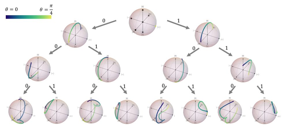
Figure 2: Plotting the LOCC measurement basis for each qubit on a Bloch sphere in a four-qubit system described by Eq. (64) and Eq. (65). The eigenstates of Pauli matrices $\ket{0,1}$, $\ket{\pm}$ and $\ket{L,R}=\frac{\ket{0}\pm i\ket{1}}{\sqrt{2}}$ are labeled on the Bloch sphere. Columns from top to bottom each represent measurement on qubit ${\mathfrak{s}}_{1},{\mathfrak{s}}_{2},{\mathfrak{s}}_{3},{\mathfrak{s}}_{4}$ and arrows represent how the measurement basis should be chosen based on previous measurement results $x=0,1$. The measurement basis is represented by a point on the surface of the Bloch sphere which corresponds to $x=0$. The color indicates the value of Hamiltonian strength $\theta\in[0,\frac{\pi}{4}]$. Note that the measurement on first qubit does not change with time because $M^{{\mathfrak{s}}_{1}}=\mathrm{Tr}_{{\mathfrak{s}}_{2}\ldots{\mathfrak{s}}_{4}}(M)$ and $\mathrm{Tr}_{{\mathfrak{s}}_{2}\ldots{\mathfrak{s}}_{4}}(\ket{\psi_{\theta}}\bra{\psi_{\theta}}-\frac{1}{16}I)$ are always proportional to $\sigma_{z}$.

Appendix E LM is not sufficient to saturate the QCRB for multipartite systems

Here we want to show LM is not sufficient to saturate the QCRB for sufficiently large $n$ in general sensing scenarios, where $n$ is the number of subsystems. Consider Hilbert space $\mathcal{H}^{\otimes n}$ where $\dim\mathcal{H}=d$. For type (i) or (ii) states, let

$$E_{x_{1},\ldots,x_{n}}=E_{x_{1}}^{{\mathfrak{s}}_{1}}\otimes E_{x_{2}}^{{\mathfrak{s}}_{2}}\otimes\cdots\otimes E_{x_{n}}^{{\mathfrak{s}}_{n}},$$ (66)

be a QCRB-saturating local measurement satisfying

$$(E_{x_{1}}^{{\mathfrak{s}}_{1}}\otimes E_{x_{2}}^{{\mathfrak{s}}_{2}}\otimes\cdots\otimes E_{x_{n}}^{{\mathfrak{s}}_{n}})M(E_{x_{1}}^{{\mathfrak{s}}_{1}}\otimes E_{x_{2}}^{{\mathfrak{s}}_{2}}\otimes\cdots\otimes E_{x_{n}}^{{\mathfrak{s}}_{n}})=0,~{}~{}~{}\forall(x_{1},\ldots,x_{n})\in[r_{1}]\times\cdots\times[r_{n}].$$ (67)

where $[r]=\{1,2,\ldots,r\}$. Let $\{\ket{E_{x_{j},i_{j}}^{{\mathfrak{s}}_{j}}}\}_{i_{j}}$ be a basis of the support of $E_{x_{j}}^{{\mathfrak{s}}_{j}}$. Then Eq. (67) implies

$$\mathrm{Tr}\big{(}M(F_{1}^{{\mathfrak{s}}_{1}}\otimes\cdots\otimes F_{n}^{{\mathfrak{s}}_{n}})\big{)}=0,$$ (68)

for all Hermitian $F_{i}^{{\mathfrak{s}}_{i}}\in{\rm span}\{\ket{E_{x_{i},j_{i}}^{{\mathfrak{s}}_{i}}}\bra{E_{x_{i},j_{i}}^{{\mathfrak{s}}_{i}}},\forall x_{i},j_{i}\}$.

We first consider type (i) states, then if we define $\ket{\psi_{\theta}^{\perp}}=(1-\ket{\psi_{\theta}}\bra{\psi_{\theta}})\ket{\partial_{\theta}\psi}$,

$$M=\ket{\psi_{\theta}}\bra{\psi_{\theta}^{\perp}}-\ket{\psi_{\theta}^{\perp}}\bra{\psi_{\theta}}.$$ (69)

Suppose $\mathcal{H}^{\otimes n}=\mathcal{H}_{1}\otimes\mathcal{H}_{2}$ where $\mathcal{H}_{1}=\mathcal{H}^{\otimes m}$ with $m\leq n/2$. Then the reduce matrix $M_{r}=\mathrm{Tr}_{\mathcal{H}_{2}}(M)$ after tracing out $\mathcal{H}_{2}$ could be an arbitrary traceless anti-Hermitian matrix (up a real factor) by choosing

$$\ket{\psi_{\theta}}=\frac{1}{\sqrt{d^{m}}}\sum_{i=1}^{d^{m}}\ket{i}_{\mathcal{H}_{1}}\ket{i}_{\mathcal{H}_{2}},$$ (70)

$$\ket{\psi_{\theta}^{\perp}}=\frac{1}{\sqrt{\mathrm{Tr}(-M_{r}^{2})}}\sum_{i,j=1}^{d^{m}}M_{r,ij}\ket{i}_{\mathcal{H}_{1}}\ket{j}_{\mathcal{H}_{2}}.$$ (71)

According to Eq. (68), $M_{r}$ has to satisfy

$$\mathrm{Tr}\big{(}M_{r}(F_{1}^{{\mathfrak{s}}_{1}}\otimes\cdots\otimes F_{m}^{{\mathfrak{s}}_{n}})\big{)}=0,$$ (72)

for all Hermitian $F_{i}^{{\mathfrak{s}}_{i}}\in{\rm span}\{\ket{E_{x_{i},j_{i}}^{{\mathfrak{s}}_{i}}}\bra{E_{x_{i},j_{i}}^{{\mathfrak{s}}_{i}}},\forall x_{i},j_{i}\}$. There must exists a (not necessarily orthonormal) basis $\{\ket{e_{i}^{\mathfrak{s}_{k}}}\}_{i=1}^{d}$ for each $k$ such that

$$\bigg{(}\bigotimes_{k=1}^{m}\bra{e_{k_{i}}^{\mathfrak{s}_{k}}}\bigg{)}M_{r}\bigg{(}\bigotimes_{k=1}^{m}\ket{e_{i_{k}}^{\mathfrak{s}_{k}}}\bigg{)}=0,\quad\forall i_{k}=1,2,\ldots,d.$$ (73)

Note that the degree of freedom of an arbitrary traceless anti-Hermitian matrix $M_{r}$ is $d^{2m}-1$. But the degree of freedom for matrices satisfying Eq. (73) is at most $d^{2m}-d^{m}+md^{4}$ which is smaller than $d^{2m}$ for large enough $m$. Here $d^{m}$ is the minimum number of equations of constraints in Eq. (73) and $md^{4}$ is the local freedoms in choosing the basis. Therefore Eq. (73) could not be satisfied for arbitrary $M_{r}$, implying that Eq. (68) could not be satisfied for all possible $M$. For type (ii) states, the same argument holds if we replace $\ket{\psi_{\theta}}$ and $\ket{\psi_{\theta}^{\perp}}$ above with $\ket{\psi_{0}}$ and $\ket{\psi_{1}}$.

Appendix F Eq. (26) cannot be distinguished using LM

Consider a two-qubit system. Here we show that

$$\ket{\psi_{\theta}}=\frac{1}{\sqrt{2}}(\ket{00}+\ket{1+}),\quad\ket{\psi_{\theta}^{\perp}}=\frac{1}{\sqrt{2}}(\ket{01}+\ket{1-})$$ (74)

cannot be distinguished using LM, i.e. there is no LM $\{E_{x_{1}}^{\mathfrak{s}_{1}}\otimes E_{x_{2}}^{\mathfrak{s}_{2}}\}$ such that

$$\bra{\psi_{\theta}}E_{x_{1}}^{\mathfrak{s}_{1}}\otimes E_{x_{2}}^{\mathfrak{s}_{2}}\ket{\psi_{\theta}}\cdot\bra{\psi_{\theta}^{\perp}}E_{x_{1}}^{\mathfrak{s}_{1}}\otimes E_{x_{2}}^{\mathfrak{s}_{2}}\ket{\psi_{\theta}^{\perp}}=0,\quad\forall x_{1},x_{2}.$$ (75)

Choose $\ket{\phi_{1}}$ and $\ket{\phi_{2}}$ in the support of some $E_{x_{1}}^{\mathfrak{s}_{1}}$ and $E_{x_{2}}^{\mathfrak{s}_{2}}$ respectively. Then

$$\braket{\psi_{\theta}}{\phi_{1}\otimes\phi_{2}}\braket{\phi_{1}\otimes\phi_{2}}{\psi_{\theta}^{\perp}}=0.$$ (76)

Since the identity operator $I$ is in the span of all $\ket{\phi_{2}}\bra{\phi_{2}}$, we must have

$$\braket{\psi_{\theta}}{\phi_{1}}\braket{\phi_{1}}{\psi_{\theta}^{\perp}}=0.$$ (77)

Note that both $\braket{\phi_{1}}{\psi_{\theta}}$ and $\braket{\phi_{1}}{\psi_{\theta}^{\perp}}$ are not zero because $\ket{\psi_{\theta}}$ and $\ket{\psi_{\theta}^{\perp}}$ are entangled. Let $\ket{e^{(2)}_{1}}\propto\braket{\phi_{1}}{\psi_{\theta}}$ and $\ket{e^{(2)}_{2}}\propto\braket{\phi_{1}}{\psi_{\theta}^{\perp}}$ be unit vectors. We must have either $\ket{\phi_{2}}=\ket{e^{(2)}_{1}}$ or $\ket{\phi_{2}}=\ket{e^{(2)}_{2}}$ because $\braket{e^{(2)}_{1}}{\phi_{2}}\braket{\phi_{2}}{e^{(2)}_{2}}=0$. Therefore, there are two orthonormal basis $\ket{e^{(1,2)}_{1,2}}$ such that

$$\braket{e_{i}^{(1)}\otimes e_{j}^{(2)}}{\psi_{\theta}}\braket{\psi_{\theta}^{\perp}}{e_{i}^{(1)}\otimes e_{j}^{(2)}}=0,\quad\forall i,j=1,2.$$ (78)

Since $\ket{\psi_{\theta}}$ and $\ket{\psi_{\theta}^{\perp}}$ are both entangled, we must have

$$\ket{\psi_{\theta}}=\lambda_{1}\ket{e_{1}^{(1)}}\ket{e_{1}^{(2)}}+\lambda_{2}\ket{e_{2}^{(1)}}\ket{e_{2}^{(2)}},\;\ket{\psi_{\theta}}=\mu_{1}\ket{e_{1}^{(1)}}\ket{e_{2}^{(2)}}+\mu_{2}\ket{e_{2}^{(1)}}\ket{e_{1}^{(2)}},$$ (79)

for some non-zero $\lambda_{1,2}$ and $\mu_{1,2}$. Clearly, Eq. (26) does not have this form. Therefore, they cannot be distinguished using LM.

On the other hand, there exists an LM such that the QCRB is saturated. For example,

$$\ket{E_{1}^{\mathfrak{s}_{1}}}=\ket{0},\quad\ket{E_{2}^{\mathfrak{s}_{1}}}=\ket{1},$$ (80)

$$\ket{E_{1}^{\mathfrak{s}_{2}}}=\cos\frac{\pi}{8}\ket{0}+\sin\frac{\pi}{8}\ket{1},\quad\ket{E_{2}^{\mathfrak{s}_{2}}}=-\sin\frac{\pi}{8}\ket{0}+\cos\frac{\pi}{8}\ket{1}.$$ (81)

Appendix G There is no QCRB-saturating projective LM for Eq. (27)

Here we prove there is no QCRB-saturating projective LM when

$$A=\begin{pmatrix}{\sqrt{2}}/{2}&0&0\\ 0&{1}/{2}&0\\ 0&0&1/2\\ \end{pmatrix},\;B=\begin{pmatrix}{\sqrt{2}i}/{2}&0&0\\ 0&{-i}/{2}&0\\ 0&0&{-i}/{2}\\ \end{pmatrix}$$ (82)

but there is a QCRB-saturating general LM. From the proof of Lemma 2, we can see that it is equivalent to the statement that there are no unitaries $U$ and $V$ such that Eq. (22) and Eq. (23) are both satisfied, but there are isometries $U$ and $V$ such that these conditions are satisfied.

Our goal is to prove there are no unitaries $U$ and $V$ such that Eq. (22) is satisfied. Now suppose $U$ and $V$ are unitary. According to the definitions of $C$ and $D$, we have

$$C_{ij}=(U^{\dagger}AV)_{ij}=\frac{1}{2}\big{(}\sqrt{2}\overline{U}_{1i}V_{1j}+\overline{U}_{2i}V_{2j}+\overline{U}_{3i}V_{3j}\big{)},$$ (83)

$$D_{ij}=(U^{\dagger}BV)_{ij}=\frac{1}{2}\big{(}\sqrt{2}i\overline{U}_{1i}V_{1j}-i\overline{U}_{2i}V_{2j}-i\overline{U}_{3i}V_{3j}\big{)},$$ (84)

and

$$\begin{split}C_{ij}\overline{D}_{ij}-D_{ij}\overline{C}_{ij}&=\frac{1}{4}(\sqrt{2}\overline{U}_{1i}V_{1j}+\overline{U}_{2i}V_{2j}+U_{i3}v_{3j})(-\sqrt{2}iU_{1i}\overline{V}_{1j}+iU_{2i}\overline{V}_{2j}+iU_{3i}\overline{V}_{3j})\\ &\qquad-(\sqrt{2}U_{1i}\overline{V}_{1j}+U_{2i}\overline{V}_{2j}+U_{3i}\overline{V}_{3j})(\sqrt{2}i\overline{U}_{1i}V_{1j}-i\overline{U}_{2i}V_{2j}-i\overline{U}_{3i}V_{3j})\\ &=-i\left|\overline{U}_{1i}V_{1j}\right|^{2}+\frac{i}{2}\left|\overline{U}_{2i}V_{2j}+\overline{U}_{3i}V_{3j}\right|^{2}=0,\quad\forall i,j.\end{split}$$ (85)

First note that the following two transformations do not change Eq. (22):

1. $U\rightarrow\begin{pmatrix}1&0\\ 0&R\\ \end{pmatrix}U,\;V\rightarrow\begin{pmatrix}1&0\\ 0&R\\ \end{pmatrix}V,$ where $R$ is any unitary matrix in ${\mathbb{C}}^{2\times 2}$.

2. $U\rightarrow UD_{1},\;V\rightarrow VD_{2},$ where $D_{1}$ and $D_{2}$ are arbitrary diagonal unitary matrices.

Therefore, WLOG, we assume $(U_{11},U_{21},U_{31})=(\mathbb{R}_{+},\mathbb{R}_{+},0)$.

$$2\left|\overline{U}_{11}V_{1j}\right|^{2}=\left|\overline{U}_{21}V_{2j}\right|^{2},\quad\forall j,$$ (86)

$$\Rightarrow~{}~{}2\left|U_{11}\right|^{2}\sum_{j=1}^{3}\left|V_{1j}\right|^{2}=\left|U_{21}\right|^{2}\sum_{j=1}^{3}\left|V_{2j}\right|^{2},$$ (87)

$$\Rightarrow~{}~{}U_{11}=1/\sqrt{3},\;U_{21}=\sqrt{2}/\sqrt{3},\text{~{}~{}and~{}~{}}\left|V_{1j}\right|^{2}=\left|V_{2j}\right|^{2}=:s_{j},\quad\forall j.$$ (88)

WLOG, assume $V_{2j}=\sqrt{s_{j}}$, $\forall j$.

Consider the following two situations:

Situation (1): $s_{j}=0$ for some $j$. Then $\left|\overline{U}_{3i}V_{3j}\right|^{2}=0$ and $U_{3i}=0$ for all $i$, which is not possible.

Situation (2): $s_{j}>0$, $\forall j$. Then for $i\neq 1$,

$$2\left|\overline{U}_{1i}V_{1j}\right|^{2}=\left|\overline{U}_{2i}V_{2j}+\overline{U}_{3i}V_{3j}\right|^{2},\forall j,$$ (89)

$$\Rightarrow~{}~{}2\left|U_{1i}\right|^{2}=\left|U_{2i}\right|^{2}+\left|U_{3i}\right|^{2}\frac{1}{s_{j}}\left|V_{3j}\right|^{2}+\frac{2}{\sqrt{s_{j}}}\cdot{\mathrm{Re}}[U_{2i}\overline{U}_{3i}V_{3j}],$$ (90)

$$\Rightarrow~{}~{}2\sum_{i>1}\left|U_{1i}\right|^{2}=\sum_{i>1}\left|U_{2i}\right|^{2}+\sum_{i>1}\left|U_{3i}\right|^{2}\frac{1}{s_{j}}\left|V_{3j}\right|^{2},$$ (91)

$$\Rightarrow~{}~{}\left|V_{1j}\right|^{2}=\left|V_{2j}\right|^{2}=\left|V_{3j}\right|^{2}=1/3.$$ (92)

According to Eq. (90), for some $i\neq 1$ such that $U_{2i}\overline{U}_{3i}$,

$${\mathrm{Re}}[U_{2i}\overline{U}_{3i}V_{31}]={\mathrm{Re}}[U_{2i}\overline{U}_{3i}V_{32}]={\mathrm{Re}}[U_{2i}\overline{U}_{3i}V_{33}].$$ (93)

We must have $V_{3i}\in\{e^{i\theta_{1}}/\sqrt{3},e^{i\theta_{2}}/\sqrt{3}\}$ for all $i$. This is not possible because in that case

$$\sum_{i=1}^{3}\overline{V}_{3i}V_{2i}\neq 0,$$ (94)

contradicting with the requirement that $V$ is unitary.

On the other hand, let

$$U=\begin{pmatrix}1/\sqrt{3}&1/\sqrt{3}&1/\sqrt{3}\\ \sqrt{2}/\sqrt{3}&-1/\sqrt{6}&-1/\sqrt{6}\\ 0&-i/\sqrt{2}&i/\sqrt{2}\\ \end{pmatrix},\quad V=\begin{pmatrix}e^{i\pi/4}/2&e^{i3\pi/4}/2&-e^{i\pi/4}/2&-e^{i3\pi/4}/2\\ 1/2&1/2&1/2&1/2\\ 1/2&-1/2&1/2&-1/2\\ \end{pmatrix},$$ (95)

one can verify in this case both Eq. (22) and Eq. (23) are satisfied.

References

• Giovannetti et al. (2006) V. Giovannetti, S. Lloyd,  and L. Maccone, Physical Review Letters 96, 010401 (2006).
• Giovannetti et al. (2011) V. Giovannetti, S. Lloyd,  and L. Maccone, Nature Photonics 5, 222 (2011).
• Degen et al. (2017) C. L. Degen, F. Reinhard,  and P. Cappellaro, Review Modern Physics 89, 035002 (2017).
• Braun et al. (2018) D. Braun, G. Adesso, F. Benatti, R. Floreanini, U. Marzolino, M. W. Mitchell,  and S. Pirandola, Review Modern Physics 90, 035006 (2018).
• Pezzè et al. (2018) L. Pezzè, A. Smerzi, M. K. Oberthaler, R. Schmied,  and P. Treutlein, Review Modern Physics 90, 035005 (2018).
• Pirandola et al. (2018) S. Pirandola, B. R. Bardhan, T. Gehring, C. Weedbrook,  and S. Lloyd, Nature Photonics 12, 724 (2018).
• Sanders and Milburn (1995) B. Sanders and G. Milburn, Physical Review Letters 75, 2944 (1995).
• Bollinger et al. (1996) J. Bollinger, W. M. Itano, D. Wineland,  and D. Heinzen, Physical Review A 54, R4649 (1996).
• Huelga et al. (1997) S. F. Huelga, C. Macchiavello, T. Pellizzari, A. K. Ekert, M. B. Plenio,  and J. I. Cirac, Physical Review Letters 79, 3865 (1997).
• Leibfried et al. (2004) D. Leibfried, M. Barrett, T. Schaetz, J. Britton, J. Chiaverini, W. Itano, J. Jost, C. Langer,  and D. Wineland, Science 304, 1476 (2004).
• Giovannetti et al. (2004) V. Giovannetti, S. Lloyd,  and L. Maccone, Science 306, 1330 (2004).
• Bu$\mathbf{z}$ek et al. (1999) V. Bu$\mathbf{z}$ek, R. Derka,  and S. Massar, Physical Review Letters 82, 2207 (1999).
• Valencia et al. (2004) A. Valencia, G. Scarcelli,  and Y. Shih, Applied Physics Letters 85, 2655 (2004).
• de Burgh and Bartlett (2005) M. de Burgh and S. D. Bartlett, Physical Review A 72, 042301 (2005).
• Caves (1981) C. M. Caves, Physical Review D 23, 1693 (1981).
• Yurke et al. (1986) B. Yurke, S. L. McCall,  and J. R. Klauder, Physical Review A 33, 4033 (1986).
• Berry and Wiseman (2000) D. Berry and H. Wiseman, Physical Review Letters 85, 5098 (2000).
• Higgins et al. (2007) B. L. Higgins, D. W. Berry, S. D. Bartlett, H. M. Wiseman,  and G. J. Pryde, Nature 450, 393 (2007).
• Helstrom (1976) C. W. Helstrom, Quantum detection and estimation theory (Academic press, 1976).
• Helstrom (1968) C. Helstrom, IEEE Transactions on Information Theory 14, 234 (1968).
• Paris (2009) M. G. Paris, International Journal of Quantum Information 7, 125 (2009).
• Braunstein and Caves (1994) S. L. Braunstein and C. M. Caves, Physical Review Letters 72, 3439 (1994).
• Kobayashi et al. (2011) H. Kobayashi, B. L. Mark,  and W. Turin, Signal Processing, Queueing Theory and Mathematical Finance  (2011).
• Casella and Berger (2002) G. Casella and R. L. Berger, Statistical inference, Vol. 2 (Duxbury Pacific Grove, CA, 2002).
• Lehmann and Casella (2006) E. L. Lehmann and G. Casella, Theory of point estimation (Springer Science & Business Media, 2006).
• Brody and Hughston (1996) D. C. Brody and L. P. Hughston, Physical Review Letters 77, 2851 (1996).
• Fujiwara (2006) A. Fujiwara, Journal of Physics A Mathematical General 39, 12489 (2006).
• Barndorff-Nielsen and Gill (2000) O. Barndorff-Nielsen and R. Gill, Journal of Physics A: Mathematical and General 33, 4481 (2000).
• Hayashi (2011) M. Hayashi, Communications in Mathematical Physics 304, 689 (2011).
• Yang et al. (2019a) Y. Yang, G. Chiribella,  and M. Hayashi, Communications in Mathematical Physics 368, 223 (2019a).
• Gill (2008) R. D. Gill, in Quantum Stochastics and Information: Statistics, Filtering and Control (World Scientific, 2008) pp. 239–261.
• Pezze and Smerzi (2014) L. Pezze and A. Smerzi, arXiv:1411.5164  (2014).
• Jarzyna and Demkowicz-Dobrzański (2015) M. Jarzyna and R. Demkowicz-Dobrzański, New Journal of Physics 17, 013010 (2015).
• Górecki et al. (2020) W. Górecki, R. Demkowicz-Dobrzański, H. M. Wiseman,  and D. W. Berry, Physical Review Letters 124, 030501 (2020).
• Friis et al. (2017) N. Friis, D. Orsucci, M. Skotiniotis, P. Sekatski, V. Dunjko, H. J. Briegel,  and W. Dür, New Journal of Physics 19, 063044 (2017).
• Boixo et al. (2008) S. Boixo, A. Datta, S. T. Flammia, A. Shaji, E. Bagan,  and C. M. Caves, Physical Review A 77, 012317 (2008).
• Roy and Braunstein (2008) S. Roy and S. L. Braunstein, Physical Review Letters 100, 220501 (2008).
• Rams et al. (2018) M. M. Rams, P. Sierant, O. Dutta, P. Horodecki,  and J. Zakrzewski, Physical Review X 8, 021022 (2018).
• Chitambar et al. (2014) E. Chitambar, D. Leung, L. Man$\mathbf{c}$inska, M. Ozols,  and A. Winter, Communications in Mathematical Physics 328, 303 (2014).
• Cirac et al. (1999) J. Cirac, A. Ekert, S. Huelga,  and C. Macchiavello, Physical Review A 59, 4249 (1999).
• Raussendorf and Briegel (2001) R. Raussendorf and H. J. Briegel, Physical Review Letters 86, 5188 (2001).
• DiVincenzo et al. (2002) D. P. DiVincenzo, D. W. Leung,  and B. M. Terhal, IEEE Transactions on Information Theory 48, 580 (2002).
• Verstraete and Cirac (2003) F. Verstraete and J. I. Cirac, Physical Review Letters 91, 010404 (2003).
• Kalb et al. (2017) N. Kalb, A. A. Reiserer, P. C. Humphreys, J. J. W. Bakermans, S. J. Kamerling, N. H. Nickerson, S. C. Benjamin, D. J. Twitchen, M. Markham,  and R. Hanson, Science 356, 928 (2017).
• Chou et al. (2018) K. S. Chou, J. Z. Blumoff, C. S. Wang, P. C. Reinhold, C. J. Axline, Y. Y. Gao, L. Frunzio, M. Devoret, L. Jiang,  and R. Schoelkopf, Nature 561, 368 (2018).
• Bernien et al. (2017) H. Bernien, S. Schwartz, A. Keesling, H. Levine, A. Omran, H. Pichler, S. Choi, A. S. Zibrov, M. Endres, M. Greiner, et al., Nature 551, 579 (2017).
• Zhang et al. (2017) J. Zhang, G. Pagano, P. W. Hess, A. Kyprianidis, P. Becker, H. Kaplan, A. V. Gorshkov, Z.-X. Gong,  and C. Monroe, Nature 551, 601 (2017).
• Bagan et al. (2004) E. Bagan, M. Baig, R. Muñoz-Tapia,  and A. Rodriguez, Physical Review A 69, 010304 (2004).
• Bagan et al. (2006) E. Bagan, M. Ballester, R. Gill, R. Muñoz-Tapia,  and O. Romero-Isart, Physical Review Letters 97, 130501 (2006).
• Calsamiglia et al. (2010) J. Calsamiglia, J. de Vicente, R. Muñoz-Tapia,  and E. Bagan, Physical Review Letters 105, 080504 (2010).
• Ghosh et al. (2001) S. Ghosh, G. Kar, A. Roy, A. Sen, U. Sen, et al., Physical Review Letters 87, 277902 (2001).
• Walgate et al. (2000) J. Walgate, A. J. Short, L. Hardy,  and V. Vedral, Physical Review Letters 85, 4972 (2000).
• Acín et al. (2000) A. Acín, R. Tarrach,  and G. Vidal, Physical Review A 61, 062307 (2000).
• Bagan et al. (2005) E. Bagan, M. Ballester, R. Munoz-Tapia,  and O. Romero-Isart, Physical Review Letters 95, 110504 (2005).
• Duan et al. (2007) R. Duan, Y. Feng, Z. Ji,  and M. Ying, Physical Review Letters 98, 230502 (2007).
• Yu et al. (2011) N. Yu, R. Duan,  and M. Ying, Physical Review A 84, 012304 (2011).
• Hayashi et al. (2006) M. Hayashi, D. Markham, M. Murao, M. Owari,  and S. Virmani, Physical Review Letters 96, 040501 (2006).
• Zhu and Hayashi (2018) H. Zhu and M. Hayashi, Physical Review Letters 120, 030404 (2018).
• De Pasquale et al. (2016) A. De Pasquale, D. Rossini, R. Fazio,  and V. Giovannetti, Nature Communications 7, 12782 (2016).
• Sone et al. (2018) A. Sone, Q. Zhuang,  and P. Cappellaro, Physical Review A 98, 012115 (2018).
• Sone et al. (2019) A. Sone, Q. Zhuang, C. Li, Y.-X. Liu,  and P. Cappellaro, Physical Review A 99, 052318 (2019).
• Venuti and Zanardi (2007) L. C. Venuti and P. Zanardi, Physical Review Letters 99, 095701 (2007).
• Tamascelli et al. (2016) D. Tamascelli, C. Benedetti, S. Olivares,  and M. G. Paris, Physical Review A 94, 042129 (2016).
• Hauke et al. (2016) P. Hauke, M. Heyl, L. Tagliacozzo,  and P. Zoller, Nature Physics 12, 778 (2016).
• Zhang et al. (2018) Y.-R. Zhang, Y. Zeng, H. Fan, J. You,  and F. Nori, Physical Review Letters 120, 250501 (2018).
• Yang et al. (2019b) J. Yang, S. Pang, Y. Zhou,  and A. N. Jordan, Physical Review A 100, 032104 (2019b).
• Matsumoto (2002) K. Matsumoto, Journal of Physics A: Mathematical and General 35, 3111 (2002).
• Ragy et al. (2016) S. Ragy, M. Jarzyna,  and R. Demkowicz-Dobrzański, Physical Review A 94, 052108 (2016).
• Baumgratz and Datta (2016) T. Baumgratz and A. Datta, Physical Review Letters 116, 030801 (2016).
• Yuan (2016) H. Yuan, Physical Review Letters 117, 160801 (2016).
• Proctor et al. (2018) T. J. Proctor, P. A. Knott,  and J. A. Dunningham, Physical Review Letters 120, 080501 (2018).
• Ge et al. (2018) W. Ge, K. Jacobs, Z. Eldredge, A. V. Gorshkov,  and M. Foss-Feig, Physical Review Letters 121, 043604 (2018).
• Qian et al. (2019) K. Qian, Z. Eldredge, W. Ge, G. Pagano, C. Monroe, J. V. Porto,  and A. V. Gorshkov, Phys. Rev. A 100, 042304 (2019).
• Viola et al. (1999) L. Viola, E. Knill,  and S. Lloyd, Physical Review Letters 82, 2417 (1999).
• Uhrig (2007) G. S. Uhrig, Physical Review Letters 98, 100504 (2007).
• Biercuk et al. (2009) M. J. Biercuk, H. Uys, A. P. VanDevender, N. Shiga, W. M. Itano,  and J. J. Bollinger, Nature 458, 996 (2009).
• Kessler et al. (2014) E. M. Kessler, I. Lovchinsky, A. O. Sushkov,  and M. D. Lukin, Physical Review Letters 112, 150802 (2014).
• Dür et al. (2014) W. Dür, M. Skotiniotis, F. Froewis,  and B. Kraus, Physical Review Letters 112, 080801 (2014).
• Arrad et al. (2014) G. Arrad, Y. Vinkler, D. Aharonov,  and A. Retzker, Physical Review Letters 112, 150801 (2014).
• Zhou et al. (2018) S. Zhou, M. Zhang, J. Preskill,  and L. Jiang, Nature Communications 9, 78 (2018).
• Demkowicz-Dobrzański et al. (2017) R. Demkowicz-Dobrzański, J. Czajkowski,  and P. Sekatski, Physical Review X 7, 041009 (2017).
• Reiter et al. (2017) F. Reiter, A. S. Sørensen, P. Zoller,  and C. Muschik, Nature Communications 8, 1822 (2017).