Control Variables, Discrete Instruments, and Identification of Structural Functions

Abstract

Control variables provide an important means of controlling for endogeneity in econometric models with nonseparable and/or multidimensional heterogeneity. We allow for discrete instruments, giving identification results under a variety of restrictions on the way the endogenous variable and the control variables affect the outcome. We consider many structural objects of interest, such as average or quantile treatment effects. We illustrate our results with an empirical application to Engel curve estimation.

Keywords: Control variables, discrete instruments, structural functions, endogeneity, partially nonparametric, nonseparable models, identification, treatment effects.

JEL classification: C14, C31, C35

1 Introduction

Nonseparable and/or multidimensional heterogeneity is important. It is present in discrete choice models as in McFadden (1973) and Hausman and Wise (1978). Multidimensional heterogeneity in demand functions allows price and income elasticities to vary over individuals in unrestricted ways, e.g., Hausman and Newey (2016) and Kitamura and Stoye (2018). It allows general variation in production technologies. Treatment effects that vary across individuals require intercept and slope heterogeneity.

Endogeneity is often a problem in these models because we are interested in the effect of an observed choice, or treatment variable on an outcome. Control variables provide an important means of controlling for endogeneity with multidimensional heterogeneity. A control variable is an observed or estimable variable that makes heterogeneity and treatment independent when it is conditioned on. Observed covariates serve as control variables for treatment effects (Rosenbaum and Rubin, 1983). The conditional cumulative distribution function (CDF) of a choice variable given an instrument can serve as a control variable in economic models (Imbens and Newey, 2009).

Nonparametric identification of many objects of interest, such as average or quantile treatment effects, requires a full support condition, that the support of the control variable conditional on the treatment variable is equal to the marginal support of the control variable. This restriction is often not satisfied in practice; e.g., see Imbens and Newey (2009) for Engel curves. It cannot be satisfied when instruments are discrete. One approach to this problem is to focus on identified sets for objects of interest, as for quantile effect in Imbens and Newey (2009). Another approach is to consider restrictions on the model that allow for point identification. Florens et al. (2008) did so by showing identification when the structural function is a polynomial in the endogenous variable and a measurable separability condition is satisfied. Torgovitsky (2015) and D’Haultfœuille and Février (2015) did so by showing identification for discrete instruments when the structural disturbance is a scalar.

In this paper we give identification results under a variety of restrictions on the way the treatment and control variables enter the control regression of the outcome of interest on the endogenous and control variables. The control regression functions (CRF) we consider are the conditional mean, quantile, and (monotone transformations of) distribution functions of the outcome given the endogenous and control variables. We give identification results when a CRF is a linear combinations of known functions of a treatment and control variables. We also give identification results for partially nonparametric specifications where a CRF is a linear combination of known functions of either the treatment or the control variables, with coefficients that are unknown functions of the other variable.

The partially nonparametric specifications we consider generalise those of Florens et al. (2008) to allow for nonpolynomial functions of endogenous variables or control variables and to consider CRFs other than the mean. We also take a different approach to identification, focusing here on conditional nonsingularity of second moment matrices instead of measurable separability. These results here also generalise the identification conditions for the baseline models considered by Chernozhukov et al. (2017). For triangular systems with a continuous treatment, our identification results also generalise those of Masten and Torgovitsky (2016) to allow for known functions of control variables, and to include quantile and distribution treatment effects. For treatment effects with a binary or discrete treatment, the present paper contributes to the literature (Rosenbaum and Rubin, 1983; Imbens, 2000; Wooldridge, 2004) by providing conditions based on conditional nonsingularity for identification of average treatment effects. These results complement those of Newey and Stouli (2018) by allowing for known functions of control variables and by considering conditional quantile and distribution CRFs.

A main benefit of our approach is that it allows for discrete instruments. For triangular systems, with continuous treatment, we show identification of average, distribution, and quantile treatment effects given sufficient variation in the discrete instrument conditional on the endogenous variable. These results are obtained by viewing various control regression specifications as varying coefficient models. These results generalise the analysis of Masten and Torgovitsky (2016) to conditional distribution and quantile effects, and to known functions of control variables.

These results provide an alternative approach to identifying objects of interest in nonseparable models with discrete instruments. Instead of restricting the dimension of the heterogeneity to obtain identification with discrete instruments as done in Torgovitsky (2015) and D’Haultfœuille and Février (2015), we can allow for multidimensional heterogeneity but restrict the way the treatment or controls affect the outcome.

These results provide an alternative approach to identifying treatment effects with a finite number of treatment regimes. Here the CRF depends on treatment only through the (known) vector of dummy variables for each regime. Nonsingularity of the conditional second moment matrix provides a relatively simple and general condition for identification of treatment effects. If restrictions are placed on the way the control variables affect the CRF then the conditional nonsingularity condition can be weakened. For example for a binary treatment regime (i.e., treated or not) we can allow for the propensity score to be bounded away from zero and one only on a subset of control variables values.

We illustrate our results using an empirical application to Engel curves estimation using British expenditure survey data. We find that estimates of average, distributional and quantile treatment effects of total expenditure on food and leisure expenditure are not very sensitive to discretisation of the income instruments. We find that as we “coarsen” the instrument by only using knowledge of income intervals the structural estimates do not change much until the instrument is very coarse. Thus, in this empirical example we find that one can obtain good structural estimates even with discrete instruments.

In Section 2 we introduce the parametric models we consider. In Section 3 we give identification results. In Section 4 we extend these results to partially nonparametric models that allow for nonparametric components. Section 5 reports the results of an empirical application to Engel curve estimation.

2 Parametric Modelling of Control Regressions

Let $Y$ denote an outcome variable of interest and $X$ an endogenous treatment with supports denoted by $\mathcal{Y}$ and $\mathcal{X}$, respectively. For $\varepsilon$ a structural disturbance vector of unknown dimension, a nonseparable control variable model takes the form

$$Y=g(X,\varepsilon),$$ (2.1)

where $X$ and $\varepsilon$ are independent conditional on an observable or estimable control variable denoted $V$. Conditioning on the control variable allows to identify general features of the structural relationship between $X$ and $Y$ in model (2.1), such as those captured by the structural functions of Blundell and Powell (2003, 2004), and Imbens and Newey (2009). An important kind of model where $X$ is independent of $\varepsilon$ conditional on $V$ is a structural triangular system where $X=h(Z,\eta)$ and $h(z,\eta)$ is one-to-one in $\eta$. If $(\varepsilon,\eta)$ are jointly independent of $Z$ then $V=F_{X\mid Z}(X\mid Z)$, the conditional CDF of $X$ given $Z$, is a control variable in this model (Imbens and Newey, 2009).

Leading examples of structural functions are the average structural function, $\mu(x)$, the distribution structural function, $G(y,x)$, and the quantile structural function (QSF) $Q(p,x)$, given by

$$\mu(x) := \int g(x,\varepsilon)F_{\varepsilon}(d\varepsilon),\quad G(y,x):=\text{Pr}(g(x,\varepsilon)\leq y),$$

$$Q(p,x) := p^{\text{th}}\text{ quantile of }g(x,\varepsilon),$$

where $x$ is fixed in these expressions. These structural functions may be identifiable from control regressions of $Y$ on $X$ and $V$, including the conditional mean $E[Y\mid X,V],$ CDF, $F_{Y\mid XV}(Y\mid X,V)$, and quantile function, $Q_{Y\mid XV}(U\mid X,V)$, of $Y$ given $(X,V)$. In particular, when the support $\mathcal{V}_{x}$ of $V$ conditional on $X=x$ equals the marginal support $\mathcal{V}$ of $V$ we have

$$\mu(x) =\int_{\mathcal{V}}E[Y\mid X=x,V=v]F_{V}(dv),\quad G(y,x)=\int_{\mathcal{V}}F_{Y\mid XV}(y\mid x,v)F_{V}(dv),$$

$$Q(p,x) =G^{\leftarrow}(p,x):=\inf\{y\in\mathbb{R}:G(y,x)\geq p\};$$ (2.2)

see Blundell and Powell (2003) and Imbens and Newey (2009).

The key condition for equation (2.2) is full support, that the support $\mathcal{V}_{x}$ of $V$ conditional on $X=x$ equals the marginal support of $V$. Without full support the integrals would not be well defined because integration would be over a range of $(x,v)$ values that are outside the joint support of $(X,V).$ Having a full support for each $x$ is equivalent to $(X,V)$ having rectangular support. In the absence of a rectangular support, global identification of the structural functions at all $x$ must rely on alternative conditions that identify $F_{Y\mid XV}(y\mid x,v)$ for all $(x,v)\in\mathcal{X}\times\mathcal{V}$ and not merely over the joint support $\mathcal{X}\mathcal{V}$ of $(X,V)$. An example of such conditions are functional form restrictions on the controlled regressions $F_{Y\mid XV}$ and $Q_{Y\mid XV}$ which thus constitute natural modelling targets in the context of nonseparable conditional independence models. Imbens and Newey (2009) did show that structural effects may be partially identified without the full support condition. Here we focus on achieving identification via restricting the form of control regressions.

We begin with parametric specifications that are linear combinations of a vector of known functions $w(X,V)$ having the kronecker product form $p(X)\otimes q(V),$ where $p(X)$ and $q(V)$ are vectors of transformations of $X$ and $V$, respectively. Let $\Gamma$ denote a strictly increasing continuous CDF, such as the Gaussian CDF $\Phi$, with inverse function denoted $\Gamma^{-1}.$ The control regression specifications we consider are

$$E[Y|X,V]=\beta_{0}^{\prime}[p(X)\otimes q(V)],\;\;F_{Y|XV}(y|X,V)=\Gamma(\beta(y)^{\prime}[p(X)\otimes q(V)]),$$ (2.3)

and, when $Y$ is continuous,

$$Q_{Y|X,V}(u|X,V)=\beta(u)^{\prime}[p(X)\otimes q(V)],\quad u\in(0,1),$$ (2.4)

where the coefficients $\beta(y)$ and $\beta(u)$ are functions of $y$ and $u$, respectively. The quantile and conditional mean coefficients are related by $\beta_{0}=\int_{0}^{1}\beta(u)du.$ When $Y$ is discrete, the conditional distribution specification can be thought of as a discrete choice model as in McFadden (1973). Examples of structural models that give rise to CRFs of the form (2.3)-(2.4) are given below and in Chernozhukov et al. (2017).

It is convenient in what follows to use a common notation for the conditional mean, distribution, and quantile control regressions. For $\mathcal{U}=(0,1)$ and an index set $\mathcal{T}=\{0\}$, $\mathcal{Y}$, or $\mathcal{U}$, we define the collection of functions indexed by $\tau\in\mathcal{T}$,

$$\varphi_{\tau}(x,v)=\begin{cases}E[Y\mid X=x,V=v]&\textrm{if $\mathcal{T}$=\{0\}}\\ \Gamma^{-1}\left(F_{Y\mid XV}(\tau\mid x,v)\right)&\textrm{if $\mathcal{T}$=$\mathcal{Y}$}\\ Q_{Y\mid XV}(\tau\mid x,v)&\textrm{if $\mathcal{T}$=$\mathcal{U}$}\end{cases}.$$

While the coefficients $y\mapsto\beta(y)$ and $u\mapsto\beta(u)$ in (2.4) are infinite-dimensional parameters, for each $\tau$ in $\mathcal{T}$ the three control regression specifications share the essentially parametric form

$$\varphi_{\tau}(X,V)=\beta_{\tau}^{\prime}w(X,V),\quad w(X,V):=p(X)\otimes q(V),$$

where the coefficient $\beta_{\tau}$ is a finite-dimensional parameter vector. This interpretation motivates the following definition of a parametric class of conditional independence models.

Assumption 1.

(a) For the model in (2.1), there exists a control variable $V$ such that $X$ and $\varepsilon$ are independent conditional on $V$. (b) For a specified set $\mathcal{T}=\{0\}$, $\mathcal{Y}$, or $\mathcal{U}$, and each $\tau\in\mathcal{T}$, the outcome $Y$ conditional on $(X,V)$ follows the model

$$\varphi_{\tau}(X,V)=\beta_{\tau}^{\prime}w(X,V),\quad w(X,V):=p(X)\otimes q(V).$$ (2.5)

Standard results such as those of Newey and McFadden (1994) imply that point identification of $\beta_{\tau}$ only requires positive definiteness of the second moment matrix $E[w(X,V)w(X,V)^{\prime}]$. Under this condition knowledge of the control regressions is achievable at all $(y,x,v)\in\mathcal{Y}\times\mathcal{X}\times\mathcal{V}$, and the structural functions are then point identified as functionals of $\varphi_{\tau}(X,V)$ without full support. The formulation of primitive conditions under which $E[w(X,V)w(X,V)^{\prime}]$ is positive definite thus provides a characterisation of the identifying power of parametric conditional independence models without the full support condition. Chernozhukov et al. (2017) gave simple sufficient conditions when the joint distribution of $X$ and $V$ has a continuous component. Here we generalize these results in a way that allows for the distribution of $V$ given $X$ (or $X$ given $V)$ to be discrete.

We next give primitive conditions for identification in parametric conditional independence models. For triangular systems, we show that these conditions can be satisfied with discrete valued instrumental variables. Estimation and inference methods for the CRFs in (2.5) and the corresponding structural functions in triangular systems are extensively analysed by Chernozhukov et al. (2017), and directly apply when $V$ is observable.

Remark 1.

An additional vector of exogenous covariates $Z_{1}$ can be incorporated straightforwardly in our models. Let $r(Z_{1})$ be a vector of known transformations of $Z_{1}$, and define $w(X,Z_{1},V):=p(X)\otimes r(Z_{1})\otimes q(V)$ the augmented vector of regressors. The control regressions then take the form

$$\varphi_{\tau}(X,Z_{1},V)=\beta_{\tau}^{\prime}w(X,Z_{1},V),\quad\tau\in\mathcal{T}.$$

Our identification analysis is not affected by the presence of additional covariates and for clarity of exposition we do not include them in the remaining of the paper. Chernozhukov et al. (2017) provide a detailed exposition of the models we consider in the presence of exogenous covariates.∎

3 Identification

In this section we formulate conditions for positive definiteness of $E[w(X,V)w(X,V)^{\prime}]$. We first consider the important particular case where one of the elements $q(V)$ or $p(X)$ of the vector of regressors $w(X,V)$ is restricted to its first two components. With either $q(V)=(1,V)^{\prime}$ or $p(X)=(1,X)^{\prime}$, each type of restriction defines a class of baseline parametric models. For triangular systems we show that a binary instrumental variable is sufficient for identification of the corresponding control regression and structural functions. These baseline specifications are thus of substantial interest for empirical practice, and can be generalised by expanding the restricted element in $w(X,V)$.

3.1 Baseline Models

In the first class of baseline models, we set $q(V)=(1,V)^{\prime}$, and the corresponding vector of regressors in the CRF $\varphi_{\tau}(X,V)$ is $w(X,V)=(p(X)^{\prime},Vp(X)^{\prime})^{\prime}$. We denote the cardinality of sets such as $\mathcal{X}$ and $\mathcal{V}_{x}$ by $\left|\mathcal{X}\right|$ and $\left|\mathcal{V}_{x}\right|$, respectively. The condition for identification can then be formulated in terms of the support of $V$ conditional on $X$: letting

$$\mathcal{X}_{V}^{o}=\left\{x\in\mathcal{X}\,:\,|\mathcal{V}_{x}|\geq 2\right\},$$

a sufficient condition is that $E[1(X\in\widetilde{\mathcal{X}})p(X)p(X)^{\prime}]$ be positive definite with $\widetilde{\mathcal{X}}\subseteq\mathcal{X}_{V}^{o}$. Under this condition $\mathcal{X}_{V}^{o}$ is a set with positive probability, and $V$ has positive variance conditional on $X=x$ for each $x$ in that set.

Alternatively, with $p(X)=(1,X)^{\prime}$, the vector of regressors in the CRF $\varphi_{\tau}(X,V)$ that defines the second class of baseline models is $w(X,V)=(q(V)^{\prime},Xq(V)^{\prime})^{\prime}$. The condition for identification can then be formulated in terms of the support of $X$ conditional on $V$: letting

$$\mathcal{V}_{X}^{o}=\left\{v\in\mathcal{V}\,:\,|\mathcal{X}_{v}|\geq 2\right\},$$

a sufficient condition is that $E[1(V\in\widetilde{\mathcal{V}})q(V)q(V)^{\prime}]$ be positive definite with $\widetilde{\mathcal{V}}\subseteq\mathcal{V}_{X}^{o}$. Under this condition $\mathcal{V}_{X}^{o}$ is a set with positive probability and $X$ has positive variance conditional on $V=v$ for each $v$ in that set.

Let $C<\infty$ denote some generic positive constant whose value may vary from place to place.

Assumption 2.

(a) We have that $E[p(X)p(X)^{\prime}]$ exists, $\sup_{x\in\mathcal{X}}E[||q(V)||^{2}\mid X=x]\leq C$ and, for some specified set $\widetilde{\mathcal{X}}$, $E[1(X\in\widetilde{\mathcal{X}})p(X)p(X)^{\prime}]$ is positive definite. (b) We have that $E[q(V)q(V)^{\prime}]$ exists, $\sup_{v\in\mathcal{V}}E[||p(X)||^{2}\mid V=v]\leq C$, and, for some specified set $\widetilde{\mathcal{V}}$, $E[1(V\in\widetilde{\mathcal{V}})q(V)q(V)^{\prime}]$ is positive definite.

The following theorem states our first main result. The proofs of all our formal results are given in Appendix A.

Theorem 1.

(i) Let $q(V)=(1,V)^{\prime}$. If Assumption 2(a) holds with $\widetilde{\mathcal{X}}\subseteq\mathcal{X}_{V}^{o}$, then $E[w(X,V)w(X,V)^{\prime}]$ exists and is positive definite. (ii) Let $p(X)=(1,X)^{\prime}$. If Assumption 2(b) holds with $\widetilde{\mathcal{V}}\subseteq\mathcal{V}_{X}^{o}$, then $E[w(V,X)w(V,X)^{\prime}]$ exists and is positive definite.

The formulation of sufficient conditions for identification in terms of $\mathcal{X}_{V}^{o}$ and $\mathcal{V}_{X}^{o}$ emphasises the fact that the full support condition $\mathcal{V}_{x}=\mathcal{V}$ is not required for $E[w(V,X)w(V,X)^{\prime}]$ to be positive definite in the baseline specifications, and hence for identification of the control regressions and structural functions. We also note that identification does not depend on the dimension of the unrestricted element $p(X)$ or $q(V)$ entering the vector of regressors $w(X,V)$. Thus the baseline specifications allow for flexible modelling of either how $X$ affects the CRFs or how $V$ affects the CRFs. When $q(V)=(1,V)^{\prime}$, complex features of the relationship between $X$ and $Y$ can also be incorporated into the specification of the structural functions.

In triangular systems with control variable $V=F_{X\mid Z}(X\mid Z)$, the conditions given above for $E[w(X,V)w(X,V)^{\prime}]$ to be positive definite translate into primitive conditions in terms of $\mathcal{Z}_{x}$, the support of $Z$ conditional on $X=x$. Letting

$$\mathcal{X}_{Z}^{o}=\left\{x\in\mathcal{X}\,:\,|\mathcal{Z}_{x}|\geq 2\right\},$$

the matrix $E[w(X,V)w(X,V)^{\prime}]$ will be positive definite if Assumption 2(a) holds for a set $\widetilde{\mathcal{X}}\subseteq\mathcal{X}_{Z}^{o}$ such that $F_{X|Z}(x|z)\neq F_{X|Z}(x|\tilde{z})$ for some $z,\tilde{z}\in\mathcal{Z}_{x}$ and all $x\in\mathcal{X}_{Z}^{o}$. For $v\mapsto Q_{X|Z}(v|Z)$ denoting the quantile function of $X$ conditional on $Z$, the result also holds if Assumption 2(b) is satisfied for a set $\widetilde{\mathcal{V}}\subseteq(0,1)$ with positive probability such that $Q_{X|Z}(v|z)\neq Q_{X|Z}(v|\tilde{z})$ for some $z,\tilde{z}\in\mathcal{Z}$ and all $v\in\widetilde{\mathcal{V}}$. Under these conditions a discrete instrument, including binary, is then sufficient for our baseline models to identify the structural functions. This demonstrates the relevance of the baseline specifications in a wide range of empirical settings, for instance triangular systems with a binary or discrete instrument and including a discrete or mixed continuous-discrete outcome.

3.1.1 Examples

An example of a structural model that gives rise to CRFs as in (2.5) is the multidimensional heterogeneous coefficients model

$$Y=g(X,\varepsilon)=\sum_{j=1}^{J}p_{j}(X)\varepsilon_{j},\;\;E[\varepsilon_{j}|X,V]=E[\varepsilon_{j}|V]=\beta_{0j}^{\prime}q(V),\;\;j\in\{1,\ldots,J\}.$$ (3.1)

The corresponding control mean regression function is

$$E[Y|X,V]=\sum_{j=1}^{J}p_{j}(X)E[\varepsilon_{j}|X,V]=\sum_{j=1}^{J}p_{j}(X)\{\beta_{0j}^{\prime}q(V)\}=\beta_{0}^{\prime}[p(X)\otimes q(V)],$$

with $\beta_{0}=(\beta_{01}^{\prime},\ldots,\beta_{0J}^{\prime})^{\prime}$, $j\in\{1,\ldots,J\}$, which has the form of (2.5) with $\mathcal{T}=\{0\}$ and $\tau=0$ in Assumption 2.5. With $q(V)=(1,\widetilde{q}(V)^{\prime})^{\prime}$, where $\widetilde{q}(V)$ is a vector of known functions of $V$ that satisfy $E[\widetilde{q}(V)]=0$, the corresponding average structural function takes the form

$$\mu(X)=\int_{\mathcal{V}}E[Y\mid X,V=v]F_{V}(dv)=\sum_{j=1}^{J}p_{j}(X)\{\beta_{0j}^{\prime}E[q(V)]\}=\sum_{j=1}^{J}\beta_{0j1}p_{j}(X),$$

where $\beta_{0j1}$ denotes the first component of $\beta_{0j}$, $j\in\{1,\ldots,J\}$.

When $Y$ is continuous, if the unobserved heterogeneity components $\varepsilon_{j}$ satisfy the conditional independence property

$$\varepsilon_{j}=Q_{\varepsilon_{j}\mid XV}(U\mid X,V)=q(V)^{\prime}\beta_{j}(U),\quad U\mid X,V\sim U(0,1),\quad j\in\{1,\ldots,J\},$$

where the unobservable $U$ is the same for each $\varepsilon_{j}$, then for each $u\in\mathcal{U}$ the control conditional quantile function is

$$Q_{Y\mid XV}(u\mid X,V)=\sum_{j=1}^{J}p_{j}(X)[q(V)^{\prime}\beta_{j}(u)]=\beta_{u}^{\prime}[p(X)\otimes q(V)],$$

where $\beta_{u}=(\beta_{1}(u)^{\prime},\ldots,\beta_{J}(u)^{\prime})^{\prime}$, which has the form of (2.5) with $\mathcal{T}=\mathcal{U}$ and $\tau=u$ in Assumption 2.5.

Model (3.1) thus allows for flexible modelling of the relationship between the treatment $X$ and the outcome $Y$ in both the control regression and average structural functions, which are identified under the conditions of Theorem 1. Similarly, complex features of the relationship between the source of endogeneity $V$ and the outcome $Y$ can be captured by the model specification.

An important particular case of model (3.1) with $p(X)=(1,X)^{\prime}$ is a parametric treatment effects model, where $p(X)$ is a vector that includes a constant and dummy variables for various kinds of treatments. A restricted form of the Rosenbaum and Rubin (1983) treatment effects model is included as a special case, where $X\in\{0,1\}$ is a treatment dummy variable that is equal to one if treatment occurs and equals zero without treatment. The control mean regression for model (3.1) is then

$$E[Y|X,V]=E[\varepsilon_{1}|X,V]+E[\varepsilon_{2}|X,V]X=\beta_{01}^{\prime}q(V)+\{\beta_{02}^{\prime}q(V)\}X=\beta_{0}^{\prime}[p(X)\otimes q(V)],$$

with $\beta_{0}=(\beta_{01}^{\prime},\beta_{02}^{\prime})^{\prime}$. For a set $\widetilde{\mathcal{V}}$ such that $E[1(V\in\widetilde{\mathcal{V}})q(V)q(V)^{\prime}]$ is nonsingular, a sufficient condition for identification is that the conditional second moment matrix of $(1,X)^{\prime}$ given $V$ is nonsingular on $\widetilde{\mathcal{V}}$, which is the same as

$$\text{Var}(X\mid V)=P(V)[1-P(V)]>0,\quad P(V):=\Pr(X=1\mid V),$$ (3.2)

on $\widetilde{\mathcal{V}}$. Here we can see that this identification condition is the same as $0<P(V)<1$ with positive probability, which is weaker than the standard identification condition in the unrestricted model.

In the binary treatment model, $\varepsilon=(\varepsilon_{1},\varepsilon_{2})$ is two dimensional with $\varepsilon_{1}$ giving the outcome without treatment and $\varepsilon_{2}$ being the treatment effect. Here the control variables in $V$ would be observable variables such that the coefficients $(\varepsilon_{1},\varepsilon_{2})$ are mean independent of treatment conditional on $V$.

3.2 Generalisation

We generalise the results above by expanding the set of regressors in the baseline specifications. In the more general case we consider here, both $p(X)$ and $q(V)$ are vectors of transformations of $X$ and $V$, respectively. In practice these will typically consist of basis functions with good approximating properties such as splines, trigonometric or orthogonal polynomials.

One general condition for positive definiteness of $E[w(X,V)w(X,V)^{\prime}]$ is the existence of a set of values $x$ of $X$ with positive probability such that the smallest eigenvalue of $E[q(V)q(V)^{\prime}\mid X=x]$ is bounded away from zero. An alternative general condition is the existence of a set of values $v$ of $V$ with positive probability such that the smallest eigenvalue of $E[p(X)p(X)^{\prime}\mid V=v]$ is bounded away from zero. This characterisation leads to natural sufficient conditions for $E[w(X,V)w(X,V)^{\prime}]$ to be positive definite when the vectors $p(X)$ and $q(V)$ are unrestricted.

With $B>0$ denoting some generic constant whose value may vary from place to place, let $\lambda_{\min}(x)$ denote the smallest eigenvalue of $E[q(V)q(V)^{\prime}\mid X=x]$, and define

$$\mathcal{X}_{V}^{*}=\left\{x\in\mathcal{X}\,:\,\lambda_{\min}(x)\geq B>0\right\}.$$

The smallest eigenvalue of $E[q(V)q(V)^{\prime}\mid X=x]$ is then bounded away from zero uniformly over $x\in\mathcal{X}_{V}^{*}$, and a sufficient condition for identification is that Assumption 2(a) holds with $\widetilde{\mathcal{X}}\subseteq\mathcal{X}_{V}^{*}$. Alternatively, let $\lambda_{\min}(v)$ denote the smallest eigenvalue of $E[p(X)p(X)^{\prime}\mid V=v]$, and define

$$\mathcal{V}_{X}^{*}=\left\{v\in\mathcal{V}\,:\,\lambda_{\min}(v)\geq B>0\right\}.$$

The eigenvalues of $E[p(X)p(X)^{\prime}\mid V=v]$ are then bounded away from zero uniformly over $v\in\mathcal{V}_{X}^{*}$, and a sufficient condition for identification is that Assumption 2(b) holds with $\widetilde{\mathcal{V}}\subseteq\mathcal{V}_{X}^{*}$.

Theorem 2.

For some $B>0$, if either Assumption 2(a) holds with $\widetilde{\mathcal{X}}\subseteq\mathcal{X}_{V}^{*}$, or Assumption 2(b) holds with $\widetilde{\mathcal{V}}\subseteq\mathcal{V}_{X}^{*}$, then $E[w(X,V)w(X,V)^{\prime}]$ exists and is positive definite

Remark 2.

For the baseline specifications, Proposition 1 in Appendix B shows that the conditions of Theorem 1 satisfy those of Theorem 2. In the simple case $q(V)=(1,V)^{\prime}$, if Assumption 2(a) holds with $\widetilde{\mathcal{X}}\subseteq\mathcal{X}_{V}^{o}$ then $\text{Var}(V\mid X=x)\geq B>0$ for each $x\in\mathcal{X}_{V}^{o}$, and Assumption 2(a) also holds with $\widetilde{\mathcal{X}}\subseteq\mathcal{X}_{V}^{*}$. In the simple case $p(X)=(1,X)^{\prime}$, if Assumption 2(b) holds with $\widetilde{\mathcal{V}}\subseteq\mathcal{V}_{X}^{o}$ then $\text{Var}(X\mid V=v)\geq B>0$ for each $v\in\mathcal{V}_{X}^{o}$, and Assumption 2(b) also holds with $\widetilde{\mathcal{X}}\subseteq\mathcal{X}_{V}^{*}$.

3.3 Discussion

Theorem 2 gives a general identification result for models with regressors of a kronecker product form $w(X,V)=p(X)\otimes q(V)$. By standard results such as those of Newey and McFadden (1994), $\beta_{\tau}$ in (2.5) is identified for each $\tau\in\mathcal{T}$, and positive definiteness of the matrix $E\left[w(V,X)w(V,X)^{\prime}\right]$ is then a sufficient condition for uniqueness of the CRFs with probability one. Thus the conditions of Theorem 2 are also sufficient for the models we consider to identify their corresponding structural functions.

Theorem 3.

Suppose the assumptions of Theorem 2 are satisfied. If Assumption 2.5 holds with $\mathcal{T}=\mathcal{Y}$ or $\mathcal{U}$ then the average, distribution and quantile structural functions are identified. If Assumption 2.5 holds with $\mathcal{T}=\{0\}$ then the average structural function is identified.

The formulation of identification conditions in terms of the second conditional moment matrices of $p(X)$ and $q(V)$ is a considerable simplification relative to existing conditions in the literature. The assumptions of Theorems 1-3 are more primitive and easier to interpret than the dominance condition proposed by Chernozhukov et al. (2017) for positive definiteness of $E[w(X,V)w(X,V)^{\prime}]$. For instance, for the baseline specifications these assumptions provide transparent testable implications using empirical estimates of common statistical objects, for both triangular systems (e.g., $Q_{X|Z}(v|z)$ and $F_{X|Z}(x|z)$ in Section 3.1) and treatment effect models (e.g., $P(V)$ in condition (3.2)). These conditions are also weaker than the full support condition or the measurable separability condition of Florens et al. (2008), which require the control variable to have a continuous distribution conditional on $X$.

In a triangular system with control variable $V=F_{X\mid Z}(X\mid Z)$, our identification conditions admit an equivalent formulation in terms of the first stage model and the instrument $Z$. Letting $\widetilde{\lambda}_{\min}(x)$ denote the smallest eigenvalue of

$$E[q(F_{X\mid Z}(X\mid Z))q(F_{X\mid Z}(X\mid Z))^{\prime}\mid X=x],$$

for $x\in\mathcal{X}$, for some $B>0$ define the corresponding set $\mathcal{X}_{Z}^{*}=\{x\in\mathcal{X}\,:\,\widetilde{\lambda}_{\min}(x)\geq B>0\}$. Then $\widetilde{\lambda}_{\min}(x)=\lambda_{\min}(x)$ and $\mathcal{X}_{Z}^{*}=\mathcal{X}_{V}^{*}$. Thus Assumption 2(a) with $\widetilde{\mathcal{X}}\subseteq\mathcal{X}_{Z}^{*}$ is sufficient for identification by Theorem 2. Alternatively, letting $\widetilde{\lambda}_{\min}(v)$ denote the smallest eigenvalue of

$$E[p(Q_{X\mid Z}(v\mid Z))p(Q_{X\mid Z}(v\mid Z))^{\prime}],$$

for $v\in(0,1)$, for some $B>0$ define the corresponding set $\mathcal{V}_{Z}^{*}=\{v\in(0,1)\,:\,\widetilde{\lambda}_{\min}(v)\geq B>0\}$. Then, by independence of $V$ from $Z$, $\widetilde{\lambda}_{\min}(v)=\lambda_{\min}(v)$ and $\mathcal{V}_{Z}^{*}=\mathcal{V}_{X}^{*}$. Thus Assumption 2(b) with $\widetilde{\mathcal{V}}\subseteq\mathcal{V}_{Z}^{*}$ is sufficient for identification by Theorem 2.

4 Partially Nonparametric Specifications

An important generalisation of the parametric specifications of the previous section is one where either the relationship between $X$ and $Y$ or between $V$ and $Y$ is unspecified in the CRFs. This gives rise to two classes of models with known functional form of either how $X$ affects the CRFs or how $V$ affects the CRFs, but not both. These models are special cases of functional coefficient regression models.

The first class of partially nonparametric models we consider is one where $X$ is known to affect the CRF $\varphi_{\tau}(X,V)$ only through a vector of known functions $p(X)$. We assume that

$$\varphi_{\tau}(X,V)=p(X)^{\prime}q_{\tau}(V),\quad\tau\in\mathcal{T},$$ (4.1)

where the vector of functions $q_{\tau}(V)$ is now unknown, rather than a linear combination of finitely many known transformations of $V$. An example of a structural model that gives rise to CRFs as in (4.1) is the heterogeneous coefficients model

$$Y=g(X,\varepsilon)=p(X)^{\prime}\varepsilon,\quad E[\varepsilon\mid X,V]=E[\varepsilon\mid V],\quad E[\varepsilon\mid V]=:q_{0}(V).$$

This model is studied in Masten and Torgovitsky (2016) and Newey and Stouli (2018), and generalises the polynomial specifications of Florens et al. (2008) to allow $p(X)$ to be any functions of $X$ rather than just powers of $X$. The corresponding mean CRF of $Y$ conditional on $(X,V)$ is

$$E\left[Y\mid X,V\right]=p(X)^{\prime}E\left[\varepsilon\mid X,V\right]=p(X)^{\prime}E\left[\varepsilon\mid V\right]=p(X)^{\prime}q_{0}(V),$$ (4.2)

which has the form of (4.1) with $\mathcal{T}=\{0\}$ and $\tau=0$. When the outcome $Y=\sum_{j=1}^{J}p_{j}(X)\varepsilon_{j}$ is continuous, if the unobserved heterogeneity components $\varepsilon_{j}$ further satisfy the conditional independence property

$$\varepsilon_{j}=Q_{\varepsilon_{j}\mid XV}(U\mid X,V)=Q_{\varepsilon_{j}\mid V}(U\mid V),\;U\mid X,V\sim U(0,1),\;j\in\{1,\ldots,J\},$$ (4.3)

where the unobservable $U$ is the same for each $\varepsilon_{j}$, then the control quantile regression function of $Y$ conditional on $(X,V)$ is

$$Q_{Y\mid XV}(u\mid X,V)=\sum_{j=1}^{J}p_{j}(X)Q_{\varepsilon_{j}\mid V}(u\mid V)=p(X)^{\prime}q_{u}(V),\quad u\in\mathcal{U},$$

with $q_{u}(v):=(Q_{\varepsilon_{1}\mid V}(u\mid v),\ldots Q_{\varepsilon_{J}\mid V}(u\mid v))^{\prime}$, which has the form of (4.1) with $\mathcal{T}=\mathcal{U}$ and $\tau=u$. Thus this is a model with known functional form of how $X$ affects the control conditional mean and quantile functions.

The second class of partially nonparametric models we consider is one where $V$ is known to affect the CRF $\varphi_{\tau}(X,V)$ only through a vector of known functions $q(V)$. We assume that

$$\varphi_{\tau}(X,V)=p_{\tau}(X)^{\prime}q(V),\quad\tau\in\mathcal{T},$$ (4.4)

where the vector of functions $p_{\tau}(X)$ is now unknown, rather than just a linear combination of finitely many known transformations of $X$. An example of a structural model that gives rise to CRFs as in (4.4) is the heterogeneous coefficients model

$$Y=g(X,\varepsilon)=p_{0}(X)^{\prime}\varepsilon,\quad E[\varepsilon\mid X,V]=E[\varepsilon\mid V],\quad E[\varepsilon\mid V]=q(V),$$

where $p_{0}(X)$ is a vector of unknown functions, while $q(V)$ is a vector of known functions. In the simplest case with $q(V)=(1,V)^{\prime}$, the corresponding mean CRF of $Y$ conditional on $(X,V)$ is

$$E\left[Y\mid X,V\right]=p_{0}(X)^{\prime}E\left[\varepsilon\mid X,V\right]=p_{0}(X)^{\prime}E\left[\varepsilon\mid V\right]=p_{0}(X)^{\prime}q(V),$$ (4.5)

which has the form of (4.4) with $\mathcal{T}=\{0\}$ and $\tau=0$.

With $V$ normalised to satisfy $E[V]=0$, the corresponding average structural function takes the form

$$\mu(X)=\int_{\mathcal{V}}\{p_{0}(X)^{\prime}q(v)\}F_{V}(dv)=p_{01}(X)+p_{02}(X)E[V]=p_{01}(X).$$

Specifications (4.2) and (4.5) illustrate the range of models allowed by partially nonparametric specifications. For treatment effect models, the choice of specification (4.2) is dictated by the definition of $X$ as a vector of dummy variables for each treatment, which are known functions of $X$. For triangular models, the choice of specification (4.5) allows for a fully flexible average structural function specification, while restricting the relationship between the CRFs and $V$ to belong to a known class of functions, e.g., to be linear when $q(V)=(1,V)^{\prime}$. In practice, a richer support of the instrument will allow for a more flexible relationship, and hence make the choice of either class of CRFs less restrictive. When the instrument takes a small number of values, existing model selection methods such as $\ell_{1}$-penalized quantile (Belloni and Chernozhukov, 2011), distribution (Belloni et al., 2017), and mean regression (Tibshirani, 1996) provide natural avenues for empirical specification of CRFs.

Remark 3.

Additional exogenous covariates $Z_{1}$ can be incorporated straightforwardly in these models through the known functional component of the CRF $\varphi_{\tau}(X,V)$. With an exogenous vector of covariates $Z_{1}$, model (4.1) takes the form

$$\varphi_{\tau}(X,Z_{1},V)=p(X,Z_{1})^{\prime}q_{\tau}(V),$$

where $p(X,Z_{1})$ is a vector of known functions of $(X,Z_{1})$, and model (4.4) takes the form

$$\varphi_{\tau}(X,Z_{1},V)=p_{\tau}(X)^{\prime}q(Z_{1},V),$$

where $q(Z_{1},V)$ is a vector of known functions of $(Z_{1},V)$.∎

The following assumption gathers the two classes of partially nonparametric specifications.

Assumption 3.

(a) For a specified set $\mathcal{T}=\{0\}$, $\mathcal{Y}$, or $\mathcal{U}$, and each $\tau\in\mathcal{T}$, the outcome $Y$ conditional on $(X,V)$ follows the model

$$\varphi_{\tau}(X,V)=p(X)^{\prime}q_{\tau}(V);$$ (4.6)

we have $E\left[Y^{2}\right]<\infty$ and $E[||p(X)||^{2}]<\infty$; and $E[p(X)p(X)^{\prime}|V]$ exists and is nonsingular with probability one; or (b) for a specified set $\mathcal{T}=\{0\}$, $\mathcal{Y}$, or $\mathcal{U}$, and each $\tau\in\mathcal{T}$, the outcome $Y$ conditional on $(X,V)$ follows the model

$$\varphi_{\tau}(X,V)=q(V)^{\prime}p_{\tau}(X);$$ (4.7)

we have $E\left[Y^{2}\right]<\infty$ and $E[||q(V)||^{2}]<\infty$; and $E[q(V)q(V)^{\prime}|X]$ exists and is nonsingular with probability one.

The next result states our main identification result of this section.

Theorem 4.

(i) If Assumption 3(a) holds then $q_{\tau}\left(V\right)$ is identified for each $\tau\in\mathcal{T}$. (ii) If Assumption 3(b) holds then $p_{\tau}\left(X\right)$ is identified for each $\tau\in\mathcal{T}$.

We earlier discussed conditions for nonsingularity of $E[p(X)p(X)^{\prime}\mid V]$ and $E[q(V)q(V)^{\prime}\mid X]$. All those conditions are sufficient for identification of $q_{\tau}(V)$ and $p_{\tau}(X)$, including those that allow for discrete valued instrumental variables, under the important stricter condition that they hold on sets of $V$ and $X$ having probability one, respectively. We also note that identification of $q_{\tau}(V)$ and $p_{\tau}(X)$ means uniqueness on sets of $V$ and $X$ having probability one, respectively. Thus the structural functions corresponding to models (4.6) and (4.7) are identified. For example, in the first class of models the quantile and distribution structural functions will be identified as

$$Q(p,X)=G^{\leftarrow}(p,X),\quad G(y,X)=\int_{\mathcal{V}}\Gamma\left(p(X)^{\prime}q_{y}(v)\right)F_{V}(dv),$$

since $p(X)$ and $\Gamma$ are known functions and $q_{y}(V)$ is identified, and hence $\Gamma(p(X)^{\prime}q_{y}(V))$ also is.

Theorem 5.

Suppose Assumption 2.5(a) holds. If Assumption 3 holds with $\mathcal{T}=\mathcal{Y}$ or $\mathcal{U}$ then the average, distribution and quantile structural functions are identified. If Assumption 3 holds with $\mathcal{T}=\{0\}$ then the average structural function is identified.

5 Empirical Application

In this section we illustrate our identification results by estimating the QSF for a triangular system for Engel curves. We focus on the structural relationship between household’s total expenditure and household’s demand for two goods: food and leisure. We take the outcome $Y$ to be the expenditure share on either food or leisure, and $X$ the logarithm of total expenditure. We use as an instrument a discretised version $\widetilde{Z}$ of the logarithm of gross earnings of the head of household $Z^{*}$. We also include an additional binary covariate $Z_{1}$ accounting for the presence of children in the household.

There is a large literature using nonseparable triangular systems for the identification and estimation of Engel curves (Imbens and Newey, 2009; Chernozhukov et al., 2015, 2017). We follow Chernozhukov et al. (2017) who consider estimation of structural functions for food and leisure using triangular control regression specifications in kronecker product form. For comparison purposes we use the same dataset from Blundell et al. (2007), the 1995 U.K. Family Expenditure Survey. We restrict the sample to 1,655 married or cohabiting couples with two or fewer children, in which the head of the household is employed and between the ages of 20 and 55 years. For this sample we estimate the QSF for both goods using discrete instruments, and then compare our results to those obtained with a continuous instrument by Chernozhukov et al. (2017).

We consider the triangular system,

$$Y =Q_{Y\mid XV}(u\mid X,V)=\beta(U)^{\prime}[p(X)\otimes r(Z_{1})\otimes q(V)],\quad U\mid X,Z_{1},V\sim U(0,1)$$

$$X =Q_{X\mid Z}(V\mid Z)=\pi(V)^{\prime}[s(\widetilde{Z})\otimes r(Z_{1})],\quad V\mid Z\sim U(0,1),\quad Z:=(\widetilde{Z},Z_{1})^{\prime},$$

where $s(\widetilde{Z})=(1,\widetilde{Z})^{\prime}$, $r(Z_{1})=(1,Z_{1})^{\prime}$, $p(X)=(1,X)^{\prime}$ and $q(V)=(1,\Phi^{-1}(V))^{\prime}$. The corresponding QSFs are estimated by the quantile regression estimators of Chernozhukov et al. (2017), described in Appendix C. For our sample of $n=1,655$ observations $\left\{(Y_{i},X_{i},Z_{i})\right\}_{i=1}^{n}$, we construct two sets of four discrete valued instruments taking $M=2,3,5$ and $15$ values, respectively, and then estimate the QSFs using one instrument at a time. In the first set the instrument $\widetilde{Z}$ is uniformly distributed across its support (Design 1). For $t_{m}=m/M$, $m\in\{0,1,\ldots,M\}$, let $\widehat{Q}_{Z^{*}}(t_{m})$ denote the sample $t_{m}$ quantile of $Z^{*}$. For $i\in\{1,\ldots,n\}$ and $m\in\{0,1,\ldots,M-1\}$ such that $Z_{i}^{*}\in[\widehat{Q}_{Z^{*}}(t_{m}),\widehat{Q}_{Z^{*}}(t_{m+1}))$, we define

$$\widetilde{Z}_{i}=\widehat{Q}_{Z^{*}}(t_{m})+\frac{1}{2}\left[\widehat{Q}_{Z^{*}}(t_{m+1})-\widehat{Q}_{Z^{*}}(t_{m})\right].$$

For an observation $i$ such that $Z_{i}^{*}=\max_{i\leq n}(Z_{i}^{*})$, we define $\widetilde{Z}_{i}=\widehat{Q}_{Z^{*}}(t_{M-1})+\frac{1}{2}[\widehat{Q}_{Z^{*}}(t_{M})-\widehat{Q}_{Z^{*}}(t_{M-1})]$. In the second set the instrument $\widetilde{Z}$ is discretised according to a non uniform distribution (Design 2). Define the equispaced grid $\min_{i\leq n}(Z_{i}^{*})=\xi_{0}<\xi_{1}<\ldots<\xi_{M}=\max_{i\leq n}(Z_{i}^{*})$. For $i\in\{1,\ldots,n\}$ and $m\in\{0,\ldots,M-1\}$ such that $Z_{i}^{*}\in[\xi_{m},\xi_{m+1})$ we define

$$\widetilde{Z}_{i}=\xi_{m}+\frac{1}{2}\left[\xi_{m+1}-\xi_{m}\right].$$

For an observation $i$ such that $Z_{i}^{*}=\max_{i\leq n}(Z_{i}^{*})$, we define $\widetilde{Z}_{i}=\xi_{M-1}+\frac{1}{2}\left[\xi_{M}-\xi_{M-1}\right]$.

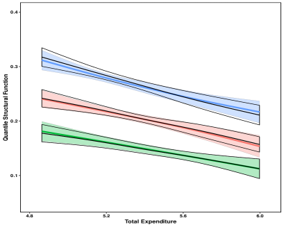
(a) $M=2$.

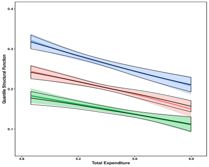
(b) $M=3$.

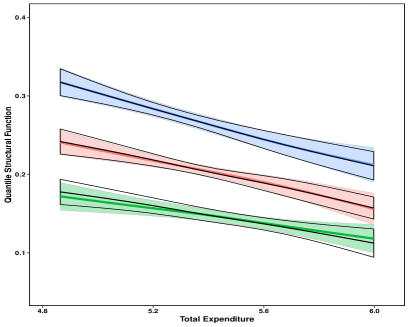
(c) $M=5$.

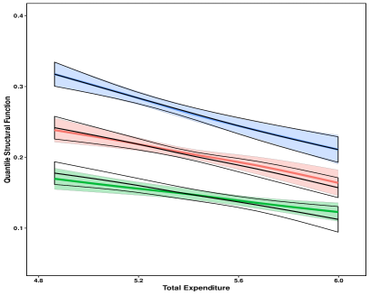
(d) $M=15$.

Figure 5.1: Design 1. QSF for food with discrete instrument $\widetilde{Z}$ (coloured) and with continuous instrument $Z^{*}$ (black).

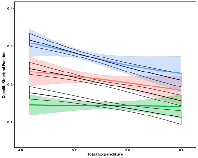
(a) $M=2$.

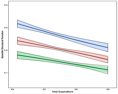
(b) $M=3$.

(c) $M=5$.

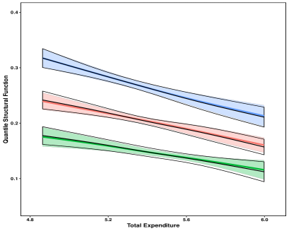
(d) $M=15$.

Figure 5.2: Design 2. QSF for food with discrete instrument $\widetilde{Z}$ (coloured) and with continuous instrument $Z^{*}$ (black).

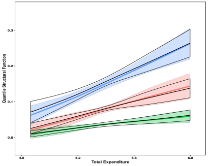
(a) $M=2$.

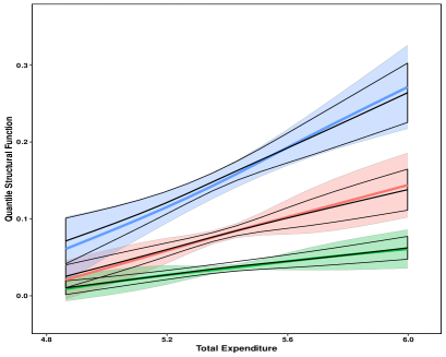
(b) $M=3$.

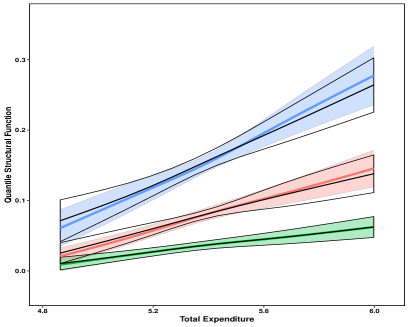
(c) $M=5$.

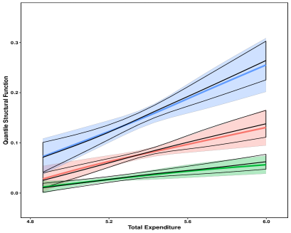
(d) $M=15$.

Figure 5.3: Design 1. QSF for leisure with discrete instrument $\widetilde{Z}$ (coloured) and with continuous instrument $Z^{*}$ (black).

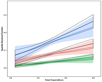
(a) $M=2$.

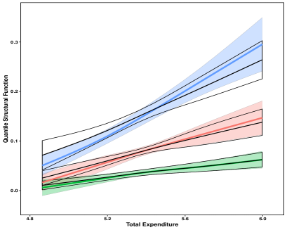
(b) $M=3$.

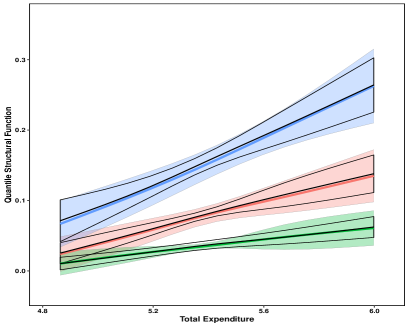
(c) $M=5$.

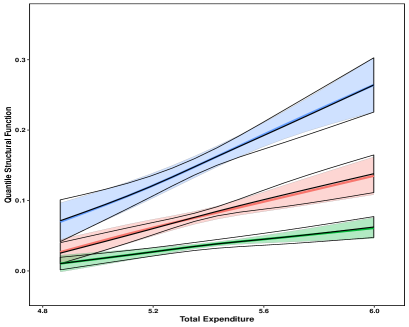
(d) $M=15$.

Figure 5.4: Design 2. QSF for leisure with discrete instrument $\widetilde{Z}$ (coloured) and with continuous instrument $Z^{*}$ (black).

Figures 5.1 and 5.2 show the $0.25$, $0.5$ and $0.75$-QSFs for food estimated with each set of four instruments, respectively, as well as the corresponding benchmark QSFs estimated using the original continuous instrument $Z^{*}$. Figures 5.3 and 5.4 show the corresponding QSFs for leisure. For comparison purposes the implementation is exactly as in Chernozhukov et al. (2017). We report weighted bootstrap 90%-confidence bands that are uniform over the support regions of the displayed QSFs, constructed with $250$ bootstrap replications. Our empirical results show that both discretisation schemes deliver very similar QSF estimates and confidence bands that capture the main features of the benchmark QSFs estimated with a continuous instrument. The largest deviations from the benchmark QSFs occur for $M=2$ and the non uniform Design 2, where the first value of $\widetilde{Z}$ is allocated to $6\%$ of the observations only.

For this dataset the main features of Engel curves for food and leisure are well captured when estimation is performed with a discrete valued instrumental variable. Overall our empirical findings support our identification results and illustrate the use of discrete instruments for the estimation of structural functions in triangular systems.

Appendix A Proof of Main Results

A.1 Proof of Theorem 1

Proof.

Part (i). The proof builds on the proof of Lemma S3 in Spady and Stouli (2018). The matrix $E\left[w(X,V)w(X,V)^{\prime}\right]$ is of the form

$$E\left[w(X,V)w(X,V)^{\prime}\right] =E\left[\{p(X)\otimes q(V)\}\{p(X)\otimes q(V)\}^{\prime}\right]$$

$$=E\left[\{p(X)p(X)^{\prime}\}\otimes\{q(V)q(V)^{\prime}\}\right]$$

$$=E\left[\begin{array}[]{cc}p(X)p(X)^{\prime}&p(X)p(X)^{\prime}V\\ p(X)p(X)^{\prime}V&p(X)p(X)^{\prime}V^{2}\end{array}\right].$$

Assumption 2(a) implies that $E[p(X)p(X)^{\prime}]$ is positive definite. Thus $E\left[w(X,V)w(X,V)^{\prime}\right]$ is positive definite if and only if the Schur complement of $E[p(X)p(X)^{\prime}]$ in $E\left[w(X,V)w(X,V)^{\prime}\right]$ is positive definite (Boyd and Vandenberghe, 2004, Appendix A.5), i.e., if and only if

$$\varUpsilon:=E\left[p(X)p(X)^{\prime}V^{2}\right]-E\left[p(X)p(X)^{\prime}V\right]E\left[p(X)p(X)^{\prime}\right]^{-1}E\left[p(X)p(X)^{\prime}V\right]$$

satisfies $\textrm{det}(\varUpsilon)>0$.

With

$$\Xi=E\left[p(X)p(X)^{\prime}V\right]E\left[p(X)p(X)^{\prime}\right]^{-1},$$

we have that

$$\varUpsilon=E\left[\left\{p(X)V-\Xi p(X)\right\}\left\{p(X)V-\Xi p(X)\right\}^{\prime}\right],$$

a finite positive definite matrix, if and only if for all $\lambda\neq 0$ there is no $d$ such that $\Pr[\{\lambda^{\prime}p(X)\}V=d^{\prime}\{\Xi p(X)\}]>0$; this is an application of the Cauchy-Schwarz inequality for matrices stated in Tripathi (1999).

For $\widetilde{\mathcal{X}}\subseteq\mathcal{X}_{V}^{o}$, positive definiteness of $E[1(X\in\widetilde{\mathcal{X}})p(X)p(X)^{\prime}]$ under Assumption 2(a) implies that for all $\lambda\neq 0$, $E[1(X\in\widetilde{\mathcal{X}})\{\lambda^{\prime}p(X)\}^{2}]>0$, which implies that for all $\lambda\neq 0$, the set $\{x\in\widetilde{\mathcal{X}}\,:\,\lambda^{\prime}p(x)\neq 0\}$ has positive probability. By definition of $\mathcal{V}_{x}$ and the variance, we have that $\textrm{Var}(V\mid X=x)>0$ for each $x\in\mathcal{X}_{V}^{o}$. Thus for all $\lambda\neq 0$, by $\Xi$ being a constant matrix, there is no $d$ such that $\Pr[\{\lambda^{\prime}p(X)\}V=d^{\prime}\{\Xi p(X)\}]>0$, and $E\left[w(X,V)w(X,V)^{\prime}\right]$ is positive definite.

Part (ii). The proof is similar to Part (i). ∎

A.2 Proof of Theorem 2

Proof.

By iterated expectations, $E\left[w(X,V)w(X,V)^{\prime}\right]$ can be expressed as

$$E\left[w(X,V)w(X,V)^{\prime}\right]=E\left[\{p(X)p(X)^{\prime}\}\otimes E[q(V)q(V)^{\prime}\mid X]\right].$$

We show that $E\left[w(X,V)w(X,V)^{\prime}\right]$ is positive definite. By Assumption 2(a), there is a positive constant $B$ such that

$$E\left[\{p(X)p(X)^{\prime}\}\otimes E[q(V)q(V)^{\prime}\mid X]\right] \geq E\left[1(X\in\widetilde{\mathcal{X}})\{p(X)p(X)^{\prime}\}\otimes\lambda_{\min}(X)I_{K}\right]$$

$$\geq E\left[1(X\in\widetilde{\mathcal{X}})\{p(X)p(X)^{\prime}\}\right]\otimes BI_{K},$$

where $I_{K}$ is the $K\times K$ identity matrix, and the inequality means no less than in the usual partial ordering for positive semi-definite matrices. The conclusion then follows by the matrix following the last inequality being positive definite by Assumption 2(a).

Under Assumption 2(b) the proof is similar upon using that $E\left[w(X,V)w(X,V)^{\prime}\right]=E\left[E[p(X)p(X)^{\prime}\mid V]\otimes\{q(V)q(V)^{\prime}\}\right]$. ∎

A.3 Proof of Theorem 3

Proof.

By Theorem 2 the matrix $E\left[w(X,V)w(X,V)^{\prime}\right]$ exists and is positive definite. The result then follows by Theorem 1 in Chernozhukov et al. (2017). ∎

A.4 Proof of Theorem 4

Proof.

The result follows from the proof of Theorem 1 in Newey and Stouli (2018). ∎

A.5 Proof of Theorem 5

Proof.

Under Assumption 3(a), $q_{\tau}\left(V\right)$ is identified for each $\tau\in\mathcal{T}$ by Theorem 4. This implies that, for $\mathcal{T}=\mathcal{Y}$, the conditional CDF $F_{Y\mid XV}(y\mid X,V)=\Gamma(p(X)^{\prime}q_{y}(V))$ is unique with probability one for each $y\in\mathcal{Y}$, since $p\left(X\right)$ and $\Gamma$ are known functions. The structural functions are then identified by (2.2) in the main text. For $\mathcal{T}=\mathcal{U}$, when $Y$ is continuous the conditional quantile function $Q_{Y\mid XV}(u\mid X,V)=p(X)^{\prime}q_{u}(V)$ is unique with probability one for each $u\in\mathcal{U}$. Since $y\mapsto F_{Y\mid XV}(y\mid XV)$ is the inverse function of $u\mapsto Q_{Y\mid XV}(u\mid X,V)$, the structural functions are also identified by (2.2) in the main text. ∎

Appendix B Formal Statement of Remark 2

Proposition 1.

(i) Let $q(V)=(1,V)^{\prime}$. If Assumption 2(a) holds with $\widetilde{\mathcal{X}}\subseteq\mathcal{X}_{V}^{o}$ then it also holds with $\widetilde{\mathcal{X}}\subseteq\mathcal{X}_{V}^{*}$. (ii) Let $p(X)=(1,X)^{\prime}$. If Assumption 2(b) holds with $\widetilde{\mathcal{V}}\subseteq\mathcal{V}_{X}^{o}$ then it also holds with $\widetilde{\mathcal{V}}\subseteq\mathcal{V}_{X}^{*}$.

Proof.

Each $x\in\mathcal{X}_{V}^{o}$ satisfies $|\mathcal{V}_{x}|\geq 2$, which by the definitions of $\mathcal{V}_{x}$ and the variance implies that $\textrm{Var}(V\mid X=x)\geq B>0$. For $q(V)=(1,V)^{\prime}$, the smallest eigenvalue of $E[q(V)q(V)^{\prime}\mid X=x]$ is then bounded away from zero for each $x\in\mathcal{X}_{V}^{o}$, by Lemma 1 below. Therefore each $x\in\mathcal{X}_{V}^{o}$ also satisfies $x\in\mathcal{X}_{V}^{*}$, so that $\mathcal{X}_{V}^{o}\subseteq\mathcal{X}_{V}^{*}$. The result for Part (i) follows, and the proof for Part (ii) is similar. ∎

Lemma 1.

For a set of random variables $\{X(t)\}_{t\in\overline{\mathcal{T}}}$ such that $E[X(t)^{2}]\leq C$ and $\text{Var}(X(t))\geq B>0$, the smallest eigenvalue of

$$\Sigma(t)=E\left[\left(\begin{array}[]{c}1\\ X(t)\end{array}\right)\left(\begin{array}[]{cc}1&X(t)\end{array}\right)\right]$$

is bounded away from zero.

Proof.

We have $\textrm{det}(\Sigma(t))=\textrm{Var}(X(t))=\lambda_{\max}(t)\lambda_{\min}(t)$, where $\lambda_{\max}(t)$ and $\lambda_{\min}(t)$ are the largest and smallest eigenvalues of $\Sigma(t)$, respectively. Note that, for some positive constant $\widetilde{C}<\infty$ and all $t\in\overline{\mathcal{T}}$,

$$\lambda_{\max}(t)=\sup_{\lambda:||\lambda||=1}\lambda^{\prime}\Sigma(t)\lambda\leq||\lambda||^{2}||\Sigma(t)||\leq||\Sigma(t)||\leq\widetilde{C}$$

by $E[X(t)^{2}]$ bounded. Therefore

$$\lambda_{\min}(t)=\frac{\textrm{Var}(X(t))}{\lambda_{\max}(t)}\geq\frac{\textrm{Var}(X(t))}{\widetilde{C}}\geq\frac{B}{\widetilde{C}},$$

and the result follows. ∎

Appendix C Estimation of Structural Functions

Here we give a summary of the key steps in the implementation of the quantile regression-based estimators for structural functions proposed by Chernozhukov et al. (2017). A detailed description and implementation algorithms for estimation and the weighted bootstrap procedures are given in Chernozhukov et al. (2017).

The estimators implemented in the empirical application have three main stages. In the first stage, we estimate the control variable, $\{\widehat{V}_{i}\}_{i=1}^{n}$. In the second stage, we estimate the distribution CRF, $\widehat{F}_{Y\mid XZ_{1}V}(y\mid x,z_{1},v)$. In the third and final stage, estimators $\widehat{G}(y,x)$, $\widehat{Q}(\tau,x)$ and $\widehat{\mu}(x)$ of the distribution, quantile and average structural functions, respectively, are obtained.

First stage. [Control function estimation] Denoting the usual check function by $\rho_{v}(z)=(v-1(z<0))z$, the quantile regression estimator of $F_{X\mid Z}$ is, for $(x,z)\in\mathcal{X}\mathcal{Z}$,

$$\widehat{F}_{X\mid Z}(x\mid z) = \epsilon+\int_{\epsilon}^{1-\epsilon}1\left\{\widehat{\pi}(v)^{\prime}[s(\widetilde{z})\otimes r(z_{1})]\leq x\right\}dv,$$ (C.1)

$$\widehat{\pi}(v) \in \arg\min_{\pi\in\mathbb{R}^{\text{dim}(Z)}}\sum_{i=1}^{n}\rho_{v}(X_{i}-\pi^{\prime}[s(\widetilde{Z}_{i})\otimes r(Z_{1i})]),$$ (C.2)

for some small constant $\epsilon>0$. The adjustment in the limits of the integral in (C.1) avoids tail estimation of quantiles. In practice, for $\epsilon$ in $(0,0.5)$ (e.g., $\epsilon=0.01$) and a fine mesh of $T$ values $\{\epsilon=v_{1}<\cdots<v_{T}=1-\epsilon\}$, estimate $\{\widehat{\pi}(v_{t})\}_{t=1}^{T}$ by solving (C.2). Obtain the control function estimator $\widehat{F}_{X\mid Z}(X_{i}\mid Z_{i})$ as in (C.1), and set $\widehat{V}_{i}=\widehat{F}_{X\mid Z}(X_{i}\mid Z_{i})$, for $i\in\{1,\ldots,n\}$.

Second stage. [Distribution CRF estimation] The quantile regression estimator of $F_{Y\mid XZ_{1}V}$ is, for $(y,x,z_{1},v)\in\mathcal{Y}\mathcal{X}\mathcal{Z}_{1}\mathcal{V}$,

$$\widehat{F}_{Y\mid XZ_{1}V}(y\mid x,z_{1},v) = \epsilon+\int_{\epsilon}^{1-\epsilon}1\left\{\widehat{\beta}(u)^{\prime}w(x,z_{1},v)\leq y\right\}du,$$ (C.3)

$$\widehat{\beta}(u) \in \arg\min_{\beta\in\mathbb{R}^{\text{dim}(w(X,Z_{1},V))}}\sum_{i=1}^{n}\rho_{u}(Y_{i}-\beta^{\prime}w(X_{i},Z_{1i},\widehat{V}_{i})),$$ (C.4)

In practice, for $\epsilon$ in $(0,0.5)$ (e.g., $\epsilon=0.01$) and a fine mesh of $T$ values $\{\epsilon=u_{1},\ldots,u_{T}=1-\epsilon\}$, estimate $\{\widehat{\beta}(u_{t})\}_{t=1}^{T}$ by solving (C.4). Obtain the distribution CRF estimator $\widehat{F}_{Y\mid XZ_{1}V}(y\mid x,Z_{1i},\widehat{V}_{i})$ as in (C.3).

Third stage. [Structural functions estimation] Let $\mathcal{Y}^{+}=\mathcal{Y}\cap[0,\infty)$ and $\mathcal{Y}^{-}=\mathcal{Y}\cap(-\infty,0)$. Given estimates $(\{\widehat{V}_{i}\}_{i=1}^{n},\widehat{F}_{Y\mid XZ_{1}V})$, the estimator for the distribution structural function takes the form

$$\widehat{G}(y,x)=\frac{1}{n}\sum_{i=1}^{n}\widehat{F}_{Y\mid XZ_{1}V}(y\mid x,Z_{1i},\widehat{V}_{i}).$$

Given the distribution structural function estimate, the QSF estimator is defined as

$$\widehat{Q}(p,x)=\int_{\mathcal{Y}^{+}}1\{\widehat{G}(y,x)\leq p\}dy-\int_{\mathcal{Y}^{-}}1\{\widehat{G}(y,x)\geq p\}dy,$$ (C.5)

and the average structural function estimator as

$$\widehat{\mu}(x)=\int_{\mathcal{Y}^{+}}[1-\widehat{G}(y,x)]\nu(dy)-\int_{\mathcal{Y}^{-}}\widehat{G}(y,x)\nu(dy),$$ (C.6)

where $\nu$ is either the counting measure when $\mathcal{Y}$ is countable or the Lebesgue measure otherwise. When the set $\mathcal{Y}$ is uncountable and bounded, we approximate the previous integrals by sums over a fine mesh of equidistant points $\mathcal{Y}_{S}:=\{\inf[y\in\mathcal{Y}]=y_{1}<\cdots<y_{S}=\sup[y\in\mathcal{Y}]\}$ with mesh width $\delta$ such that $\delta\sqrt{n}\to 0$. For example, (C.5) and (C.6) are approximated by

$$\widehat{G}(y,x)=\frac{1}{n}\sum_{i=1}^{n}\widehat{F}_{Y\mid XZ_{1}V}(y\mid x,Z_{1i},\widehat{V}_{i}),$$

$$\widehat{Q}_{S}(p,x)=\delta\sum_{s=1}^{S}\left[1(y_{s}\geq 0)-1\{\widehat{G}(y_{s},x)\geq p\}\right],\,\widehat{\mu}_{S}(x)=\delta\sum_{s=1}^{S}\left[1(y_{s}\geq 0)-\widehat{G}(y_{s},x)\right].$$

The choices of $\epsilon$ and $T$ can differ across stages. In the empirical application we set $\epsilon=0.01$ and $T=599$ throughout. For the third stage, we approximate the integrals in (C.5)-(C.6) using $S=599$ points. Overall, for this application the estimates are not very sensitive to $T$, and are also robust to varying values of $\epsilon$ and $S$.

References

- [1] Belloni, A., and V. Chernozhukov, 2011, 1-penalized quantile regression in high-dimensional sparse models. Annals of Statistics 39, pp. 82-130.
- [2] Belloni, A., and V. Chernozhukov, 2011, Fernandez-Val, I., and C. Hansen, 2017, Program evaluation and causal inference with high-dimensional data. Econometrica 85, pp. 233-298.
- Boyd & Vandenberghe [2004] Boyd, S. P. and L. Vandenberghe, 2004, Convex optimization. Cambridge University Press, Cambridge.
- [4] Blundell, R., and J. L. Powell, 2003, Endogeneity in nonparametric and semiparametric regression models. Econometric society monographs 36, pp. 312-357.
- [5] Blundell, R., and J. L. Powell, 2004, Endogeneity in semiparametric binary response models. The Review of Economic Studies 71, pp. 655-679.
- [6] Blundell, R., Chen, X., and D. Kristensen, 2007, Semi-nonparametric IV estimation of shape-invariant Engel curves. Econometrica 75, pp. 1613-1669.
- [7] Chernozhukov, V., Fernandez-Val, I., and A. Kowalski, 2015, Quantile regression with censoring and endogeneity. Journal of Econometrics 186, pp. 201-221.
- [8] Chernozhukov, V., Fernandez-Val, I., and B. Melly, 2013, Inference on counterfactual distributions. Econometrica 81, 2205-2268.
- [9] Chernozhukov, V., Fernandez-Val, I. Newey, W., Stouli, S. and F. Vella, 2017, Semiparametric estimation of structural functions in nonseparable triangular models. eprint arXiv:1711.02184.
- [10] D’Haultfœuille, X. and P. Février, 2015, Identification of nonseparable triangular models with discrete instruments. Econometrica 83, pp. 1199-1210.
- [11] Fernandez-Val, I. Van Vuuren, A. and F. Vella, 2017, Nonseparable sample selection models with censored selection rules. eprint arXiv:1801.08961.
- [12] Florens, J. P., Heckman, J. J., Meghir, C. and E. Vytlacil, 2008, Identification of treatment effects using control functions in models with continuous, endogenous treatment and heterogeneous effects. Econometrica 76, pp. 1191-1206.
- [13] Hausman, J. A. and W. K. Newey, 2016, Individual heterogeneity and average welfare. Econometrica 84, pp.1225-1248.
- [14] Hausman, J. A. and D. Wise, 1978, A conditional probit model for qualitative choice: discrete decisions recognizing interdependence and heterogeneous preferences. Econometrica 46, pp. 403-426.
- Imbens [2000] Imbens, G. W., 2000, The role of the propensity score in estimating dose-response functions. Biometrika 87(3), pp. 706-710.
- [16] Imbens, G. and W. K. Newey, 2009, Identification and estimation of triangular simultaneous equations models without additivity. Econometrica 77, pp. 1481-1512.
- Kitamura and Stoye [2018] Kitamura, Y. and J. Stoye, 2018, Nonparametric analysis of random utility models. Econometrica 86, pp.1883-1909.
- Masten and Torgovitsky [2016] Masten, M. and A. Torgovitsky, 2016, Identification of instrumental variable correlated random coefficients models. Review of Economics and Statistics 98, pp. 1001–1005.
- [19] McFadden, D., 1973, Conditional logit analysis of qualitative choice behavior, in: P. Zarambka (Ed.), Frontiers in econometrics. New York: Academic Press.
- [20] Newey, W.K. and D. McFadden, 1994, Large sample estimation and hypothesis testing, in: Engle, R. and D. McFadden (Eds.), Handbook of econometrics. Elsevier, Berlin, pp. 2111-2245.
- [21] Newey, W. K. and S. Stouli, 2018, Heterogenous coefficients, discrete instruments, and identification of treatment effects. eprint arXiv:1811.09837.
- [22] Rosenbaum, P. R. and D. B. Rubin, 1983, The central role of the propensity score in observational studies for causal effects. Biometrika 70, pp.41-55.
- [23] Spady, R. H. and S. Stouli, 2018, Dual regression. Biometrika 105, pp. 1-18.
- [24] Tibshirani, R., 1996, Regression shrinkage and selection via the Lasso. Journal of the Royal Statistical Society: Series B 58, 267-288.
- [25] Torgovitsky, A., 2015, Identification of nonseparable models using instruments with small support. Econometrica 83, pp. 1185-1197.
- Wooldridge [2004] Tripathi, G., 1999, A matrix extension of the Cauchy-Schwarz inequality. Economics Letters 63, pp. 1-3.
- [27] Wooldridge, J. M., 2004, Estimating average partial effects under conditional moment independence assumptions. Cemmap working paper CWP03/04.