We derive a graph expansion for the thermal partition function of solvable two-dimensional models with boundaries. This expansion of the integration measure over the virtual particles winding around the time cycle is obtained with the help of the matrix-tree theorem. The free energy is a sum over all connected graphs, which can be either trees or trees with one loop. The generating function for the connected trees satisfies a non-linear integral equation, which is equivalent to the TBA equation. The sum over connected graphs gives the bulk free energy as well as the exact $g$-functions for the two boundaries. We reproduced the integral formula conjectured by Dorey, Fioravanti, Rim and Tateo, and proved subsequently by Pozsgay. Our method can be extended to the case of non-diagonal bulk scattering and diagonal reflection matrices with proper regularization.

1 Introduction

The notion of integrability has been extended to systems with boundary by Ghoshal and Zamolodchikov [1]. With the Yang-Baxter equation, unitarity, analyticity and crossing symmetry for both bulk scattering matrix and boundary reflection matrix, a model with integrable boundary is expected to be exactly solved. One of the simplest observables in such system is its free energy in large volume limit and at finite temperature. Unlike in periodic systems, this free energy contains a volume-independent correction, also known as the boundary entropy or $g$-function [2].

The first attempt to compute $g$-function was carried out by LeClair, Mussardo, Saleur and Skorik [3], using the Thermodynamics Bethe Ansatz (TBA) saddle point approximation. They obtained an expression similar to the bulk TBA free energy

$$\log(g_{a}g_{b})^{\textnormal{saddle}}(R)=\frac{1}{2}\int_{-\infty}^{+\infty}\frac{du}{2\pi}\,\Theta_{ab}(u)\log[1+e^{-\epsilon(u)}],$$ (1.1)

where $u$ is the rapidity variable, $\epsilon$ is the pseudo-energy at inverse temperature $R$ and $\Theta$ term involves the bulk scattering and the boundary reflection matrices.

It was later shown by Woynarovich [4] that another volume-independent contribution is produced by the fluctuation around the TBA saddle point. The result can be written as a Fredholm determinant

$$\log(g_{a}g_{b})^{\textnormal{fluc}}(R)=-\log\det(1-\hat{K}^{+}),$$ (1.2)

where the kernel $\hat{K}^{+}$ involves the pseudo-energy and the bulk scattering matrix but not the reflection matrices. In other words, this fluctuation around the saddle point is boundary independent. A major problem of Woynarovich’s computation is that it also predicts a similar term for periodic systems, while it is known that there is no such correction.

Dorey, Fioravanti, Rim and Tateo [5] took a different approach towards this problem. They started with the definition of the partition function as a thermal sum over a complete set of states labelled by mode numbers. In the infinite volume limit, this sum can be replaced by integrals over rapidity. The integrands were explicitly worked out for small number of particles. Based on these first terms and the structure of TBA saddle point result (1.1), the authors advanced a conjecture about the boundary-independent part of $g$-function. Their proposal has the structure of a Leclair-Mussardo type series

$$\log(g_{a}g_{b})(R) =\log(g_{a}g_{b})^{\textnormal{saddle}}(R)$$

$$+\sum_{n\geq 1}\frac{1}{n}\prod_{j=1}^{n}\int_{-\infty}^{+\infty}\frac{du_{j}}{2\pi}\frac{1}{1+e^{\epsilon(u_{j})}}K(u_{1}+u_{2})K(u_{2}-u_{3})...K(u_{n}-u_{1}),$$ (1.3)

where $K$ is the logarithmic derivative of the bulk scattering matrix.

Pozsgay [6] (see also Woynarovich [7]) argued that the same expression for $g$-function could be obtained from a refined version of TBA saddle point approximation. He noticed that the mismatch between (1.2) and the series in (1.3) is resolved if one uses a non-flat measure for the TBA functional integration. This non-trivial measure comes from the Jacobian of the change of variables from mode number to rapidity, and represents the continuum limit of the Gaudin determinant.

The fluctuation around the saddle point involves only diagonal elements of this Gaudin matrix, resulting in the inverse power of the Fredholm determinant $\det(1-\hat{K}^{+})$. On the other hand, the functional integration measure contains the off-diagonal elements as well, which constitute another Fredholm determinant $\det(1-\hat{K}^{-})$. Pozsgay rewrote the result (1.3) in terms of these two Fredholm determinants

$$\log(g_{a}g_{b})(R)=\log(g_{a}g_{b})^{\textnormal{saddle}}(R)+\log\det\frac{1-\hat{K}^{-}}{1-\hat{K}^{+}}.$$ (1.4)

The two kernels $\hat{K}^{\pm}$ can be read off from the asymptotic Bethe equations. For a periodic system, they happen to be the same and the effects from the fluctuation and the measure cancel each other.

It is important to distinguish the Jacobians in [5] from the one in [6]. The former appear in each term of the cluster expansion while the latter is obtained from the thermodynamics state that minimizes the TBA functional action. Put it simply, the Jacobian in [6] is the thermal average of all the Jacobians in [5].

In this paper, we derive this known result for $g$-function, following the strategy of [5]: writing the partition function as a sum over mode numbers and replacing it by an integral over phase space in the infinite volume limit. In contrast to [5], we are able to exactly carry out the cluster expansion, by virtue of the matrix-tree theorem [8]. This theorem allows us to write the Jacobian for a finite number of particles as a sum over diagrams. Consequently, the $g$-function is expressed as a sum over graphs with no loops (trees) and graphs with one loop. These combinatorial objects possess simple structure and their sum can be written in the form (1.3) or (1.4). Compared to [6], the Gaussian fluctuations and the measure can be respectively interpreted as the sum over two types of loops. Our final result coincides with the one of [6], but our method allows an exact treatment of each term in the canonical partition sum, before the thermodynamical limit. Such advantage makes it potentially useful in the computation of more subtle objects such as correlation functions. This method has been applied for the free energy and one point function of a local observable of a periodic system [9],[10],[11]. The same idea has been used to derive the equation of state in Generalized Hydrodynamics [12].

Generalization to a theory with $n$ species of particles interacting via diagonal bulk scattering and diagonal reflection matrices is straightforward. The graphs now involve $n$ types of vertices and the Fredholm kernels are $n\times n$ matrices. We also comment on how the g-function of a theory solved by Nested Bethe Ansatz can be obtained through a regularization procedure. We implement such procedure for a concrete example in another work [13].

The paper is structured as follows. In section 2 we recall the definition of $g$-function and spell out the Fredholm determinant formula (1.4) for a massive theory with diagonal bulk and boundary scattering. In section 3 we develop the combinatorics needed to sum up the cluster expansion and express the partition function on a cylinder as a sum over (multi)wrapping virtual particles. In section 4 we expand, with help of the matrix-tree theorem, the canonical partition function on a cylinder as a sum over certain set of Feynman graphs. In section 5 we perform the sum and recover the expression for the $g$-function. We compute the excited state g-function at the end of the section. In section 6 we generalise our method to theories of more than one type of particle with diagonal scatterings. We also establish a protocol to deal with g-function of theories solved by Nested Bethe Ansatz. The two appendices present two different proofs of the matrix-tree theorem in the form used in this paper.

2 Bulk and boundary free energy of a massive integrable field theory

The $g$-function, also known as boundary entropy or ground-state degeneracy, was first introduced by Affleck and Ludwig [2] and since then has been given many physical interpretations. In this paper we shall look at this multifaceted object as the non-extensive contribution to free energy of a system with boundaries.

Let us consider an $1+1$ dimensional field theory with a single massive excitation above the vacuum, defined in an open interval of length $L$, whose boundaries will be denoted by $a$ and $b$ . The momentum and energy of a particle are parameterized by its rapidity $p=p(u),E=E(u)$. The theory is integrable with a two-to-two bulk scattering phase $S(u,v)$ and reflection factors $R_{a}(u),R_{b}(u)$ at the boundaries. They satisfy a set of conditions [1], among which the unitarity condition

$$S(u,v)S(v,u)=R_{a}(u)R_{a}(-u)=R_{b}(u)R_{b}(-u)=1.$$ (2.1)

The bulk scattering phase does not necessarily depend on the difference between rapidities. We assume a milder condition

$$S(u,-v)S(-u,v)=1,$$ (2.2)

as well as $S(u,u)=-1$.

The partition function at inverse temperature $R$ is defined by the thermal trace

$$Z_{ab}(R,L)={\rm Tr}\;e^{-H_{ab}(L)R},$$ (2.3)

where $H_{ab}(L)$ is the Hamiltonian of the theory living on a segment of length $L$ with boundary conditions $a$ and $b$. One can consider in parallel the partition function of a theory defined on a circle of length $L$

$$Z(R,L)={\rm Tr}\;e^{-H(L)R}.$$ (2.4)

The boundary entropy of the open system is given by the difference in the two free energies

$$\mathcal{F}_{ab}(R,L)\equiv\log Z_{ab}(R,L)-\log Z(R,L).$$ (2.5)

The $g$-function is defined as the contribution of a single boundary to the free energy. To compute it, we pull the two boundaries far away from each other to avoid interference

$$\log g_{a}(R)=\frac{1}{2}\lim_{L\to\infty}\mathcal{F}_{aa}(R,L).$$ (2.6)

Compared to the usual definition of $g$-function given in perturbed CFTs literature, our definition seems to be over-simplifying. This is due to our specific choice of normalization of partition functions. More precisely, we have fixed the ground state energy in the $L\to\infty$ limit of both Hamiltonians $H({L})$ and $H_{ab}(L)$ to zero by discarding the bulk energy density as well as its non-extensive boundary contributions.

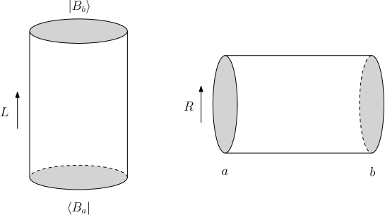
Figure 1: Two equivalent ways of evaluating the partition function on a cylinder.

In a relativistic theory there is a mirror transformation exchanging the roles of space and time

$$\tilde{p}(u)=-iE(u^{\gamma}),\ \ \ \tilde{E}(u)=-ip(u^{\gamma}),$$ (2.7)

where $u^{\gamma}$ means analytical continuation in the rapidity variable which assures that the mirror particle has positive energy $\tilde{E}$ and real momentum $\tilde{p}$. The inverse is true only if the mirror theory coincides with the original one. In this case the natural parametrisation is $p=m\sinh u,E=m\cosh u$ and $u^{\gamma}=u+i\pi/2$. The product of two mirror transformations, $u\to u+i\pi$, gives a crossing transformation.

In terms of the mirror theory, defined on a circle with circumference $R$, the partition function with periodic boundary conditions (2.4) takes a similar form

$$Z(R,L)={\rm Tr}\;e^{-\tilde{H}(R)L},$$ (2.8)

where the trace is in the Hilbert space of the mirror theory. In contrast, after a mirror transformation the thermal partition function with open boundary conditions becomes the overlap of an initial state $\langle B_{a}|$ and a final state $|B_{b}\rangle$ defined on a circle of circumference $R$ after evolution at mirror time $L$ [1]. Evaluated in the mirror theory, the partition function (2.3) reads

$$Z_{ab}(R,L)=\langle B_{a}|e^{-\tilde{H}(R)L}|B_{b}\rangle.$$ (2.9)

Although the partition function is the same, the physics is rather different in the two channels. In the mirror theory, the $g$-function provides information about overlapping of the boundary states and the ground state at finite volume. To see this, we write (2.9) as a sum over eigenstates $|\psi\rangle$ of the periodic Hamiltonian $\tilde{H}(R)$

$$\langle B_{a}|e^{-\tilde{H}(R)L}|B_{b}\rangle=\sum_{|\psi\rangle}\frac{\langle B_{a}|\psi\rangle}{\sqrt{\langle\psi|\psi\rangle}}e^{-L\tilde{E}(|\psi\rangle)}\frac{\langle\psi|B_{b}\rangle}{\sqrt{\langle\psi|\psi\rangle}}.$$

In the large $L$ limit, this sum is dominated by a single term corresponding to the ground state $|\psi_{0}\rangle$. The $g$-function is then given by the overlap between this state and the boundary state

$$g_{a}(R)=\frac{\langle B_{a}|\psi_{0}\rangle}{\sqrt{\langle\psi_{0}|\psi_{0}\rangle}}.$$ (2.10)

An expression for $g$-function was conjectured in [5] and proven in [6]. Here we write down this result for the case where the bulk scattering matrix is not of difference form. Let us denote respectively by $K,K_{a}$ and $K_{b}$ the logarithmic derivatives of the bulk scattering phase and the boundary reflection factors associated with the boundaries $a$ and $b$

$$K(u,v)=-i\partial_{u}\log S(u,v),\quad K_{a}(u)=-i\partial_{u}\log R_{a}(u),\quad K_{b}(u)=-i\partial_{u}\log R_{b}(u).$$

It follows from (2.1) and (2.2) that

$$K_{a}(u)=K_{a}(-u),\quad K_{b}(u)=K_{b}(-u),\quad K(u,-v)=K(-u,v).$$ (2.11)

Let us also define

$$\Theta_{\star}(u)\equiv K_{\star}(u)-K(u,-u)-\pi\delta(u),\quad\star=a,b.$$ (2.12)

Then the expression for $g$-function found in [6] reads

$$\log g_{a}(R)=\frac{1}{2}\int_{-\infty}^{+\infty}\frac{du}{2\pi}\,\Theta_{a}(u)\log(1+e^{-\epsilon(u)})+\frac{1}{2}\log\det\frac{1-\hat{K}^{-}}{1-\hat{K}^{+}},$$ (2.13)

where $\epsilon$ is the pseudo-energy at inverse temperature $R$

$$e^{-\epsilon(u)}=e^{-E(u)R}\exp\bigg{[}\int_{-\infty}^{\infty}\frac{dv}{2\pi}K(v,u)\log(1+e^{-\epsilon(v)})\bigg{]}.$$ (2.14)

The kernels $\hat{K}^{\pm}$ have support on the positive real axis and their action is given by

$$\hat{K}^{\pm}F(u)=\int_{0}^{\infty}\frac{dv}{2\pi}\big{[}K(u,v)\pm K(u,-v)\big{]}\frac{1}{1+e^{\epsilon(v)}}F(v).$$ (2.15)

In the next sections we will derive the expression (2.13) by evaluating the partition function in the $R$-channel, namely equation (2.3), in the limit when $L$ is large. In order to do that, we will insert a decomposition of the identity in a complete basis of eigenstates of the Hamiltonian $H_{ab}(L)$ and perform the thermal trace.

3 Partition function on a cylinder as a sum over wrapping particles

3.1 Asymptotic Bethe equations in presence of boundaries

The $g$-function (2.6) is extracted by taking the limit of large volume $L$. In this limit, we can diagonalize the Hamiltonian $H_{ab}(L)$ using the technique of Bethe ansatz.

Consider an $N$-particle eigenstate $|\textbf{u}\rangle=|u_{1},u_{2},...,u_{N}\rangle$. To obtain the Bethe Ansatz equations in presence of two boundaries, we follow a particle of rapidity $u_{j}$ as it propagates to a boundary and is reflected to the opposite direction. It continues to the other boundary, being reflected for a second time and finally comes back to its initial position, finishing a trajectory of length $2L$. During its propagation, it scatters with the rest of the particles twice, once from the left and once from the right. This process translates into the quantisation condition of the state $|\textbf{u}\rangle$

$$e^{2ip(u_{j})L}R_{a}(u_{j})R_{b}(u_{j})\prod_{k\neq j}^{N}S(u_{j},u_{k})S(u_{j},-u_{k})=1,\quad\forall j=1,...,N.$$ (3.1)

We can write these equations in logarithmic form by introducing a new set of variables: the total scattering phases $\phi_{1},\phi_{2},...,\phi_{n}$ defined by

$$\phi_{j}(\textbf{u})\equiv 2p(u_{j})L-i\log[R_{a}R_{b}(u_{j})\prod_{k\neq j}^{N}S(u_{j},u_{k})S(u_{j},-u_{k})],\quad\forall j=1,...,N.$$ (3.2)

In terms of these variables, the quantization of state $|\textbf{u}\rangle$ reads

$$\phi_{j}(\textbf{u})=2\pi n_{j}\quad\forall j=1,...,N\quad\textnormal{with }n_{j}\in\mathbb{Z}.$$ (3.3)

The next step is to impose particle statistics and indistinguishability. In periodic systems, simply taking the mode numbers $n_{j}$ to be all different automatically satisfies both principles. However in the presence of boundary two particles having the same mode numbers but of opposite signs are indistinguishable. To avoid overcounting of states, we should put a positivity constraint on mode numbers.

A basis in the $N$-particle sector of the Hilbert space is then labeled by all sets of strictly increasing positive integers $0<n_{1}<\dots<n_{N}$. The corresponding eigenvector of the Hamiltonian $H_{ab}(L)$ is characterised by a set of rapidities $0<u_{1}<\dots<u_{N}$, obtained by solving the Bethe equations (3.2) and (3.3).

Inserting a complete set of eigenstates we write the partition function on a cylinder as

$$Z_{ab}(R,L)=\sum_{N=0}^{\infty}\;\sum_{0<n_{1}<...<n_{N}}e^{-RE(n_{1},...,n_{N})}.$$ (3.4)

In this equation, the energy $E$ is a function of mode numbers $n_{1},...,n_{N}$. To find its explicit form, one needs to solve the Bethe equations for the corresponding rapidities $u_{1},...,u_{N}$. As a function of the rapidities, the energy is equal to the sum of the energies of the individual particles

$$E(u_{1},...,u_{N})=\sum_{j=1}^{N}E(u_{j}).$$

In order to write the sum (3.4) as an integral over rapidities, we first have to remove the constraint between the mode numbers. We do this by inserting Kronecker symbols to get rid of unwanted configurations

$$Z_{ab}(R,L)=\sum_{N=0}^{\infty}\frac{1}{N!}\;\sum_{0\leq n_{1},...,n_{N}}\,\prod_{j<k}^{N}(1-\delta_{n_{j},n_{k}})\prod_{j=1}^{N}(1-\delta_{n_{j},0})e^{-RE(n_{1},...,n_{N})}.$$ (3.5)

The first Kronecker symbol introduces the condition that the mode numbers are all different, and the second one eliminates the mode numbers equal to zero.

Let us expand in monomials the first factor containing Kronecker symbols, which imposes the exclusion principle. The partition function (3.5) can be written as a sum over all sequences $(n_{1}^{r_{1}},...,n_{m}^{r_{m}})$ of non-negative, but otherwise unrestricted mode numbers $n_{i}$ with multiplicities $r_{i}$. Each sequence $(n_{1}^{r_{1}},...,n_{m}^{r_{m}})$ in the sum corresponds to a state with $r_{j}$ particles of the same mode number $n_{j}$, for $j=1,2,...,m$. The total number of particles in such a sequence is $N=r_{1}+\dots+r_{m}$.

For instance, there are four sequences all correspond to unphysical state with three particles of the same mode number $n$: $(n^{3}),(n^{2},n^{1}),(n^{1},n^{2})$ and $(n^{1},n^{1},n^{1})$. They come with the coefficients of $1/3,-1/4,-1/4$ and $1/6$ respectively. These coefficients sum up to zero, removing this unphysical state from the partition function. Only when $n_{1},..,n_{m}$ are pairwise different and when $r_{1},...,r_{m}$ are equal to one we have a physicial state.

The coefficients in the expansion are purely combinatorial and have been worked out in [9]

$$Z_{ab}(R,L)=\sum_{m=0}^{\infty}\frac{(-1)^{m}}{m!}\;\sum_{0\leq n_{1},...,n_{m}}\prod_{j=1}^{m}(1-\delta_{n_{j},0})\sum_{1\leq r_{1},...,r_{m}}\frac{(-1)^{r_{1}+....+r_{m}}}{r_{1}....r_{m}}e^{-RE(n_{1}^{r_{1}},...,n_{N}^{r_{m}})}.$$ (3.6)

The rapidities $u_{1},\dots,u_{m}$ of a generalised Bethe states $(n_{1}^{r_{1}},...,n_{m}^{r_{m}})$ satisfy the Bethe equations

$$\phi_{j}=2\pi n_{j},\quad j=1,\dots,m\,,$$ (3.7)

where the scattering phases $\phi_{j}=\phi_{j}(u_{1},\dots,u_{m})$ are defined by

$$e^{i\phi_{j}}\equiv e^{2ip(u_{j})L}\times R_{a}(u_{j})R_{b}(u_{j})\times(e^{i\pi}S(u_{j},-u_{j}))^{r_{j}-1}\times\prod_{k\neq j}^{m}(S(u_{j},u_{k})S(u_{j},-u_{k}))^{r_{k}}.$$ (3.8)

3.2 From mode numbers to rapidities

In the large $L$ limit, we can replace a discrete sum over mode numbers $n$ by a continuum integral over variables $\phi$

$$\sum_{0\leq n_{1},,,,n_{m}}=\int_{0}^{\infty}\frac{d\phi_{1}}{2\pi}...\int_{0}^{\infty}\frac{d\phi_{m}}{2\pi}+\mathcal{O}(e^{-L}).$$

We can then use equation (3.8) to pass from $(\phi_{1},...,\phi_{m})$ to rapidity variables $(u_{1},...,u_{m})$. The only subtle point compared with the periodic case is the factor excluding the mode numbers $n_{j}=0$ from the sum (3.6)

$$\sum_{0\leq n_{1},...,n_{m}}\prod_{j=1}^{m}(1-\delta_{n_{j},0})=\int_{0}^{\infty}\frac{d\phi_{1}}{2\pi}...\int_{0}^{\infty}\frac{d\phi_{m}}{2\pi}\prod_{j=1}^{m}(1-2\pi\delta(\phi_{j}))+\mathcal{O}(e^{-L}).$$ (3.9)

We would like to incorporate this factor into the Jacobian matrix $\partial_{u}\phi$. We can do this by first expanding the product as a sum over subsets $\alpha\subset\{1,2,...,m\}$,

$$\int_{0}^{\infty}\frac{d\phi_{1}}{2\pi}...\int_{0}^{\infty}\frac{d\phi_{m}}{2\pi}\sum_{\alpha}(-2\pi)^{|\alpha|}\delta(\phi_{\alpha})= \sum_{\alpha}\prod_{j=1}^{m}\int_{0}^{\infty}\frac{du_{j}}{2\pi}\bigg{[}\frac{\partial\phi}{\partial u}\bigg{]}_{\alpha,\alpha}(-2\pi)^{|\alpha|}\delta(u_{\alpha})$$

$$= \prod_{j=1}^{m}\int_{0}^{\infty}\frac{du_{j}}{2\pi}\det\bigg{[}\frac{\partial\phi}{\partial u}-2\pi\delta(u)\bigg{]}.$$

Here $[\partial\phi/\partial u]_{\alpha,\alpha}$ denotes the diagonal minor of the Jacobian matrix obtained by deleting its $\alpha$-rows and $\alpha$-columns. The sum over subsets is the the expansion of the determinant of a sum of two matrices. Hence the unphysical state at $u=0$ can be eliminated by adding a term $-2\pi\delta(u)$ to the diagonal elements of the Jacobian matrix when we change variables from $\phi$ to $u$,

$$G_{jk}(u_{1}^{r_{1}},...,u_{m}^{r_{m}})\equiv\partial_{u_{k}}\phi_{j}-2\pi\delta(u_{j})\delta_{jk}$$

$$=\big{[}D_{ab}(u_{j})+2r_{j}K(u_{j},-u_{j})+\sum_{l\neq j}^{m}r_{l}(K(u_{j},u_{l})+K(u_{j},-u_{l}))\big{]}\delta_{jk}$$

$$-r_{k}[K(u_{k},u_{j})-K(u_{k},-u_{j})]\,(1-\delta_{jk}),\quad\forall j,k=1,2,...,m,$$ (3.10)

where

$$D_{ab}(u)\equiv 2Lp^{\prime}(u)+\Theta_{a}(u)+\Theta_{b}(u).$$ (3.11)

with $\Theta_{a}$, $\Theta_{b}$ defined in (2.12). In order to apply the matrix-tree theorem, we consider the following matrix

$$\hat{G}_{jk}\equiv r_{k}G_{kj}= \big{[}r_{j}D_{ab}(u_{j},r_{j})+2r_{j}^{2}\bar{K}_{jj}+\sum_{l\neq j}^{m}r_{j}r_{l}(K_{jl}+\bar{K}_{jl})\big{]}\delta_{jk}$$

$$-r_{j}r_{k}(K_{jk}-\bar{K}_{jk})\,(1-\delta_{jk}),\quad\forall j,k=1,2,...,m,$$ (3.12)

where we have used the notation

$$K_{jk}=K(u_{j},u_{k}),\quad\bar{K}_{jk}=K(u_{j},-u_{k})=K(-u_{j},u_{k}).$$ (3.13)

In terms of this matrix, the partition function is written as

$$Z_{ab}(R,L)=\sum_{m=0}^{\infty}\frac{(-1)^{m}}{m!}\sum_{1\leq r_{1},...,r_{m}}\prod_{j=1}^{m}\int_{0}^{\infty}\frac{du_{j}}{2\pi}\frac{(-1)^{r_{j}}}{r_{j}^{2}}e^{-r_{j}RE(u_{j})}\det\hat{G}(u_{1}^{r_{1}},...,u_{m}^{r_{m}}).$$ (3.14)

4 Partition function as a sum over graphs

4.1 Matrix-tree theorem

The matrix-tree theorem for signed graphs [8] allows us to write the determinant of the matrix (3.12) as a sum over graphs. This theorem as stated in [8] is quite technical and we provide a brief formulation in the following together with two proofs, one combinatorial and one field-theoretical in the appendices.

First, let us define

$$K^{\pm}_{jk} =K_{jk}\pm\bar{K}_{jk}.$$ (4.1)

Then the Gaudin-like matrix (3.12) takes the form ($j,k=1,2,...,m$)

$$\hat{G}_{jk} =\big{[}r_{j}D_{ab}(u_{j})+r_{j}^{2}(K^{+}_{jj}-K^{-}_{jj})+\sum_{l\neq j}^{m}r_{j}r_{l}\,K^{+}_{jl}\big{]}\delta_{jk}-r_{j}r_{k}\,K^{-}_{jk}(1-\delta_{jk}).$$ (4.2)

The determinant of this matrix can be written as a sum over all (not necessarily connected) graphs ${\cal F}$ having exactly $m$ vertices labeled by $v_{j}$ with $j=1,...,m$ and two types of edges, positive and negative, which we denote by $\ell_{jk}^{\pm}\equiv\langle v_{j}\to v_{k}\rangle^{\pm}$. The connected component of each graph is either:

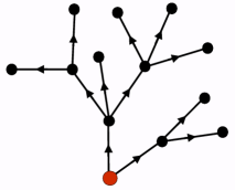
Figure 2: A tree with $K^{+}$ edges.

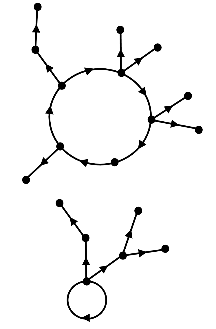
(a) $K^{+}$ loops

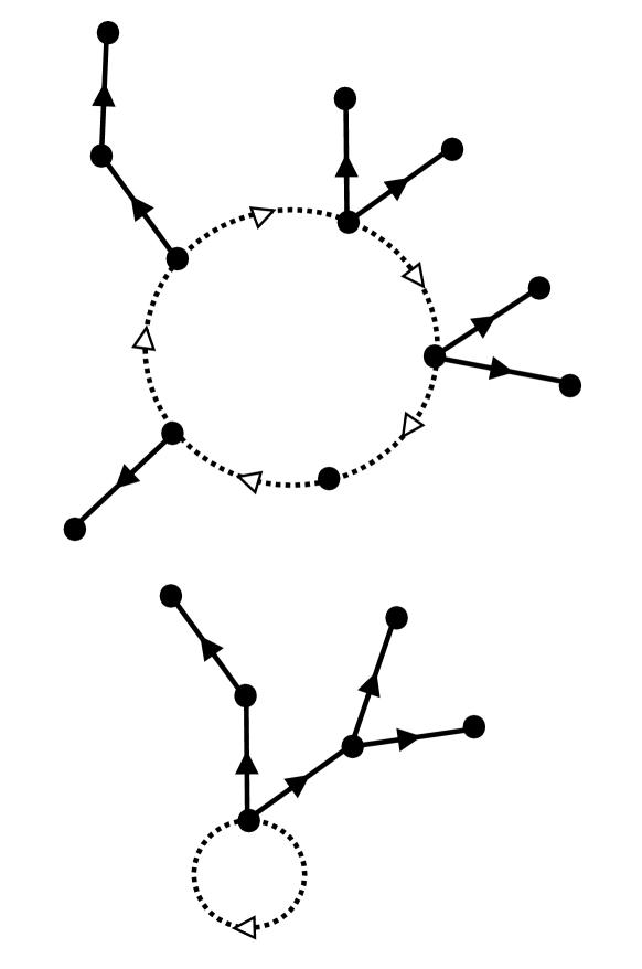
(b) $K^{-}$ loops

Figure 3: Examples of loops with out-growing trees. $K^{-}$ propagators are drawn as dashed lines. They appear only in a loop and such loop comes with a factor of $-1$. Tadpoles are loops of length $1$.

• A rooted directed tree with only positive edges $\ell_{kl}^{+}=\langle v_{k}\to v_{l}\rangle^{+}$ oriented so that the edge points to the vertex which is farther from the root, as shown in fig. 3. The weight of such a tree is a product of a factor $r_{j}D_{ab}(u_{j})$ associated with the root $v_{j}$ and factors $r_{l}r_{k}K^{+}_{lk}$ associated with its edges $\ell_{kl}^{+}$.

• A positive (fig. 3(a)) or a negative (fig. 3(b)) oriented cycle with outgrowing trees. A positive/negatice loop is an oriented cycle (including tadpoles which are cycles of length 1) entirely made of positive/negative edges having the same orientation. The outgrowing trees consist of positive edges only. The weight of a loop with outgrowing trees is the product of the weights of its edges, with the weight of an edge $\ell_{kl}^{\pm}$ given by $r_{l}r_{k}K^{\pm}_{lk}$. In addition, a negative loop carries an extra minus sign. This is why we will call the positive loops bosonic and the negative loops fermionic.

Summarising, we write the determinant of the matrix (4.2) as

$$\begin{split}\det\hat{G}_{jk}&=\sum_{\cal F}W[{\cal F}],\\ W[{\cal F}]&=(-1)^{\#\text{negative loops}}\prod_{v_{j}\in\text{roots}}r_{j}D_{ab}(u_{j})\ \prod_{\ell_{kl}^{\pm}\in\text{edges}}r_{l}r_{k}K^{\pm}(u_{l},u_{k}),\end{split}$$ (4.3)

with $K^{\pm}(u,v)=K(u,v)\pm K(u,-v)$. Equation (4.3) allows us to express the Jacobian for the integration measure as a sum over graphs whose weights depend only on the “coordinates” $\{u_{j},r_{j}\}$ of its vertices. For a periodic system $K^{+}=K^{-}$ and the two families of loops cancel each other, leaving only trees in the expansion of the Gaudin matrix [9].

4.2 Graph expansion of the partition function

Applying the matrix-tree theorem for each term in the series (3.14), we obtain a graph expansion for the partition function

$$Z_{ab}(R,L)=\sum_{m=0}^{\infty}\frac{(-1)^{m}}{m!}\sum_{1\leq r_{1},...,r_{m}}\prod_{j=1}^{m}\int_{0}^{\infty}\frac{du_{j}}{2\pi}\frac{(-1)^{r_{j}}}{r_{j}^{2}}e^{-r_{j}RE(u_{j})}\sum_{{\cal F}}W[{\cal F}],$$ (4.4)

where the last sum runs over all graphs ${\cal F}$ with $m$ vertices as constructed above.

The next step is to invert the order of the sum over graphs and the integral/sum over the coordinates $\{u_{j},r_{j}\}$ assigned to the vertices. As a result we obtain a sum over the ensemble of abstract oriented tree/loop graphs, with their symmetry factors, embedded in the space $\mathbb{R}^{+}\times\mathbb{N}$ where the coordinates $u,r$ of the vertices take values. The embedding is free, in the sense that the sum over the positions of the vertices is taken without restriction. As a result, the sum over the embedded graphs is the exponential of the sum over connected ones. One can think of these graphs as Feynman diagrams obtained by applying the Feynman rules in Fig. 4.

The Feynman rules comprise there kinds of vertices: "root" vertices with only outgoing bosons, "bosonic" vertices with one incoming boson and an arbitrary number of outgoing bosons, "fermionic" vertices with one incoming and one outgoing fermion, together with an arbitrary number of outgoing bosons. The connected diagrams built from these vertices are either trees (figure 3) or bosonic loops (fig. 3(a)) or fermionic loops (fig. 3(b)).

The free energy is a sum over these graphs,

$$\log Z_{ab}(R,L)=\int_{0}^{\infty}\frac{du}{2\pi}D_{ab}(u)\sum_{r\geq 1}rY_{r}(u)+\sum_{n\geq 1}\mathcal{C}^{\pm}_{n}.$$ (4.5)

In this expression, $Y_{r}(u)$ denotes the sum of over all trees rooted at the point $(u,r)$ and $\mathcal{C}^{\pm}_{n}$ is the sum over the Feynman graphs having a bosonic/fermionic loop of length $n$. We have defined $Y_{r}(u)$ in such a way that the all vertices with $r$ outgoing lines, including the root, have the same weight.

$$\boxed{\begin{split}\vbox{\hbox{\includegraphics[height=38.74988pt]{rootf}}}\ \qquad&=\ \ \ rD_{ab}(u){(-1)^{r-1}\over r^{2}}\ e^{-rRE(u)}\\ \vbox{\hbox{\includegraphics[height=38.74988pt]{vertexboson}}}\quad=\quad\vbox{\hbox{\includegraphics[height=38.74988pt]{vertexfermion}}}\ \qquad&=\ \ \ {(-1)^{r-1}\over r^{2}}\ e^{-rRE(u)}\\ \vbox{\hbox{\includegraphics[height=25.83325pt]{boson}}}\ \quad&=\ \ \ r_{1}r_{2}K^{+}(u_{2},u_{1})\\ \vbox{\hbox{\includegraphics[height=25.83325pt]{fermion}}}\ \quad&=\ \ \ r_{1}r_{2}K^{-}(u_{2},u_{1})\\ \vbox{\hbox{\includegraphics[height=47.36096pt]{fermionloop}}}\quad&=\ \ \ -1\end{split}}$$

Figure 4: The Feynman rules for the partition function. The vertex labeled by $(u,r)$ has $r$ outgoing lines.

5 Summing up the connected graphs: the exact $g$-function

5.1 The tree contribution

In this section, we analyze the part of free energy (4.5) that comes from the tree-diagrams

$$\log Z_{ab}(R,L)^{\textnormal{trees}}=\int_{0}^{+\infty}\frac{du}{2\pi}D_{ab}(u)\sum_{r\geq 1}rY_{r}(u),$$ (5.1)

$$\text{where}\quad Y_{r}(u)=\sum\vbox{\hbox{\includegraphics[width=71.13188pt]{Ydefinition}}}\;\equiv\vbox{\hbox{\includegraphics[width=19.91684pt]{blob}}}.$$ (5.2)

Being the generating function for directed trees rooted at $(u,r)$, $Y_{r}(u)$ obeys a simple equation

$$Y_{r}(u) =\frac{(-1)^{r-1}}{r^{2}}e^{-rRE(u)}\sum_{n=0}^{\infty}\frac{1}{n!}\bigg{(}\sum_{s=1}^{\infty}\int_{0}^{+\infty}\frac{dv}{2\pi}srK^{+}(v,u)Y_{s}(v)\bigg{)}^{n}$$

$$=\frac{(-1)^{r-1}}{r^{2}}\bigg{[}e^{-RE(u)}\exp\sum_{s=0}^{\infty}\int_{0}^{+\infty}\frac{dv}{2\pi}K^{+}(v,u)sY_{s}(v)\bigg{]}^{r},$$ (5.3)

This equation can be understood diagramatically as in figure 5.

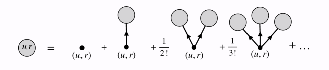
Figure 5: The combinatorial structure of trees with a fixed root.

In particular, we have for $r=1$

$$Y_{1}(u)=e^{-RE(u)}\exp\sum_{s=0}^{\infty}\int_{0}^{+\infty}\frac{dv}{2\pi}K^{+}(v,u)sY_{s}(v).$$ (5.4)

By replacing (5.4) into (5.3), we can express $Y_{r}$ in terms of $Y_{1}$ for arbitrary $r\geq 1$

$$Y_{r}(u)=\frac{(-1)^{r-1}}{r^{2}}Y_{1}(u)^{r}.$$ (5.5)

This allows us to rewrite (5.4) as a closed equation for $Y_{1}$

$$Y_{1}(u)=e^{-RE(u)}\exp\int_{0}^{+\infty}\frac{dv}{2\pi}K^{+}(v,u)\log[1+Y_{1}(v)].$$

This integral can be extended to the real axis by using the parity of the kernel $K^{+}(v,u)=K(v,u)+K(-v,u)$ and by defining $Y_{1}(-u)=Y_{1}(u)$

$$Y_{1}(u)=e^{-RE(u)}\exp\int_{-\infty}^{+\infty}\frac{dv}{2\pi}K(v,u)\log[1+Y_{1}(v)],$$

This is nothing but the TBA equation for a periodic system at inverse temperature $R$. In particular, the periodic partition function can be written in terms of $Y_{1}$

$$\log Z(R,L)=L\int_{-\infty}^{+\infty}\frac{du}{2\pi}p^{\prime}(u)\log[1+Y_{1}(u)].$$ (5.6)

Similarly, we can also extend the domain of integration in (5.2) to the real axis, using the parity of $D_{ab}(u,r)$ and $Y_{1}$. By subtracting the periodic free energy (5.6) from the tree part of the free energy (5.2), we obtain the tree contribution to $g$-function

$$\mathcal{F}_{ab}(R)^{\textnormal{trees}}=\frac{1}{2}\int_{-\infty}^{+\infty}\frac{du}{2\pi}[\Theta_{a}(u)+\Theta_{b}(u)]\log[1+Y_{1}(u)].$$ (5.7)

5.2 Loop contribution

Now we turn to the sum over loops and show that they fill the missing part [5] of the $g$-function (2.13). Let us define

$$\mathcal{F}_{ab}(R,L)^{\textnormal{loops}}=\sum_{n\geq 1}\mathcal{C}_{n}^{\pm}.$$ (5.8)

For each $n\geq 1$, $\mathcal{C}_{n}^{\pm}$ is the partition sum of $K^{\pm}$ loops of length $n$ with the trees growing out of these loops which can be summed separately

$$\mathcal{C}_{n}^{\pm}=\frac{\pm 1}{n}\sum_{1\leq r_{1},...,r_{n}}\int\limits_{0}^{\infty}\frac{du_{1}}{2\pi}...\int\limits_{0}^{\infty}\frac{du_{n}}{2\pi}Y_{r_{1}}(u_{1})....Y_{r_{n}}(u_{n})r_{2}r_{1}K^{\pm}(u_{2},u_{1})....r_{1}r_{n}K^{\pm}(u_{1},u_{n}).$$

In this expression, the sign comes from fermion loop and $1/n$ is the usual loop symmetry factor.

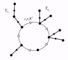
Figure 6: A $K^{-}$ loop connecting $n$ points $(u_{j},r_{j})$. Trees growing out of a vertex $(u_{j},r_{j})$ sum up to the corresponding $Y_{r}(u)$ function. The factor $r_{j-1}r_{j}$ of the propagator from $(u_{j-1},r_{j-1})$ to $(u_{j},r_{j})$ can be pulled into the adjacent trees. Taking the sum over all $r_{j}$ results in the Fermi-Dirac factor $Y_{1}(u_{j})/(1+Y_{1}(u_{j}))$ at each vertex $j$.

We can use the relation (5.5) to carry out the sum over $r$

$$\sum_{r\geq 1}r^{2}Y_{r}(u)=\frac{Y_{1}(u)}{1+Y_{1}(u)}.$$

It follows that

$$\mathcal{C}_{n}^{\pm}=\frac{\pm 1}{n}{\rm tr}(\hat{K}^{\pm})^{n}.$$ (5.9)

where the kernels $\hat{K}^{\pm}$ are defined in (2.15). The loop contribution is therefore given by

$$\mathcal{F}_{ab}(R)^{\textnormal{loops}}=\log\det\frac{1-\hat{K}^{-}}{1-\hat{K}^{+}}.$$ (5.10)

The $g$-function is obtained by combining (5.7) and (5.10) and set $a=b$

$$\log g_{a}(R)= \frac{1}{2}\big{[}\mathcal{F}_{aa}^{\textnormal{trees}}(R)+\mathcal{F}_{aa}^{\textnormal{loops}}(R)\big{]}$$

$$= \frac{1}{2}\int_{-\infty}^{+\infty}\frac{du}{2\pi}\Theta_{a}(u)\log[1+Y_{1}(u)]+\frac{1}{2}\log\det\frac{1-\hat{K}^{-}}{1-\hat{K}^{+}}.$$ (5.11)

5.3 Excited state g-function

In this section, we derive the excited state g-function. This quantity can be regarded as the normalized overlap between the boundary state and an excited bulk eigenstate

$$g_{a}^{\psi}=\frac{\langle B_{a}|\psi\rangle}{\sqrt{\langle\psi|\psi\rangle}}.$$ (5.12)

By setting $|\psi\rangle$ to the ground state $|\psi_{0}\rangle$, we recover the definition (2.10) of the g-function. We restrict our computation to the case where $|\psi\rangle$ is of the form $|\pm w_{1},\pm w_{2},...,\pm w_{N}\rangle$. We also assume for simplicity that the scattering matrix is a function of the difference of rapidities (relativistic invariance).

First, let us briefly summarize the excited state TBA equations for a periodic system, following [9]. We consider a torus with one large dimension $L$ (physical volume) and a finite dimension $R$ (mirror volume). A mirror state $|\vartheta\rangle=|v_{1},...,v_{N}\rangle$ propagates along the $L$ direction. Note that the mirror-physics convention is in reverse order compared to [9]. The Boltzmann weight of a physical particle is dressed by the interaction with these mirror particles

$$Y_{\vartheta}^{\circ}(u)=e^{-RE(u)}\prod_{j=1}^{N}S(u-v_{j}+i\pi/2),$$ (5.13)

To compute the energy of the mirror state $|\vartheta\rangle$, we have to add to the free energy the contribution from the mirror particles that go directly to the opposite edge without scattering

$$E(\vartheta)=-\frac{1}{L}\log Z(R,L,\vartheta)=\sum_{j=1}^{N}{E}(v_{j})-\int_{-\infty}^{+\infty}\frac{du}{2\pi}p^{\prime}(u)\log(1+Y_{\vartheta}(u)),$$ (5.14)

where $Y_{\vartheta}$ solves for the excited state TBA equation

$$Y_{\vartheta}(u)=Y_{\vartheta}^{\circ}(u)\exp\big{[}\int_{-\infty}^{+\infty}\frac{dw}{2\pi}K(w,u)\log(1+Y_{\vartheta}(w))\big{]}.$$ (5.15)

The on-shell condition for the state $|\vartheta\rangle$ is obtained by transforming a mirror particle of rapidity $v_{j}$ to a physical particle of rapidity $v_{j}-i\pi/2$. The relative factor between the two ways of computing the partition function is $-Y(v_{j}-i\pi/2)$. This leads to the finite volume Bethe equations

$$Y(v_{j}-i\pi/2)=-1,\quad j=1,2,...,N.$$ (5.16)

Now let us return to the excited state g-function (5.12). We repeat the same exercise for a long cylinder of length $L$ and radius $R$ with two boundaries $a$ and $b$ together with a state $|\psi\rangle=|\pm w_{1},\pm w_{2},...,\pm w_{N}\rangle$ propagating in the $L$ direction. We denote the partition function in this case by $Z_{ab}(R,L,\psi)$.

The idea is, if we can identify the excited energy (5.14) with the extensive part of the partition function $Z_{ab}(R,L,\psi)$ when $|\psi\rangle\equiv|\vartheta\rangle$, then the rest (intensive part) gives us the excited g-function corresponding to $|\psi\rangle$

$$g_{a}^{\psi}g_{b}^{\psi}=\frac{Z_{ab}(R,L,\psi)}{Z(R,L,\psi)}.$$ (5.17)

To compute $Z_{ab}(R,L,\psi)$ we perform the sum over eigenstates of the physical Hamiltonian with boundary $H_{ab}$. The procedure is similar to that of ground-state g-function: we obtain a sum over trees and loops. The only difference is the Feynman rule for the vertices

$$e^{-RE(u)}\to e^{-RE(u)}\prod_{j=1}^{N}S(u-w_{j}+i\pi/2)S(u+w_{j}+i\pi/2)\equiv\tilde{Y}_{\psi}^{\circ}(u)$$ (5.18)

In particular, the extensive part of the partition function $Z_{ab}(R,L,\psi)$ is given by

$$\log Z_{ab}(R,L,\psi)^{\textnormal{extensive}}=-L\sum_{j=1}^{N}{E}(\pm w_{j})+2L\int_{0}^{\infty}\frac{du}{2\pi}p^{\prime}(u)\log(1+\tilde{Y}_{\psi}(u))$$ (5.19)

where $\tilde{Y}_{\psi}(u)$ being the sum of trees rooted at vertex $u$ now satisfies the equation

$$\tilde{Y}_{\psi}(u)=\tilde{Y}_{\psi}^{\circ}(u)\exp\big{[}\int_{0}^{+\infty}\frac{dw}{2\pi}K^{+}(w,u)\log(1+\tilde{Y}_{\psi}(w))\big{]}.$$ (5.20)

As a consequence of the crossing symmetry $S(u)=S(i\pi-u)$ we have the identity

$$S(u-w_{j}+i\pi/2)S(u+w_{j}+i\pi/2)=S(-u-w_{j}+i\pi/2)S(-u+w_{j}+i\pi/2)$$ (5.21)

which means that the function $\tilde{Y}_{\psi}^{\circ}(u)$ is an even function of $u$. Therefore we can extend $\tilde{Y}_{\psi}$ to the real axis and identify $\tilde{Y}_{\psi}$ with $Y_{\vartheta}$ when $|\psi\rangle=|\vartheta\rangle$. Again we have $\tilde{Y}_{\psi}(w_{j})=\tilde{Y}_{\psi}(-w_{j})=-1$. We conclude that

$$\log(g_{a}^{\psi}g_{b}^{\psi})(R)=\int_{0}^{\infty}\frac{du}{2\pi}[\Theta_{a}(u)+\Theta_{b}(u)]\log(1+\tilde{Y}_{\psi}(u))+\log\det\frac{1-\hat{K}^{-}_{\psi}}{1+\hat{K}^{+}_{\psi}},$$ (5.22)

where the Fermi-Dirac factor in the kernel $\hat{K}^{\pm}_{\psi}$ is now given by $\tilde{Y}_{\psi}/(1+\tilde{Y}_{\psi})$, c.f. eq. (2.15).

Our method produces correctly equations (5.15), (5.16), (5.20) that determine the excited states in both periodic and open case. However in the periodic case our intuitive picture misses a contribution $\sum E(v_{j})$ to the excited state energy. Similarly, we believe that the structure of the excited state g-function given in (5.22) is correct up to a simple additional contribution. By comparison with the asymptotic g-function derived in [14], this term appears to be the mirror-continued reflection factor. We leave this problem to future investigations.

6 More than one type of particle

In this section we generalize our method to theories with multiple species of particle interacting via diagonal bulk scattering and diagonal reflection matrices. This generalization also provides insight on g-function of non-diagonal theories solved by Nested Bethe Ansatz. We present a regularization scheme for these theories and we consider an explicit example in another work [13].

For simplicity we consider a theory with two species. The bulk scattering matrices and the reflection matrices are denoted by $S_{pq}$ and $R_{pa},R_{pb}$ for $p,q\in\{1,2\}$. They are assumed to satisfy the following properties

$$S_{pp}(u,u)=-1,$$

$$S_{pq}(u,v)S_{qp}(v,u)=R_{pa}(u)R_{pa}(-u)=R_{pb}(u)R_{pb}(-u)=1,$$ (6.1)

$$S_{pq}(u,-v)S_{qp}(-u,v)=1.$$

The last property is only needed for system with boundaries.

6.1 Periodic systems

An $(N_{1}+N_{2})$-particle state is characterized by a set of rapidities $|u_{11},...,u_{1N_{1}},u_{21},...,u_{2N_{2}}\rangle$. Particles of the same type must have different rapidities: $u_{1j}\neq u_{1k}$, $u_{2j}\neq u_{2k}$. The Bethe equations for such state read

$$p_{1}(u_{1j})L+\sum_{k\neq j}^{N_{1}}-i\log S_{11}(u_{1j},u_{1k})+\sum_{k=1}^{N_{2}}-i\log S_{12}(u_{1j},u_{2k})=\phi_{1j}=2\pi n_{1j},$$ (6.2)

$$p_{2}(u_{2j})L+\sum_{k=1}^{N_{1}}-i\log S_{21}(u_{2j},u_{1k})+\sum_{k\neq j}^{N_{2}}-i\log S_{22}(u_{2j},u_{2k})=\phi_{2j}=2\pi n_{2j}.$$

The partition function can be written as a sum runs over two sets of mode numbers $\textbf{n}_{1}=n_{11},...,n_{1m_{1}}$ and $\textbf{n}_{2}=n_{21},...,n_{2m_{2}}$ along with two sets of multiplicities (wrapping numbers) $\textbf{r}_{1}=r_{11},...,r_{1m_{1}}$ and $\textbf{r}_{2}=r_{21},...,r_{2m_{2}}$

$$Z_{ab}(R,L)=\sum_{\begin{subarray}{c}m_{1}=0\\ m_{2}=0\end{subarray}}^{\infty}\frac{(-1)^{m_{1}+m_{2}}}{m_{1}!m_{2}!}\;\sum_{\begin{subarray}{c}0\leq\textbf{n}_{1},\textbf{n}_{2}\\ 1\leq\textbf{r}_{1},\textbf{r}_{2}\end{subarray}}\;\prod_{p=1}^{2}\prod_{j=1}^{m_{p}}\frac{(-1)^{r_{pj}}}{r_{pj}}e^{-RE((\textbf{n}_{1},\textbf{r}_{1}),(\textbf{n}_{2},\textbf{r}_{2}))}.$$ (6.3)

The mode numbers $((\textbf{n}_{1},\textbf{r}_{1}),(\textbf{n}_{2},\textbf{r}_{2}))$ are related to the rapidities $((\textbf{u}_{1},\textbf{r}_{1}),(\textbf{u}_{2},\textbf{r}_{2}))$ through Bethe equations with multiplicities

$$p_{1}(u_{1j})L+\sum_{k\neq j}^{m_{1}}-ir_{1k}\log S_{11}(u_{1j},u_{1k})+\sum_{k=1}^{m_{2}}-ir_{2k}\log S_{12}(u_{1j},u_{2k})=\phi_{1j}=2\pi n_{1j},$$

$$p_{2}(u_{2j})L+\sum_{k=1}^{m_{1}}-ir_{1k}\log S_{21}(u_{2j},u_{1k})+\sum_{k\neq j}^{m_{2}}-ir_{2k}\log S_{22}(u_{2j},u_{2k})=\phi_{2j}=2\pi n_{2j}.$$

The Gaudin matrix has a $2\times 2$ block structure

$$\hat{G}=\begin{pmatrix}\textbf{r}_{1}\partial_{u_{1}}\phi_{1}&\textbf{r}_{1}\partial_{u_{2}}\phi_{1}\\ \textbf{r}_{2}\partial_{u_{1}}\phi_{2}&\textbf{r}_{2}\partial_{u_{2}}\phi_{2}\end{pmatrix}^{t}=\begin{pmatrix}\hat{A}&\hat{B}\\ \hat{C}&\hat{D}\end{pmatrix}$$ (6.4)

The explicit expressions of each block are

$$\hat{A}_{jk}=\delta_{jk}[r_{1j}Lp^{\prime}_{1j}+\sum_{l\neq j}^{m_{1}}r_{1j}r_{1l}K_{11}^{jl}+\sum_{l=1}^{m_{2}}r_{1j}r_{2l}K_{12}^{jl}]-r_{1j}r_{1k}K_{11}^{jk},$$

$$\hat{B}_{jk}=-r_{1j}r_{2k}K_{12}^{jk},\quad\hat{C}_{jk}=-r_{2j}r_{1k}K_{21}^{jk},$$

$$\hat{D}_{jk}=\delta_{jk}[r_{2j}Lp^{\prime}_{2j}+\sum_{l=1}^{m_{1}}r_{2j}r_{1l}K_{21}^{jl}+\sum_{l\neq j}^{m_{2}}r_{2j}r_{2l}K_{22}^{jl}]-r_{2j}r_{2k}K_{22}^{jk}.$$

The partition function can be written in terms of the determinant of this matrix

$$Z(R,L)=\sum_{\begin{subarray}{c}m_{1}=0\\ m_{2}=0\end{subarray}}^{\infty}\frac{1}{m_{1}!m_{2}!}\sum_{\textbf{r}_{1},\textbf{r}_{2}}\prod_{p=1}^{2}\prod_{j=1}^{m_{p}}\int_{-\infty}^{+\infty}\frac{du_{pj}}{2\pi}\frac{(-1)^{r_{pj}-1}}{r_{pj}^{2}}e^{-r_{pj}RE_{p}(u_{pj})}\det\hat{G}.$$ (6.5)

We apply the matrix-tree theorem for the matrix $\hat{G}$ and obtain a tree expansion of the free energy. Each vertex now carries an index $p\in\{1,2\}$ to indicate what type of particle it stands for. A branch going from vertex of type $p$ to vertex of type $q$ has a weight of $r_{q}r_{p}K_{qp}$. We represent vertices of type 1 by a disk and those of type 2 by a circle.

Let us denote by $Y_{pr}(u)$ the sum over all the trees rooted at $(u,r)$ of type $p$. The free energy is given by

$$\log Z(R,L)=L\int_{-\infty}^{+\infty}\frac{du}{2\pi}\bigg{[}p_{1}^{\prime}(u)\sum_{r}rY_{1r}(u)+p_{2}^{\prime}(u)\sum_{r}Y_{2r}(u)\bigg{]}.$$ (6.6)

$$\boxed{\begin{split}\vbox{\hbox{\includegraphics[height=43.05542pt]{su31vertex}}}\ \quad&=\ \ \ {(-1)^{r_{1}-1}\over r_{1}^{2}}\ e^{-r_{1}RE_{1}(u)}\\ \vbox{\hbox{\includegraphics[height=45.20819pt]{su32vertex}}}\ \quad&=\ \ \ {(-1)^{r_{2}-1}\over r_{2}^{2}}\ e^{-r_{2}RE_{2}(u)}\end{split}}$$ (6.7)

The generating functions of the two types of trees are intertwined with each other

$$Y_{1r}(u) =\frac{(-1)^{r-1}}{r^{2}}e^{-rRE_{1}(u)}\exp\bigg{[}r\int\frac{dv}{2\pi}\sum_{s}sK_{11}(v,u)Y_{1s}(v)+sK_{21}(v,u)Y_{2s}(v)\bigg{]},$$

$$Y_{2r}(u) =\frac{(-1)^{r-1}}{r^{2}}e^{-rRE_{2}(u)}\exp\bigg{[}r\int\frac{dv}{2\pi}\sum_{s}sK_{12}(v,u)Y_{1s}(v)+sK_{22}(v,u)Y_{2s}(v)\bigg{]}.$$

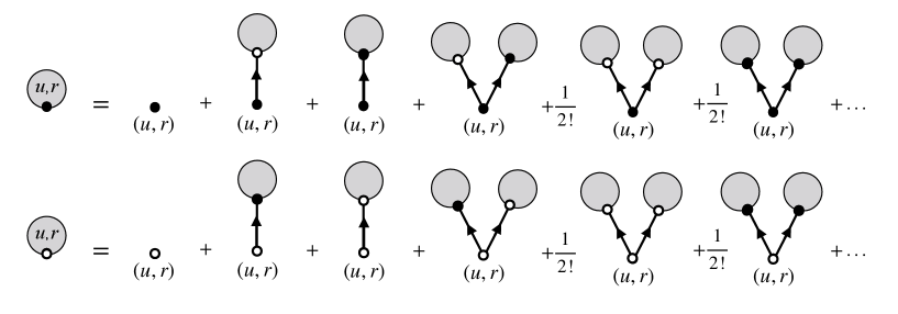
Figure 7: The two-species TBA equations

In particular, we have

$$Y_{1r}(u)=\frac{(-1)^{r-1}}{r^{2}}Y^{r}_{11}(u),\quad Y^{r}_{2r}(u)=\frac{(-1)^{r-1}}{r^{2}}Y^{r}_{21}(u).$$ (6.8)

For simplicity, let us denote $Y_{11}$ and $Y_{21}$ simply by $Y_{1}$ and $Y_{2}$. We recover the TBA equation of two species

$$\log Z(R,L) =L\int_{-\infty}^{+\infty}\frac{du}{2\pi}\bigg{\{}p_{1}^{\prime}(u)\log[1+Y_{1}(u)]+p_{2}^{\prime}(u)\log[1+Y_{2}(u)]\bigg{\}},$$ (6.9)

$$Y_{1}(u) =e^{-RE_{1}(u)}\exp\big{[}K_{11}\star\log(1+Y_{1})+K_{21}\star\log(1+Y_{2})\big{]},$$

$$Y_{2}(u) =e^{-RE_{2}(u)}\exp\big{[}K_{12}\star\log(1+Y_{1})+K_{22}\star\log(1+Y_{2})\big{]}.$$

6.2 Open systems

Let us denote by $R_{1ab}$ and $R_{2ab}$ the reflection factors of the first and second particle.The Bethe equations for the state $|u_{11},...,u_{1N_{1}},u_{21},...,u_{2N_{2}}\rangle$ now read

$$e^{2ip_{1}(u_{1j})L}R_{1ab}(u_{1j})\prod_{k\neq j}^{N_{1}}S_{11}(u_{1j},u_{1k})S_{11}(u_{1j},-u_{1k})\prod_{k=1}^{N_{2}}S_{12}(u_{1j},u_{2k})S_{12}(u_{1j},-u_{2k})=1,$$

$$e^{2ip_{2}(u_{2j})L}R_{2ab}(u_{2j})\prod_{k=1}^{N_{1}}S_{21}(u_{2j},u_{1k})S_{21}(u_{2j},-u_{1k})\prod_{k\neq j}^{N_{2}}S_{22}(u_{2j},u_{2k})S_{22}(u_{2j},-u_{2k})=1.$$

The rapidities and the mode numbers are taken to be positive. Similar to (3.6), we have

$$Z_{ab}(R,L)=\sum_{\begin{subarray}{c}m_{1}=0\\ m_{2}=0\end{subarray}}^{\infty}\frac{(-1)^{m_{1}+m_{2}}}{m_{1}!m_{2}!}\;\sum_{\begin{subarray}{c}0\leq\textbf{n}_{1},\textbf{n}_{2}\\ 1\leq\textbf{r}_{1},\textbf{r}_{2}\end{subarray}}\;\prod_{p=1}^{2}\prod_{j=1}^{m_{p}}\frac{(-1)^{r_{pj}}}{r_{pj}}(1-\delta_{n_{pj},0})e^{-RE((\textbf{n}_{1},\textbf{r}_{1}),(\textbf{n}_{2},\textbf{r}_{2}))}.$$ (6.10)

The conversion between mode numbers and rapidities under the presence of multiplicities

$$2p_{1}(u_{1j})L-i\log\bigg{[}R_{1ab}(u_{1j})[\mathbb{S}_{11}(u_{1j},u_{1j})]^{r_{1j}-1}\prod_{k\neq j}^{m_{1}}[\mathbb{S}_{11}(u_{1j},u_{1k})]^{r_{1k}}\prod_{k=1}^{m_{2}}[\mathbb{S}_{12}(u_{1j},u_{2k})]^{r_{2k}}\bigg{]} =\phi_{1j}$$

$$2p_{2}(u_{2j})L-i\log\bigg{[}R_{2ab}(u_{2j})[\mathbb{S}_{22}(u_{2j},u_{2j})]^{r_{2j}-1}\prod_{k=1}^{m_{1}}[\mathbb{S}_{21}(u_{2j},u_{1k})]^{r_{1k}}\prod_{k\neq j}^{m_{2}}[\mathbb{S}_{22}(u_{2j},u_{2k})]^{r_{2k}}\bigg{]} =\phi_{2j}$$

where we have used the notation $\mathbb{S}_{pq}(u,v)=S_{pq}(u,v)S_{pq}(u,-v)$. The Gaudin matrix now has a $2\times 2$ block structure

$$\hat{G}_{ab}=\begin{pmatrix}r_{1}[\partial_{u_{1}}\phi_{1}-2\pi\delta(u_{1})]&r_{1}\partial_{u_{2}}\phi_{1}\\ r_{2}\partial_{u_{1}}\phi_{2}&r_{2}[\partial_{u_{2}}\phi_{2}-2\pi\delta(u_{2})]\end{pmatrix}^{t}=\begin{pmatrix}\hat{A}&\hat{B}\\ \hat{C}&\hat{D}.\end{pmatrix}$$ (6.11)

The explicit expressions of each block are

$$\hat{A}_{jk}=\delta_{jk}\bigg{[}r_{1j}[2Lp_{1}^{\prime}(u_{1j})+\Theta_{1ab}(u_{1j})]+r_{1j}^{2}(K_{11}^{jj+}-K_{11}^{jj-})+\sum_{l\neq j}^{n}r_{1j}r_{1l}K_{11}^{jl+}+\sum_{l=1}^{m}r_{1j}r_{2l}K_{12}^{jl+}\bigg{]}$$

$$\qquad\qquad\qquad\qquad\qquad\qquad\qquad\qquad\qquad-r_{1j}r_{1k}K_{11}^{jk-},$$

$$\hat{B}_{jk}=-r_{1j}r_{2k}K_{12}^{jk-},\quad\hat{C}_{jk}=-r_{2j}r_{1k}K_{21}^{jk-},$$

$$\hat{D}_{jk}=\delta_{jk}\bigg{[}r_{2j}[2Lp_{2}^{\prime}(u_{1j})+\Theta_{2ab}(u_{2j})]+r_{2j}^{2}(K_{22}^{jj+}-K_{22}^{jj-})+\sum_{l=1}^{m}r_{2j}r_{1l}K_{21}^{jl+}+\sum_{l\neq j}^{m}r_{2j}r_{2l}K_{22}^{jl+}\bigg{]}$$

$$\qquad\qquad\qquad\qquad\qquad\qquad\qquad\qquad\qquad-r_{2j}r_{2k}K_{22}^{jk-}.$$

where the notations are

$$\Theta_{pab}=\Theta_{pa}+\Theta_{pb},\quad\Theta_{p\star}(u)=K_{p\star}(u)-K_{pp}(u,-u)-\pi\delta(u),\;\star=a,b$$

$$K_{pq}^{jk\pm}=K_{pq}(u_{pj},u_{qk})\pm K_{pq}(u_{pj},-u_{qk}),\quad\textnormal{for }p,q\in\{1,2\}.$$

If we set $\Theta$ to zero and $K^{+}$ and $K^{-}$ to equal then we would recover the Gaudin matrix for the periodic system (6.4). The partition function is written in terms of the determinant of this matrix

$$Z_{ab}(R,L)=\sum_{\begin{subarray}{c}m_{1}=0\\ m_{2}=0\end{subarray}}\frac{1}{m_{1}!m_{2}!}\sum_{1\leq\textbf{r}_{1},\textbf{r}_{2}}\prod_{p=1}^{2}\prod_{j=1}^{m_{p}}\int_{-\infty}^{+\infty}\frac{du_{pj}}{2\pi}\frac{(-1)^{r_{pj}-1}}{r_{pj}^{2}}e^{-r_{pj}RE_{p}(u_{pj})}\det\hat{G}_{ab}.$$ (6.12)

The tree contribution to $g$-function is obtained in a similar way as before

$$\log(g_{a}g_{b})^{\textnormal{trees}}(R)=\frac{1}{2}\sum_{p=1}^{2}\int_{-\infty}^{+\infty}\frac{du}{2\pi}\Theta_{pab}(u)\log(1+Y_{p}(u)),$$ (6.13)

where $Y_{p}$ for $p=1,2$ are solutions of the TBA equations (6.9).

Now comes the loop contribution

$$\log(g_{a}g_{b})^{\textnormal{loops}}(R)=\sum_{n\geq 1}\mathcal{C}^{\pm}_{n},$$ (6.14)

where $\mathcal{C}^{\pm}_{n}$ denotes the sum over bosonic/fermionic loops of length $n$. Each of these $n$ vertices can be either of type 1 or 2. The trees growing out of each vertex can be summed to the Fermi-Dirac factor of each type, by virtue of the relation (6.8)

$$\sum_{r}r^{2}Y_{pr}(u)=\frac{Y_{p}(u)}{1+Y_{p}(u)}=f_{p}(u),\quad p=1,2.$$ (6.15)

The loop contribution can then be written as a sum over cyclic sets p of $\mathfrak{C}(\{1,2\}^{n})$

$$\mathcal{C}^{\pm}_{n}=\pm\sum_{p_{1},...,p_{n}\in\mathfrak{C}(\{1,2\}^{n})}\frac{1}{S(\textbf{p})}\prod_{j=1}^{n}\int_{0}^{+\infty}\frac{du_{j}}{2\pi}f_{p_{j}}(u_{j})K^{\pm}_{p_{2}p_{1}}(u_{2},u_{1})....K^{\pm}_{p_{1}p_{n}}(u_{1},u_{n}),$$ (6.16)

where $S(\textbf{p})$ is the symmetry factor of p. This sum is nothing but the trace of $2\times 2$ matrices $\hat{K}^{\pm}$ with elements

$$K^{\pm}_{pq}(F)(u)=\int_{0}^{+\infty}\frac{dv}{2\pi}K^{\pm}_{pq}(u,v)f_{q}(v)F(v),\quad p,q\in\{1,2\}.$$

We obtain two Fredholm determinants with $2\times 2$ matrix kernels as a generalization of (5.10)

$$\log(g_{a}g_{b})^{\textnormal{loops}}(R)=\log\det\frac{1-\hat{K}^{-}}{1-\hat{K}^{+}}.$$ (6.17)

6.3 g-function of theories with non-diagonal bulk scattering

A periodic theory with non-diagonal bulk scattering can be diagonalized with the Nested Bethe Ansatz technique. The Bethe equations then involve additional particles with vanishing momentum and energy. These particles called magnons can be regarded as excitations on a spin chain where the physical rapidities are non-dynamical impurities. In particular the number of magnons cannot exceed the number of physical particles. This constraint presents a major obstruction in the implementation of our approach for non-diagonal theories as we cannot carry out the first step of summing over mode numbers.

When the number of physical particles is large however, magnons can form strings of evenly distributed complex rapidities. As a consequent, the TBA equations are effectively the same as those of a diagonal theories with an infinite number of particles in the spectrum. This means that if we include magnon strings into our cluster expansion and remove the constraint of their numbers, then according to the above analysis we will recover the correct TBA equations.

If we follow this line of logic to non-diagonal open systems, we come to the conclusion that the g-function of these theories is an infinite-dimensional extension of (6.13) and (6.17). Such direct extension proves however to be problematic. Indeed, as magnons have vanishing energy, there is no driving term in the TBA equations determining their pseudo-energies. As a consequent, the corresponding Y-functions do not vanish at zero temperature limit and so does the g-function. This value of g-function at zero temperature comes from graphs made entirely of magnons. Their contribution is present at any temperature and we propose to get rid of it by normalizing the finite temperature g-function by its zero temperature limit value

$$g(R)\to g^{\text{ren}}(R)\equiv\frac{g(R)}{g(R=+\infty)}.$$

Under the presence of an infinite tower of magnon strings this normalization can be subtle. We consider a concrete model with string solutions in another paper [13].

Conclusion and outlook

We propose a graph theory-based method to compute the $g$-function of a theory with diagonal bulk scattering and diagonal reflection matrices. The idea is to apply the matrix-tree theorem to write the Jacobians in the cluster expansion of the partition function by a sum over graphs. The $g$-function is then written as a sum over trees and loops. The sum over trees gives TBA saddle point result while the sum over loops constitute the two Fredholm determinants. The method was generalized to theories of more than one particle type with diagonal bulk scattering and diagonal reflection matrices. We also propose a protocol to obtain g-function of non-diagonal theories solved by Nested Bethe Ansatz.

We would like to point out the relationship between the expression of the g-function and the overlap between an initial state and the ground-state (2.10). The normalized overlaps play an important role in the study of out of equilibrium dynamics [15, 16, 17, 18, 19] and one point function in AdS/CFT [20],[21, 22, 23]. A direct comparison of the two types of results on the overlaps is not straightforward since they imply different regimes of parameters, but it is an interesting open problem to understand the link between the two.

Several other directions can be investigated in near future. First, we would like to find the missing contribution in our proposition of the excited state g-function. As explained in the main text, our approach yields the correct equations that determine the excited states so it could potentially be modified to produce the corresponding g-function. Second, one can consider the case of non-diagonal reflection matrices. It would be ideal to have a candidate theory which is sufficiently simple to be the working example. Last but not least, our method could also be applied in the hexagon proposal for three point functions in $\mathcal{N}=4$ super Yang-Mills [24],[25]. This non-perturbative approach is plagued with divergence when one glues two hexagon form factors together [26]. The divergence takes the form of a free energy of particles in the mirror channel. The regularization prescription that leads to this free energy also predicts a finite contribution which bears some similarities to the g-function.

Appendix A A combinatorial proof for the matrix-tree theorem

In this appendix we give a direct proof of the matrix-tree theorem in the form presented in section 4.1

The aim is to compute the determinant of a $n\times n$ matrix $M$ with elements

$$M_{ij}=\left(D_{i}+\sum_{k\neq i}K^{+}_{ik}\right)\,\delta_{ij}-K^{-}_{ij}\,(1-\delta_{ij})\;.$$ (A.1)

in terms of trees and loops made by the elements $K^{+}_{ij}$ and $K^{-}_{ij}$.

Compared to the Gaudin matrix (4.2), the notations are related as follows

$$D_{i} \to r_{i}D_{ab}(u_{i})+r_{i}^{2}(K_{ii}^{+}-K_{ii}^{-}),$$

$$K^{\pm}_{ij} \to r_{i}r_{j}K^{\pm}_{ij}$$

The tree-matrix theorem states that the determinant of (A.1) can be written as a sum over spanning forests for the complete graph formed by the $n$ vertices. The disconnected trees contain each either a single loop formed by $K^{-}$ elements, or a loop formed by $K^{+}$ elements, or a root associated with $D_{i}$’s. In this section we do not distinguish between tadpoles and roots. Each $K^{-}$ loop comes with a minus sign.

To proceed, we express the determinant as a sum over permutations

$$\det M=\sum_{\sigma\in S_{n}}(-1)^{s(\sigma)}M_{1\sigma(1)}\ldots M_{n\sigma(n)}\;.$$ (A.2)

Each permutation can be decomposed as a product of disjoint cycles of lengths $k_{1},\ldots,k_{m}$ with $k_{1}+\ldots+k_{m}=n$. Each cycle of length $k$ comes with a sign $(-1)^{k-1}$, since it involves at least $k-1$ transpositions. The structure of the diagonal and off-diagonal elements of the matrix $M$ is different, one should consider separately the non-trivial cycles, of length greater than one, and the trivial ones. Each non-trivial cycle in the permutation $\sigma$ gives as a factor a loop formed out of elements $K^{-}_{ij}$. For example the cycle $(123)$ will give a contribution

$$(123)\quad\longrightarrow\quad-K^{-}_{(123)}\equiv-K^{-}_{12}\,K^{-}_{23}\,K^{-}_{31}\;.$$ (A.3)

The overall minus sign comes from the signature of the cycle times $(-1)^{k}$ form the individual contributions of the matrix elements. To discuss the contribution of the trivial cycles, i.e. of the diagonal elements $M_{ii}$, it is convenient to introduce an orientation for the elements $K^{+}_{ij}$, with an arrow going from $j$ to $i$ (the same can be done for the elements $K^{-}_{ij}$, so the cycle in (A.3) has an arrow circulating around the loop). Let us now consider the factors which contain the diagonal elements $M_{ii}$. For simplicity we are going to consider indices $i=1,\ldots,l$, the other cases will be obtained by permutation of the indices. We have

$$M_{l}\equiv\prod_{i=1}^{l}M_{ii}=\prod_{i=1}^{l}\left(D_{i}+\sum_{k\neq i}^{l}K^{+}_{ik}+\sum_{k=l+1}^{n}K^{+}_{ik}\right)\;,$$ (A.4)

while the complement is given by

$$\tilde{M}_{l}=\sum_{r}\sum_{{\rm cycles}\in S_{n-l}}(-1)^{r}K^{-}_{{\rm cycle}\ 1}\ldots K^{-}_{{\rm cycle}\ r}\;,$$ (A.5)

where the sum is over the non-trivial cycles involving indices from $l+1$ to $n$ and $r$ is the number of cycles. In (A.4) we have separated in the sums the terms which have both indices in the ensemble $\{1,\ldots,l\}$ and those which have one index inside and one index outside the ensemble. The sum in (A.4) can be expanded then as

$$M_{l}=\sum_{\alpha_{1}\cup\alpha_{2}\cup\alpha_{3}=\{1,\ldots,l\}}\ \prod_{i\in\alpha_{1}}\left(\sum_{k\neq i}^{l}K^{+}_{ik}\right)\ \ \prod_{i\in\alpha_{2}}D_{i}\ \ \prod_{i\in\alpha_{3}}\left(\sum_{k=l+1}^{n}K^{+}_{ik}\right)\;.$$ (A.6)

The terms from the last factor will grow branches attached to the loops $K^{-}_{(s_{1}\ s_{2}\ \ldots\ s_{m})}$ with indices $\{s_{1},s_{2},\ldots,s_{m}\}\subset\{l+1,\ldots,n\}$. The tips of these branches belong to the ensemble $\alpha_{3}$. The second factor in (A.6) give roots in the ensemble $\alpha_{2}$.

The first factor $\prod_{i\in\alpha_{1}}\sum_{k\neq i}^{l}K^{+}_{ik}$ has a more complicated structure. In the case when $\alpha_{1}=\{1,\ldots,l\}$, it contains at least one loop of type $K^{+}_{(s_{1}\ s_{2}\ \ldots\ s_{m})}$ with indices in $\{s_{1},s_{2},\ldots,s_{m}\}\subset\{1,\ldots,l\}$. The reason is that each term in the sum has the structure

$$K^{+}_{1\star}\,K^{+}_{2\star}\,\ldots K^{+}_{l\star}\;,$$ (A.7)

where $\star$ denotes an arbitrary second index not equal to the first one. Let us suppose that one of the indices denoted by a star is the beginning of a tree. Because the same index appears as a first index as well, we conclude that the corresponding vertex is also the tip of a branch, so it belongs to a loop. In a single factor of the type (A.7) there can be several loops, and multiple branches can grow out from these loops. Two different loops cannot be joined by a branch, because in this case two branches would join at their tips, and this is forbidden by the structure in (A.7) where each tip of a branch is different from the others. We conclude that when $\alpha_{1}=\{1,\ldots,l\}$ the corresponding contribution is that of disjoint graphs with a single loop each and with branching growing out of them, spanning the ensemble of vertices $\{1,\ldots,l\}$.

When $\alpha_{1}\neq\{1,\ldots,l\}$ one should repeat again the procedure of splitting the sum over indices,

$$\prod_{i\in\alpha_{1}}\left(\sum_{k\neq i}^{l}K^{+}_{ik}\right) =\prod_{i\in\alpha_{1}}\left(\sum_{k\neq i;k\in\alpha_{1}}K^{+}_{ik}+\sum_{k\notin\alpha_{1}}K^{+}_{ik}\right)$$ (A.8)

$$=\sum_{\alpha_{11}\cup\alpha_{12}=\alpha_{1}}\prod_{i\in\alpha_{11}}\left(\sum_{k\neq i;k\in\alpha_{1}}K^{+}_{ik}\right)\prod_{i\in\alpha_{12}}\left(\sum_{k\in\alpha_{2}\cup\alpha_{3}}K^{+}_{ik}\right)\;.$$

The terms from the second product in the second line above will add a new layer of branches from the branches already grown from the loops of type $K^{-}_{(s_{1}\ s_{2}\ \ldots\ s_{m})}$, if $k\in\alpha_{3}$, or will grow branches from the roots $D_{i}$, if $k\in\alpha_{2}$. The new branches have tips in the ensemble $\alpha_{12}$. The terms in the first product will be treated as in the previous stage. The procedure will be repeated until all the indices are exhausted.

We conclude that after repeating the procedure we are left with an ensemble of disconnected (generalised) trees each growing out from

• a loop of type $K^{-}_{(s_{1}\ s_{2}\ \ldots\ s_{m})}$ or

• a loop of type $K^{+}_{(s_{1}\ s_{2}\ \ldots\ s_{m})}$ or

• a root of type $D_{i}$

spanning the indices $\{1,\ldots,n\}$.

Appendix B A field-theoretical proof of the matrix-tree theorem

To begin with, we write the matrix $M$ defined by (A.1) in a slightly different form,

$$M_{ij}=\hat{M}_{i}\,\delta_{ij}-K^{-}_{ij},\qquad\hat{M}_{i}\equiv\hat{D}_{i}+\sum_{k=1}^{n}K_{ik}^{+}.$$ (B.1)

Note that in this writing the second term does not vanish on the diagonal. Compared to the Gaudin matrix (4.2), the notations here are related as follows

$$\hat{D}_{i} \to r_{i}D_{ab}(u_{i}),$$

$$K^{\pm}_{ij} \to r_{i}r_{j}K^{\pm}_{ij}.$$

The starting point is the representation of the determinant (A.1) as an integral with respect to $n$ pairs of grassmannian variables $\theta_{i},\bar{\theta}_{i}\ (i=1,...,n)$. The determinant of any matrix $M=\{M_{jk}\}_{j,k=1}^{m}$ can be written as an integral over $n$ pairs of grassmannian variables ${\bm{\theta}}=\{\theta_{1},...,\theta_{m}\}$ and $\bar{\bm{\theta}}=\{\bar{\theta}_{1},...,\bar{\theta}_{m}\}^{T}$:

$$\begin{aligned} \det M=\int\prod_{i=1}^{n}d\theta_{i}d\bar{\theta}_{i}\ e^{\sum_{ij}\bar{\theta}_{i}M_{ij}\theta_{j}}.\end{aligned}$$ (B.2)

For a matrix of the type (B.1) we want to express the determinant in terms of the quantities $\hat{D}_{i}$ and $K^{\pm}_{ij}$. For that we first expand the exponential of the diagonal part using the nilpotent property of the grassmannian variables,

$$\begin{aligned} \det M&&=(-1)^{n}\int\prod_{j=1}^{n}d\theta_{j}d\bar{\theta}_{j}\ (1+\bar{\theta}_{j}\theta_{j}\hat{M}_{j})\,e^{-\sum_{j,k=1}^{n}\bar{\theta}_{j}K^{-}_{jk}\theta_{k}}.\end{aligned}$$ (B.3)

Now we go to the dual variables $\bar{\psi}_{i},\psi_{i}$, related to the original ones by a Hubbard-Stratonovich transformation

$$\begin{aligned} \det M&=\int\prod_{j=1}^{n}d\theta_{j}d\bar{\theta}_{j}d\psi_{j}d\bar{\psi}_{j}\ e^{-\sum_{j,k}\bar{\theta}_{j}K^{-}_{jk}\theta_{k}-\sum_{j}(\bar{\theta}_{j}\psi_{j}+\theta_{j}\bar{\psi}_{j})}\prod_{j}\left(\bar{\psi}_{j}\psi_{j}+\hat{M}_{j}\right).\end{aligned}$$ (B.4)

Here we used the obvious identities for grassmanian integration

$$\int d\psi d\bar{\psi}\ e^{\bar{\theta}\psi+\theta\bar{\psi}}=\bar{\theta}\theta\,,\quad\int d\psi d\bar{\psi}\ e^{\bar{\theta}\psi+\theta\bar{\psi}}\bar{\psi}\psi=1.$$ (B.5)

This gaussian integral is evaluated by performing all Wick contractions $\langle\,\bar{\psi}_{j}\psi_{k}\,\rangle=K^{-}_{jk}$. Symbolically

$$\begin{aligned} \det M&=\Big{\langle}\prod_{j=1}^{m}\Big{(}\bar{\psi}_{j}\psi_{j}+\hat{M}_{j}\Big{)}\Big{\rangle}_{\text{Wick}},\quad\,\langle\,\bar{\psi}_{j}\psi_{k}\,\rangle=K^{-}_{jk}\,.\end{aligned}$$ (B.6)

In a similar way, we will introduce the piece $\sum_{k}K^{+}_{jk}$ in $M_{j}$ through the expectation value with respect to $n$ pairs of bosonic variables $\varphi_{i},\bar{\varphi}_{i}\ (i=1,...,n)$

$$\begin{aligned} \prod_{j=1}^{n}(\bar{\psi}_{i}\psi_{i}+\hat{M}_{j})&=e^{{\sum_{j,k=1}^{n}{\partial\over\partial\varphi_{j}}K^{+}_{jk}{\partial\over\partial\bar{\varphi}_{k}}}}\ \prod_{j=1}^{n}e^{\varphi_{j}}\left[\hat{D}_{j}+\bar{\varphi}_{j}+\bar{\psi}_{i}\psi_{i}\right]\Bigg{|}_{\varphi_{j}=\bar{\varphi}_{j}=0}.\end{aligned}$$ (B.7)

Equivalently one can represent the rhs as an expectation value with respect to $n$ pairs of quantum bosonic variables with correlator $\langle\,\bar{\varphi}_{i}\varphi_{j}\,\rangle=K^{+}_{ij}$, with all other correlators vanishing. Together with (B.6), this yields the following representation of the determinant as an expectation value

$$\begin{aligned} \det M&=\left\langle\prod_{j=1}^{m}(\hat{D}_{j}+\bar{\varphi}_{j}+\bar{\psi}_{j}\psi_{j})\,e^{\varphi_{j}}\right\rangle_{\mathrm{Wick}},\end{aligned}$$ (B.8)

with the non-zero bosonic and fermionic propagators given respectively by

$$\begin{aligned} \langle\varphi_{j}\bar{\varphi}_{k}\rangle=K^{+}_{jk},\quad\langle\psi_{j}\bar{\psi}_{k}\rangle=K^{-}_{jk}.\end{aligned}$$ (B.9)

Performing all possible fermionic and bosonic Wick contractions generates the forest expansion of the determinant. The expectation value is a sum of all Feynman graphs (in general disconnected) whose vertices cover the set $\{1,2,...,n\}$ once and only once. Each Feynman graph consists of vertices connected by propagators. The correlator $\langle\,\bar{\varphi}_{i}\varphi_{j}\,\rangle=K^{+}_{ji}$ is represented by an oriented line pointing from $i$ to $j$. The correlator $\langle\bar{\psi}_{i}\psi_{j}\rangle=K_{ij}^{-}$ is represented by an oriented dotted line. At each vertex there is at most one incoming line while the number of the outgoing lines is unrestricted. The vertices with one incoming line have weight 1 while the vertices with only outgoing lines have weight $\hat{D}_{i}$. If a vertex has a fermionic incoming line, then it must have one fermionic outgoing lines and an unrestricted number of outgoing bosonic lines. There is only one such vertex per connected tree and it corresponds to the root. Each connected graph can have at most one loop, fermionic or bosonic. The fermionic loops have extra factor $(-1)$.

References

• [1] Subir Ghoshal and Alexanderย B. Zamolodchikov. Boundary S matrix and boundary state in two-dimensional integrable quantum field theory. Int. J. Mod. Phys., A9:3841โ€“3886, 1994. [Erratum: Int. J. Mod. Phys.A9,4353(1994)].
• [2] Ian Affleck and Andreas W.ย W. Ludwig. Universal noninteger โ€™ground state degeneracyโ€™ in critical quantum systems. Phys. Rev. Lett., 67:161โ€“164, 1991.
• [3] A.ย LeClair, G.ย Mussardo, H.ย Saleur, and S.ย Skorik. Boundary energy and boundary states in integrable quantum field theories. Nucl. Phys., B453:581โ€“618, 1995.
• [4] F.ย Woynarovich. O(1) contribution of saddle point fluctuations to the free energy of Bethe Ansatz systems. Nucl. Phys., B700:331โ€“360, 2004.
• [5] Patrick Dorey, Davide Fioravanti, Chaiho Rim, and Roberto Tateo. Integrable quantum field theory with boundaries: The Exact g function. Nucl. Phys., B696:445โ€“467, 2004.
• [6] Balazs Pozsgay. On O(1) contributions to the free energy in Bethe Ansatz systems: The Exact g-function. JHEP, 08:090, 2010.
• [7] F.ย Woynarovich. On the normalization of the partition function of Bethe Ansatz systems. Nucl. Phys., B852:269โ€“286, 2011.
• [8] Seth Chaiken. A combinatorial proof of the all minors matrix tree theorem, 1982.
• [9] Ivan Kostov, Didina Serban, and Dinh-Long Vu. TBA and tree expansion. In 12th International Workshop on Lie Theory and Its Applications in Physics (LT-12) Varna, Bulgaria, June 19-25, 2017, 2018.
• [10] Goย Kato and Miki Wadati. Graphical representation of the partition function of a one-dimensional delta-function bose gas. 42:4883โ€“4893, 10 2001.
• [11] Goย Kato and Miki Wadati. Partition function for a one-dimensional $\delta$-function bose gas. Phys. Rev. E, 63:036106, Feb 2001.
• [12] Dinh-Long Vu and Takato Yoshimura. Equations of state in generalized hydrodynamics. SciPost Phys., 6:23, 2019.
• [13] Dinh-Long Vu, Ivan Kostov, and Didina Serban. Boundary entropy of integrable perturbed su (2)k wznw. Journal of High Energy Physics, 2019(8):154, Aug 2019.
• [14] Marton Kormos and Balazs Pozsgay. One-Point Functions in Massive Integrable QFT with Boundaries. JHEP, 04:112, 2010.
• [15] Balรกzs Pozsgay. Overlaps between eigenstates of the xxz spin-1/2 chain and a class of simple product states. Journal of Statistical Mechanics: Theory and Experiment, 2014(6):P06011, 2014.
• [16] Mย Brockmann, Jย De Nardis, Bย Wouters, and J-S Caux. Nรฉel-xxz state overlaps: odd particle numbers and lieb-liniger scaling limit. Journal of Physics A: Mathematical and Theoretical, 47(34):345003, 2014.
• [17] Mย Brockmann, Jย De Nardis, Bย Wouters, and J-S Caux. A gaudin-like determinant for overlaps of nรฉel and xxz bethe states. Journal of Physics A: Mathematical and Theoretical, 47(14):145003, 2014.
• [18] Mย Brockmann. Overlaps of q-raised nรฉel states with xxz bethe states and their relation to the lieb-liniger bose gas. Journal of Statistical Mechanics: Theory and Experiment, 2014(5):P05006, 2014.
• [19] Bย Pozsgay. Overlaps with arbitrary two-site states in the xxz spin chain. Journal of Statistical Mechanics: Theory and Experiment, 2018(5):053103, 2018.
• [20] Marius deย Leeuw, Charlotte Kristjansen, and Konstantin Zarembo. One-point Functions in Defect CFT and Integrability. JHEP, 08:098, 2015.
• [21] Isak Buhl-Mortensen, Marius deย Leeuw, Charlotte Kristjansen, and Konstantin Zarembo. One-point Functions in AdS/dCFT from Matrix Product States. JHEP, 02:052, 2016.
• [22] Marius deย Leeuw, Charlotte Kristjansen, and Stefano Mori. AdS/dCFT one-point functions of the SU(3) sector. Phys. Lett., B763:197โ€“202, 2016.
• [23] Marius Deย Leeuw, Charlotte Kristjansen, and Georgios Linardopoulos. Scalar one-point functions and matrix product states of AdS/dCFT. Phys. Lett., B781:238โ€“243, 2018.
• [24] Benjamin Basso, Shota Komatsu, and Pedro Vieira. Structure Constants and Integrable Bootstrap in Planar N=4 SYM Theory. 2015.
• [25] Benjamin Basso, Vasco Goncalves, Shota Komatsu, and Pedro Vieira. Gluing Hexagons at Three Loops. Nucl. Phys., B907:695โ€“716, 2016.
• [26] Benjamin Basso, Vasco Goncalves, and Shota Komatsu. Structure constants at wrapping order. JHEP, 05:124, 2017.
• [27] Y.ย Jiang, S.ย Komatsu, and Edoardo Vescovi. Structure Constants in $\mathcal{N}=4$ SYM at Finite Coupling as Worldsheet $g$-Function. 2019.