Two-loop massless QCD corrections to the $g+g\rightarrow H+H$ four-point amplitude

Abstract

We compute the two-loop massless QCD corrections to the four-point amplitude $g+g\rightarrow H+H$ resulting from effective operator insertions that describe the interaction of a Higgs boson with gluons in the infinite top quark mass limit. This amplitude is an essential ingredient to the third-order QCD corrections to Higgs boson pair production. We have implemented our results in a numerical code that can be used for further phenomenological studies.

1 Introduction

The discovery of the Higgs boson at the Large Hadron Collider Aad:2012tfa ; Chatrchyan:2012xdj is an important milestone in particle physics. It puts the Standard Model (SM) in a firm position to describe the dynamics of all the known elementary particles. Of course, there are several shortcomings in the SM which lead physicists to explore physics beyond the SM. There have been tremendous efforts to construct models that address these shortcomings and at the same time demonstrate rich phenomenology that can be explored at present and future colliders. All these culminated into dedicated experimental searches for hints of new physics which in turn constrain the parameters of beyond the SM scenarios Englert:2014uua .

By measuring the mass of the Higgs boson, one can predict the trilinear self-coupling in the Higgs sector of the SM. This is a crucial parameter that describes the shape of the Higgs potential. In order to better understand the Higgs sector and the nature of the electroweak symmetry breaking mechanism, it is important to measure this self-coupling independently. At hadron colliders, one of the potential channels that can probe this self-coupling is the production of a pair of Higgs bosons Dawson:1998py ; Djouadi:1999gv ; Djouadi:1999rca ; Muhlleitner:2000jj . The dominant production channel in the SM is through the loop-induced gluon fusion subprocess Glover:1987nx ; Plehn:1996wb . At leading order (LO), this process involves two mechanisms, with the scattering amplitude for one of the them depending on the trilinear Higgs boson coupling. Since both mechanisms are loop-induced through heavy quarks and there is destructive interference between their respective amplitudes, the SM production cross section at LHC energies is only few tens of a femtobarn. In addition, a large and irreducible background Baglio:2012np ; Barger:2013jfa ; Dolan:2012rv ; Papaefstathiou:2012qe ; deLima:2014dta ; Behr:2015oqq makes its detection an experimentally demanding task. Double Higgs boson production can receive substantial contributions from physics processes beyond the SM, and there are already several detailed studies indicating scenarios for a substantial increase in its production rate (see Grober:2017gut and the references therein).

Theoretically, it is a challenging task to compute higher order QCD effects when taking into account the exact top quark mass dependence, since the Born-level contribution appears only at one loop. The first computation of next-to-leading order (NLO) QCD corrections was performed in the infinite top quark mass limit in Dawson:1998py . In this limit, the top quark is integrated out, resulting in a field theory that contains effective operators coupling the Higgs field to the gluon field. These early results were then improved upon by considering various NLO contributions from finite top quark mass effects Grigo:2013rya ; Frederix:2014hta ; Maltoni:2014eza ; Degrassi:2016vss ; Grober:2017uho ; Bonciani:2018omm . Recently, the full NLO corrections with exact top quark mass dependence could be completed Borowka:2016ehy ; Borowka:2016ypz , owing to technical progress in the numerical evaluation of two-loop integrals and amplitudes with internal masses. At next-to-next-to-leading order (NNLO) level, results are available only in the heavy top limit. The prediction at NNLO level in the soft plus virtual (SV) approximation can be found in deFlorian:2013uza , the leading top quark mass corrections were then included in Grigo:2015dia , while in deFlorian:2013jea the impact of the remaining hard contributions were studied. The relevant Wilson coefficients at NNLO were obtained in Grigo:2014jma . For the fully differential results at NNLO level, see Li:2013flc ; Maierhofer:2013sha ; deFlorian:2015moa . By using a re-weighting approach, these fixed-order NNLO results for infinite top quark mass can be combined with the exact NLO top quark mass dependence to quantify Grazzini:2018bsd the top quark mass effects at NNLO. Effects of threshold resummation at next-to-next-to-leading logarithm (NNLL) level using soft collinear effective theory were obtained in deFlorian:2015moa ; Shao:2013bz .

Going beyond NNLO level in QCD is a challenging task owing to the technical difficulties involved in computing the loop integrals for the virtual subprocesses and the phase space integrals when there are real emissions. In this article we make a first step towards computing the third-order correction to the production of a pair of Higgs bosons in the gluon initiated channels. In particular we compute virtual amplitudes for the subprocess $g+g\rightarrow H+H$, resulting from two effective operator insertions, at the two-loop level. The paper is structured as follows. In Section 2, we introduce the notation, describe the effective field theory that results in the limit of an infinite top quark mass, and discuss the different purely virtual contributions to Higgs boson pair production up to next-to-next-to-next-to-leading order (N³LO). Section 3 describes in detail the calculation of the two-loop amplitude for $g+g\rightarrow H+H$, and the numerical evaluation of the results is discussed in 4. We conclude with an outlook on future applications in Section 5.

2 Virtual Higgs Pair Production Contributions to N³LO

2.1 Higgs effective field theory

We compute the relevant amplitudes in an effective theory where the top quark degrees of freedom are integrated out. The effective Lagrangian that describes the coupling of one and two Higgs bosons to gluons is given by

$${\cal L}_{eff}=-{1\over 4}\left(C_{H}(a_{s}){\phi\over v}-C_{HH}(a_{s}){\phi^{2}\over v^{2}}\right)G_{\mu\nu}G^{\mu\nu}\,,$$ (1)

where $G_{\mu\nu}$ denotes the gluon field strength tensor, $\phi$, the Higgs boson and $v=246$ GeV is the vacuum expectation value of the Higgs field. Note that we have taken only those terms in the ${\cal L}_{eff}$ into account that are relevant for the production of two Higgs bosons in a gluon-gluon initiated process. The constants $C_{H}$ and $C_{HH}$ are the Wilson coefficients Grigo:2014jma ; Djouadi:1991tka ; Kramer:1996iq ; Chetyrkin:1997iv ; Spira:2016zna ; Gerlach:2018hen determined by matching the effective theory to the full theory and they can be expanded in powers of the renormalized strong coupling constant $a_{s}=g_{s}^{2}(\mu_{R}^{2})/(16\pi^{2})=\alpha_{s}(\mu_{R}^{2})/(4\pi)$ with $\mu_{R}$ the renormalisation scale,

$$C_{H}(a_{s}) = -\frac{4a_{s}}{3}\Bigg{[}1+a_{s}\Big{(}11\Big{)}$$ (2)

$$+a_{s}^{2}\Bigg{(}\Bigg{\{}\frac{2777}{18}+19\log\left({\mu_{R}^{2}\over m_{t}^{2}}\right)\Bigg{\}}+n_{f}\Bigg{\{}-\frac{67}{6}+\frac{16}{3}\log\left({\mu_{R}^{2}\over m_{t}^{2}}\right)\Bigg{\}}\Bigg{)}$$

$$+a_{s}^{3}\Bigg{(}-\frac{2892659}{648}+\frac{3466}{9}\log\left({\mu_{R}^{2}\over m_{t}^{2}}\right)+209\log^{2}\left({\mu_{R}^{2}\over m_{t}^{2}}\right)+\frac{897943}{144}\zeta_{3}$$

$$+n_{f}\Bigg{\{}\frac{40291}{324}+\frac{1760}{27}\log\left({\mu_{R}^{2}\over m_{t}^{2}}\right)+46\log^{2}\left({\mu_{R}^{2}\over m_{t}^{2}}\right)-\frac{110779}{216}\zeta_{3}\Bigg{\}}$$

$$+n_{f}^{2}\Bigg{\{}-\frac{6865}{486}+\frac{77}{27}\log\left({\mu_{R}^{2}\over m_{t}^{2}}\right)-\frac{32}{9}\log^{2}\left({\mu_{R}^{2}\over m_{t}^{2}}\right)\Bigg{\}}\Bigg{)}\Bigg{]}\,,$$

$$C_{HH}(a_{s}) = -\frac{4a_{s}}{3}\Bigg{[}1+a_{s}\Big{(}11\Big{)}$$ (3)

$$+a_{s}^{2}\Bigg{(}\frac{3197}{18}+19\log\left({\mu_{R}^{2}\over m_{t}^{2}}\right)+n_{f}\Bigg{\{}-\frac{1}{2}+\frac{16}{3}\log\left({\mu_{R}^{2}\over m_{t}^{2}}\right)\Bigg{\}}\Bigg{)}\Bigg{]}\,,$$

and where $n_{f}$ is the number of light flavors, $m_{t}$ is the $\overline{MS}$ top quark mass at scale $\mu_{R}$ and $N=3$ is fixed for QCD.

2.2 Kinematics

Consider the production of a pair of Higgs bosons in the gluon fusion subprocess,

$$g(p_{1})+g(p_{2})\rightarrow H(p_{3})+H(p_{4})\,,$$ (4)

where $p_{1}$ and $p_{2}$ are the momenta of the incoming gluons, and $p_{3}$ and $p_{4}$ the momenta for the outgoing Higgs bosons, respectively. The Mandelstam variables for the above process are given by

$$s=(p_{1}+p_{2})^{2},\quad t=(p_{1}-p_{3})^{2},\quad u=(p_{2}-p_{3})^{2}\,.$$ (5)

They satisfy $s+t+u=2m_{h}^{2}$ where $m_{h}$ is the mass of the Higgs boson. In the following, we describe the computation of the one- and two-loop QCD corrections to the amplitude given in Eq. (4). We find that it is convenient to express this amplitude in terms of the dimensionless variables $x$, $y$ and $z$

$$s=m_{h}^{2}{(1+x)^{2}\over x},\quad t=-m_{h}^{2}y,\quad u=-m_{h}^{2}z.$$ (6)

2.3 Tensors and projectors

Using gauge invariance, the amplitude can be decomposed in terms of two second rank Lorentz tensors ${\cal T}_{i}^{\mu\nu}$ with $i=1,2$ as follows Glover:1987nx :

$${\cal M}^{\mu\nu}_{ab}=\delta_{ab}\left({\cal T}_{1}^{\mu\nu}~{}{\cal M}_{1}+{\cal T}_{2}^{\mu\nu}~{}{\cal M}_{2}\right)\,,$$ (7)

where the tensors are given by

$${\cal T}_{1}^{\mu\nu} = g^{\mu\nu}-{1\over p_{1}\cdot p_{2}}\Big{(}p_{1}^{\nu}p_{2}^{\mu}\Big{)}$$ (8)

$${\cal T}_{2}^{\mu\nu} = g^{\mu\nu}+{1\over p_{1}\cdot p_{2}~{}p_{T}^{2}}\Big{(}m_{h}^{2}~{}p_{2}^{\mu}p_{1}^{\nu}-2p_{1}\cdot p_{3}~{}p_{2}^{\mu}p_{3}^{\nu}-2p_{2}\cdot p_{3}~{}p_{3}^{\mu}p_{1}^{\nu}+2p_{1}\cdot p_{2}~{}p_{3}^{\mu}p_{3}^{\nu}\Big{)}\,,$$ (9)

with $p_{T}^{2}=(tu-m_{h}^{4})/s$. In color space, the amplitude is diagonal in the indices ($a,b$) of the incoming gluons. The scalar functions ${\cal M}_{i}$ can be obtained from ${\cal M}^{\mu\nu}_{ab}$ by using appropriate projectors as follows

$${\cal M}_{i}={1\over N^{2}-1}~{}P_{i}^{\mu\nu}{\cal M}^{ab}_{\mu\nu}\delta_{ab},\quad\quad\quad i=1,2\,,$$ (10)

where the projectors in $d$ dimensions are given by,

$$P_{1}^{\mu\nu} = \frac{1}{4}\frac{d-2}{d-3}{\cal T}_{1}^{\mu\nu}-\frac{1}{4}\frac{d-4}{d-3}{\cal T}_{2}^{\mu\nu}\,,$$

$$P_{2}^{\mu\nu} = -\frac{1}{4}\frac{d-4}{d-3}{\cal T}_{1}^{\mu\nu}+\frac{1}{4}\frac{d-2}{d-3}{\cal T}_{2}^{\mu\nu}\,.$$ (11)

2.4 Diagrams to $\mathcal{O}(a_{s}^{4})$

When considering higher order massless QCD corrections to the $g+g\to H+H$ amplitudes in the effective theory, we encounter two topologically distinct classes of subprocesses we call Class-A and Class-B hereafter. We perform an expansion in $a_{s}$ to include all the contributing diagrams.

Figure 1: Class-A: Tree, one-, two- and three-loop amplitudes

Figure 2: Class-B: Tree, one- and two-loop amplitudes

• Class-A, see Fig. 1, contains diagrams where two Higgs bosons couple to each other and to gluons. They either couple to the gluons directly through a $C_{HH}$ Wilson coefficient (left-hand column of Fig. 1), or through a Higgs boson propagator and the $C_{H}$ Wilson coefficient (right-hand column of Fig. 1). The latter diagrams are linearly proportional to the triple Higgs coupling $\lambda$.

• Class-B, see Fig. 2, contains diagrams where Higgs bosons couple to two gluons through the effective vertices proportional to $C_{H}$, but do not couple to each other.

Both Wilson coefficients $C_{H}$ and $C_{HH}$ start at order $a_{s}$. Consequently, to LO in $a_{s}$ only Class-A diagrams contribute. Beyond LO, that is from order $a_{s}^{2}$ onwards, the class-A diagrams are only of form factor type and the results for class-A to $a_{s}^{4}$ can be readily obtained from the three loop form factor Baikov:2009bg ; Gehrmann:2010ue that appears in purely virtual contributions to single Higgs boson production. The class-B diagrams start contributing from order $a_{s}^{2}$, with results only available up to order $a_{s}^{3}$ Dawson:1998py . In the following, we will complete the $a_{s}^{4}$ contributions to the $g+g\to H+H$ amplitude, by computing the class-B diagrams to this order, which amount to their two-loop corrections.

In general, the scalar amplitudes ${\cal M}_{i}$ can be written as a sum of amplitudes resulting from the two classes A and B

$${\cal M}_{i}={\cal M}_{i}^{A}+{\cal M}_{i}^{B},\quad\quad\quad i=1,2\,.$$ (12)

Since the ${\cal M}_{i}^{A}$ are proportional to the Higgs boson form factor, they can be expressed as

$${\cal M}_{i}^{A}=\delta_{i1}{\overline{\cal M}_{1}^{A}}(a_{s})\sum_{j=0}^{\infty}a_{s}^{j}{\cal F}^{(j)}(d)\,,$$ (13)

where

$${\overline{\cal M}_{1}^{A}}(a_{s})=i{s\over 2}\left(C_{HH}(a_{s})-C_{H}(a_{s}){6\lambda v^{2}\over s-m_{h}^{2}}\right)\,.$$ (14)

The amplitude ${\cal M}_{2}^{A}$ is identically to zero to all orders in perturbation theory due to the choice of the tensorial basis. The form factors ${\cal F}^{(j)}(d)$ for $j=1,2,3$ are known in the literature Baikov:2009bg ; Gehrmann:2010ue .

In this article, the amplitudes of class-B are presented up to two loop level in perturbative QCD. At each order, the amplitude contains a pair of vertices resulting from the first term of the effective Lagrangian ${\cal L}_{eff}$ and hence will be proportional to the square of the Wilson coefficient $C_{H}(a_{s})$, expanded to the desired accuracy in $a_{s}$. Beyond leading order, the one- and two-loop diagrams are not only ultraviolet (UV) divergent but also infrared (IR) divergent resulting from soft and collinear regions of the loop momenta. We use dimensional regularization to treat both UV and IR divergences and all the divergences show up as poles in $\epsilon$, where the space time dimension is $d=4-2\epsilon$.

2.5 Ultraviolet renormalization and operator mixing

The bare strong coupling constant in the regularized theory is denoted by $\hat{a}_{s}$ which is related to its renormalized counter-part by

$$\hat{a}_{s}\mu^{2\epsilon}S_{\epsilon} =a_{s}\mu_{R}^{2\epsilon}Z(\mu_{R}^{2})$$

$$=a_{s}\mu_{R}^{2\epsilon}\left[1-a_{s}\left(\frac{\beta_{0}}{\epsilon}\right)+a_{s}^{2}\left(\frac{\beta_{0}^{2}}{\epsilon^{2}}-\frac{\beta_{1}}{2\epsilon}\right)+{\cal O}(a_{s}^{3})\right]\,,$$ (15)

where $S_{\epsilon}={\rm exp}\left[(\ln 4\pi-\gamma)\epsilon\right]$ with $\gamma\approx 0.5772...$ the Euler-Mascheroni constant. The beta function coefficients $\beta_{0}$ and $\beta_{1}$ are given by

$$\beta_{0} ={11\over 3}C_{A}-{4\over 3}T_{F}n_{f}\,,$$

$$\beta_{1} ={34\over 3}C_{A}^{2}-4T_{F}n_{f}C_{F}-{20\over 3}T_{F}n_{f}C_{A}\,,$$ (16)

for the SU(N) color factors we have

$$C_{A}=N,\quad\quad C_{F}={N^{2}-1\over 2N},\quad{\rm and}\quad T_{F}={1\over 2}\,.$$ (17)

Besides coupling constant renormalisation, the amplitudes also require the renormalisation of the effective operators in the effective Lagrangian, Eq. (1). Both composite operators that appear in our one- and two-loop amplitudes can develop UV divergences and thus have to undergo renormalisation, as derived in detail in Zoller:2016iam . In particular, a new renormalisation constant $Z^{L}_{11}$ is needed in a counter term proportional to $G_{\mu\nu}G^{\mu\nu}\phi\phi$ to renormalize the additional UV divergence resulting from amplitudes involving two $G_{\mu\nu}G^{\mu\nu}\phi$ type operators starting from 2-loop order in class-B amplitudes. If we denote the amplitudes computed in the bare theory by $\hat{\cal M}^{B}_{i}$, then the relation between these bare amplitudes and the UV renormalized ones is given by

$${\cal M}^{B}_{i}=Z^{2}_{{\cal O}}\hat{\cal M}^{B}_{i}+Z_{11}^{L}\hat{\cal M}^{A,(0)}_{i}{\Big{|}}_{\lambda=0}\,,$$ (18)

where $\hat{\cal M}^{A(0)}_{i}$ is the Born amplitude from class-A and $\hat{\cal M}^{B}_{i}$ are the unrenormalized amplitudes from class-B. The latter can be expanded in powers of the unrenormalized coupling constant $\hat{a}_{s}$ as

$$\hat{\cal M}_{i}^{B}=\hat{\cal M}_{i}^{B,(0)}+\Big{(}\hat{a}_{s}\mu^{2\epsilon}S_{\epsilon}\Big{)}\hat{\cal M}_{i}^{B,(1)}+\Big{(}\hat{a}_{s}\mu^{2\epsilon}S_{\epsilon}\Big{)}^{2}\hat{\cal M}_{i}^{B,(2)}+{\cal O}(\hat{a}_{s}^{3})\,.$$ (19)

The overall renormalisation constant Nielsen:1975ph ; Spiridonov:1988md ; Kataev:1981gr is given by

$$Z_{{\cal O}} =1-a_{s}\left(\frac{1}{\epsilon}r_{{\cal O}_{1;1}}\right)+a_{s}^{2}\left(\frac{1}{\epsilon^{2}}r_{{\cal O}_{2;2}}-\frac{1}{\epsilon}r_{{\cal O}_{2;1}}\right)+{\cal O}(a_{s}^{3})\;,$$ (20)

where

$$r_{{\cal O}_{1;1}}=\beta_{0}\;,\quad r_{{\cal O}_{2;2}}=\beta_{0}^{2}\;,\quad r_{{\cal O}_{2;1}}=\beta_{1}\;,\quad$$

and $Z_{11}^{L}$ is given by Zoller:2016iam ,

$$Z_{11}^{L}=a_{s}^{2}{\beta_{1}\over\epsilon}+{\cal O}(a_{s}^{3})\,.$$ (21)

The UV renormalized amplitude ${\cal M}^{B}_{i}$ can be expanded in powers of $a_{s}$ up to the two-loop level as follows:

$${\cal M}^{B}_{i}={\cal M}_{i}^{B,(0)}+{a_{s}}{\cal M}^{B,(1)}_{i}+{a_{s}^{2}}{\cal M}^{B,(2)}_{i}+{\cal O}({a}_{s}^{3})\,,$$ (22)

where,

$${\cal M}_{i}^{B,(0)} = \hat{\cal M}_{i}^{B,(0)}\;,$$

$${\cal M}_{i}^{B,(1)} = \mu_{R}^{2\epsilon}\Bigg{[}\hat{\cal M}_{i}^{B,(1)}-\frac{1}{\mu_{R}^{2\epsilon}}\left({1\over\epsilon}2r_{{\cal O}_{1;1}}\right)\hat{\cal M}_{i}^{B,(0)}~{}\Bigg{]}\;,$$

$${\cal M}_{i}^{B,(2)} = \mu_{R}^{4\epsilon}\Bigg{[}\hat{\cal M}_{i}^{B,(2)}-\frac{1}{\mu_{R}^{2\epsilon}}\left({1\over\epsilon}\left(2r_{{\cal O}_{1;1}}+\beta_{0}\right)\right)\hat{\cal M}_{i}^{B,(1)}$$ (23)

$$+ \frac{1}{\mu_{R}^{4\epsilon}}\left({1\over\epsilon^{2}}\left(r^{2}_{{\cal O}_{1;1}}+2r_{{\cal O}_{2;2}}\right)-{1\over\epsilon}\left(2r_{{\cal O}_{2;1}}\right)\right)\hat{\cal M}_{i}^{B,(0)}$$

$$+ \frac{1}{\mu_{R}^{4\epsilon}}\left({\beta_{1}\over\epsilon}\right)\hat{\cal M}^{A,(0)}_{i}{\Big{|}}_{\lambda=0}\Bigg{]}\,.$$

In summary, the UV divergences that appear at the one- and two-loop level can be removed using coupling constant renormalisation through $Z$ and the overall operator and the contact renormalisation constants, $Z_{\cal O}$ and $Z_{11}^{L}$ respectively.

2.6 Infrared factorization

The resulting UV finite amplitudes will contain divergences of infrared origin, which remain as poles in the dimensional regularization parameter $\epsilon$. These will cancel when combined with the real emission processes to compute observables. While these divergences disappear in the physical observables, the amplitudes beyond leading order demonstrate a very rich universal structure in the IR region. Catani Catani:1998bh predicted IR divergences for $n$-point two-loop amplitudes in terms of certain universal IR anomalous dimensions, exploiting the iterative structure of the IR singular parts in any UV renormalized amplitudes in QCD. These could be related Sterman:2002qn to the factorization and resummation properties of QCD amplitudes, and were subsequently generalized to higher loop order Becher:2009cu ; Gardi:2009qi . Following Catani:1998bh , we obtain

$$\mathcal{M}_{i}^{B,(0)} = \mathcal{M}_{i}^{B,(0)}$$

$$\mathcal{M}_{i}^{B,(1)} = 2\mathbf{I}_{g}^{(1)}(\epsilon)\mathcal{M}_{i}^{B,(0)}+\mathcal{M}_{i}^{B,(1),fin}$$

$$\mathcal{M}_{i}^{B,(2)} = 4\mathbf{I}_{g}^{(2)}(\epsilon)\mathcal{M}_{i}^{B,(0)}+2\mathbf{I}_{g}^{(1)}(\epsilon)\mathcal{M}_{i}^{B,(1)}+\mathcal{M}_{i}^{B,(2),fin}$$ (24)

where $\mathbf{I}_{g}^{(1)}(\epsilon),\,\mathbf{I}_{g}^{(2)}(\epsilon)$ are the IR singularity operators given by

$$\!\!\!\!\!\!\!\!\!\!\!\mathbf{I}_{g}^{(1)}(\epsilon) = -\frac{e^{\epsilon\gamma}}{\Gamma\left(1-\epsilon\right)}\left(\frac{C_{A}}{\epsilon^{2}}+\frac{\beta_{0}}{2\epsilon}\right)\left(-\frac{\mu_{R}^{2}}{s}\right)^{\epsilon},$$

$$\!\!\!\!\!\!\!\!\!\!\!\mathbf{I}_{g}^{(2)}(\epsilon) = -\frac{1}{2}\mathbf{I}^{(1)}_{g}(\epsilon)\left[\mathbf{I}^{(1)}_{g}(\epsilon)+\frac{\beta_{0}}{\epsilon}\right]+\frac{e^{-\epsilon\gamma}\Gamma(1-2\epsilon)}{\Gamma(1-\epsilon)}\left[\frac{\beta_{0}}{2\epsilon}+K\right]\mathbf{I}_{g}^{(1)}(2\epsilon)+2\mathbf{H}^{(2)}_{g}(\epsilon),$$ (25)

with

$$K =\left(\frac{67}{18}-\zeta_{2}\right)C_{A}-\frac{10}{9}T_{F}n_{f},$$

$$\mathbf{H}^{(2)}_{g}(\epsilon) =-\left(-\frac{\mu_{R}^{2}}{s}\right)^{2\epsilon}\frac{e^{\epsilon\gamma}}{\Gamma(1-\epsilon)}$$

$$\times\frac{1}{2\epsilon}\left\{C_{A}^{2}\left(-\frac{5}{24}-\frac{11}{48}\zeta_{2}-\frac{1}{4}\zeta_{3}\right)+C_{A}n_{f}\left(\frac{29}{54}+\frac{1}{24}\zeta_{2}\right)-\frac{1}{4}C_{F}n_{f}-\frac{5}{54}n_{f}^{2}\right\}.$$ (26)

It is known that the terms that become finite or vanish as $\epsilon$ goes to zero, i.e., ${\cal O}(\epsilon^{\alpha}),\alpha\geq 0$ in the subtraction operators $\mathbf{I}^{(1)}_{g}$ and $\mathbf{I}^{(2)}_{g}$ are arbitrary and they define the scheme in which these IR divergences are subtracted to obtain IR finite parts of amplitudes, ${\cal M}^{B,(j),fin}_{i}$. These scheme-dependent terms in the finite part of virtual contributions will cancel against those coming from the soft gluon emission subprocesses at the observable level. The only scheme dependence that will be left in a physical subprocess coefficient function is then due to the subtraction of collinear initial state divergences through mass factorization, parametrized by a factorization scale $\mu_{F}$.

3 Calculation of the Amplitude

For the amplitudes of class-B, we needed to consider only those diagrams which involve a pair of vertices resulting from the first term of the effective Lagrangian and hence all the amplitudes are proportional to $C_{H}^{2}$. These Feynman diagrams up to two-loop level were obtained with help of the package QGRAF Nogueira:1991ex . There are 2 diagrams at tree level, 37 at one loop and 865 at two-loop order in perturbation theory. The output from QGRAF was then used for further algebraic manipulations involving traces of Dirac matrices, contraction of Lorentz and color indices, using two independent sets of in-house routines based on a symbolic package FORM Vermaseren:2000nd . The entire manipulations were performed in $d=4-2\epsilon$ dimensions and most of the algebraic simplifications were done at this stage. We used the Feynman gauge throughout and hence allowed ghost particles in the loops. External ghosts are not required due to the transversal nature of the tensorial projectors Eq. (11).

At this stage, we obtain a large number of Feynman integrals with different sets of propagators and each containing scalar products of the independent external and internal momenta. Using the REDUZE2 package vonManteuffel:2012np , we can identify the momentum shifts that are required to express each diagram in terms of a standard set of propagators (called auxiliary topology). The auxiliary topologies in the two-loop corrections to the class-B process are identical to those in equal-mass on-shell vector boson pair production at this loop order. They are described in Gehrmann:2014bfa and were used to compute the two-loop corrections to $q\bar{q}\to VV$ in Cascioli:2014yka ; Gehrmann:2014fva . They were subsequently extended towards non-equal gauge boson masses Caola:2014iua ; Gehrmann:2015ora ; vonManteuffel:2015msa ; Caola:2015ila .

It is well known that the resulting Feynman integrals are not all independent and hence they can be expressed in terms of fewer scalar integrals, called Master Integrals (MIs) by using integration-by-parts (IBP) identities Tkachov:1981wb ; Chetyrkin:1981qh . Further simplifications can be done by exploiting the Lorentz invariance of the integrands, resulting in Lorentz invariance (LI) identities Gehrmann:1999as . These identities can be solved systematically using lexicographic ordering (Laporta algorithm, Laporta:2001dd ) to express any Feynman integral in terms of master integrals. These are implemented in several specialized computer algebra packages, for example AIR Anastasiou:2004vj , FIRE Smirnov:2008iw , REDUZE2 Studerus:2009ye ; vonManteuffel:2012np and LiteRed Lee:2013mka , to perform suitable integral reductions such that one ends up with only MIs. We performed two independent reductions of the integrals in the two-loop class-B amplitude, one based on the Mathematica based package LiteRed Lee:2013mka and the other based on REDUZE2 vonManteuffel:2012np . Counting kinematical crossings as independent integrals, we can express the one-loop amplitude in terms of 10 master integrals, while the two-loop amplitude contains 149 master integrals. These master integrals are two-loop four-point functions with internal massless propagators and two massive external legs of equal mass. They were computed analytically as Laurent series expansion in $\epsilon$ in Gehrmann:2013cxs ; Gehrmann:2014bfa .

These MIs were then expressed in terms of generalized harmonic polylogarithms. An alternative functional basis can be obtained in terms of logarithms, polylogarithms $\rm{Li}_{n\leq 4}$ and the multiple polylogarithm $\rm{Li}_{2,2}$ by matching the original expression at the symbol level Gehrmann:2014bfa . We use the master integrals in this latter representation. Substituting the MIs from Gehrmann:2013cxs ; Gehrmann:2014bfa , we obtain the bare amplitudes ${\cal\hat{M}}_{i}^{B,(1)}$ and ${\cal\hat{M}}_{i}^{B,(2)}$. The ultraviolet singularities present in these amplitudes are removed by renormalisation as described in Section 2.5 above. The resulting UV renormalized amplitudes contain only infrared divergences. We find that the poles of these amplitudes agree with what is expected from IR factorization, Eq. (2.6), using the subtraction operators of Eq. (2.6). These define the finite remainders of the amplitudes $\mathcal{M}_{i}^{B,(j),fin}$ with $j=0,1,2$.

4 Numerical Evaluation of the Two-loop Amplitudes

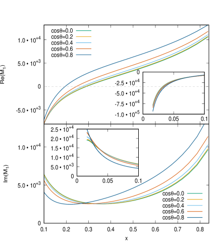
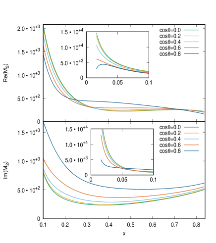
Figure 3: Behavior of ${\cal M}_{1}^{B,(2),fin}$ (left) and ${\cal M}_{2}^{B,(2),fin}$ (right) as a function of the scaling variable $x$ for different values of $\cos(\theta)$. The insets show the region close to $x=0$.

The finite remainders ${\cal M}_{i}^{B,(j),fin}$, $i=1,2$, computed in the previous section, are expressed in terms of multiple classical polylogarithms with arguments depending on the scaling variables $x,y$ and their coefficients further depending on the Higgs mass $m_{h}$. Since the analytical results are too long to be presented in this article, we have provided ancillary files containing the analytical results (and their numerical evaluation) in Mathematica format. In order to demonstrate the dependence of the two-loop finite remainders on the scaling variables $x$ and $y$ for $m_{h}=125$ GeV and with $\mu_{R}^{2}=m_{h}^{2}/2$, we plot real and imaginary parts of both ${\cal M}_{i}^{B,(2),fin}$, $i=1,2$ as a function of the partonic invariant mass variable $x$ for different choices of $\cos(\theta)$, where $\theta$ is the angle between one of the Higgs bosons in the final state and one of the initial gluons in their center of mass frame. We extract an additional factor of $m_{h}^{2}$ in the plots. The amplitude is invariant under $\cos(\theta)\to-\cos(\theta)$, as expected for a purely bosonic amplitude. Since this symmetry has not been used in the setup of the calculation, it serves as a strong check on our results.

In Fig. 3, we display the real and imaginary parts of the amplitude ${\cal M}_{1}^{B,(2),fin}$ (left panel) and ${\cal M}_{2}^{B,(2),fin}$ (right panel). The behavior of the amplitudes close to the production threshold, $x=0$, is shown in the insets. We see that the finite parts of the two-loop amplitude shows stable behavior, and they display a non-trivial dependence on the process kinematics.

In the numerical evaluations, the large rational coefficients of the classical polylogarithms can introduce numerical instabilities in case we do not demand high enough precision. In particular, there are large cancellations between the numerator and denominator of rational functions. Therefore, we evaluate the polylogarithms at double, and the rational coefficients at even higher precision.

5 Discussion and Conclusions

The two-loop massless corrections to the $g+g\to H+H$ amplitude derived above complete the set of purely virtual amplitudes required for the prediction of the N³LO corrections to Higgs boson pair production in gluon fusion, in the infinite top quark mass limit. All other amplitudes relevant at this order are either (class-A) known already from the calculation of inclusive gluon fusion Higgs boson production at N³LO Anastasiou:2015ema ; Mistlberger:2018etf or (class-B) amount to one-loop and tree-level amplitudes that can be computed using automated tools. The combination of these amplitudes into a fully differential N³LO calculation of Higgs boson pair production does still require substantial advances in the techniques for handling infrared singular real radiation configurations at this order, with first steps being taken most recently Currie:2018fgr ; Cieri:2018oms .

More imminent applications of the newly derived results to Higgs boson pair production are the computation of fixed order soft-virtual corrections to the total cross section or of the hard matching coefficients in the resummation of corrections at low pair transverse momentum.

In this paper, we have computed all virtual amplitudes that contribute to the production of a pair of Higgs bosons from the gluon-gluon initiated partonic processes at order $a_{s}^{4}$. The calculation is performed in an effective field theory where the top quark is integrated out, and all other quarks are massless. The exact calculation of top quark mass effects is currently out of reach at this order, but reweighting procedures allow to reliably quantify these effects Grazzini:2018bsd . We deal with two classes of amplitudes separately, named class-A (one effective operator insertion) and class-B (two effective operator insertions). The amplitudes of class-A can be related to the gluon form factor which is already known up to three loop order while amplitudes of class-B were known previously up to one loop. Our explicit computation of the two-loop corrections to the class-B amplitudes now completes the perturbative expansion of the $g+g\to H+H$ amplitude to order $a_{s}^{4}$. We observe that the pole structure of the amplitude is in agreement with predictions from infrared factorization, and provide (as ancillary files with the arXiv submission of this article) a numerical code to evaluate its finite remainder piece. The newly derived amplitudes open up opportunities for a new level of precision phenomenology predictions in Higgs boson pair production.

References

- (1) ATLAS collaboration, G. Aad et al., Observation of a new particle in the search for the Standard Model Higgs boson with the ATLAS detector at the LHC, Phys. Lett. B716 (2012) 1–29, [1207.7214].
- (2) CMS collaboration, S. Chatrchyan et al., Observation of a new boson at a mass of 125 GeV with the CMS experiment at the LHC, Phys. Lett. B716 (2012) 30–61, [1207.7235].
- (3) C. Englert, A. Freitas, M. M. Mühlleitner, T. Plehn, M. Rauch, M. Spira and K. Walz, Precision Measurements of Higgs Couplings: Implications for New Physics Scales, J. Phys. G41 (2014) 113001, [1403.7191].
- (4) S. Dawson, S. Dittmaier and M. Spira, Neutral Higgs boson pair production at hadron colliders: QCD corrections, Phys. Rev. D58 (1998) 115012, [hep-ph/9805244].
- (5) A. Djouadi, W. Kilian, M. Mühlleitner and P. M. Zerwas, Testing Higgs selfcouplings at linear colliders, Eur. Phys. J. C10 (1999) 27–43, [hep-ph/9903229].
- (6) A. Djouadi, W. Kilian, M. Mühlleitner and P. M. Zerwas, Production of neutral Higgs boson pairs at LHC, Eur. Phys. J. C10 (1999) 45–49, [hep-ph/9904287].
- (7) M. M. Mühlleitner, Higgs particles in the standard model and supersymmetric theories, Ph.D. thesis, Hamburg U., 2000. hep-ph/0008127.
- (8) E. W. N. Glover and J. J. van der Bij, Higgs boson pair production via gluon fusion, Nucl. Phys. B309 (1988) 282–294.
- (9) T. Plehn, M. Spira and P. M. Zerwas, Pair production of neutral Higgs particles in gluon-gluon collisions, Nucl. Phys. B479 (1996) 46–64, [hep-ph/9603205].
- (10) J. Baglio, A. Djouadi, R. Gröber, M. M. Mühlleitner, J. Quevillon and M. Spira, The measurement of the Higgs self-coupling at the LHC: theoretical status, JHEP 04 (2013) 151, [1212.5581].
- (11) V. Barger, L. L. Everett, C. B. Jackson and G. Shaughnessy, Higgs-Pair Production and Measurement of the Triscalar Coupling at LHC(8,14), Phys. Lett. B728 (2014) 433–436, [1311.2931].
- (12) M. J. Dolan, C. Englert and M. Spannowsky, Higgs self-coupling measurements at the LHC, JHEP 10 (2012) 112, [1206.5001].
- (13) A. Papaefstathiou, L. L. Yang and J. Zurita, Higgs boson pair production at the LHC in the channel, Phys. Rev. D87 (2013) 011301, [1209.1489].
- (14) D. E. Ferreira de Lima, A. Papaefstathiou and M. Spannowsky, Standard model Higgs boson pair production in the ()() final state, JHEP 08 (2014) 030, [1404.7139].
- (15) J. K. Behr, D. Bortoletto, J. A. Frost, N. P. Hartland, C. Issever and J. Rojo, Boosting Higgs pair production in the final state with multivariate techniques, Eur. Phys. J. C76 (2016) 386, [1512.08928].
- (16) R. Gröber, M. Mühlleitner and M. Spira, Higgs Pair Production at NLO QCD for CP-violating Higgs Sectors, Nucl. Phys. B925 (2017) 1–27, [1705.05314].
- (17) J. Grigo, J. Hoff, K. Melnikov and M. Steinhauser, On the Higgs boson pair production at the LHC, Nucl. Phys. B875 (2013) 1–17, [1305.7340].
- (18) R. Frederix, S. Frixione, V. Hirschi, F. Maltoni, O. Mattelaer, P. Torrielli, E. Vryonidou and M. Zaro, Higgs pair production at the LHC with NLO and parton-shower effects, Phys. Lett. B732 (2014) 142–149, [1401.7340].
- (19) F. Maltoni, E. Vryonidou and M. Zaro, Top-quark mass effects in double and triple Higgs production in gluon-gluon fusion at NLO, JHEP 11 (2014) 079, [1408.6542].
- (20) G. Degrassi, P. P. Giardino and R. Gröber, On the two-loop virtual QCD corrections to Higgs boson pair production in the Standard Model, Eur. Phys. J. C76 (2016) 411, [1603.00385].
- (21) R. Gröber, A. Maier and T. Rauh, Reconstruction of top-quark mass effects in Higgs pair production and other gluon-fusion processes, JHEP 03 (2018) 020, [1709.07799].
- (22) R. Bonciani, G. Degrassi, P. P. Giardino and R. Gröber, Analytical Method for Next-to-Leading-Order QCD Corrections to Double-Higgs Production, Phys. Rev. Lett. 121 (2018) 162003, [1806.11564].
- (23) S. Borowka, N. Greiner, G. Heinrich, S. Jones, M. Kerner, J. Schlenk, U. Schubert and T. Zirke, Higgs Boson Pair Production in Gluon Fusion at Next-to-Leading Order with Full Top-Quark Mass Dependence, Phys. Rev. Lett. 117 (2016) 012001, [1604.06447].
- (24) S. Borowka, N. Greiner, G. Heinrich, S. P. Jones, M. Kerner, J. Schlenk and T. Zirke, Full top quark mass dependence in Higgs boson pair production at NLO, JHEP 10 (2016) 107, [1608.04798].
- (25) D. de Florian and J. Mazzitelli, Two-loop virtual corrections to Higgs pair production, Phys. Lett. B724 (2013) 306–309, [1305.5206].
- (26) J. Grigo, J. Hoff and M. Steinhauser, Higgs boson pair production: top quark mass effects at NLO and NNLO, Nucl. Phys. B900 (2015) 412–430, [1508.00909].
- (27) D. de Florian and J. Mazzitelli, Higgs Boson Pair Production at Next-to-Next-to-Leading Order in QCD, Phys. Rev. Lett. 111 (2013) 201801,
- (28) J. Grigo, K. Melnikov and M. Steinhauser, Virtual corrections to Higgs boson pair production in the large top quark mass limit, Nucl. Phys. B888 (2014) 17–29, [1408.2422].
- (29) Q. Li, Q.-S. Yan and X. Zhao, Higgs Pair Production: Improved Description by Matrix Element Matching, Phys. Rev. D89 (2014) 033015, [1312.3830].
- (30) P. Maierhöfer and A. Papaefstathiou, Higgs Boson pair production merged to one jet, JHEP 03 (2014) 126, [1401.0007].
- (31) D. de Florian and J. Mazzitelli, Higgs pair production at next-to-next-to-leading logarithmic accuracy at the LHC, JHEP 09 (2015) 053, [1505.07122].
- (32) M. Grazzini, G. Heinrich, S. Jones, S. Kallweit, M. Kerner, J. M. Lindert and J. Mazzitelli, Higgs boson pair production at NNLO with top quark mass effects, JHEP 05 (2018) 059, [1803.02463].
- (33) D. Y. Shao, C. S. Li, H. T. Li and J. Wang, Threshold resummation effects in Higgs boson pair production at the LHC, JHEP 07 (2013) 169, [1301.1245].
- (34) A. Djouadi, M. Spira and P. M. Zerwas, Production of Higgs bosons in proton colliders: QCD corrections, Phys. Lett. B264 (1991) 440–446.
- (35) M. Kramer, E. Laenen and M. Spira, Soft gluon radiation in Higgs boson production at the LHC, Nucl. Phys. B511 (1998) 523–549, [hep-ph/9611272].
- (36) K. G. Chetyrkin, B. A. Kniehl and M. Steinhauser, Hadronic Higgs decay to order , Phys. Rev. Lett. 79 (1997) 353–356, [hep-ph/9705240].
- (37) M. Spira, Effective Multi-Higgs Couplings to Gluons, JHEP 10 (2016) 026, [1607.05548].
- (38) M. Gerlach, F. Herren and M. Steinhauser, Wilson coefficients for Higgs boson production and decoupling relations to , 1809.06787.
- (39) P. A. Baikov, K. G. Chetyrkin, A. V. Smirnov, V. A. Smirnov and M. Steinhauser, Quark and gluon form factors to three loops, Phys. Rev. Lett. 102 (2009) 212002, [0902.3519].
- (40) T. Gehrmann, E. W. N. Glover, T. Huber, N. Ikizlerli and C. Studerus, Calculation of the quark and gluon form factors to three loops in QCD, JHEP 06 (2010) 094, [1004.3653].
- (41) M. F. Zoller, On the renormalization of operator products: the scalar gluonic case, JHEP 04 (2016) 165, [1601.08094].
- (42) N. K. Nielsen, Gauge Invariance and Broken Conformal Symmetry, Nucl. Phys. B97 (1975) 527–540.
- (43) V. P. Spiridonov and K. G. Chetyrkin, Nonleading mass corrections and renormalization of the operators and , Sov. J. Nucl. Phys. 47 (1988) 522–527.
- (44) A. L. Kataev, N. V. Krasnikov and A. A. Pivovarov, Two Loop Calculations for the Propagators of Gluonic Currents, Nucl. Phys. B198 (1982) 508–518, [hep-ph/9612326].
- (45) S. Catani, The Singular behavior of QCD amplitudes at two loop order, Phys. Lett. B427 (1998) 161–171, [hep-ph/9802439].
- (46) G. F. Sterman and M. E. Tejeda-Yeomans, Multiloop amplitudes and resummation, Phys. Lett. B552 (2003) 48–56, [hep-ph/0210130].
- (47) T. Becher and M. Neubert, Infrared singularities of scattering amplitudes in perturbative QCD, Phys. Rev. Lett. 102 (2009) 162001, [0901.0722].
- (48) E. Gardi and L. Magnea, Factorization constraints for soft anomalous dimensions in QCD scattering amplitudes, JHEP 03 (2009) 079, [0901.1091].
- (49) P. Nogueira, Automatic Feynman graph generation, J. Comput. Phys. 105 (1993) 279–289.
- (50) J. A. M. Vermaseren, New features of FORM, math-ph/0010025.
- (51) A. von Manteuffel and C. Studerus, Reduze 2 - Distributed Feynman Integral Reduction, 1201.4330.
- (52) T. Gehrmann, A. von Manteuffel, L. Tancredi and E. Weihs, The two-loop master integrals for , JHEP 06 (2014) 032, [1404.4853].
- (53) F. Cascioli, T. Gehrmann, M. Grazzini, S. Kallweit, P. Maierhöfer, A. von Manteuffel, S. Pozzorini, D. Rathlev, L. Tancredi and E. Weihs, ZZ production at hadron colliders in NNLO QCD, Phys. Lett. B735 (2014) 311–313, [1405.2219].
- (54) T. Gehrmann, M. Grazzini, S. Kallweit, P. Maierhöfer, A. von Manteuffel, S. Pozzorini, D. Rathlev and L. Tancredi, Production at Hadron Colliders in Next to Next to Leading Order QCD, Phys. Rev. Lett. 113 (2014) 212001, [1408.5243].
- (55) F. Caola, J. M. Henn, K. Melnikov, A. V. Smirnov and V. A. Smirnov, Two-loop helicity amplitudes for the production of two off-shell electroweak bosons in quark-antiquark collisions, JHEP 11 (2014) 041, [1408.6409].
- (56) T. Gehrmann, A. von Manteuffel and L. Tancredi, The two-loop helicity amplitudes for leptons, JHEP 09 (2015) 128, [1503.04812].
- (57) A. von Manteuffel and L. Tancredi, The two-loop helicity amplitudes for , JHEP 06 (2015) 197, [1503.08835].
- (58) F. Caola, J. M. Henn, K. Melnikov, A. V. Smirnov and V. A. Smirnov, Two-loop helicity amplitudes for the production of two off-shell electroweak bosons in gluon fusion, JHEP 06 (2015) 129, [1503.08759].
- (59) F. V. Tkachov, A Theorem on Analytical Calculability of Four Loop Renormalization Group Functions, Phys. Lett. 100B (1981) 65–68.
- (60) K. G. Chetyrkin and F. V. Tkachov, Integration by Parts: The Algorithm to Calculate beta Functions in 4 Loops, Nucl. Phys. B192 (1981) 159–204.
- (61) T. Gehrmann and E. Remiddi, Differential equations for two loop four point functions, Nucl. Phys. B580 (2000) 485–518, [hep-ph/9912329].
- (62) S. Laporta, High precision calculation of multiloop Feynman integrals by difference equations, Int. J. Mod. Phys. A15 (2000) 5087–5159, [hep-ph/0102033].
- (63) C. Anastasiou and A. Lazopoulos, Automatic integral reduction for higher order perturbative calculations, JHEP 07 (2004) 046, [hep-ph/0404258].
- (64) A. V. Smirnov, Algorithm FIRE – Feynman Integral REduction, JHEP 10 (2008) 107, [0807.3243].
- (65) C. Studerus, Reduze-Feynman Integral Reduction in C++, Comput. Phys. Commun. 181 (2010) 1293–1300, [0912.2546].
- (66) R. N. Lee, LiteRed 1.4: a powerful tool for reduction of multiloop integrals, J. Phys. Conf. Ser. 523 (2014) 012059, [1310.1145].
- (67) T. Gehrmann, L. Tancredi and E. Weihs, Two-loop master integrals for : the planar topologies, JHEP 08 (2013) 070, [1306.6344].
- (68) C. Anastasiou, C. Duhr, F. Dulat, F. Herzog and B. Mistlberger, Higgs Boson Gluon-Fusion Production in QCD at Three Loops, Phys. Rev. Lett. 114 (2015) 212001, [1503.06056].
- (69) B. Mistlberger, Higgs boson production at hadron colliders at N3LO in QCD, JHEP 05 (2018) 028, [1802.00833].
- (70) J. Currie, T. Gehrmann, E. W. N. Glover, A. Huss, J. Niehues and A. Vogt, N3LO corrections to jet production in deep inelastic scattering using the Projection-to-Born method, JHEP 05 (2018) 209, [1803.09973].
- (71) L. Cieri, X. Chen, T. Gehrmann, E. W. N. Glover and A. Huss, Higgs boson production at the LHC using the subtraction formalism at N3LO QCD, [1807.11501].