Do we live in an eigenstate of the “fundamental constants” operators?

Abstract

We propose that the constants of Nature we observe (which appear as parameters in the classical action) are quantum observables in a kinematical Hilbert space. When all of these observables commute, our proposal differs little from the treatment given to classical parameters in quantum information theory, at least if we were to inhabit a constants’ eigenstate. Non-commutativity introduces novelties, due to its associated uncertainty and complementarity principles, and it may even preclude hamiltonian evolution. The system typically evolves as a quantum superposition of hamiltonian evolutions resulting from a diagonalization process, and these are usually quite distinct from the original one (defined in terms of the non-commuting constants). We present several examples targeting $G$, $c$ and $\Lambda$, and the dynamics of homogeneous and isotropic Universes. If we base our construction on the Heisenberg algebra and the quantum harmonic oscillator, the alternative dynamics tends to silence matter (effectively setting $G$ to zero), and make curvature and the cosmological constant act as if their signs are reversed. Thus, the early Universe expands as a quantum superposition of different Milne or de Sitter expansions for all material equations of state, even though matter nominally dominates the density, $\rho$, because of the negligible influence of $G\rho$ on the dynamics. A superposition of Einstein static universes can also be obtained. We also investigate the results of basing our construction on the algebra of $SU(2)$, into which we insert information about the sign of a constant of Nature, or whether its action is switched on or off. In this case we find examples displaying quantum superpositions of bounces at the initial state for the Universe.

I Introduction

It is sombering to recognise that we have never successfully predicted the values of any fundamental dimensionless constants of Nature, yet we measure them with our most accurate experiments: they combine our greatest experimental knowledge with our greatest theoretical ignorance. Historically, there have been different attitudes and expectations regarding the numerical values of the constants of Nature. Einstein ein believed there was a single logically self-consistent, rigid, theory of everything (a “unified field theory”) whose defining constants were uniquely and completely specified. The direction of modern particle physics and cosmology now prefers the opposite view that there are many self-consistent theories of everything, with different suites of defining constants of Nature, and we inhabit one of them as a result of random symmetry-breakings at ultra-high energies. The question of how much of our known low-energy physics must necessarily reside in the vacuum state of one of these many possible theories of everything remains open swamp .

These scenarios open up the possibility that the low-energy constants of physics could be different – and may even be different in widely separated places in the universe on both sub and super-horizon scales. An added complexion arises from the prospect that the quantities we call constants of Nature may not be the fundamental unchanging constants defining the most basic theory of everything. Our observed “constants” may therefore be allowed to be time and/or space dependent variables jdb2 without undermining the invariant status of the true constants in the most basic theory. A simple example is provided by 3-d constants in a 3-d submanifold of a higher-dimensional theory in which any time change in the mean size of additional dimensions will be seen in the time change of the 3-d “constants” 3d , like the fine structure constant and its effects on quasar spectra at high redshifts webb .

We note that all previous attempts to variabilize the constants of Nature have been classical: one produces an action principle for which one or more constants (e.g. the particles masses, the coupling constants, and $G$, $c$ or even $\hbar$) are promoted to dynamical (scalar) fields BD ; B ; SBM . Any quantization of these fields is banned. In this paper we speculate further that the set up of “varying constants” may be purely quantum and devoid of a classical counterpart. In such a situation the constants that we observe would have fixed values but they would not need to be unique. That is the speculative avenue to be explored in this paper.

Usually we start from a classical system (or theory), and then “quantize” via a given prescription, such as canonical quantization or the path integral formalism. The possible pitfalls are well-known. The quantum theory contains more information than the classical theory, so ambiguities arise, such as ordering issues, inner product uncertainties, or a multitude of options for the quantum implementation of constraints, should they exist. Quite often a given classical system or theory leads to a variety of quantum analogues, no matter how careful the quantization procedure is, and we know of no way to generate quantum solutions of a theory directly from solutions of its classical counterpart.

Another example of the conceptual difficulties plaguing the interaction between the classical and quantum worlds is found in the opposite direction, when one seeks a classical or semi-classical limit of quantum theories. Quantum gravity has been a major source of trouble in this respect, with mathematically consistent non-perturbative constructions risking being nothing but a figment of our imagination for want of a suitable (semi-) classical limit. Even in more mundane situations (and ignoring the notorious measurement problem) one can say that the quantum and classical worlds sit together rather uneasily. But could it be that in some situations, such as near the start of our universe, this interaction happens in a totally novel way? In this paper we propose that the constants of Nature are quantum observables in a purely kinematic Hilbert space, and that we are currently living in an eigenstate of their corresponding operators. An eigenstate corresponds to a classical lagrangian with fixed constants and a dynamics which may then be quantized by traditional methods. We present the formalism in Section II, allowing for superpositions of such dynamics.

The non-trivial aspects of this proposal start when we elaborate this basic picture: for example, by allowing two constants to be non-commuting observables (Section III). Then, a fundamental indeterminacy would even be built into the classical dynamics. In fact complementarity may preclude hamiltonian evolution altogether. We illustrate these points with a toy model in Section IV: a simple harmonic oscillator for which the mass and the spring constant are non-commuting constant observables. Depending on technical assumption, a diagonalization procedure may be possible, leading to alternative dynamics. The general evolution of the system is then a quantum superposition of these qualitatively different evolutions.

For the rest of the paper we transpose this construction to cosmology, targeting $G$, $c$ and $\Lambda$, and the dynamics of homogeneous and isotropic Universes. In Sections V, VI and VII we examine what happens if $G$ and $c$ are complementary variables. We find that, even though matter dominates the spatial curvature $K$ and $\Lambda$ early on, it does not affect the expansion of the Universe, which can be a general superposition of Milne (if $K=1$ and $\Lambda=0$) or de Sitter (if $K=0$ and $\Lambda<0$) expansion profiles. In general the universe evolves as a quantum superposition of dynamics ruled by effectively setting $G$ to zero, quantizing the speed of light, and reversing the effective signs of $K$ and $\Lambda$. A similar pattern can be obtained by making $c$ and $\Lambda$ a complementary pair (Section VII.2). Superpositions of stable static universes also appear as solutions (Section VII.3).

Instead, in Section VIII and IX we base our construction on the algebra of $SU(2)$, into which we insert information about the sign of $G$, $\Lambda$ and $K$, or whether their action is switched on or off. We find examples displaying quantum superpositions of bounces at the initial state for the Universe.

Finally, in two concluding Sections we discuss the physical meaning of our construction, summarise its main results and outline some of its open problems,

II The simplest model

Let us consider a classical dynamics defined by an action, $S$, which is a functional over generic variables (or fields) globally denoted by $x$, and that depends on $n$ “constants”, $\kappa_{i}$:

$$S=\int\mathcal{L}(x;\kappa_{i}).$$ (1)

The associated hamiltonian (obtained while keeping $\kappa_{i}$ constant) is:

$$\mathcal{H}=\mathcal{H}(x,p;\kappa_{i})=\mathcal{L}-pq,$$ (2)

with $x$ and conjugate momenta $p$ satisfying a diagonal Poisson bracket:

$$\{x,p\}=\delta,$$ (3)

(where the Dirac/Kronecker $\delta$ involves all indices and variables on which the $x$ and $p$ depend). First, we construct a Hilbert space $\mathbb{H}$ in which the $\kappa_{i}$ are represented by Hermitian operators, $\hat{\kappa}_{i}$ (“observables”), with eigenstates associated with eigenvalues $\kappa_{i}$ for the constants:

$$\hat{\kappa}_{i}|\kappa_{i}\rangle=\kappa_{i}|\kappa_{i}\rangle.$$ (4)

Since this is a theory of these “constants”, no dynamics (or quantum hamiltonian) is given to Hilbert space $\mathbb{H}$, i.e. it is a purely kinematical Hilbert space. This is the first non-conventional assumption of our proposal.

Next, we first assume that the various constants, $\kappa_{i}$, commute with each other, so that their operators can be diagonalized simultaneously. Then, there is an orthogonal basis of eigenvectors for all the $\hat{\kappa}_{i}$, satisfying:

$$\langle\kappa_{1}^{\prime}...\kappa_{n}^{\prime}|\kappa_{1}...\kappa_{n}\rangle=\prod_{i=1}^{n}\delta(\kappa_{i}^{\prime}-\kappa_{i}).$$ (5)

We propose that being in an eigenstate of the $\hat{\kappa}_{i}$ entails not only the observation of the values of the constants $\kappa_{i}$ corresponding to their eigenvalues, but also of the classical dynamics defined by $\mathcal{H}(x,p;\kappa_{i})$ on the base space defined by $x,p$ and endowed with a Poisson bracket. This system is never classical overall; however, there is classical behaviour, if we are in the eigenstate. Note that the constants are not “varying” in time or space, they can just be observed to on take different values: each quantum outcome has different fixed constants. We might think of this picture as a Hilbert space of theories. As long as we stick to eigenstates we have a variation on the theme of the “multiverse” multi , perhaps with a more quantum flavour, but not substantially different in its implications.

We can ask what happens to the classical dynamics encoded in $\mathcal{H}(x,p;\kappa_{i})$ should we have a superposition of the $|\kappa_{i}\rangle$? We postulate that we would then have a superposition of classical phase spaces, each endowed with a different hamiltonian labelled by the $\kappa_{i}$. That is, we would have a superposition of all the solutions mapped from the initial conditions by the different evolutions. This proposal has a definite flavour of the many-worlds interpretation of quantum mechanics, but applied to the full set of classical solutions and dynamics.

We represent the total hamiltonian of the system by

$$\hat{\mathcal{H}}_{tot}(x,p)=\int d^{n}\kappa_{i}\,|\kappa_{i}\rangle\langle\kappa_{i}|\otimes\mathcal{H}(x,p;\kappa_{i}).$$ (6)

Here, the $\mathcal{H}(x;\kappa_{i})$ are (at least initially) classical, and the Poisson bracket structure only applies to them. The $\hat{\mathcal{H}}_{tot}|\Psi\rangle$ represents the postulated superposition for the state $|\Psi\rangle\in\mathcal{H}$. The symbol $\otimes$ could represent the usual bilinear tensor product or any other structure, possibly more complex. Some notational simplification can be obtained by defining a composite object

$$x_{\Psi}(t)=|\Psi\rangle\otimes x=\int d\kappa_{i}\,\Psi(\kappa_{i})|\kappa_{i}\rangle\otimes x(t;\kappa_{i}),$$ (7)

representing the superposition of hamiltonian evolutions for the various parameters $\kappa_{i}$, with amplitudes determined by the wavefunction:

$$|\Psi\rangle=\int d\kappa_{i}\Psi(\kappa_{i})|\kappa_{i}\rangle.$$ (8)

Then, we can define

$$\dot{x}_{\Psi} = \{x_{\Psi},\hat{\mathcal{H}}_{tot}\},$$ (9)

$$\dot{p}_{\Psi} = \{p_{\Psi},\hat{\mathcal{H}}_{tot}\},$$ (10)

as long as we assume that, by definition, all the quantum quantities to the left of $\otimes$ act only on themselves as appropriate, and the Poisson bracket only involves the classical quantities on the right of $\otimes$. Indeed, the left-hand side of (9) can then be written as:

$$\{|\Psi\rangle\otimes x,\hat{\mathcal{H}}_{tot}\} = \int d\kappa_{i}|\kappa_{i}\rangle\langle\kappa_{i}|\Psi\rangle\otimes\{x,\mathcal{H}(x,p;\kappa_{i})\}$$ (11)

$$= \int d\kappa_{i}\Psi(\kappa_{i})|\kappa_{i}\rangle\otimes\dot{x}(t;\kappa_{i})$$

$$= |\Psi\rangle\otimes\dot{x}=\dot{x}_{\Psi},$$

and likewise, for (10).

As long as we live in an eigenstate of the constants’ operator (which assumes they commute), the proposal in this Section is very similar to the treatment given to classical parameters in quantum information theory Qinf , where they are elevated to bras and kets with the property (5). The total hamiltonian is then written as (6), except that in quantum information theory the $\mathcal{H}(x,p;\kappa_{i})\equiv\hat{\mathcal{H}}(\hat{x},\hat{p};\kappa_{i})$ already is a quantum hamiltonian operator. Thus, at this stage, our proposal is quite standard, as long as the $\Psi$ are eigenstates. Inevitable novelties arise though if we now move on to assume that the $\hat{\kappa}_{i}$ do not commute.

III Non-commuting constants

Our model becomes significantly different if some of the constants do not commute. In general, they might form an algebra:

$$[\hat{\kappa}_{i},\kappa_{j}]=if_{ijk}\hat{\kappa}_{k},$$ (12)

and later we will consider examples targeting particular “constants”, for example, $\hat{G}$, $\hat{c}$ and $\hat{\Lambda}$. This would introduce a fundamental indeterminacy in their value, according to the Heisenberg Uncertainty Principle. First consider the situation in which just two constants are conjugates:

$$\left[\hat{\kappa}_{1},\hat{\kappa}_{2}\right]=i\mathfrak{h}$$ (13)

where $\mathfrak{h}$ is a possibly dimensionful constant (the dimensions will depend on the model), which may or may not be proportional to the usual Planck constant. As is well known, following a purely kinematical argument, we must have:

$$\Delta^{2}\kappa_{1}\Delta^{2}\kappa_{2}\geq\frac{\mathfrak{h}^{2}}{4}.$$ (14)

One might therefore think that the evolution would take place in the form of a “fuzzy” hamiltonian evolution in which the parameters are undetermined, at least if the $|\Psi\rangle$ wavefunction is taken to be a coherent state.

However, this is not the case. It turns out that the evolution is qualitatively different, and in fact there may not be any form of conventional hamiltonian evolution at all. The key point is that we now have a complementarity principle in operation: asking the system about the value of one constant precludes asking questions about the other. Although it is true that an eigenstate of, say, $\hat{\kappa}_{1}$ can be written as a superposition of eigenstates of $\hat{\kappa}_{2}$, this superposition does not represent a superposition of the simultaneous observation of the original eigenvalue $\kappa_{1}$ and each of the eigenvalues of $\hat{\kappa}_{2}$. This is a trivial point, but it should be stressed. Therefore, not only can we never be in an eigenstate of all the constants, but we can also never be in a superposition of states with a well defined hamiltonian in terms of the original constants. In terms of the original hamiltonian, there can never be any hamiltonian evolution for the system, or even a superposition thereof, because we cannot muster enough information to define the classical hamiltonian, or even a superposition as envisaged in Section II.

In other words, the replacement

$$\mathcal{H}(x,p;\kappa_{1},\kappa_{2})\rightarrow\mathcal{H}_{tot}(x,p;\hat{\kappa}_{1},\hat{\kappa}_{2})$$ (15)

may be done, but this can never be unravelled in the format (6), resulting in a superposition of classical hamiltonian evolutions defined by $\mathcal{H}(x,p;\kappa_{1},\kappa_{2})$. At best, we might be able to obtain, for example, something like:

$$\hat{\mathcal{H}}_{tot}(x,p) = \int d\kappa_{1}\,|\kappa_{1}\rangle\langle\kappa_{1}|\otimes\mathcal{H}_{1}(x,p;\kappa_{1})$$

$$+ \int d\kappa_{2}\,|\kappa_{2}\rangle\langle\kappa_{2}|\otimes\mathcal{H}_{2}(x,p;\kappa_{2}),$$

if the classical (“proto”) hamiltonian can be split as

$$\mathcal{H}(x,p;\kappa_{1},\kappa_{2})=\mathcal{H}_{1}(x,p;\kappa_{1})+\mathcal{H}_{2}(x,p;\kappa_{2}).$$ (16)

The lack of straightforward hamiltonian evolution would then be signalled by the time derivatives of the states $x_{\Psi}$ and $p_{\Psi}$ not equalling states in the original $|\Psi\rangle$ (cf. eqns. (9) and (10)).

This does not mean that nothing can be said about the evolution of the system, as we will show in the following Sections. The technical inputs of the theory are

• The structure of the Hilbert space $\mathbb{H}$: its inner product, and kinematic observables $\hat{\kappa}_{i}$).

• The state $|\Psi\rangle\in\mathbb{H}$ in which we live.

• The algebra of commutators (12).

• The combined hamiltonian $\mathcal{H}_{tot}$ and its $\otimes$ structure.

Note that the $\otimes$ encodes how the quantum constants interact with the classical hamiltonian. This can be non-linear and as complex as wanted. Depending on the inputs above (point d in particular) we could conceivably find that hamiltonian dynamics is impossible. However, it may also be preserved in some form.

To clarify and summarise the proposal made in the last two sections: we have elevated the constants of Nature to quantum operators, but these live in a purely quantum kinematical Hilbert space. They do not have classical counterparts, and their commutator does not result from a classical Poisson bracket (although this could be explored and is left for future work; see quantumlambda for an instance of this approach regarding the quantum cosmological constant). Concomitantly, the commutators of these constants do not generate any time evolution for them: in this sense they are the genuine constants.

Note also the difference with notime , where the existence of a dynamical hamiltonian for the constants is precluded by the fact that localized time disintegrates, so that a hamiltonian structure is not possible. Here, the kinematical nature of the constants’ Hilbert space is a choice, and it does blend in with a hamiltonian structure for $x$ and $p$. The fact that the constants may not commute precludes in general the existence of a hamiltonian evolution, at least in terms of the original hamiltonian, since no state can summon enough information to specify the hamiltonian. In some cases, a counterpart to a hamiltonian evolution can be found, as we shall now see .

IV An illustrative toy model

We will now apply our formalism to a metaphorical toy model – not to be taken literally as a physical model. It is intended only to illustrate our proposal for the constants of Nature. Consider a harmonic oscillator with action:

$$S(x,\dot{x};m,k)=\int dt\left(\frac{p^{2}}{2m}-\frac{kx^{2}}{2}\right),$$ (17)

and hamiltonian:

$$\mathcal{H}(x,p;m,k)=\frac{p^{2}}{2m}+\frac{kx^{2}}{2}.$$ (18)

Here, the spring constant, $k$, and the mass, $m$, play the role of “constants” of Nature. The proposal in this paper is that $m$ and $k$ should be promoted to observables, $\hat{m}$ and $\hat{k}$, in an essentially kinematical Hilbert space, $\mathbb{H}$.

If these observables commute, and if we live in an eigenstate of the constants’ operator, the usual classical theory follows, with a treatment given to its parameters reminiscent of quantum information theory. We would then say that there are joint eigenstates $|k,m\rangle$ for which:

$$\langle k^{\prime}m^{\prime}|k,m\rangle=\delta(k-k^{\prime})\delta(m-m^{\prime}),$$ (19)

such that the total hamiltonian is given by

$$\hat{\mathcal{H}}_{tot}(x,p)=\int dm\,dk\,|k,m\rangle\langle km|\otimes\mathcal{H}(x,p;m,k).$$ (20)

If the system lives in an eigenstate $|k,m\rangle$ then the dynamics encoded in $\mathcal{H}(x,p;m,k)$ are observed. For a general superposition of states $|\Psi\rangle$, we postulate a superposition of all the possible dynamics and its solution $x_{\Psi}(t)$, with the amplitudes given by $\langle km|\Psi\rangle$.

Further quantum behaviour follows if $\hat{m}$ and $\hat{k}$ do not commute. Then, we can never be in an eigenstate of both constants and, as stated above, classical hamiltonian evolution in terms of the original hamiltonian is generally not possible. A replacement for a hamiltonian evolution (or a superposition thereof) might be found, however, depending on the assumptions of the theory, as we now exemplify.

One example where some sort of hamiltonian evolution survives is when the $\otimes$ product is a simple bilinear tensor product. Let us consider, furthermore, that:

$$\hat{\mathcal{H}}_{tot}=\hat{\kappa}_{2}^{2}\otimes\frac{p^{2}}{2}+\hat{\kappa}_{1}^{2}\otimes\frac{x^{2}}{2},$$ (21)

that is, we write operators $\hat{m}$ and $\hat{k}$ in terms of variables:

$$\hat{\kappa}_{1}^{2} = \widehat{\frac{1}{m}}$$ (22)

$$\hat{\kappa}_{2}^{2} = \hat{k}$$ (23)

with the assumption:

$$[\hat{\kappa}_{1},\hat{\kappa}_{2}]=i\mathfrak{h}$$ (24)

(in this example dimensions imply $[\mathfrak{h}]=1/T$). As explained before, $\hat{\mathcal{H}}$ is not to be seen as a hamiltonian for $\hat{\kappa}_{1}$ and $\hat{\kappa}_{2}$ (i.e., no Heisenberg equations for them are to be generated): their Hilbert space is kinematical. In contrast, $x$ and $p$ are classical dynamical variables, with Poisson bracket: $\{x,p\}=1$.

Although no hamiltonian evolution is possible in terms of the original constants, with such a simple $\otimes$ product we can diagonalize the hamiltonian in $\hat{\kappa}_{1}$ and $\hat{\kappa}_{2}$ by introducing the non-Hermitian operator $\hat{\alpha}$, such that:

$$\hat{\kappa}_{1}\otimes 1 = \frac{\hat{\alpha}+\hat{\alpha}^{\dagger}}{\sqrt{2}}\otimes\sqrt{\frac{\mathfrak{h}p}{x}}$$ (25)

$$\hat{\kappa}_{2}\otimes 1 = \frac{\hat{\alpha}-\hat{\alpha}^{\dagger}}{{\sqrt{2}}i}\otimes\sqrt{\frac{\mathfrak{h}x}{p}}.$$ (26)

Using the assumed bilinearity of $\otimes$ we can compute:

$$[\hat{\alpha},\hat{\alpha}^{\dagger}]=1$$ (27)

and:

$$\hat{\mathcal{H}}_{tot}=\frac{\hat{\alpha}\hat{\alpha}^{\dagger}+\hat{\alpha}^{\dagger}\hat{\alpha}}{2}\otimes\mathfrak{h}xp=\left(\hat{\alpha}^{\dagger}\hat{\alpha}+\frac{1}{2}\right)\otimes\mathfrak{h}xp.$$ (28)

We can therefore set up a Fock space representation for the Hilbert space where $\hat{\kappa}_{1}$ and $\hat{\kappa}_{2}$ live, i.e. in terms of the eigenstates $|n\rangle$ of $\hat{N}=\hat{\alpha}^{\dagger}\hat{\alpha}$. In this representation the total hamiltonian is given by:

$$\hat{\mathcal{H}}_{tot}=\sum_{n}|n\rangle\langle n|\otimes\mathfrak{h}\left(n+\frac{1}{2}\right)xp,$$ (29)

so it is diagonal.

We find two interesting results. Firstly, we see that, although there is no hamiltonian evolution in terms of the dynamics dependent on the original constants (here $\kappa_{1}$ and $\kappa_{2}$), the system does have a hamiltonian evolution in terms of another observable (here $\hat{N}$) quite different from the original constants. Since any state in the Hilbert space can be written as a superposition of the eigenstates of the new observable, the most general evolution corresponds to a superposition of the new hamiltonian evolutions. This includes the eigenstates of the original constants or any coherent state written in terms of them. In terms of the original constants, the evolution is therefore a quantum superposition of hamiltonian evolutions. For an eigenstate of $\hat{\kappa_{1}}$ or ($\hat{\kappa_{2}}$) the amplitudes $\langle n|\kappa_{1}\rangle$ would be the usual expressions in terms of Hermite polynomials. For a coherent state, defined from $\hat{\alpha}|\alpha\rangle=\alpha|\alpha\rangle,$ we would have instead:

$$\langle n|\alpha\rangle=e^{-\frac{|\alpha|^{2}}{2}}\frac{\alpha^{n}}{\sqrt{n!}}.$$ (30)

Secondly, we see that each of the hamiltonian evolutions that the system does admit is qualitatively different from the original one (possible only if the original constants were classical numbers, or commuting quantum operators and we selected one of their simultaneous eigenstates). Specifically, from (29), we see that each classical hamiltonian associated with $n$ is given by:

$$\mathcal{H}_{n}(x,p;n)=\mathfrak{h}\left(n+\frac{1}{2}\right)xp.$$ (31)

The dynamical equations are therefore:

$$\dot{x} = \mathfrak{h}\left(n+\frac{1}{2}\right)x$$ (32)

$$\dot{p} = -\mathfrak{h}\left(n+\frac{1}{2}\right)p$$ (33)

$$\dot{\mathcal{H}}_{n} = 0$$ (34)

with solutions:

$$x = C\exp{\left[\mathfrak{h}\left(n+\frac{1}{2}\right)t\right]}$$ (35)

$$p = C\exp{\left[-\mathfrak{h}\left(n+\frac{1}{2}\right)t\right]}.$$ (36)

Here $C$ is an integration constant related to the constant hamiltonian:

$$\mathcal{H}_{n}=C^{2}\left(n+\frac{1}{2}\right).$$ (37)

Closer examination shows that the qualitatively different dynamics can be traced to the selection of positive frequencies states $|n\rangle$. States with $n<0$ exist but are not normalizable. Excluding them demands $xp>0$, so clearly the dynamics in $x,p$ phase space had to be significantly modified (indeed by replacing the original harmonic oscillator by an inverted one with a quantized instability constant).

V Direct cosmological applications

The toy model of the preceding Section turns out to be formally very close to a real cosmological situation: a closed Friedmann universe filled with radiation, which has the dynamics of a simple harmonic oscillator. Indeed, we have the Friedmann equation for the metric scale factor $a(\tau)$, in conformal time $\tau$ with usual constant curvature parameter $K=0,$or $\pm 1$:

$$a^{\prime 2}+Kc^{2}a^{2}=\frac{8\pi G}{3}M,$$ (38)

where ^′ denotes a derivative with respect to $\tau$, so we have the simple oscillator in conformal time:

$$a^{\prime\prime}=-Kc^{2}a.$$

For a closed Friedmann radiation universe, we take

$$K = 1,$$ (39)

$$M = \rho a^{4}.$$ (40)

This can be easily transposed into the model in Section IV. Note that for our proposed constant quantization, it matters where we put the constants in the initial classical hamiltonian – as is often the case, equivalent classical theories may lead to different quantum theories. In particular, it is not indifferent for our procedure whether $G$ multiplies the matter density, or divides the Einstein-Hilbert (EH) action, even though this is equivalent classically. We will at first assume that the EH action is multiplied by $c^{2}/G$, rather than having $G/c^{2}$ multiplying the matter hamiltonian, before a transition to operators is imposed. With this choice the hamiltonian has units of mass density. Other choices will be explored later.

Specifically, let us assume a situation where we write the hamiltonian constraint implied by (38) as:

$$\mathcal{H}(a,p;G,c)=G\frac{p^{2}}{2}+\frac{c^{2}}{G}\frac{a^{2}}{2}\approx\frac{4\pi M}{3}$$ (41)

where $\approx$ means on-shell and $p=a^{\prime}/G$ is implied by the Hamilton equation:

$$a^{\prime}=\{a,H\}=Gp,$$ (42)

with the usual Poisson bracket $\{a,p\}=1$. We can subject this classical theory to our quantization of constants procedure, directly lifting results from the previous Section (cf. Eq.21), with the identifications:

$$\hat{\kappa}_{1}^{2} = \widehat{\frac{c^{2}}{G}},$$ (43)

$$\hat{\kappa}_{2}^{2} = \hat{G}.$$ (44)

Thus, $\hat{\kappa}_{2}=\sqrt{\hat{G}}$ and $\kappa_{1}$ can be any linear combination of $\hat{c}(\hat{G})^{-1/2}$ and $(\hat{G})^{-1/2}\hat{c}$, and we can check that

$$[\hat{c},\hat{G}]=2i\mathfrak{h}\hat{G}$$ (45)

enforces the required (24). Concomitant with the hamiltonian having units of a mass density, in this example, the quantity $\mathfrak{h}$ (playing the role of a dimensionally corrected Planck’s constant of unknown numerical value) has units of a speed.

We can therefore use the results of the previous Section to conclude that the most general solution for the Friedmann metric scale factor is a superposition of solutions of the form

$$a=C\exp{\left[\mathfrak{h}\left(n+\frac{1}{2}\right)\eta\right],}$$ (46)

with $n$ labelling the terms of the diagonalized hamiltonian (29), and producing a discretized Hubble expansion rate. This is a superposition of Milne universes, since they are exponential in conformal time, not proper time, $t$, where $dt=ad\tau$. However, the dynamics behind it is very different from that of the general relativistic Milne universe (for example, we have $K=+1$, rather than $K=-1$). Note, for example, that the $a$ evolution can be obtained without $p$. We find for $p$, independently, that

$$p=\frac{4\pi}{3}\frac{\rho a^{3}}{\mathfrak{h}(n+\frac{1}{2})},$$ (47)

either directly from $\mathcal{H}_{n}\approx\frac{4\pi M}{3}$, or from the Hamilton equation for $p$.

VI More general equations of state

The previous result is very robust. It is valid regardless of the matter equation of state. This can be checked via the transformation to $y(\tau)$ mentioned above. We present an alternative method at the end of this Section, to which we refer the reader who wishes to skip the mathematics details. It can also be checked that the same result is obtained using either conformal or proper time, dispelling obvious breaking of Lorentz invariance. We start by explaining how to do more general calculations, deriving a general rule of thumb.

Note first that the algebraic manipulations leading to (29) do not rely on the hamiltonian in $x$ and $p$ being that of a harmonic oscillator. They rely only on the hamiltonian as a function of the quantized constants $\kappa_{1}$ and $\kappa_{2}$ being formally that of a quantum harmonic oscillator. Therefore, in a more general setting we have the following recipe. Start from a classical proto-hamiltonian of the form

$$\mathcal{H}(x,p;\kappa_{1},\kappa_{2})=\frac{\kappa_{2}^{2}}{2}f(x,p)+\frac{\kappa_{1}^{2}}{2}g(x,p)+h(x,p).$$ (48)

Kinematically quantize its constants $\kappa_{1}$ and $\kappa_{2}$, subject to (24). Hence, (48) is replaced by

$$\hat{\mathcal{H}}_{tot}=\frac{\hat{\kappa}_{2}^{2}}{2}\otimes f(x,p)+\frac{\hat{\kappa}_{1}^{2}}{2}\otimes g(x,p)+h(x,p).$$ (49)

As in the calculation leading to (29), this can be diagonalized to

$$\hat{\mathcal{H}}_{tot}=\sum_{n}|n\rangle\langle n|\otimes\left(\mathfrak{h}\left(n+\frac{1}{2}\right)\sqrt{fg}+h\right),$$ (50)

where the last term (in $h$) follows from

$$\mathbb{1}=\sum_{n}|n\rangle\langle n|.$$ (51)

Therefore, as a rule of thumb, the hamiltonian can be diagonalized into terms $\mathcal{H}_{n}$, (labelled by a discrete observable $n$ replacing $\kappa_{i}$), each containing a term multiplying $\mathfrak{h}(n+1/2)$ and the geometrical mean of the original factors multiplying $\kappa_{1}^{2}$ and $\kappa_{2}^{2}$, to which one must add any terms left outside the non-commuting variables (here denoted by $h$). In addition, any constraint valid for the original hamiltonian (e.g. $\mathcal{H}\approx 0$) is now applicable to each of the diagonal components (e.g. $\mathcal{H}_{n}\approx 0$).

Equipped with this rule of thumb, we can now explore more general settings. Let us work with proper time, $t$, for a change (the calculation is almost identical with conformal time) and take the proto-hamiltonian:

$$\mathcal{H}=\frac{Gp^{2}}{2}+\frac{c^{2}}{2G}-\frac{4\pi}{3}\rho a^{2},$$ (52)

with the on-shell constraint $\mathcal{H}\approx 0$ and the separate condition:

$$\rho=\frac{M}{a^{3\gamma}},$$ (53)

(we recall that the equation of state is given by $P=(\gamma-1)\rho$, where $P$ is the pressure and $\gamma$ is constant). In (52), $\rho$ is given by (53) and is to be seen as a function of $a$. It can be checked that this leads to the Friedmann and Raychaudhuri equations via Hamilton’s equations and/or the constraint (note that $p=\dot{a}/G$, where the dot denotes derivative with respect to proper time and $K=+1$). Upon quantization with the same identifications and assumptions as in Section V (i.e. (43) and (44), with commutator (45) enforcing (24)), we therefore replace $\mathcal{H}$ with

$$\hat{\mathcal{H}}_{tot}=\frac{\hat{\kappa}_{2}^{2}}{2}\otimes p^{2}+\frac{\hat{\kappa}_{1}^{2}}{2}\otimes 1-\frac{4\pi}{3}\rho a^{2},$$ (54)

and this diagonalizes to

$$\hat{\mathcal{H}}_{tot}=\sum_{n}|n\rangle\langle n|\otimes\left(\mathfrak{h}\left(n+\frac{1}{2}\right)p-\frac{4\pi}{3}\rho a^{2}\right).$$ (55)

Each $\mathcal{H}_{n}$ term in the sum leads to

$$\dot{a}=\{a,\mathcal{H}_{n}\}=\mathfrak{h}\left(n+\frac{1}{2}\right)$$ (56)

so that:

$$a = \mathfrak{h}(n+\frac{1}{2})t,$$ (57)

$$p = \frac{4\pi}{3}\frac{\rho a^{2}}{\mathfrak{h}(n+\frac{1}{2})},$$ (58)

which is nothing but (46) and (47) in terms of proper time instead of conformal time. As announced the results derived in the previous Section for radiation do not in fact depend on the equation of state. They can also be equally obtained with proper and conformal time. Indeed, as the first Hamilton equation for (50) shows ($\dot{a}=\{a,\mathcal{H}_{n}\}$), the expansion factor $a$ is blind to matter, or put in another way, matter does not appear to gravitate. The quantized Hubble constant is given by:

$$H=\frac{\dot{a}}{a}=\frac{\mathfrak{h}(n+\frac{1}{2})}{t}.$$ (59)

VII Further models based on the same algebra

Bearing in mind the rule of thumb derived at the start of Section VI, we can now explore the effects of imposing a similar algebra on other constants of Nature in the same setting. We begin by introducing the cosmological constant, $\Lambda$.

VII.1 Models involving $\Lambda$

We could have started with a proto-hamiltonian,

$$\mathcal{H}=\frac{Gp^{2}}{2}+\frac{Kc^{2}}{2G}-\frac{\Lambda c^{2}a^{2}}{6G}-\frac{4\pi}{3}\rho a^{2},$$ (60)

in order to accommodate a general curvature $K$ and a geometrical cosmological constant (i.e. a cosmological term with units $1/L^{2}$ arising from the geometrical part of the action). Then, with the same assumptions (specifically, Eqns. 43, 44, 45), this would translate into:

$$\hat{\mathcal{H}}_{tot}=\frac{\hat{\kappa}_{2}^{2}}{2}\otimes p^{2}+\frac{\hat{\kappa}_{1}^{2}}{2}\otimes\left(K-\frac{\Lambda}{3}a^{2}\right)-\frac{4\pi}{3}\rho a^{2}.$$ (61)

So long as

$$K-\frac{\Lambda}{3}a^{2}>0,$$ (62)

the quantization and diagonalization can proceed as before (if this condition is violated we would be quantizing an inverted harmonic oscillator; we leave this for future work). Then, applying the rule of thumb given in Section VI, we obtain,

$$\hat{\mathcal{H}}_{tot} = \sum_{n}|n\rangle\langle n|\otimes\mathcal{H}_{n}$$ (63)

$$\mathcal{H}_{n} = \mathfrak{h}\left(n+\frac{1}{2}\right)p\sqrt{K-\frac{\Lambda}{3}a^{2}}-\frac{4\pi}{3}\rho a^{2}.$$ (64)

For each $n$, the first Hamilton equation gives:

$$\dot{a}=\{a,\mathcal{H}_{n}\}=\mathfrak{h}\left(n+\frac{1}{2}\right)\sqrt{K-\frac{\Lambda}{3}a^{2}}.$$ (65)

This can be easily integrated for the various cases $K=0,\pm 1$ and $\Lambda>$ or $\leq 0$.

If $K=0$ and $\Lambda<0$, for all matter equations of state we find exponential expansion:

$$a = C\exp{\left(Ht\right)}$$ (66)

$$H = \mathfrak{h}\left(n+\frac{1}{2}\right)\sqrt{\frac{|\Lambda|}{3}}$$ (67)

with a quantized Hubble constant $H$. We see that even though the matter $\rho$ dominates at early times, $\Lambda$ controls the dynamics of $a$. Matter, however, still dominates the conjugate momentum:

$$p=\frac{4\pi}{3}\frac{\rho a}{\sqrt{\frac{|\Lambda|}{3}\mathfrak{h}(n+\frac{1}{2})}}.$$ (68)

Likewise, it can be checked that $K=-1$ and $\Lambda>0$ lead to AdS-type expansion

$$a=A\sin\left(\mathfrak{h}\left(n+\frac{1}{2}\right)\sqrt{\frac{|\Lambda|}{3}}\right)$$ (69)

with $p$ obtained from $\mathcal{H}_{n}=0$.

We could continue listing solutions, but by now a pattern has emerged, which can be understood. Note that (65) can be seen as the expanding branch of the alternative effective Friedmann equation:

$$H^{2}=\left(\frac{\dot{a}}{a}\right)^{2}=\mathfrak{h}^{2}\left(n+\frac{1}{2}\right)^{2}\left(\frac{K}{a^{2}}-\frac{\Lambda}{3}\right),$$ (70)

(the analogy is only partial and fails to capture the behaviour of the conjugate momentum $p$). In passing, we note that the contracting branch would result from the negative energy spectrum (the “Dirac sea”), and will be studied elsewhere (its wave functions are not normalizable). Therefore, at least regarding $a$, the dynamics of the diagonalized hamiltonian is similar to GR but replacing the original non-commuting constants $c$ and $G$ by the effective constants:

$$c \rightarrow \mathfrak{h}\left(n+\frac{1}{2}\right),$$ (71)

$$G \rightarrow 0;$$ (72)

that is, $G$ is switched off and $c$ becomes quantized. In addition, the modified dynamics effects sign changes in the other parameters:

$$K \rightarrow -K$$ (73)

$$\Lambda \rightarrow -\Lambda.$$ (74)

This explains the counter-intuitive pattern obtained in our solutions. We see why, even though $\rho$ dominates the curvature and $\Lambda$ terms, the expansion is blind to it in the diagonalized dynamics: $G$ has switched off and matter is a mere spectator because it does not gravitate. Unsurprisingly, all our solutions for $a$ are also independent of the matter equation of state. We see also why $K=1$ leads to Milne expansion: $K$ appears with opposite sign in the effective dynamics. Likewise for exponential expansion with $K=0$ and $\Lambda<0$ and AdS expansion for $K=1$ and $\Lambda>0$. The Hubble parameters appear quantized because the conversion constant $c$ is quantized.

VII.2 Complementary $G$ and $\Lambda$

One of the solutions above can be reproduced from a fundamentally different standpoint if $G$ and $\Lambda$ are promoted to operators that do not commute among themselves, but which do commute with $c$ and all the other constants of the theory. Assume that $\Lambda$ is forced to be negative (how a formalism can be developed to determine the sign of a constant will be presented later in this paper), and that:

$$\hat{\kappa}_{1}^{2} = \widehat{\frac{|\Lambda|}{G}},$$ (75)

$$\hat{\kappa}_{2}^{2} = \hat{G},$$ (76)

with (24) assumed (in this case dimensionally $[\mathfrak{h}]=1/L$). Then, if $K=0$, the proto-hamiltonian (60) now translates to:

$$\hat{\mathcal{H}}_{tot}=\frac{\hat{\kappa}_{2}^{2}}{2}\otimes p^{2}+\frac{\hat{\kappa}_{1}^{2}}{2}\otimes\frac{c^{2}a^{2}}{3}-\frac{4\pi}{3}\rho a^{2},$$ (77)

and diagonalizing into pieces with

$$\mathcal{H}_{n}=\mathfrak{h}\left(n+\frac{1}{2}\right)\frac{pca}{\sqrt{3}}-\frac{4\pi}{3}\rho a^{2}.$$ (78)

For all $\gamma$, each of these leads to:

$$\dot{a}=\{a,\mathcal{H}_{n}\}=\mathfrak{h}\left(n+\frac{1}{2}\right)\frac{ac}{\sqrt{3}}.$$ (79)

and to a solution:

$$a=C\exp{\left(\frac{\mathfrak{h}c}{\sqrt{3}}\left(n+\frac{1}{2}\right)t\right)}.$$ (80)

Even though the solution is very similar to that above, the setting is different. Instead of (71) and (72) we have induced the effective changes:

$$\Lambda \rightarrow \mathfrak{h}^{2}\left(n+\frac{1}{2}\right)^{2},$$ (81)

$$G \rightarrow 0.$$ (82)

That is, we have switched off $G$, as before, but now quantized $\Lambda$ instead of $c$. In addition, $\Lambda$ effectively acts as if its sign has been reversed. Including $K$ here is also very different, since the quantum harmonic oscillator will then acquire an interaction term.

VII.3 Models leading to static universes

It could be that the classical theory from which we start is not general relativity, but some extension or modification of it, adding new parameters that can be constrained by observations. The prospect of quantizing these parameters, however, might make them very relevant in the early universe, even if irrelevant to the classical dynamics at late times. We illustrate this point with an example.

For simplicity, consider a Friedmann model with $K=\Lambda=0$ and proto-hamiltonian containing some parameter $\zeta$:

$$\mathcal{H}=\frac{Gp^{2}}{2}+\frac{\zeta}{2p^{2}}-\frac{4\pi}{3}\rho a^{2}\approx 0.$$ (83)

Even at this stage, the first Hamilton equation leads to a novelty:

$$\dot{a}=\{a,\mathcal{H}\}=Gp-\frac{\zeta}{p^{3}},$$ (84)

so that the Friedmann equation is modified even classically. Therefore a dimensionless combination involving $\zeta$ must be small, but this does not mean the implications cannot be large when its quantization is relevant.

Indeed, if we now quantize as in the previous examples, but with identifications:

$$\hat{\kappa}_{1}^{2} = \hat{\zeta}$$ (85)

$$\hat{\kappa}_{2}^{2} = \hat{G}$$ (86)

we get the quantum hamiltonian:

$$\hat{\mathcal{H}}_{tot}=\frac{\hat{\kappa}_{2}^{2}}{2}\otimes p^{2}+\frac{\hat{\kappa}_{1}^{2}}{2}\otimes\frac{1}{p^{2}}-\frac{4\pi}{3}\rho a^{2},$$ (87)

which results in diagonalized pieces:

$$\mathcal{H}_{n}=\mathfrak{h}\left(n+\frac{1}{2}\right)-\frac{4\pi}{3}\rho a^{2}.$$ (88)

Therefore, the Hamilton equation for $a$ for each of these pieces gives:

$$\dot{a}=0$$ (89)

with the hamiltonian constraint, $\mathcal{H}_{n}\approx 0$, fixing:

$$a_{n}=\frac{4\pi}{3}\frac{\rho}{\left(n+\frac{1}{2}\right)}.$$ (90)

The fact that $G$ and $\zeta$ may become complementary variables at early times therefore makes $\zeta$ relevant, no matter how small it may be classically. Specifically, we need the wave function to be a coherent state centered around $\zeta=0$ and the current value of $G$. Early on, this decomposes into a superposition of Fock states (as in Eq.30), each corresponding to a static universe with a different constant expansion factor, and thus containing different amounts of matter in the same comoving region.

VIII Switches and the algebra of $SU(2)$

Another class of applications results from taking three constants, considering a piece of binary information about them (for example their sign, or whether they are switched off to zero, or switched on at a fixed value), and place this information in the fundamental representation of $SU(2)$. This binary information can only then be known about one of the constants, with the others just working as complementary discrete variables. The general framework is most easily illustrated by two extreme cases: when we are concerned with the sign of two constants; and when we use the algebra to switch all three on or off. Mixed cases will be explained at the end of this Section.

VIII.1 The signs of the constants

Consider a proto-hamiltonian made up of four terms:

$$\mathcal{H}=f+g+h+r$$ (91)

for which we will explore the sign of the first three. Here, all terms are functions of generic $x$ and $p$, as well as constants $\kappa_{i}$ (which we assume can be treated classically or as eigenvalues of operators for which the universe is in an eigenstate). If the constants $\kappa_{i}$ appear multiplicatively in these terms, we are effectively exploring their sign.

As an example, we could revisit the toy model of Section IV, add an aharmonic term to it, and set:

$$f = \frac{p^{2}}{2m},$$

$$g = \frac{kx^{2}}{2},$$

$$h = \lambda x^{4},$$

$$r = 0.$$

Our models here would therefore concern the sign of $m$, $k$ and $\lambda$; that is, whether we have a ghost or not, if the oscillator is inverted or not, and the sign of the quartic term.

As before, the idea is to replace the proto-hamiltonian by a quantum hamiltonian in which the aspect under consideration is promoted to an operator in a kinematical Hilbert space. Specifically, we replace (91) by

$$\hat{\mathcal{H}}_{tot}=\hat{\sigma}_{1}\otimes f+\hat{\sigma}_{2}\otimes g+\hat{\sigma}_{3}\otimes h+r,$$ (92)

where $\sigma_{i}$ are Pauli matrices. Thus the sign of a given term is fixed if we are in an eigenstate of its corresponding $\sigma_{i}$; however the sign of more than one of the terms can never be known, due to the laws of quantum mechanics. As a result the original hamiltonian dynamics cannot be used to propagate the system.

Nevertheless, as before, if the $\otimes$ product is trivial, the hamiltonian can be diagonalized. The system then generically evolves as a superposition of alternative hamiltonians. Diagonalization of (92) leads to

$$\hat{\mathcal{H}}_{tot}=\sum_{S=\pm}|S\rangle\langle S|\otimes\left(r+S\sqrt{f^{2}+g^{2}+h^{2}}\right),$$ (93)

with a single “sign” $S=\pm 1$. If one of the three terms dominates, $S$ corresponds to the choice of sign for that term in the original hamiltonian. If two or three of these terms are comparable we must replace the original hamiltonian by the root-mean-square (RMS) average of the three terms before taking the $\pm$ sign associated with $S$.

VIII.2 Switching the constants on and off

A similar model can be set up by shifting the Pauli matrices so that their eigenvalues are either 0 or 1. The eigenstates are then associated with switching on and off the corresponding term (or constant, if it appears multiplicatively in the term). If we were to apply this to all three terms, we would have:

$$\hat{\mathcal{H}}_{tot}=\frac{\hat{\sigma}_{1}+\mathbb{1}}{2}\otimes f+\frac{\hat{\sigma}_{2}+\mathbb{1}}{2}\otimes g+\frac{\hat{\sigma}_{3}+\mathbb{1}}{2}\otimes h+r.$$

Diagonalization would then result in:

$$\hat{\mathcal{H}}_{tot}=\sum_{S=\pm}|S\rangle\langle S|\otimes\left(r+\frac{f+g+h}{2}+S\sqrt{\frac{f^{2}+g^{2}+h^{2}}{4}}\right).$$

Again, if one of the three terms dominates then the hamiltonian does for that term what would be expected by identifying $S$ and the eigenvalue for that term ($S=1$ switches on, $S=-1$ switches off). If the terms are comparable instead, then a suitable average is made, based on the RMS.

Given the patterns found in the two extreme cases above, we can guess the result for hybrid cases, where we are concerned about the sign of some terms but the on/off nature of others. For example

$$\hat{\mathcal{H}}_{tot}=\hat{\sigma}_{1}\otimes f+\frac{\hat{\sigma}_{2}+\mathbb{1}}{2}\otimes g+\frac{\hat{\sigma}_{3}+\mathbb{1}}{2}\otimes h+r.$$

would result in:

$$\hat{\mathcal{H}}_{tot}=\sum_{S=\pm}|S\rangle\langle S|\otimes\left(r+\frac{g+h}{2}+S\sqrt{f^{2}+\frac{g^{2}+h^{2}}{4}}\right).$$

IX Cosmology and the sign of the constants

We now consider a cosmological application of the formalism developed in Section VIII, starting from the proto-hamiltonian:

$$\mathcal{H}=\frac{p^{2}c^{2}}{4}+K-\frac{\Lambda a^{2}}{3}-\frac{8\pi G}{3c^{2}}\rho a^{2}.$$ (94)

It can be readily proved that the hamiltonian constraint, $\mathcal{H}\approx 0$, implies the Friedmann equation (note that with this hamiltonian $\dot{a}=\{a,\mathcal{H}\}=pc^{2}/2$). With this choice of “where to put the constants” the hamiltonian has units $[\mathcal{H}]=1/L^{2}$. We subject this model to the formalism of Section VIII with choices and notation:

$$f = K$$ (95)

$$g = -\frac{\Lambda a^{2}}{3}=-\lambda a^{2}$$ (96)

$$h = -\frac{8\pi G}{3c^{2}}\rho a^{2}=-\frac{m}{a^{2}}$$ (97)

$$r = \frac{p^{2}c^{2}}{4}$$ (98)

where, for simplicity, we have assumed a radiation equation of state, $\gamma=4/3$ (but what follows generalizes straightforwardly to other $\gamma$). We can now consider what happens for the various cases in which we use $SU(2)$ to probe the sign or the on/off nature of the various terms. For each case we have two types of dynamics labelled by the eigenvalue $S$. In some cases no qualitative novelties were found. Below we highlight those where significantly different behaviours emerge.

IX.1 On and off switches for $K$, $\Lambda$ and $G$

Imagine a situation in which we fix the values of $K$, $\Lambda$ (which may be positive or negative) and $G$ (assumed positive for simplicity), and insert the information on whether they are switched off or on (set to these values) into the algebra of $SU(2)$. Then, the hamiltonian constraint for each $\mathcal{H}_{S}$ in

$$\hat{\mathcal{H}}_{tot}=\sum_{S=\pm}|S\rangle\langle S|\otimes\mathcal{H}_{S}$$ (99)

implies the Friedmann equations for each eigenstate labelled by $S=\pm 1$:

$$H^{2}=\frac{m}{2a^{4}}-\frac{K}{2a^{2}}+\frac{\lambda}{2}+S\sqrt{\frac{m^{2}}{4a^{8}}+\frac{1}{4a^{4}}+\frac{\lambda^{2}}{4}}.$$ (100)

The presence of either a bounce or a turnaround is immediately revealed by the zeros of the right-hand side, should we choose the $S=-1$ branch:

$$a^{2}=\frac{\lambda}{2K}\left(1\pm\sqrt{1-\frac{4}{m\lambda}}\right).$$ (101)

Real roots require $m\lambda\geq 4$, so with $m>0$ (i.e. positive $G$) we must also have $\Lambda>0$. Since $a^{2}$ must be positive (101) then implies $K=1$. By drawing the effective potential (defined from $\dot{a}^{2}+V_{eff}=0$), we see that indeed the universe oscillates between a bounce and a turnaround in this branch. This can be inferred from Fig. 1, where we depicted $V_{eff}$ for $K=1$, $m=4$ and $\lambda=4$. The universe expands and contracts in the region where $V_{eff}$ is negative (with kinetic terms given by $\dot{a}^{2}=-V_{eff}$), with a bounce (smallest root) and a turnaround (largest root) where $V_{eff}=0$.

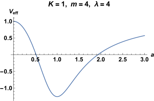
Figure 1: The effective potential for $K=1$, $m=4$ and $\lambda=4$. The universe expands and contracts in the region where $V_{eff}<0$ (with $\dot{a}^{2}=-V_{eff}$), with a bounce and a turnaround where $V_{eff}=0$.

As illustrated in Fig. 2, and as can be read off from (101), a variety of scenarios can be arranged by dialling $m$ and $\Lambda$. Specifically, by changing $m$ and $\lambda$ we can make the bounce as close to zero as required, and the expansion cycle as large as wanted.

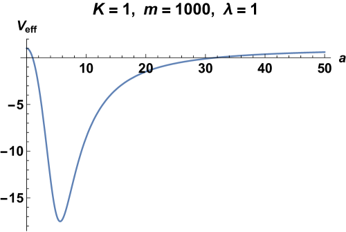
Figure 2: The effective potential for $K=1$, $m=1000$ and $\lambda=4$. As we see by dialing $m$ and $\lambda$ we can make the bounce as close to zero as required, and the expansion cycle as large as desired.

On the other extreme, by setting $\lambda m=4$, we obtain a static universe with:

$$a=\sqrt{\frac{\Lambda}{6}}.$$ (102)

Not only are these conditions different from the usual Einstein static universe static , but also, as expected from the behaviour when $\lambda m>4$, we see that such a static universe is stable. The effective potential is depicted in Fig. 3 for this case.

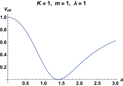
Figure 3: The effective potential for extremal case $K=1$, $m=1$ and $\lambda=4$. As the picture shows, a stable static Universe is found in this case.

IX.2 A single sign switch and two on/off switches

The only other situation where qualitative novelties are found is when one constant or term is subject to a sign switch and the other two have an on/off switch within the algebra of $SU(2)$. Three different cases can be listed:

IX.2.1 Case I

The most interesting follows from querying the sign of the gravitational constant and also whether $K$ and $\Lambda$ are switched off or on (and set to whatever non-zero value). Then, the Friedmann equation is:

$$H^{2}=-\frac{K}{2a^{2}}+\frac{\lambda}{2}+S\sqrt{\frac{m^{2}}{a^{8}}+\frac{1}{4a^{4}}+\frac{\lambda^{2}}{4}},$$ (103)

for the RHS of which we find a single zero at:

$$a=\left(\frac{2m^{2}}{-K\lambda}\right)^{\frac{1}{6}},$$ (104)

if $S=-1$ and $K\Lambda<0$. By drawing the effective potential (see Fig. 4) we see that it corresponds to a bounce for $K=-1$, $\Lambda>0$ and $S=-1$. A bounce is found; however, in this case there is no turnaround and recollapse. Nonetheless, the cosmological singularity appears to be removed here – no doubt due to the uncertainty in the sign of $G$ early on. Note that, for $K=1$, $\Lambda<0$ and $S=1,$ there is also a root, but it corresponds to a turnaround, since the effective potential is minus that in Figure 4. This would be no different from the standard case.

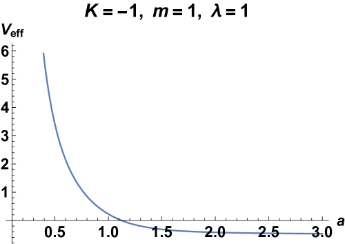
Figure 4: The effective potential when we query the sign of the gravitational constant and also whether $K$ and $\Lambda$ are switched off or on, with $K=-1$, $m=1$ and $\lambda=1$. A bounce is found, but in this case there is no turnaround at a maximum and subsequent recollapse.

IX.2.2 Case II

It could also be that we cannot know simultaneously whether $K=\pm 1$, and whether $G$ and $\Lambda$ are switched on or off. The sign issue therefore concerns the spatial curvature $K$, which we know to be non-zero, but quantum mechanically can be a superposition of $K=1$ and $K=-1$. Then, the Friedmann equation resulting from the diagonalized hamiltonian becomes:

$$H^{2}=\frac{m}{2a^{4}}+\frac{\lambda}{2}+S\sqrt{\frac{m^{2}}{4a^{8}}+\frac{1}{a^{4}}+\frac{\lambda^{2}}{4}}.$$ (105)

Taking the $S=-1$ branch, we see that there are no solutions (the RHS is negative) unless $m\lambda=2$ in which case

$$H\equiv 0.$$ (106)

Therefore, we obtain static solutions for all $a$, with indifferent stability.

IX.2.3 Case III

Finally, let us query the sign of $\Lambda,$ and whether or not $G$ and $K$ are switched on (with $G>0$ and either $K=1$ or $K=-1$). The Friedmann equation becomes:

$$H^{2}=\frac{m}{2a^{4}}-\frac{K}{2a^{2}}+S\sqrt{\frac{m^{2}}{4a^{8}}-\frac{1}{4a^{4}}+\lambda^{2}}.$$ (107)

For the $S=-1$ branch, we have a single zero when $K=-1$:

$$a=\left(\frac{-mK}{2\lambda^{2}}\right)^{\frac{1}{6}}.$$ (108)

However, no novelties are found in this case. Plotting the effective potential (see Fig 5) we see that this zero corresponds to a turnaround. The singularity is still present.

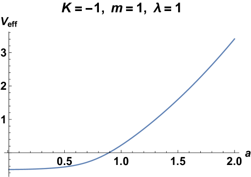
Figure 5: The effective potential when we query the sign of $\Lambda$ and also whether or not $G$ and $K$ are switched on, with $K=-1$, $m=1$ and $\lambda=1$.

In summary, there are striking qualitative novelties in the dynamics if we take the $S=-1$ state and use our formalism to switch on/off at least two of $K$, $G$ and $\Lambda$. One can see that in all other cases no new zeros for $\dot{a}$ are generated, the effects of the new dynamics limiting themselves to subtle differences in the transition regions between the eras when one of the 3 species dominates. If we take the $S=-1$ state, however, should we probe the on/off switch of $K$, $G$ and $\Lambda$ we find generically an early bounce. Ditto if we query the on/off switch of $K$ and $\Lambda$ and the sign of $G$. The only other case of any novelty was discussed in Section IX.2.2 and is highly contrived.

X Discussion

In this Section we briefly discuss the physical meaning of our model within the broader context of theories of the constants of Nature. We should clearly distinguish between variability (e.g. changes in space and time, or with energy, within a single universe) and diversity (where the constants remain fixed in each realization of the universe).

If we envisage theories with dynamical spacetime variations (for example Refs. BD ; B ; SBM ), then the variability (rather than the instantaneous, local numerical values) of dimensionful constants is meaningful because, even though the variations are tied to a system of units, its choice is pegged down by the dynamics (e.g. the lagrangian) given to the fields controlling the variations, typically rendered simple by that choice of units. Seen in another way, the dynamics yields dimensionful integration constants giving meaning to the variations. For example, in Brans-Dicke (BD) theory BD , the BD scalar field $\phi=G^{-1}$ is dimensionful but satisfies a second-order differential equation whose two constants of integration have the same dimensions, and their ratios with $\phi$ are trivially dimensionless, and so there is no confusion over Brans-Dicke being a theory for a varying dimensional constant ($G$).

Quite another situation arises when we imagine an ensemble of possible universes, each with its own set of fixed values for the constants, which then vary throughout the ensemble (such as in the Hilbert space proposed here, if all the operators associated with the constants commute). Then, their different numerical values are devoid of physical meaning if they produce the same dimensionless constants, and amount to nothing more than a rigid (i.e. fixed throughout each universe) change of units.

However, as this paper shows, we now see that, even in the latter context, if dimensionful constants are associated with operators that do not commute, the story changes. A physical meaning can be assigned to “diverse” dimensionful constants, because their complementarity precludes the naive hamiltonian evolution associated with them. A different operational dynamics arises from confronting the diversity of non-commuting constants.

A further contribution to this discussion can be extracted from the models presented in Section VIII. A change of units can never undo the information about the sign of a constant, or whether it has a zero or a non-zero value. This is true even before non-commutativity is applied to these models.

XI Conclusions

We have introduced a new approach to handling traditional physical constants in a quantum cosmological setting (quite different from either of the traditional ones quantum-cosmo ; loop-cosmo1 ; loop-cosmo2 ; vsl-cosmo ) by elevating constants of Nature to quantum operators in a kinematical Hilbert space. They do not have classical counterparts, and their commutators do not arise from classical Poisson brackets. Accordingly, the commutators of these constants do not endow them with any time evolution: in this sense they are the genuine constants – although their observed values are not fixed to take only a single set of values. We began by discussing the situation where the operators representing constants were commuting. In this case our proposal resembles the treatment given to classical parameters in quantum information theory – at least, if we live in an eigenstate of the constants. The possibility of non-commutativity introduces novelties, due to its associated uncertainty and complementarity principles – and may even preclude hamiltonian evolution. In this case the system typically evolves as a quantum superposition of hamiltonian evolutions resulting from a diagonalization process, and these are usually quite distinct from the original one (defined in terms of the non-commuting constants).

We presented several toy examples targeting $G$, $c$ and $\Lambda$, in the context of the dynamics of homogeneous and isotropic universes. If we base our construction on the Heisenberg algebra and the quantum harmonic oscillator, the alternative dynamics tend to silence matter (effectively setting $G$ to zero), and make the spatial curvature and the cosmological constant terms in the Friedmann equations act as if their signs are reversed. As a result, the early universe expands as a quantum superposition of different Milne or de Sitter metrics regardless of the material equation of state, even though the matter nominally dominates the density (in $\rho$ but not $G\rho$). A superposition of Einstein static universes was obtained as another worked example. We also investigated the results of basing our construction on the algebra of $SU(2)$, into which we can insert information about the sign of a constant of Nature, and whether its action is switched on or off. In this case we found examples displaying quantum superpositions of bounces in the initial state for the universe.

Our discussion has targeted the most interesting cases of quantising the constants $c,G$ and $\Lambda$ because they have immediate controlling consequences for the dynamics of homogeneous and isotropic universes. Other investigations can be made of cosmological models with different dynamics following the same quantum states of constants, where we have found that the quantum behaviour of simple anisotropies with isotropic 3-curvature does not reproduce that of massless scalar fields, as in the classical theory. In order to extend this approach to explore other constants, like the fine structure constant B ; SBM , the electron-proton mass ratio BMem , or the parameters defining the minimal standard model KMSM ; WSM , choices have to be made about possible non-commuting operator pairs. These extensions will be subjects for further work.

Another possible extension of this work concerns the classical limit of these theories, and what the wavefunction of the constants might be. It was suggested in notime that the parameter $\mathfrak{h}$ controlling non-commutativity (which need not be directly related to the usual $\hbar$) could be a function of the cosmic density ($\mathfrak{h}=\mathfrak{h}(\rho)$) and that below a certain density it could be pushed to zero, $\mathfrak{h}\rightarrow 0$, possibly at a phase transition. This could assist in bringing about classicality, but it might also require the wavefunction to be a coherent state in the original $\kappa_{1}$ and $\kappa_{2}$ in (24). The detailed construction of these states, however, is not straightforward. Note that they are not the naive coherent states built from $\alpha$ defined from (25) and (26), in fact, the latter are time dependent and form squeezed states in $\kappa_{1}$ and $\kappa_{2}$ at late times. This is because the transformation between the $\alpha_{i}$ and the $\kappa_{i}$ is time-dependent, with implications to be more thoroughly studied in a paper in preparation.

If the late-time dynamics is brought about by a phase transition which sets $\mathfrak{h}=0$, then no prediction is made for the late-time value of the constants (it is simply put in by hand when the appropriate coherent state is built). Likewise, there is no implication that a fundamental indeterminacy between constants might be at work at late times. However, the phase transition scenario is simply the minimal model, and further complexity could be built in. The issue of bringing about the late-time dynamics in our model would then be similar to the graceful exit problem in inflation, or the equivalent for all alternative scenarios. In such non-minimal models it is possible that the formalism proposed here would be at work nowadays, with interesting phenomenological implications. Such matters are left for further work. Note also that the issue of the collapse of the wave-function does not need to be addressed unless we are ready to embraced such non-minimal models.

To conclude we should stress that our constructions are not currently supported by any theory aspiring to the status of “fundamental” (such as string theory or loop quantum gravity). For example, there is no known fundamental principle specifying which constants should be included in the algebra of $SU(N)$ generalizing Section VIII. We are taking the first steps in a new direction and many questions are raised that we cannot yet answer. We hope that others will add to our beginnings and fill these gaps. In particular it would be interesting to see whether quantum gravity theories have anything to say in this respect. Although the discussion of matter coupling constants is hampered by the fact that most formalisms apply to vacuum dynamics only, a discussion of $\Lambda$ and $G$ should be possible. Some hints in this direction can be found in quantumlambda ; LeeGc .

XII Acknowledgements

We thank Stephon Alexander, David Jennings and Lee Smolin for discussions on matters related to this paper and Remo Garattini and Sabine Hossenfelder for bringing to our attention the connection between their work and ours. JDB and JM were both supported by consolidated grants from the Science and Technology Facilities Council (STFC) of the UK.

References

- (1) A. Einstein, Letter to I. Rosenthal-Schneider (30 March 1947), English translation in I. Rosenthal-Schneider, Reality and Scientific Truth, Wayne State Press, Detroit, 1980, pp. 56-7 and J.D. Barrow, The Constants of Nature, Bodley Head, London (2002), pp. 33-42.
- (2) H. Ooguri and C. Vafa, Nucl. Phys. B 766, 21 (2007); C. Vafa, The string landscape and the swampland, arXiv:hep-th/0509212; T. D. Brennan, F. Carta, and C. Vafa, The String Landscape, the Swampland, and the Missing Corner, arXiv:1711.00864
- (3) J.D. Barrow, Phys. Rev. D 71, 083520 (2005)
- (4) P. G. O. Freund, Nucl. Phys. B209, 146 (1982); E. W. Kolb, M. J. Perry, and T. P. Walker, Phys. Rev. D 33, 869 (1986); J.D. Barrow, Phys. Rev. D 35, 1805 (1987)
- (5) J.K. Webb, M.T. Murphy, V.V. Flambaum, V.A. Dzuba, J.D. Barrow, C.W. Churchill, J.X. Prochaska, and A.M. Wolfe. Phys. Rev. Lett. 87, 091301 (2001); J.A. King, J.K. Webb, M.T. Murphy, V.V. Flambaum, R.F. Carswell, M.B. Bainbridge, M.R. Wilczynska, and F.E. Koch, Mon. Not. Roy. astron. Soc. 422, 3370 (2012)
- (6) C. Brans and R.H. Dicke, Phys. Rev. 124, 925 (1961)
- (7) J.D. Bekenstein, Phys. Rev. D 25, 1527 (1982)
- (8) H.B. Sandvik, J.D. Barrow and J. Magueijo, Phys. Rev. Lett. 88, 031302 (2002)
- (9) G. Chiribella and R.W. Spekkens, (eds), Quantum Theory: Informational Foundations and Foils, Springer, New York (2016)
- (10) S. Alexander, J. Magueijo and L. Smolin, The quantum cosmological constant, arXiv:1807.01381
- (11) J. Magueijo and L. Smolin, A universe that does not know the time, arXiv:1807.01520
- (12) R. Garattini, J. Phys. A 39, 6393 (2006) doi:10.1088/0305-4470/39/21/S33 [gr-qc/0510061].
- (13) B. Carr, (ed.) Universe or Multiverse?, Cambridge UP, Cambridge, (2007)
- (14) S. Hossenfelder, Found. Phys. 42, 1452 (2012) doi:10.1007/s10701-012-9678-0 [arXiv:1207.1002 [gr-qc]].
- (15) J.D. Barrow, Observatory 113, 210 (1993)
- (16) J.D. Barrow, G.F.R. Ellis, R. Maartens, and C.G. Tsagas, Class. Quantum Gravity 20, L155 (2003).
- (17) J. J. Halliwell, In Jerusalem 1989, Proceedings, Quantum cosmology and baby universes 159-243 and MIT Cambridge - CTP-1845, gr-qc/0909.2566
- (18) A. Ashtekar, Lect. Notes Phys. 863, 31 (2013)
- (19) M. Bojowald, Rept. Prog. Phys. 78, 023901 (2015)
- (20) A. Balcerzak, JCAP 1504, 019 (2015).
- (21) J. D. Barrow and J. Magueijo, Phys. Rev. D 72, 043521 (2005) doi:10.1103/PhysRevD.72.043521 [astro-ph/0503222].
- (22) D. Kimberly and J. Magueijo, Phys. Lett. B 584, 8 (2004) doi:10.1016/j.physletb.2004.01.050 [hep-ph/0310030].
- (23) F. Wilczek, arXiv:0708.4361 [hep-ph].
- (24) L. Smolin, Class. Quant. Grav. 33, no. 2, 025011 (2016), [arXiv:1507.01229 [hep-th]].