Quark jets scattering from a gluon field: from saturation to high $p_{t}$

Abstract

We continue our studies of possible generalization of the Color Glass Condensate (CGC) effective theory of high energy QCD to include the high $p_{t}$ (or equivalently large $x$) QCD dynamics as proposed in [1]. Here we consider scattering of a quark from both the small and large $x$ gluon degrees of freedom in a proton or nucleus target and derive the full scattering amplitude by including the interactions between the small and large $x$ gluons of the target. We thus generalize the standard eikonal approximation for parton scattering which can now be deflected by a large angle (and therefore have large $p_{t}$) and also lose a significant fraction of its longitudinal momentum (unlike the eikonal approximation). The corresponding production cross section can thus serve as the starting point toward derivation of a general evolution equation that would contain DGLAP evolution equation at large $Q^{2}$ and the JIMWLK evolution equation at small $x$. This amplitude can also be used to construct the quark Feynman propagator which is the first ingredient needed to generalize the Color Glass Condensate (CGC) effective theory of high energy QCD to include the high $p_{t}$ dynamics. We outline how it can be used to compute observables in the large $x$ (high $p_{t}$) kinematic region where the standard Color Glass Condensate formalism breaks down.

1 Introduction

Twist expansion and collinear factorization approach [2] to particle production in QCD is a powerful and extremely useful formalism for particle production in high energy hadronic/nuclear collisions at high $p_{t}$. However it is not expected to be valid at high energy and/or for large nuclei where twist expansion breaks down due to high gluon density effects (gluon saturation). The Color Glass Condensate (CGC) formalism (see [3] for reviews) is an effective field theory approach to QCD at high energies which relies on the fact that at high energy (or at small $x$) a hadron or nucleus wave function contains many gluons, referred to as gluon saturation [4, 5], and hence is a dense many-body system which is most efficiently described via semi-classical methods [6]. The most significant aspect of CGC is perhaps the emergence of a dynamical scale, called the saturation scale $Q_{s}$ , which grows with energy (or $1/x$) and hence can be semi-hard. The CGC formalism thus can be used to compute quantities such as gluon multiplicities,… which are not amenable to the standard perturbative methods. Even though applications of the CGC formalism to hadronic/nuclear processes in a limited range of kinematics at RHIC and the LHC have been quite successful [7], the CGC formalism has its shortcomings, namely it is not valid when one probes large $x$ modes of the target proton or nucleus. In case of particle production in hadronic collisions this happens when high $p_{t}$ particles are produced since $x$ and $p_{t}$ are kinematically related, $x\sim{p_{t}\over\sqrt{s}}$. This is specially important for particle production in mid rapidity as well as the Large Hadron Collider (LHC) where due to the large center of mass energy of the collision a large range of transverse momentum becomes accessible. Furthermore, the large $x$ region will be the dominant part of kinematics covered in the proposed Electron Ion Collider (EIC), at least in the earliest stages [8]. Therefore it is desirable to devise a formalism that not only incorporates the physics of saturation but also has the correct high $p_{t}$ and/or large $x$ physics encoded.

Generalizing the CGC formalism to include high $p_{t}$ physics would have significant ramifications not only for saturation physics and the work to determine its domain of applicability, it would also enable one to describe a wide range of phenomena using the same formalism. For example, saturation physics is commonly employed to provide the initial conditions for the hydrodynamic evolution of the medium, the Quark Gluon Plasma, created in high energy heavy ion collisions but is not applicable to jet (radiative) energy loss and the interactions between high $p_{t}$ partons and the produced medium. Elastic energy loss and loss (shift) of rapidity are also not present in the current formulation of saturation physics but must be included in a more general description which could be specially significant for cold matter energy loss and $p_{t}$ broadening.

Toward this goal we proposed a more general approach in [1]. We considered a high energy quark scattering from a target proton or nucleus whereas the quark not only scatters from the small $x$ gluons of the target, represented by a soft color field, but also from the large $x$ gluons in the target. We resummed the multiple scatterings of the quark from the soft classical fields to all orders in the number of soft scatterings but kept only the first scattering from the large $x$ modes. However we did not consider the large $x$ modes themselves scattering from the small $x$ gluons. Here we continue this approach and proceed to include interactions between the large $x$ gluons and the soft background field representing small $x$ gluons of the target.

We start by a brief overview of the approximations used in high energy (eikonal) scattering and how it is used in saturation physics when viewed in the target rest frame. We then give a brief summary of the approximations and the methods used in our approach in [1]. We again consider scattering of a quark from a proton or nucleus target including both small and large $x$ gluon modes. We then proceed to calculate and resum multiple interactions between the small $x$ color fields and the large $x$ gluons in the target. We then briefly outline how the calculated scattering amplitude may be used to extract the quark propagator in this more general setting and how the quark propagator may be used to compute physical observables in full range of $x$ (and/or $p_{t}$).

2 Eikonal approximation, multiple scattering at small $x$ and beyond

Here we remind the reader of the approximations involved in high energy (eikonal) scattering. As this is standard and already covered in detail in [1] we will be brief here. We define the light cone coordinates as

$$x^{+}\equiv{t+z\over\sqrt{2}}\,\,,\,\,x^{-}\equiv{t-z\over\sqrt{2}}$$ (1)

and similarly for momenta and fields. The small $x$ gluons of the target are modeled as a soft color (background) field $S_{a}^{\mu}(x)$. One can either work in the frame where both the projectile and the target are moving fast, or in the frame where the projectile quark is fast and the target is at rest. In either frame the projectile quark moving to the right (along the $x^{+}$ direction to be specific) will have a large $p^{+}$ component of momentum and will couple to the conjugate component of the target color field $S^{-}$. Furthermore, the target color field is independent of $x^{-}$ so that $S_{a}^{-}=S_{a}^{-}(x^{+},x_{t})$. We also define a light-like vector

$$n^{\mu}=(n^{+}=0,n^{-}=1,n_{t}=0)$$ (2)

with $n^{2}=0$ which can be used to extract the Lorentz index of the soft color field and express it as $S^{-}_{a}\equiv n^{-}\,S_{a}(x^{+},x_{t})$ so that $\raise 0.6458pt\hbox{$/$}\kern-7.29996pt\hbox{$S$}_{a}=S_{s}^{\mu}\,\gamma_{\mu}=\raise 0.6458pt\hbox{$/$}\kern-5.29999pt\hbox{$n$}\,S_{a}$ which will help keep the expressions compact.

The $n$-th order of the scattering of a quark, with momentum $p$, from the color field of the target is depicted in Fig. 1 (target is shown as an ellipse) where $x_{i}$ label the coordinate positions of the field $S^{-}$ in the target (one should think of this as the projectile quark multiply scattering while going right through the target so that there are no propagators between the quark line and the target field). Diagrams of this type resum into a path-ordered infinite Wilson line provided one neglects the transverse momenta of the intermediate quark lines and the phases one picks up after integrating over the $p^{-}_{i}$ of each intermediate quark propagator $p_{i}^{\mu}$. The integration over the minus component of the intermediate propagators forces a path ordering such that the scattering is sequential along the longitudinal direction, i.e., $x_{i}^{+}>x_{i-1}^{+}$ and so on (see [1, 9, 10] for details).

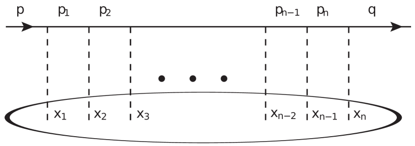
Figure 1: Multiple soft scatterings from the color field of the target.

The scattering amplitude can then be written as

$$i\mathcal{M}_{eikonal}(p,q)=2\pi\delta(p^{+}-q^{+})\,\bar{u}(q)\,\raise 0.6458pt\hbox{$/$}\kern-5.29999pt\hbox{$n$}\,\int d^{2}x_{t}\,e^{-i(q_{t}-p_{t})\cdot x_{t}}\,\left[V(x_{t})-1\right]\,u(p)$$ (3)

where the infinite Wilson line $V(x_{t})$ is defined as

$$V(x_{t})\equiv\hat{P}\,\exp\left\{ig\int_{-\infty}^{+\infty}dx^{+}\,S^{-}_{a}(x^{+},x_{t})\,t_{a}\right\}$$ (4)

and depicted in Fig. 2.

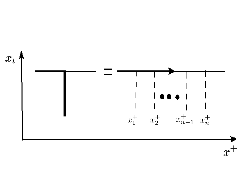
Figure 2: A Wilson line representing eikonal scattering of a high energy quark.

This infinite Wilson line resums multiple scatterings of a high energy quark (moving along the positive $z$ axis) on a soft background color field to all orders in the soft field $\left[ig\,S_{a}\,t_{a}\right]^{n}$. Due to the eikonal approximation (see also [11] where the first energy suppressed terms are investigated) the transverse position of the quark does not change during the scattering, i.e., the projectile quark does not get a significant deflection (small angle scattering). Color matrices $t_{a}$ are in the fundamental representation and soft color field $S^{-}$ represents small $x$ gluon modes of the target.

In [1] we went beyond eikonal approximation by including scattering from a large $x$ gluon field denoted $A^{\mu}(x)$ which, unlike the soft field $S^{-}$, carries large longitudinal momentum and can therefore cause a large deflection of the projectile quark. Due to the possibility of this large angle deflection (so that the final state quark has a large transverse momentum) it was necessary to introduce a rotated frame, denoted bar-ed frame, where the scattered quark is moving along a new longitudinal direction $\bar{z}$. The bar-ed coordinates are related to the original $x,y,z$ coordinates (projectile quark is moving along the $z$ direction) via the rotation matrix $\mathcal{O}$ in $3$ dimensions.

$$\left(\begin{array}[]{c}\bar{x}\\ \bar{y}\\ \bar{z}\end{array}\right)=\mathcal{O}\,\left(\begin{array}[]{c}x\\ y\\ z\end{array}\right)$$ (5)

The elements of this $3$-d rotation matrix are expressed in terms of the $3$-momentum of the scattered quark. We also defined a new light cone vector $\bar{n}$ which projects out the plus component in the new frame, so that $\bar{n}\cdot\bar{p}=\bar{p}^{+}$. We then managed to resum all the multiple scatterings of the projectile quark from the soft field and one scattering from the large $x$ (sometimes referred to as the hard field where hard refers to a large longitudinal momentum). This is shown in Fig. 3 (target is not explicitly drawn),

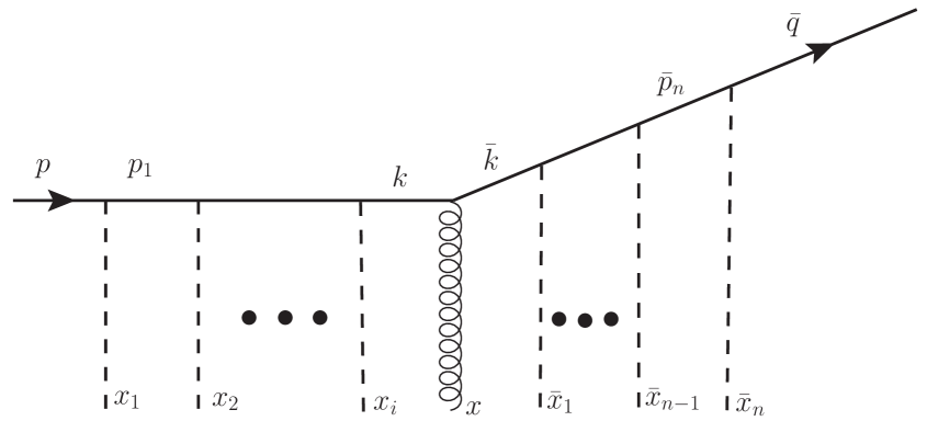
Figure 3: Multiple soft scatterings before and after a hard one at $x$.

Diagrams of this type resum into [1]

$$i\mathcal{M}_{1} = \int d^{4}x\,d^{2}z_{t}\,d^{2}\bar{z}_{t}\,\int{d^{2}k_{t}\over(2\pi)^{2}}\,{d^{2}\bar{k}_{t}\over(2\pi)^{2}}\,e^{i(\bar{k}-k)x}\,e^{-i(\bar{q}_{t}-\bar{k}_{t})\cdot\bar{z}_{t}}\,e^{-i(k_{t}-p_{t})\cdot z_{t}}$$ (6)

$$\bar{u}(\bar{q})\,\left[\overline{V}_{AP}(x^{+},\bar{z}_{t})\,\raise 0.6458pt\hbox{$/$}\kern-5.29999pt\hbox{$\bar{n}$}\,{\raise 0.6458pt\hbox{$/$}\kern-5.29999pt\hbox{$\bar{k}$}\over 2\bar{k}^{+}}\,\left[ig\,\raise 0.6458pt\hbox{$/$}\kern-7.29996pt\hbox{$A$}(x)\right]\,{\raise 0.6458pt\hbox{$/$}\kern-5.29999pt\hbox{$k$}\over 2k^{+}}\,\raise 0.6458pt\hbox{$/$}\kern-5.29999pt\hbox{$n$}\,V_{AP}(z_{t},x^{+})\right]\,u(p)$$

with $k^{+}=p^{+},k^{-}={k_{t}^{2}\over 2k^{+}}$, $\bar{k}^{+}=\bar{q}^{+},\bar{k}^{-}={\bar{k}_{t}^{2}\over 2\bar{k}^{+}}$ and the semi-infinite, anti path-ordered Wilson lines in the fundamental representation are now defined as 

$$\overline{V}_{AP}(x^{+},\bar{z}_{t})\equiv\hat{P}\,\exp\left\{ig\int_{x^{+}}^{+\infty}d\bar{z}^{+}\,\bar{S}^{-}_{a}(\bar{z}_{t},\bar{z}^{+})\,t_{a}\right\}$$ (7)

and

$$V_{AP}(z_{t},x^{+})\equiv\hat{P}\,\exp\left\{ig\int_{-\infty}^{x^{+}}dz^{+}\,S^{-}_{a}(z_{t},z^{+})\,t_{a}\right\}.$$ (8)

where anti path-ordering (AP) in the amplitude means fields with the largest argument appear to the left.

2.1 Multiple scatterings of the large $x$ gluon

We now proceed to consider interactions of the hard (large $x$) gluon with the soft background field. First let us consider the case when only the hard gluon interacts with the soft field but not the initial or final state quark, as shown in Fig. 4

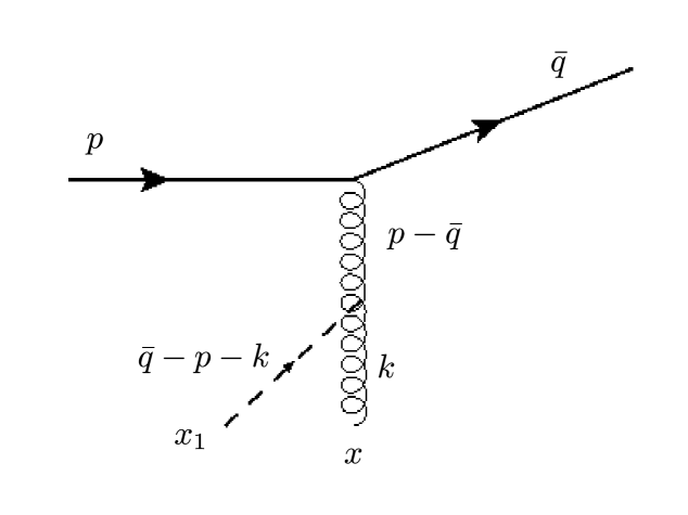
Figure 4: One soft scattering of the large $x$ gluon.

The amplitude can be written as

$$i\mathcal{M} = \int{d^{4}k\over(2\pi)^{4}}\,d^{4}x\,d^{4}x_{1}\,e^{i(\bar{q}-p-k)x_{1}}\,e^{ikx}\,\bar{u}(\bar{q})\,(ig\,\gamma^{\mu}\,t^{a})\,u(p)$$

$$G_{\mu\nu}^{ab}(p-\bar{q})\,V^{\nu\,\lambda\rho}_{bcd}(p-\bar{q},k,\bar{q}-p-k)A_{\lambda}^{c}(x)\,\left[i\,g\,S_{\rho}^{d}(x_{1})\right]$$

where the free gluon propagator is

$$G^{\mu\nu}_{ab}(l)={i\delta_{ab}\over l^{2}+i\epsilon}\,\left[-g^{\mu\nu}+{n^{\mu}\,l^{\nu}+l^{\mu}\,n^{\nu}\over n\cdot l}\right]$$ (9)

and the triple gluon vertex is

$$V^{bcd}_{\nu\lambda\rho}(l_{1},l_{2},l_{3})=g\,f^{bcd}\,\left[(l_{2}-l_{3})_{\nu}\,g_{\lambda\rho}+(l_{3}-l_{1})_{\lambda}\,g_{\rho\nu}+(l_{1}-l_{2})_{\rho}\,g_{\nu\lambda}\right]$$ (10)

The large $x$ gluon field is denoted $A(x^{+},x^{-},x_{t})$ while the soft field is $S^{-}_{d}(x_{1}^{+},x_{1t})=n^{-}\,S_{d}(x_{1}^{+},x_{1t})$. It is straightforward to simplify the Lorentz structure of the amplitude by repeated use of the gauge condition $n\cdot A=0$ as well as the null condition $n^{2}=0$ and the fact that the soft field has only a $-$ component and therefore is proportional to $n^{\mu}$. We get

$$i\mathcal{M} = f_{acd}\,\int{d^{4}k\over(2\pi)^{4}}\,d^{4}x\,d^{4}x_{1}\,e^{i(\bar{q}-p-k)x_{1}}\,e^{ikx}\,\bar{u}(\bar{q})\,(ig\,\gamma^{\mu}\,t^{a})\,u(p)\,A_{\lambda}^{c}(x)\,\left[i\,g\,S^{d}(x_{1})\right]$$ (11)

$${1\over(p-\bar{q})^{2}+i\epsilon}\,\left[-g^{\mu}_{\lambda}\,n\cdot(p-\bar{q}-k)+n^{\mu}\,(p-\bar{q}_{\lambda}\,(1-{n\cdot k\over n\cdot(p-\bar{q})})\right]$$

As before the soft field $S$ is independent of the $x_{1}^{-}$ coordinate which allows us to do the integration over $x_{1}^{-}$ coordinate which gives $\delta(\bar{q}^{+}-p^{+}-k^{+})$ which in turn is used to do the $k^{+}$ integration setting $k^{+}=\bar{q}^{+}-p^{+}$ upon integrating $k^{+}$. We also note that the only $k$ dependence left is in the phase factors since $n\cdot k$ kills all the other possible $k$ dependent terms. Then one can carry out the $k_{t}$ and $k^{-}$ integrations which lead to delta functions $\delta^{2}(x_{1t}-x_{t})\,\delta(x_{1}^{+}-x^{+})$ which are then used to perform the remaining integrations over $x_{1}^{+},x_{1t}$ setting $x_{1t}=x_{t}$ and $x_{1}^{+}=x^{+}$. In other words the soft field $S$ and the large $x$ (hard) field $A$ are at the same space coordinate except that the soft field $S$ does not depend on $x^{-}$, unlike the hard field $A$. After performing the above integrations we are left with

$$i\mathcal{M} = 2f_{acd}\,\int\,d^{4}x\,e^{i(\bar{q}-p)x}\,\bar{u}(\bar{q})\,{\left[\raise 0.6458pt\hbox{$/$}\kern-5.29999pt\hbox{$n$}\,(p-\bar{q})\cdot A_{c}(x)-\raise 0.6458pt\hbox{$/$}\kern-7.29996pt\hbox{$A$}_{c}(x)\,n\cdot(p-\bar{q})\right]\over(p-\bar{q})^{2}}\,(ig\,t^{a})\,u(p)$$ (12)

$$\left[i\,g\,S^{d}(x^{+},x_{t})\right]$$

with the most important point being the soft and hard field are at the same point. We now go ahead and consider one more soft scattering of the hard gluon as shown in Fig. 5,

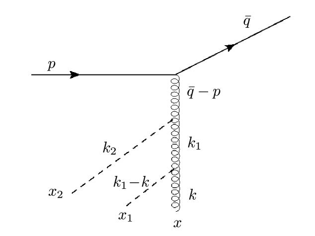
Figure 5: Two soft scatterings of the large $x$ gluon.

We can now repeat the same steps as before, using the gauge choice and the null vector condition to simplify the Lorentz structure, performing the integration over $k$ puts the fields $A$ and $S(x_{1})$ at the same point ($x_{1}=x$) as before, however there is now an integration over $k_{1}$. Let us now consider the $k_{1}^{-}$ integration,

$$I\equiv\int{dk^{-}_{1}\over(2\pi)}\,{e^{ik_{1}^{-}(x^{+}-x_{2}^{+})}\over 2(\bar{q}^{+}-p^{+})\left[k_{1}^{-}-{k_{1t}^{2}-i\epsilon\over 2(\bar{q}^{+}-p^{+})}\right]}$$ (13)

This integration can be done using the standard contour integration techniques realizing that the $k_{1}^{-}$ pole is always below the real axis since $p^{+}>\bar{q}^{+}$. This integral is then

$$I\sim{i\,\theta(x^{+}-x_{2}^{+})\over 2n\cdot(\bar{q}-p)}\,e^{i{k_{1t}^{2}\over 2n\cdot(\bar{q}-p)}(x^{+}-x_{2}^{+})}\,.$$ (14)

The most essential point here is the reappearance of the theta function $\theta(x^{+}-x_{2}^{+})$ which forces a path ordering of the soft scatterings. This is not surprising since the soft multiple scatterings are eikonal. The rest of the analysis goes through as before and we get

$$i\mathcal{M} = 2\,f_{abc}\,f_{cde}\int\,d^{4}x\,dx_{2}^{+}\,\theta(x^{+}-x_{2}^{+})\,e^{i(\bar{q}-p)x}$$ (15)

$$\bar{u}(\bar{q})\,{\left[\raise 0.6458pt\hbox{$/$}\kern-5.29999pt\hbox{$n$}\,(p-\bar{q})\cdot A_{e}(x)-\raise 0.6458pt\hbox{$/$}\kern-7.29996pt\hbox{$A$}_{c}(x)\,n\cdot(p-\bar{q})\right]\over(p-\bar{q})^{2}}\,(ig\,t^{a})\,u(p)$$

$$\left[i\,g\,S_{d}(x^{+},x_{t})\right]\,\left[i\,g\,S_{b}(x_{2}^{+},x_{t})\right]$$

Including more soft scattering on the hard gluon line is straightforward and proceeds as usual, with each extra soft scattering path ordered. This allows one to resum all the soft scatterings of the hard gluon and write it as

$$i\mathcal{M}_{2} = {2\,i\over(p-\bar{q})^{2}}\,\int d^{4}x\,e^{i(\bar{q}-p)x}\,\bar{u}(\bar{q})\,\bigg{[}(ig\,t^{a})\,\left[\partial_{x^{+}}\,U_{AP}^{\dagger}(x_{t},x^{+})\right]^{ab}$$ (16)

$$\left[n\cdot(p-\bar{q})\,\raise 0.6458pt\hbox{$/$}\kern-7.29996pt\hbox{$A$}_{b}(x)-(p-\bar{q})\cdot A_{b}(x)\,\raise 0.6458pt\hbox{$/$}\kern-5.29999pt\hbox{$n$}\right]\,\bigg{]}\,u(p)$$

where the derivative acts on the $+$ coordinate of the adjoint Wilson line (anti path-ordered in the amplitude) and arises from the fact that one can write the soft field at the last scattering point as a derivative on the Wilson line. This amplitude is symbolically shown in Fig. 6 where the thick solid line attached to the hard gluon line depicts a semi-infinite (and anti path-ordered) Wilson line in the adjoint representation (analog of eq. (8)) .

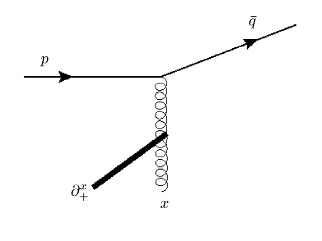
Figure 6: Multiple soft scatterings of the large $x$ gluon.

Finally we note that this amplitude vanishes in the soft (eikonal) limit, i.e. when $\bar{q}^{+}\rightarrow p^{+}$ and $A^{\mu}\rightarrow S^{-}$.

2.2 Multiple scatterings of the large $x$ gluon and the final state quark

We now consider the case when both the large $x$ gluon and the final state quark multiply scatter from the soft background field. The first diagram not included so far is when both the large $x$ gluon and the final state quark scatter once as shown in Fig. 7.

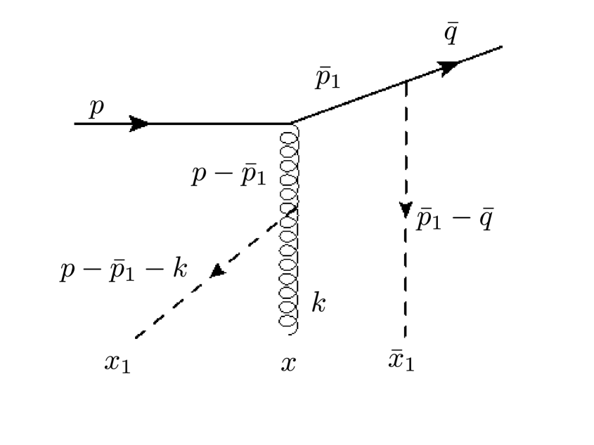
Figure 7: Both the large $x$ gluon and the final state quark scattering once.

This scattering amplitude is given by

$$i\mathcal{M} = \int{d^{4}k\over(2\pi)^{4}}\,{d^{4}\bar{p}_{1}\over(2\pi)^{4}}\,d^{4}x\,d^{4}x_{1}\,d^{4}\bar{x}_{1}\,e^{i(\bar{q}-\bar{p}_{1})\bar{x}_{1}}\,e^{-ikx}\,e^{-i(p-\bar{p}_{1}-k)x_{1}}\,\bar{u}(\bar{q})\,\raise 0.6458pt\hbox{$/$}\kern-5.29999pt\hbox{$\bar{n}$}$$

$$\left[i\,g\,\bar{S}(\bar{x}_{1})\right]\,{i\bar{\raise 0.6458pt\hbox{$/$}\kern-5.29999pt\hbox{$p$}}_{1}\over\bar{p}_{1}^{2}+i\epsilon}(ig\,\gamma^{\mu}\,t^{a})\,u(p)\,G_{\mu\nu}(p-\bar{p}_{1})\,V^{\nu\lambda\rho}_{abc}(p-\bar{p}_{1},-k,\bar{p}_{1}+k-p)$$

$$A_{\lambda}^{b}(x)\,\left[i\,g\,n_{\rho}\,S^{c}(x_{1})\right]$$

Many of the steps involved in simplifying this expression are identical to the previous ones, for example we use the fact that the soft field $S^{-}(x_{i})$ is independent of the $x_{i}^{-}$ coordinate to perform the integration over the minus components of their coordinates leading to delta functions relating the $+$ components of the momenta. The Lorentz structure can also be simplifies as before by repeated use of the gauge condition as well as the fact that $n^{2}=\bar{n}^{2}=0$ and that the soft fields (in their respective frames) have only minus components which allows extraction of their Lorentz index by the use of the light-like vectors $n$ and $\bar{n}$ so that $S^{-}=n^{-}\,S$ and $\bar{S}^{-}=\bar{n}^{-}\,\bar{S}$. As in the case of only the hard gluon scattering we just considered one gets $x_{1}^{+}=x^{+}$ and $x_{1t}=x_{t}$. The most important part is the integration over $\bar{p}^{-}_{1}$ momentum of the intermediate quark line which can be written as

$$I\sim\int{d\bar{p}^{-}_{1}\over(2\pi)}\,{e^{-i\bar{p}_{1}^{-}(\bar{x}_{1}^{+}-x^{+})}\over\left[\bar{p}_{1}^{-}-{\bar{p}_{1t}^{2}-i\epsilon\over 2\bar{q}^{+}}\right]\left[\bar{p}_{1}^{-}-p^{-}-{(\bar{p}_{1t}-p_{t})^{2}-i\epsilon\over 2(\bar{q}^{+}-p^{+})}\right]}$$ (17)

keeping in mind that both $p^{+},\bar{q}^{+}>0$ and that $p^{+}-\bar{q}^{+}>0$ we see that the integral above has two poles which are on the opposite side of the real axis. This is completely different from the eikonal scattering where the intermediate quark propagators have poles which are all on the same side of the real axis which leads to path ordering along the $+$ direction. This integral can be evaluated using the standard contour integration techniques and gives

$$I\sim\left[\theta(\bar{x}_{1}^{+}-x^{+})\,e^{-i{\bar{p}_{1t}^{2}\over 2\bar{q}^{+}}(\bar{x}_{1}^{+}-x^{+})}+\theta(x^{+}-\bar{x}_{1}^{+})\,e^{-i\left[p^{-}+{(\bar{p}_{1t}-p_{t})^{2}\over 2(\bar{q}^{+}-p^{+})}\right](\bar{x}_{1}^{+}-x^{+})}\right]$$ (18)

To proceed further and to stay consistent with the approximations made for strict eikonal scattering where one neglects terms of the order ${p_{t}\over p^{+}}$ we will ignore the phase factors above. We then see that the two different path orderings corresponding to the two theta functions add to unity and path ordering disappears. This can be understood as the following, integration over any of the poles forces the other propagator to go off-shell and to become space-like in which case there is no absolute ordering between the interaction vertices at $x_{1}^{+}=x^{+}$ and $\bar{x}_{1}^{+}$. However, if we consider further soft scatterings of the hard gluon and the final state quark they will be path ordered with respect to $x^{+}$ and $\bar{x}_{1}^{+}$ respectively. This is straightforward but long and we will just quote the final result as the calculations proceeds as earlier and there are no further subtle points. Resuming all the soft scatterings of the hard gluon and the final state quark then gives

$$i\mathcal{M}_{3} \!\!=\!\! -2\,i\,\int d^{4}x\,d^{2}\bar{x}_{t}\,d\bar{x}^{+}\,{d^{2}\bar{p}_{1t}\over(2\pi)^{2}}\,e^{i(\bar{q}^{+}-p^{+})x^{-}}\,e^{-i(\bar{p}_{1t}-p_{t})\cdot x_{t}}\,e^{-i(\bar{q}_{t}-\bar{p}_{1t})\cdot\bar{x}_{t}}$$ (19)

$$\bar{u}(\bar{q})\,\bigg{[}\left[\partial_{\bar{x}^{+}}\,\overline{V}_{AP}(\bar{x}^{+},\bar{x}_{t})\right]\,\raise 0.6458pt\hbox{$/$}\kern-5.29999pt\hbox{$\bar{n}$}\,\raise 0.6458pt\hbox{$/$}\kern-5.29999pt\hbox{$\bar{p}_{1}$}\,(igt^{a})\,\left[\partial_{x^{+}}\,U^{\dagger}_{AP}(x_{t},x^{+})\right]^{ab}$$

$${\left[n\cdot(p-\bar{q})\,\raise 0.6458pt\hbox{$/$}\kern-7.29996pt\hbox{$A$}^{b}(x)-(p-\bar{p}_{1})\cdot A^{b}(x)\,\raise 0.6458pt\hbox{$/$}\kern-5.29999pt\hbox{$n$}\right]\over\left[2n\cdot\bar{q}\,2n\cdot(p-\bar{q})\,p^{-}-2n\cdot(p-\bar{q})\,\bar{p}^{2}_{1t}-2n\cdot\bar{q}\,(\bar{p}_{1t}-p_{t})^{2}\right]}\bigg{]}\,u(p)$$

and is depicted in Fig. 8 below where the thick solid lines denote semi-infinite (and anti path-ordered) Wilson lines in fundamental (attached to the final state quark line) and adjoint (attached to the hard gluon line) representations. Also, we have $\bar{p}_{1}^{+}=\bar{q}^{+}$. We again note that this amplitude also vanishes in the soft limit.

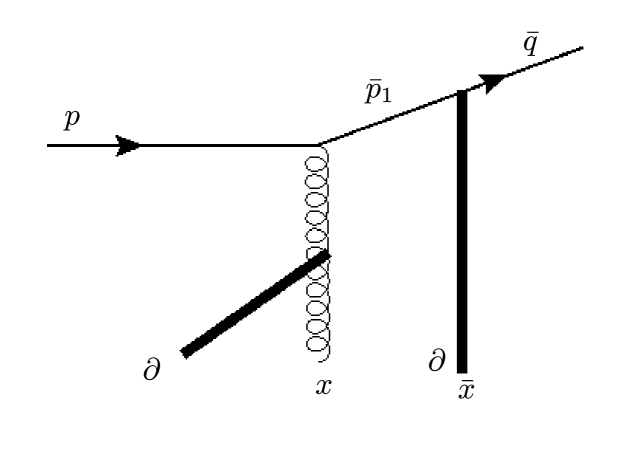
Figure 8: Soft scatterings of the final state quark and the large $x$ gluon.

2.3 Multiple scatterings of the initial state quark and the large $x$ gluon

We now consider the next class of diagrams in which both the large $x$ gluon and the initial state quark scatter from the soft background field. The lowest order diagram, not included so far, is shown in Fig. 9 below

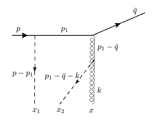
Figure 9: Soft scatterings of the initial state quark and the large $x$ gluon.

This amplitude can be written as

$$i\mathcal{M} = \int{d^{4}k\over(2\pi)^{4}}\,{d^{4}p_{1}\over(2\pi)^{4}}\,d^{4}x\,d^{4}x_{1}\,d^{4}x_{2}\,e^{i(p_{1}-p)x_{1}}\,e^{-ikx}\,e^{i(k+\bar{q}-p_{1})x_{2}}$$

$$\left[\bar{u}(\bar{q})\,(ig\,\gamma^{\mu}\,t^{a})\,{i\raise 0.6458pt\hbox{$/$}\kern-5.29999pt\hbox{$p$}_{1}\over p_{1}^{2}+i\epsilon}\,\raise 0.6458pt\hbox{$/$}\kern-5.29999pt\hbox{$n$}\,\left[i\,g\,S(x_{1})\right]\,u(p)\right]\,G_{\mu\nu}(p_{1}-\bar{q})$$

$$V^{\nu\lambda\rho}_{acd}(p_{1}-\bar{q},-k,k+\bar{q}-p_{1})\,A_{\lambda}^{c}(x)\,\left[i\,g\,n_{\rho}\,S^{d}(x_{2})\right]$$

Again most of the steps are identical to before; one integrates over $-$ component of the soft fields coordinates, eventually setting some $+$ components of momenta equal to each other. Lorentz structure is simplified using the gauge condition and the null vector $n^{2}=0$ as well as extracting the Lorentz index of the soft field $S^{-}=n^{\mu}\,S$. Integration over $k$ again sets $x^{+}_{2}=x^{+}$. The crucial step now is the integration over $p_{1}^{-}$ which we focus on,

$$I\sim\int{dp^{-}_{1}\over(2\pi)}\,{e^{-ip_{1}^{-}(x_{1}^{+}-x^{+})}\over\left[p_{1}^{-}-{p_{1t}^{2}-i\epsilon\over 2p^{+}}\right]\left[p_{1}^{-}-\bar{q}^{-}-{(p_{1t}-\bar{q}_{t})^{2}-i\epsilon\over 2(p^{+}-\bar{q}^{+})}\right]}$$ (20)

The two poles are now both below the real axis so that the integration gives a non-zero value only if $x^{+}>x_{1}^{+}$, we get

$$I\sim\theta(x^{+}-x_{1}^{+})\,\left[e^{i{p_{1t}^{2}\over 2p^{+}}(x_{1}^{+}-x^{+})}-\,e^{i\left[\bar{q}^{-}+{(p_{1t}-\bar{q}_{t})^{2}\over 2(p^{+}-\bar{q}^{+})}\right](x_{1}^{+}-x^{+})}\right]$$ (21)

now, unlike in the case of scattering from the large $x$ gluon and the final state quark, the relative sign between the two phase factors is negative (recall that the poles were on the opposite side in that case). Hence ignoring the phases again consistent with strict eikonal approximation, one gets a cancellation between the two terms so that $I=0$, therefore this amplitude identically vanishes! It is straightforward to include any number of further soft scatterings from the initial or final state quark or the large $x$ gluon. However, it can be shown these further scatterings do not affect this null result. Therefore we conclude that one can not have simultaneous soft scatterings from the initial state quark and the large $x$ gluon. There are no other diagrams to consider, therefore this completes our derivation of the amplitude for scattering of a quark from the small and large $x$ gluon fields of the target.

The result for the full scattering amplitude at all $x$ (or any $p_{t}$) can thus be written as

$$i\mathcal{M}=i\mathcal{M}_{eikonal}+i\mathcal{M}_{1}+i\mathcal{M}_{2}+i\mathcal{M}_{3}$$ (22)

where $i\mathcal{M}_{eikonal}$, $i\mathcal{M}_{1}$, $i\mathcal{M}_{2}$ and $i\mathcal{M}_{3}$ are given by eqs. (3,6,16,19) respectively. This is our main result. We further recall [1] that one needs to use the covariant coupling in the large $x$ terms so that the above amplitude smoothly reduces to the eikonal amplitude $i\mathcal{M}_{eikonal}$ in the soft scattering limit, i.e. when $\raise 0.6458pt\hbox{$/$}\kern-7.29996pt\hbox{$A$}(x^{+},x^{-},x_{t})\rightarrow\raise 0.6458pt\hbox{$/$}\kern-5.29999pt\hbox{$n$}\,S(x^{+},x_{t})$. To extract the quark propagator one defines the effective vertex $\tau_{F}$ as

$$i\mathcal{M}(p,\bar{q})=\bar{u}(\bar{q})\,\tau_{F}(p,\bar{q})\,u(p)$$ (23)

in terms of which the propagator can be written as

$$S_{F}(p,\bar{q})=(2\pi)^{4}\delta^{4}(p-\bar{q})\,S_{F}^{0}(p)+S_{F}^{0}(p)\,\tau_{F}(p,\bar{q})\,S_{F}^{0}(\bar{q})$$ (24)

A final remark is in order here, we have treated the target as consisting of gluons only and have totally ignored the contribution of quarks at large $x$. We expect sea quarks to appear when one performs a one loop correction to our result and can therefore be included in principle. On the other hand inclusion of valence quarks at large $x$ is an open problem at this point and will require a detailed investigation which is beyond the scope of this work.

3 Discussion and summary

We have derived the amplitude for scattering of a high energy quark on the gluon field of a proton or nucleus target including both small and large $x$ gluon modes of the target. This generalizes the standard expressions for eikonal scattering and is, to the best of our knowledge, the first gluon saturation-based calculation which includes large $x$ gluons (in the target proton or nucleus) as dynamical degrees of freedom. As such it allows one to investigate many important high $p_{t}$ and/or large $x$ phenomena which are not accessible to the standard gluon saturation formalism. This is specially essential for a proper and quantitative understanding of the outcome of the experiments at the proposed Electron Ion Collider and the Large Hadron Collider.

The derived scattering amplitude is a ”tree-level” expression which can already be used to investigate several phenomena, for example $p_{t}$ broadening and elastic energy loss as well as the nuclear modification factor $R_{pA}$ [12]. Due to the presence of large $x$ gluon fields in the target the scattered quark can undergo an arbitrarily large deflection and pick up large transverse momenta. Furthermore, it can lose longitudinal momentum and undergo a potentially large rapidity loss which is not contained in saturation formalism. One can also extract the quark propagator from this scattering amplitude and use it to calculate the tree-level production cross sections for particle production in high energy collisions for any transverse momentum $p_{t}$ (at small or large $x$). One would also need to calculate the gluon propagator [13] in this formalism which is a straightforward extension of the present work. This would allow one to investigate cold matter radiative energy loss including both the fully coherent, present in saturation formalism, as well as the partially coherent/incoherent energy loss which is not present in the saturation formalism. Examples of where our results in the present form can be used are single inclusive or di-jet production in DIS as well as in high energy proton-proton and proton-nucleus collisions. The present work generalizes the saturation formalism and enlarges the transverse momentum range (recall $x$ and $p_{t}$ are kinematically related) where gluon saturation-based models are applied and improve their quantitative accuracy [14]. In addition one would also be able to investigate forward-backward (in rapidity) correlations in our framework.

Naturally one expects that our tree-level expression will be renormalized when one considers radiative (one-loop) corrections. In analogy with renormalization of product of Wilson lines [14, 15, 16] in small $x$ QCD which leads to the JIMWLK/BK evolution equation [17, 18], we expect the renormalization of the scattering cross section here to lead to a more general evolution equation which incorporates both the DGLAP [19] and JIMWLK evolution equations; due to the presence of the large $x$ gluon field (not present in saturation formalism) one expects the one loop corrections to result in the DGLAP evolution equation in the large $x$ limit. On the other hand and due to presence of the eikonal term one would expect to recover the JIMWLK evolution equation in the small $x$ limit. Therefore it will be enormously beneficial to calculate the one loop corrections to our result. It may also be possible to reformulate this as an effective action approach, analogous to the McLerran-Venugopalan model [6]. If so this would make it possible to treat both the early stages in the formation of a Quark Gluon Plasma and the high $p_{t}$ jet energy loss in high energy heavy ion collisions using the same formalism, at least in the earliest times after the collision [20]. In summary, the present work takes the first step toward deriving a formalism that generalizes the Color Glass Condensate framework by including the physics of high $p_{t}$ and large $x$.

References

- [1] J. Jalilian-Marian, Phys. Rev. D 96, no. 7, 074020 (2017) doi:10.1103/PhysRevD.96.074020 [arXiv:1708.07533 [hep-ph]].
- [2] R. Brock et al. [CTEQ Collaboration], Rev. Mod. Phys. 67, 157 (1995). doi:10.1103/RevModPhys.67.157
- [3] E. Iancu and R. Venugopalan, In *Hwa, R.C. (ed.) et al.: Quark gluon plasma* 249-3363 doi:10.1142/97898127955330005 [hep-ph/0303204]. F. Gelis, E. Iancu, J. Jalilian-Marian and R. Venugopalan, Ann. Rev. Nucl. Part. Sci. 60, 463 (2010) doi:10.1146/annurev.nucl.010909.083629 [arXiv:1002.0333 [hep-ph]]. J. Jalilian-Marian and Y. V. Kovchegov, Prog. Part. Nucl. Phys. 56, 104 (2006) doi:10.1016/j.ppnp.2005.07.002 [hep-ph/0505052]. H. Weigert, Prog. Part. Nucl. Phys. 55, 461 (2005) doi:10.1016/j.ppnp.2005.01.029 [hep-ph/0501087].
- [4] L. V. Gribov, E. M. Levin and M. G. Ryskin, Phys. Rept. 100, 1 (1983). doi:10.1016/0370-1573(83)90022-4
- [5] A. H. Mueller and J. w. Qiu, Nucl. Phys. B 268, 427 (1986). doi:10.1016/0550-3213(86)90164-1
- [6] L.D. McLerran and R. Venugopalan, Phys. Rev. D 49, 2233 (1994); ibid. 3352 (1994); ibid. 50, 2225 (1994); S. Jeon and R. Venugopalan, Phys. Rev. D 71, 125003 (2005) doi:10.1103/PhysRevD.71.125003 [hep-ph/0503219]; A. Dumitru, J. Jalilian-Marian and E. Petreska, Phys. Rev. D 84, 014018 (2011) doi:10.1103/PhysRevD.84.014018 [arXiv:1105.4155 [hep-ph]].
- [7] T. Lappi, EPJ Web Conf. 137, 07013 (2017) doi:10.1051/epjconf/201713707013 [arXiv:1611.07668 [hep-ph]].
- [8] E. C. Aschenauer et al., arXiv:1602.03922 [nucl-ex].
- [9] A. J. Baltz, F. Gelis, L. D. McLerran and A. Peshier, Nucl. Phys. A 695, 395 (2001) doi:10.1016/S0375-9474(01)01109-5 [nucl-th/0101024]; F. Gelis and A. Peshier, Nucl. Phys. A 697, 879 (2002) doi:10.1016/S0375-9474(01)01264-7 [hep-ph/0107142].
- [10] A. Kovner and U. A. Wiedemann, In Hwa, R.C. (ed.) et al.: Quark gluon plasma 192-248 doi:10.1142/97898127955330004 [hep-ph/0304151]; J. Casalderrey-Solana and C. A. Salgado, Acta Phys. Polon. B 38, 3731 (2007) [arXiv:0712.3443 [hep-ph]].
- [11] T. Altinoluk and A. Dumitru, Phys. Rev. D 94, no. 7, 074032 (2016) doi:10.1103/PhysRevD.94.074032 [arXiv:1512.00279 [hep-ph]]; T. Altinoluk, N. Armesto, G. Beuf and A. Moscoso, JHEP 1601, 114 (2016) doi:10.1007/JHEP01(2016)114 [arXiv:1505.01400 [hep-ph]]; T. Altinoluk, N. Armesto, G. Beuf, M. Martínez and C. A. Salgado, JHEP 1407, 068 (2014) doi:10.1007/JHEP07(2014)068 [arXiv:1404.2219 [hep-ph]]; Y. V. Kovchegov and M. D. Sievert, arXiv:1808.09010 [hep-ph].
- [12] J. Jalilian-Marian, Nucl. Phys. A 748, 664 (2005) doi:10.1016/j.nuclphysa.2004.12.001 [nucl-th/0402080]. J. Jalilian-Marian, Y. Nara and R. Venugopalan, Phys. Lett. B 577, 54 (2003) doi:10.1016/j.physletb.2003.09.097 [nucl-th/0307022].
- [13] A. Ayala, J. Jalilian-Marian, L. D. McLerran and R. Venugopalan, Phys. Rev. D 52, 2935 (1995) doi:10.1103/PhysRevD.52.2935 [hep-ph/9501324].
- [14] G. A. Chirilli, B. W. Xiao and F. Yuan, Phys. Rev. D 86, 054005 (2012) doi:10.1103/PhysRevD.86.054005 [arXiv:1203.6139 [hep-ph]], Phys. Rev. Lett. 108, 122301 (2012) doi:10.1103/PhysRevLett.108.122301 [arXiv:1112.1061 [hep-ph]]; B. W. Xiao and F. Yuan, arXiv:1407.6314 [hep-ph]; Z. B. Kang, I. Vitev and H. Xing, Phys. Rev. Lett. 113, 062002 (2014) doi:10.1103/PhysRevLett.113.062002 [arXiv:1403.5221 [hep-ph]]; E. Iancu, A. H. Mueller and D. N. Triantafyllopoulos, JHEP 1612, 041 (2016) doi:10.1007/JHEP12(2016)041 [arXiv:1608.05293 [hep-ph]]; A. M. Stasto and D. Zaslavsky, Int. J. Mod. Phys. A 31, no. 24, 1630039 (2016) doi:10.1142/S0217751X16300398 [arXiv:1608.02285 [hep-ph]].
- [15] A. Dumitru and J. Jalilian-Marian, Phys. Rev. Lett. 89, 022301 (2002) doi:10.1103/PhysRevLett.89.022301 [hep-ph/0204028], Phys. Lett. B 547, 15 (2002) doi:10.1016/S0370-2693(02)02709-0 [hep-ph/0111357]; A. Dumitru, A. Hayashigaki and J. Jalilian-Marian, Nucl. Phys. A 765, 464 (2006) doi:10.1016/j.nuclphysa.2005.11.014 [hep-ph/0506308], Nucl. Phys. A 770, 57 (2006) doi:10.1016/j.nuclphysa.2006.02.009 [hep-ph/0512129].
- [16] A. Dumitru, J. Jalilian-Marian, T. Lappi, B. Schenke and R. Venugopalan, Phys. Lett. B 706, 219 (2011) doi:10.1016/j.physletb.2011.11.002 [arXiv:1108.4764 [hep-ph]]. A. Dumitru and J. Jalilian-Marian, Phys. Rev. D 82, 074023 (2010) doi:10.1103/PhysRevD.82.074023 [arXiv:1008.0480 [hep-ph]].
- [17] J. Jalilian-Marian, A. Kovner, L. D. McLerran and H. Weigert, Phys. Rev. D 55, 5414 (1997); J. Jalilian-Marian, A. Kovner, A. Leonidov and H. Weigert, Nucl. Phys. B 504, 415 (1997), Phys. Rev. D 59, 014014 (1999), Phys. Rev. D 59, 014015 (1999), Phys. Rev. D 59, 034007 (1999), A. Kovner, J. G. Milhano and H. Weigert, Phys. Rev. D 62, 114005 (2000); A. Kovner and J. G. Milhano, Phys. Rev. D 61, 014012 (2000); E. Iancu, A. Leonidov and L. D. McLerran, Nucl. Phys. A 692, 583 (2001), Phys. Lett. B 510, 133 (2001); E. Ferreiro, E. Iancu, A. Leonidov and L. McLerran, Nucl. Phys. A 703, 489 (2002).
- [18] I. Balitsky, Nucl. Phys. B 463, 99 (1996); Yu.V. Kovchegov, Phys. Rev. D 61, 074018 (2000).
- [19] G. Altarelli and G. Parisi, Nucl. Phys. B 126, 298 (1977); V.N. Gribov, L.N. Lipatov, Sov. J. Nucl. Phys. 15, 438 (1972); ibid. 675 (1972); Yu. Dokshitzer, Sov. Phys. JETP 46, 641 (1977).
- [20] A. Kovner, L. D. McLerran and H. Weigert, Phys. Rev. D 52, 6231 (1995) doi:10.1103/PhysRevD.52.6231 [hep-ph/9502289]; A. Kovner, L. D. McLerran and H. Weigert, Phys. Rev. D 52, 3809 (1995) doi:10.1103/PhysRevD.52.3809 [hep-ph/9505320].