VISUAL-QUALITY-DRIVEN LEARNING FOR UNDERWATER VISION ENHANCEMENT

Abstract

The image processing community has witnessed remarkable advances in enhancing and restoring images. Nevertheless, restoring the visual quality of underwater images remains a great challenge. End-to-end frameworks might fail to enhance the visual quality of underwater images since in several scenarios it is not feasible to provide the ground truth of the scene radiance. In this work, we propose a CNN-based approach that does not require ground truth data since it uses a set of image quality metrics to guide the restoration learning process. The experiments showed that our method improved the visual quality of underwater images preserving their edges and also performed well considering the UCIQE metric.

Index Terms—  Underwater Vision, Image Restoration, Image Quality Metrics, Deep Learning

1 Introduction

With image processing and learning approaches rapidly evolving, the ability to make sense of what is going on in a single picture is improving in both scalability and accuracy. However, restoring the visual quality of images acquired from participating media such as underwater environments remains a significant challenge for most of the image processing techniques. After all, underwater images are crucial in many critical applications, such as biological research, maintenance of marine vessels, and studies of submerged archaeological sites that cannot be removed from the water.

Despite remarkable advances in restoring underwater images with learning methods like Convolutional Neural Networks (CNN), the number of images and the quality of the ground truth data used in training limits these methods. In underwater environments, the light is scattered and absorbed when traveling its way to the camera. As a consequence, objects distant from the camera appear dimmer, with low contrast and color distortion. The ground truth of an underwater image is then another image of the same scene but immersed in a non-participating media without scattering and absorption. Building datasets with high quality and a large number of images is hard or infeasible, in most cases it is difficult to acquire images of an underwater scene in a non-participating media, e.g., images taken from under the sea. Hence, the ability to work with a small number of images or with simulated underwater images plays a key role in restoring the visual quality of underwater images.

In this work, we propose a new learning approach for restoring the visual quality of underwater images. Our approach aims at restoring the images by working with simulation data and not demanding a large amount of real data. A set of image quality metrics guides the optimization process toward the restored image. The experiments showed that our approach outperforms other methods qualitatively and quantitatively when considering the quality metric UCIQE [1].

Related Work.

Early works on image restoration relied on image processing techniques, which focused mostly on enhancing the contrast level of the scene [2, 3, 4].

In the past decade, the methods based on physical models have emerged as effective approaches to predict the original scene radiance [5, 6, 7, 8, 9, 10]. A typical approach is the Dark Channel Prior (DCP) [8]. The DCP calculation takes the minimum value per channel at each pixel of an image. Mostly applied to outdoor haze-free images, the idea is that at least one of the intensity values from all color channels tends to zero. Because the assumption of the dark channel might not hold in underwater scenes, Drews et al. [9] presented the Underwater Dark Channel Prior (UDCP). The authors used only the blue and green channels since the red channel is dramatically absorbed in underwater. The UDCP achieved better results than those obtained by using the DCP.

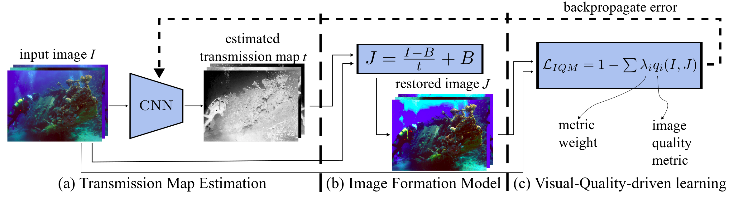
Fig. 1: Diagram of our two-stage learning. First, we fine-tune the CNN using ground-truth transmission maps, applying the mean squared error loss in the training process. Second, we take the model and adapt it by including the image restoration process (b). Finally, we perform new training in the network minimizing a loss function based on image quality metrics.

More recently, learning techniques have shown promising results when used for enhancing the visual quality of images taken from participating media [11, 12, 13, 14]. Li et al. [13] proposed a method to generate synthetic underwater images from regular air ones. They used a generative adversarial network (GAN) to simulate the water attenuation and perform the image transformation. The major drawback of their method is the requirement of a large dataset covering many different situations for a useful generalization. Ren et al. [12] estimate the transmission map using two convolutional networks. While one network extracts a general, but a rough version of the map, the second one performs local improvements. Cai et al. [11] presented a network for terrestrial images restoration, the DehazeNet. Their goal is to remove the haze by minimizing the error between expected and estimated transmission maps, which they state it is the key to recover a clean scene. Applying their approach in out of water images achieve impressive results but do not generalize to underwater scenes.

Unlike the methods mentioned above, our approach does not rely on a large dataset. Our premise is based and assessed by image quality metrics. This assumption allows us to obtain results that are directly related to the human sense of quality considering the conditions of underwater images.

2 Methodology

Our methodology comprises two-phase learning. Initially, we perform a supervised training by fine-tuning the DehazeNet [11] to estimate the transmission map. Then, we restore the input image according to an image formation model. In the second phase, we minimize a loss function composed of quality metrics to perform image restoration finally. Figure 1 illustrates the whole process.

Image Formation Model.

In the underwater environment, the image is a combination of the light coming directly from the objects composing the scene and light that was redirected towards the camera. In this work, we use the most commonly referenced image formation model [15, 8, 9]:

$$I(x)=J(x)t(x)+B(1-t(x)),$$ (1)

where $I$ is the observed light intensity, $J$ the scene radiance, $B$ the background light, and $t(x)=e^{-\beta d(x)}$ is the transmission map.

The transmission map $t$ gives the amount of light not attenuated, due to scattering or absorption, on a given point $x$ at a distance $d(x)$. The parameter $\beta$ represents the medium attenuation coefficient. Thus, $J$ can be estimated by reformulating Equation 1 as

$$J(x)=(I(x)-B)t(x)^{-1}+B.$$ (2)

Thereby, we only need to estimate $t$ and $B$ to restore an image in the underwater environment. The transmission map $t$ can be estimated using the DehazeNet. Following the prior of Drews et al. [8], we can roughly estimate the background light as being the pixel in the degraded image $I$ whose transmission map value is the highest, limited by a constant $t_{0}$, i.e., ${B=\max_{y\in\{x|t(x)\leq t_{0}\}}I(y)}$. The value $t_{0}$ is chosen as the $0.1\%$ highest pixel.

Transmission map estimation.

To adjust the network to our purpose, we proposed to perform supervised training following the guidelines of Cai et al. [11]. It consists in using underwater images as input to the network and comparing its estimated transmission map to the ground-truth maps. The loss function used in this stage is the mean squared error (MSE), defined as

$$\mathcal{L}_{t}(I,J)=\frac{1}{n}\sum_{x=1}^{n}\left(t_{I}(x)-t_{J}(x)\right)^{2},$$ (3)

where $n$ is the number of pixels, $t_{J}$ the estimated transmission map and $t_{I}$ the ground-truth.

Visual-quality-driven learning.

To overcome the absence of ground truth data for underwater scenes, we present an approach that assesses the result by computing a set of Image Quality Metrics (IQM). The IQM set $\mathcal{X}$ yields a multi-objective function that measures the enhancement of four features in the restored image in comparison to the input image. The multi-objective function is given by

$$IQM(I,J)=\sum_{X\in\mathcal{X}}\lambda_{X}q_{X}(I,J),$$ (4)

where $\lambda_{X}$ is the weight for a feature gain $q_{X}$.

We choose four metrics that are well correlated to the human visual perception to compose our IQM set: contrast, acutance, border integrity, and gray world prior.

• Contrast level: Underwater images tend to have low contrast as the amount of water between objects and the camera increases. We compute the contrast gain of a restored image $J$ over the degraded $I$ as

  $$q_{C}(I,J)=\frac{1}{n}\sum_{x=1}^{n}\left(C(J,x)^{2}-C(I,x)^{2}\right),$$ (5)

  where $C(I,x)$ is the contrast of the pixel $x$ in the gray image $I$ [7].

• Acutance: The restoration process should also enhance the acutance metric, which measures the human perception of sharpness. The restoration gain for acutance is given by

  $$q_{A}(I,J)=A(J)-A(I),$$ (6)

  where $A(I)=\frac{1}{n}\sum_{x=1}^{n}G(I,x)$ is the acutance of an image $I$. $G(I,x)$ is the gradient strength computed by applying the Sobel operator of $I$ at pixel $x$.

• Border integrity: It measures the visibility of the borders after the restoration. This measurement allows us to check how much the border increased in regions that were likely to have borders, avoiding random noise to appear in the restored image. It is calculated by

  $$q_{BI}(I,J)=\frac{\sum_{x=1}^{n}\left(E(J,x)\times E_{d}(I,x)\right)}{\sum_{x=1}^{n}E_{d}(I,x)},$$ (7)

  where $E$ is an edge detector and $E_{d}$ is the border image dilated by $5$ pixels.

• Gray world prior: The fourth feature is the gray world prior [16], a hypothesis that, under natural circumstances, the mean color of an image tends to gray. Therefore, we evaluate how distant from the gray world our restored image is by computing

  $$q_{G}(J)=(I_{max}-I_{min})-\frac{2}{n}\sum_{x=1}^{n}(I(x)-I_{m})^{2},$$ (8)

  where $I_{max}$ and $I_{min}$ are the maximum and minimum intensity a pixel can have and $I_{m}=(I_{min}+I_{max})/2$. The first term of $q_{G}$ makes the metric higher as the distance from the gray world is smaller.

After computing the gain in each quality metric, we minimize the subsequent IQM loss:

$$\mathcal{L}_{IQM}=1-IQM(I,J).$$ (9)

The weights of the network are updated by propagating the IQM error backward. Note that this step does not require labeled data. Instead of using ground truth data, our method uses the quality metrics to guide the optimization process for refining the transmission map. As a result, the final image presents a physically-plausible restoration of the input with better quality than the results achieved by other approaches.

3 Experiments

	Original	He et al.	Drews et al.	Tarel et al.	Ancuti et al.	Ours
ancuti1
ancuti2
ancuti3
galdran

Fig. 2: Four examples of images from Ancuti et al.’s dataset restored by five different approaches, including ours.

Implementation.

Our convolution network has three convolutional layers: $16$ $5{\times}5$ filters in conv1, $16$ $3{\times}3$, $5{\times}5$ and $7{\times}7$ filters in conv2, and a $6{\times}6$ filter in conv3. An element-wise maximum operation is applied to the outputs of the first layer, producing four feature maps which are concatenated and fed to the second convolutional layer. We use a max-pooling in the concatenated outputs of the second layer and a ReLU function in the last layer output. The images are normalized for values between $[0{,}1]$ after the restoration. We restricted $\sum\lambda_{X}=1$ to make the IQM score to lie in between $[0{,}1]$, where $1$ stands for the best restoration and $0$ for the worst. The values of lambdas were defined empirically, being $\lambda_{C}=0.25$, $\lambda_{A}=0.45$, $\lambda_{E}=0.05$ and $\lambda_{G}=0.25$. The weights of the network are initialized with the weights provided by Cai et al. [11]. In the initial training, we used $300$ $256{\times}256$ images from our synthetic dataset to fine-tune the network. After $1{,}500$ epochs, we switched the training from supervised to unsupervised mode and used $200$ real-scene images. We used $1{,}180$ epochs for the unsupervised training. Experimental data and source code will be publicly available.

Datasets.

For the supervised phase of our method, we create a set of synthetic underwater images using the physically based rendering engine PBRT . We render two 3D scenes and generate a total of $642$ images positioning the camera in different locations. We set the absorption and scattering coefficients according to Mobley [17]. In the unsupervised phase, we used three datasets. The first dataset is composed of $40$ images from the underwater-related scene categories of the SUN dataset  and $60$ images from Nascimento et al. [7]. In the second dataset, we used a water tank of $126$cm$\times 189$cm$\times 42$cm dimension with $665$ liters and $3$ configuration of green-tea solutions (pure water, $80$g, and $160$g of tea) to simulate distinct levels of turbidity. We selected $70$ images from a set of $695$ with the camera in different positions and different turbidity levels. The third dataset comprises a subset of images often used by the community and available in the work of Ancuti et al. [18]. Although we did not use this third dataset in training, we used it to compare our approach against other methods.

Baselines and evaluation metric.

We compared our results against four different techniques: i) DCP, which estimates the depth map of the scene by taking the dark channel; ii) UDCP, a DCP-like prior that does not take into account the red channel when computing the dark channel; iii) Tarel et al. [19] that use median filtering to restore the image; and iv) Ancuti et al. [18], which restore the image by executing a multi-scale fusion process combining four estimated weight maps. For comparison, we used the UCIQE metric proposed by Yang and Sowmya [1]. Yang and Sowmya showed that the UCIQE is in accordance with the human visual assessment. Statistics of chroma, contrast, and saturation are measures correlative to underwater image quality. The UCIQE value is given by

$$UCIQE=c_{1}\times\sigma_{c}+c_{2}\times con_{l}+c_{3}\times\mu_{s},$$ (10)

where $\sigma_{c}$ is the standard deviation of chroma, $con_{l}$ is the contrast of luminance, $\mu_{s}$ is the average of saturation, and $c_{1}=0.4680$, $c_{2}=0.2745$, $c_{3}=0.2576$.

Another metric used in our evaluation is border integrity (Equation 7 in Section 2). It assumes that the restoration process should not degenerate the most relevant borders of a degraded image. At the same time, it should preserve edges continuity. Thus, such metric tells us the gain in border conservation after a recovering process.

Results and discussion.

Table 1 shows the final result of the edge conservation. Our method outperformed all methods (zero value indicates no improvement). Figure 2 shows some visual comparison between the results achieved by all techniques. Analyzing the images ancuti3 and galdran, aside from our restoration, all others resulted in images that present a certain blur level across all the edges of the image. These results confirm that our technique tends to preserve the valid edges. It also recovers information not much visible before.

Table 2 shows the UCIQE scores . When comparing the restorations using UCIQE metric, one can see that some methods perform better in different images, but our method is the only that presents the best result for more than one image.

Table 1: Edges conservation (larger is better).

Scene	He	Drews	Ancuti	Ours
ancuti1	0.0000	0.0000	0.0003	0.0855
ancuti2	0.0000	0.0000	0.0006	0.0192
ancuti3	0.0000	0.0000	0.0008	0.0009
galdran	0.0004	0.0011	0.0062	0.0280

Table 2: Visual quality using UCIQE metric (larger is better).

Scene	Original	He	Tarel	Drews	Ancuti	Ours
ancuti1	0.8366	1.8894	0.5132	2.7105	1.8259	0.5359
ancuti2	0.4490	1.2412	0.4546	0.9285	1.1200	0.5497
ancuti3	0.7487	0.9458	0.5766	1.0913	1.0264	4.0781
galdran	0.9045	4.7779	0.5776	1.4077	4.0371	6.9439

4 Conclusion

In this paper, we presented a methodology to restore the visual quality of underwater images. Our approach uses a set of image quality metrics to guide the learning process. It consists of a deep learning model that receives an underwater image and outputs a transmission map. This map is used to obtain a set of properties from the scene. The image formation model is then used to recover the underwater scene visual information. The experiments showed that our method improves the visual quality of underwater images by not degrading their edges and also performed well on the UCIQE metric.

Acknowledgments.

The authors would like to thank CAPES, CNPq, and FAPEMIG for funding this work.

References

- [1] Miao Yang and Arcot Sowmya, “An underwater color image quality evaluation metric,” IEEE Transactions on Image Processing, vol. 24, no. 12, pp. 6062–6071, 2015.
- [2] Stéphane Bazeille, Isabelle Quidu, and Luc Jaulin, “Automatic underwater image pre-processing,” in in Proceedings of the Caracterisation du Milieu Marin (CMM’06), 2006.
- [3] Ke Gu, Guangtao Zhai, Weisi Lin, and Min Liu, “The analysis of image contrast: From quality assessment to automatic enhancement,” IEEE Transactions on Cybernetics, vol. 46, no. 1, pp. 284–297, 2016.
- [4] Lintao Zheng, Hengliang Shi, and Shibao Sun, “Underwater image enhancement algorithm based on clahe and usm,” in Information and Automation (ICIA), 2016 IEEE International Conference on, 2016, pp. 585–590.
- [5] Emanuele Trucco and Adriana T. Olmos-Antillon, “Self-tuning underwater image restoration,” IEEE Journal of Oceanic Engineering, vol. 31, no. 2, pp. 511–519, 2006.
- [6] Ran Kaftory, Yoav Y. Schechner, and Yehoshua Y. Zeevi, “Variational distance-dependent image restoration,” in Computer Vision and Pattern Recognition (CVPR), 2007 IEEE Conference on, 2007, pp. 1–8.
- [7] Erickson Nascimento, Mario Campos, and Wagner Barros, “Stereo based structure recovery of underwater scenes from automatically restored images,” in Computer Graphics and Image Processing (SIBGRAPI), 2009 XXII Brazilian Symposium on, 2009, pp. 330–337.
- [8] Kaiming He, Jian Sun, and Xiaoou Tang, “Single image haze removal using dark channel prior,” IEEE Transactions on Pattern Analysis and Machine Intelligence (TPAMI), vol. 33, no. 12, pp. 2341–2353, 2011.
- [9] Paulo LJ Drews, Erickson R. Nascimento, Silvia SC Botelho, and Mario Fernando Montenegro Campos, “Underwater depth estimation and image restoration based on single images,” IEEE Computer Graphics and Applications (CG&A), vol. 36, no. 2, pp. 24–35, 2016.
- [10] Yan-Tsung Peng and Pamela C. Cosman, “Underwater image restoration based on image blurriness and light absorption,” IEEE Transactions on Image Processing, vol. 26, no. 4, pp. 1579–1594, 2017.
- [11] Bolun Cai, Xiangmin Xu, Kui Jia, Chunmei Qing, and Dacheng Tao, “Dehazenet: An end-to-end system for single image haze removal,” IEEE Transactions on Image Processing, vol. 25, no. 11, pp. 5187–5198, 2016.
- [12] Wenqi Ren, Si Liu, Hua Zhang, Jinshan Pan, Xiaochun Cao, and Ming-Hsuan Yang, “Single image dehazing via multi-scale convolutional neural networks,” in European Conference on Computer Vision (ECCV), 2016, pp. 154–169.
- [13] Jie Li, Katherine A. Skinner, Ryan M. Eustice, and Matthew Johnson-Roberson, “Watergan: unsupervised generative network to enable real-time color correction of monocular underwater images,” IEEE Robotics and Automation Letters, vol. 3, no. 1, pp. 387–394, 2018.
- [14] Risheng Liu, Xin Fan, Minjun Hou, Zhiying Jiang, Zhongxuan Luo, and Lei Zhang, “Learning aggregated transmission propagation networks for haze removal and beyond,” arXiv preprint arXiv:1711.06787, 2017.
- [15] Raanan Fattal, “Single image dehazing,” ACM Transactions on Graphics (TOG), vol. 27, no. 3, pp. 72, 2008.
- [16] Gershon Buchsbaum, “A spatial processor model for object colour perception,” Journal of the Franklin institute, vol. 310, no. 1, pp. 1–26, 1980.
- [17] Curtis D. Mobley, Light and water: radiative transfer in natural waters, Academic press, 1994.
- [18] Cosmin Ancuti, Codruta Orniana Ancuti, Tom Haber, and Philippe Bekaert, “Enhancing underwater images and videos by fusion,” in Computer Vision and Pattern Recognition (CVPR), 2012 IEEE Conference on, 2012, pp. 81–88.
- [19] Jean-Philippe Tarel and Nicolas Hautiere, “Fast visibility restoration from a single color or gray level image,” in Computer Vision, 2009 IEEE 12th International Conference on, 2009, pp. 2201–2208.