Distributed Chernoff Test:
Optimal Decision Systems over Networks

Abstract

We study “active” decision making over sensor networks where the sensors’ sequential probing actions are actively chosen by continuously learning from past observations. We consider two network settings: with and without central coordination. In the first case, the network nodes interact with each other through a central entity, which plays the role of a fusion center. In the second case, the network nodes interact in a fully distributed fashion. In both of these scenarios, we propose sequential and adaptive hypothesis tests extending the classic Chernoff test. We compare the performance of the proposed tests to the optimal sequential test. In the presence of a fusion center, our test achieves the same asymptotic optimality of the Chernoff test, minimizing the risk, expressed by the expected cost required to reach a decision plus the expected cost of making a wrong decision, when the observation cost per unit time tends to zero. The test is also asymptotically optimal in the higher moments of the time required to reach a decision. Additionally, the test is parsimonious in terms of communications, and the expected number of channel uses per network node tends to a small constant. In the distributed setup, our test achieves the same asymptotic optimality of Chernoff’s test, up to a multiplicative constant in terms of both risk and the higher moments of the decision time. Additionally, the test is parsimonious in terms of communications in comparison to state-of-the-art schemes proposed in the literature. The analysis of these tests is also extended to account for message quantization and communication over channels with random erasures.

I Introduction

With the boom in the Internet of Things, sensor-network based solutions for inference systems have become increasingly popular [3, 4, 5]. This is mainly due to the decreasing cost of the sensors, their increasing computational capabilities, the availability of high-speed communication channels, and the redundancy provided by the distributed nature of the network [6]. Inference systems have two key functionalities: decision making (viz. hypothesis testing) and estimation. We focus on designing optimal tests for sensor networks in decision-making scenarios where the sensors actively choose their probing actions by continuously learning from past observations. Applications that fall in this framework include intrusion and target detection, and object classification and recognition [7, 8, 9, 10, 11].

Previous studies are broadly classified into two categories: fusion-center based and distributed setting. In the first case, all the nodes of the network are connected to a fusion center — and two operative modalities are considered. In the first modality, the network nodes simply deliver their observations to the fusion center, where the inference task is performed. In the second modality, the nodes exploit their computational capability to perform preliminary processing of the observations, and only a limited amount of information is delivered to the fusion center for making the final decision. This reduces the communication overhead, but may also result in a loss of performance. In the distributed setup, network nodes are connected to each other via communication links, typically forming a sparse network, and there is no central processing unit. Thus, to perform an inference task, the network nodes need to perform computations locally, share their processed data with neighboring nodes, and collectively reach a decision. A natural question in both settings is what kind of local processing to perform at the nodes, and what fusion scheme to adopt at the fusion center or at the network nodes, in order to reduce the communication burden while keeping a high level of performance. In this work, we address this question and propose statistical tests for both settings.

Hypothesis tests can be broadly classified as sequential or non-sequential tests, as well as adaptive or non-adaptive tests. In a sequential test the number of observations needed to reach a decision is not fixed in advance, but depends on the realization of the observed data. The test proceeds to collect and process data until a decision with a prescribed level of reliability can be made, and an important performance figure — in addition to the probability of correct decision — is the average number of observations required to end the test. In an adaptive test, the sensors’ probing actions are chosen on the basis of the collected data in an on-line, causal manner. Hence, the sensors learn from the past, and adapt their future probing actions in a closed-loop fashion. In this case, the sensors are said to be “active,” in the sense that measurement observations are the consequence of the sensors’ chosen probing actions. Our focus here is on sequential and adaptive tests.

We propose a Decentralized Chernoff Test (DCT) for the fusion center based setup, and a Consensus-based Chernoff Test (CCT) for the distributed setup. We provide bounds on the performance of the tests in terms of their risk, defined as the expected cost required to reach a decision plus the expected cost of making a wrong decision. We also provide converse results showing the best possible performance of any adaptive or non-adaptive sequential test over the network. We show that DCT is asymptotically optimal in terms of both the risk and the higher moments of the expected decision time, as the observation cost per unit time tends to zero. Additionally, DCT is parsimonious in terms of communication: when the observation cost per unit time tends to zero, the expected number of messages sent per node tends to a small constant. Finally, we show that CCT also retains the asymptotic optimality of Chernoff’s original solution, being order optimal up to a multiplicative constant, in terms of both risk and higher moments of decision time.

To ease the presentation, our initial analysis assumes ideal communication links carrying real-valued messages without errors. In a real network, messages are quantized into packets of a fixed length, and subject to random erasures at each transmission. In the second part of the paper, we extend our results to this scenario.

The rest of the paper is organized as follows: Section II discusses related work; Section III formulates the problem; Section IV reviews the standard Chernoff test; Section V introduces the Decentralized Chernoff Test (DCT); Section VI introduces the Consensus-based Chernoff Test (CCT); Section VII presents theoretical results on DCT and CCT; Section VIII presents simulation results; Section IX extends the analysis to quantized messages and erasure channels; Section X concludes the work. The proofs of all results appear in the Appendices.

II Related Work

Sequential tests were first introduced by Wald in 1973 [12]. One of such tests, the Sequential Probability Ratio Test (SPRT) has been proven optimal for binary hypothesis testing in [13], and for multi-hypothesis testing in [14, 15]. The performance of sequential tests can be further improved by combining them with adaptive schemes. These schemes operate in closed-loop, adapting the choice of actions to past observations. In the case of sequential and adaptive tests, Chernoff provided the optimal test for binary composite hypotheses in [16]. Its asymptotic optimality for multi-hypothesis testing was proven in [17]; see also [18] and references therein for an application. Later, the sequentiality and adaptivity gains for different classes of tests were studied, and it was established that sequential adaptive tests outperform other classes of tests [19], and that the gains can vary from application to application [20, 21, 22, 23]. All of these results were established in the case a single agent performs the test.

Different works discuss the extension to an ensemble of networked sensors independently making observations and coordinating to reach a decision [24, 25]. Different techniques for combining the information from different sensors at a fusion center are considered in  [26, 6, 27, 28]. In this case, minimization of the risk, which depends on both the decision time and the reliability of the decision, requires joint optimization over both the node level computations and the fusion center operations. Key challenges of this optimization problem are discussed in [29], and asymptotically optimal sequential (non-adaptive) tests have been developed in [30, 31].

Previous works have not considered the performance of sequential, adaptive tests in a network setting. The DCT proposed here fills this gap for star networks, namely for networks in which each node is directly connected to a fusion center. On the other hand, the CCT proposed here considers networks having a general graph structure and no central entity. In this more general case, different non-sequential tests have been developed relying on gossip protocols for distributed computation [32, 33, 34, 35, 36, 37]. These protocols can be broadly classified into two categories: consensus protocols and running-consensus protocols. In consensus protocols, a distributed computation task is performed after the collection of all the measurements at the network nodes [32, 33, 35, 36]. Necessary and sufficient conditions for convergence are well studied, see e.g., [38]. In running-consensus protocols, the collection of the measurements from the environment and the computation task are performed simultaneously at the network nodes [34, 37]. Hypothesis testing schemes typically rely on consensus over “belief vectors.” In this case, each network node holds a belief vector, whose elements represent the probability that a certain hypothesis is true, given all the information collected by the node. Different strategies are then used to transmit and combine the belief vectors over the network, leading to asymptotic learning of the correct hypothesis [39, 40, 41, 42, 43, 44]. For example, a strategy based on distributed dual averaging was proposed in [43], using an optimization algorithm from [45]. The work in [39] proposes usage of linear consensus strategies to combine the belief vectors, and [40] extends the results of [39] to the case of random time-varying networks. Other works consider Bayesian strategies for updating and combining the belief vectors at the nodes [44]. In [39, 44] the bounds on the asymptotic learning rate are presented in terms of KL-divergences of the beliefs at the different network nodes. Under the assumption that the log-likelihood ratio is bounded, finite-time analysis of the KL-divergence cost has been performed in [42]. Similar results have been obtained for networks modeled as time-varying graphs [41, 46].

Despite this huge literature, only limited attention has been given to distributed sequential hypothesis testing over general networks, which requires designing an appropriate stopping rule over the network and evaluating the corresponding expected decision time and performance in terms of risk. Recently, a sequential (non-adaptive) hypothesis test which is asymptotically optimal among non-adaptive tests has been proposed [47]. In the present work, we propose a sequential as well as adaptive hypothesis test in the distributed network setup. Unlike the previous literature, including [47], the proposed test does not perform consensus over the belief vector, and is parsimonious in terms of communication. The stopping criterion proposed in [47] is not applicable to our test. Our test is also asymptotically optimal among all adaptive or non-adaptive sequential tests, under a broad range of conditions. Finally, we point out that unlike our work, all of the above works do not consider the effect of quantization and erasures occuring over the communication links.

III Problem Formulation

Testing model

We consider an ensemble $\mathcal{L}=\{1,2,\ldots,L\}$ of sensor nodes engaged in a multi-hypothesis testing problem. The state of nature to be detected is one of $M$ exhaustive and mutually exclusive real-valued hypotheses $\{h_{i}\}_{i\in[M]}$, where $[M]=\{1,2,\dots M\}$. Nodes are connected by bi-directional communication links to form a network. At each discrete time step $n$ every node $\ell\in\mathcal{L}$ can select a probing action $u_{n,\ell}\in S$, where $S$ is a fixed set of cardinality $M$. As a consequence of this action, the node observes the realization of a real-valued random variable $Y_{n,\ell}$ whose distribution is $p_{i,\ell}^{u_{n,\ell}}$ and is known to node $\ell$ only. The node can then send one message over each of its incident links, and receive one message from each link. The probing actions and the messages sent at time $n$ can be selected based on all past observations, actions taken, and messages sent and received up to time $n-1$. It follows that the observations at each node can be dependent across time. On the other hand, given the state of nature, we assume that the observations at different nodes are conditionally independent, but not necessarily identically distributed.

Network model

We consider two network setups.

1. Star network. In this case, the network is composed of the $L$ sensors and of one special node acting as a fusion center. Each sensor is connected to the fusion center via a communication link, while there are no links between the sensors. This setup is used to introduce our Decentralized Chernoff Test (DCT).

2. General network. In this case, the network is represented by a connected graph $\mathcal{G(L,E)}$, where the edges $\{(\ell,j)\}\in\mathcal{E}$, are such that $\ell,j\in\mathcal{L}$, $\ell\neq j$. Communication and information processing tasks are fully distributed and there is no fusion center. This setup is used to introduce our Consensus-based Chernoff Test (CCT).

Communication model

We first assume an ideal communication model, where at each time step every node can send and receive a vector composed of $C$ real-values over each of its incident links. The messages sent are received instantaneously and without error. This synchronous model of communication with no queueing delay and real vector channels has been widely used in the literature of detection and estimation, see e.g. [30, 31, 32, 33, 34, 35, 36, 37, 39, 41, 42, 43, 44, 38, 47].

We then refine the communication model by taking into account that in a real packet-switched network, links can only carry a finite number of bits at each transmission, rather than real numbers. In this case, if there is a communication link connecting nodes $\ell$ and $j$, then we assume that at each time step node $\ell$ can transmit a packet of $C$ bits to node $j$ and at the same time step node $j$ can transmit a packet of $C$ bits to node $\ell$. This accounts for quantization of the real data in the previous model. In information-theoretic terms, every link behaves in each direction as a noiseless channel of finite capacity $C$ bits/transmission. As in the previous model, every packet transmission occurs synchronously in one time step, and there is no queuing delay. Although less popular than the previous one, this refined model has been considered in the context of quantized consensus in [48], and in the context of estimation and detection in [30, 31, 49, 50, 6, 51].

Finally, we further extend the communication model by considering random packet erasures. We assume that at any time step any link in the network can fail independently with probability $\epsilon$. When a link fails, packets travelling on both directions of the link are received as “erasures.” In information-theoretic terms, every link behaves in this case in both directions as a $C$-bit erasure channel without feedback, having capacity $(1-\epsilon)C$ bits/transmission. As in the previous case, transmissions are synchronous, and there is no queuing delay. A related model, where links can fail at random times but carry real numbers rather than quantized packets has been used to study consensus in [52] and estimation and detection in [53, 54, 55, 42, 56, 57, 58, 59, 60, 61].

Performance measure

Our objective is to design a scheme to select at each step the nodes’ probing actions and the messages to transmit, to eventually decide the state of nature with sufficiently high reliability. To quantify the performance of the proposed scheme, we let $N$ be the random time at which all the nodes have reached the same decision and halt the test. We consider both the expectation and the higher moments of this stopping time. Following [16], we also consider the risk, expressed as the sum of the expected cost required to reach a decision and the expected cost of making a wrong decision. Namely, under the true hypothesis $H^{*}=h_{i}$, we let the risk $\mathbb{R}_{i}^{\delta}$ of a test $\delta$ be

$$\mathbb{R}_{i}^{\delta}=c\,\mathbb{E}^{\delta}_{i}[N]+\omega_{i}\,{\mathbb{P}}_{i}^{\delta}(\hat{H}\neq h_{i}),$$ (1)

where $c$ is the observation cost per unit time, $\hat{H}$ is the final decision, $\mathbb{E}_{i}$ and $\mathbb{P}_{i}$ are the expectation and the probability operators computed under $H^{*}=h_{i}$, and $\omega_{i}$ is the cost of a wrong decision. As in [16], we evaluate the risk for all $i\in[M]$, as $c\rightarrow 0$.

Additional notation

All logarithms are to base $e$, unless otherwise indicated. For the general network case, we denote by $d^{\mathcal{G}}$ the diameter of the network, which is the maximum shortest hop-distance between any pair of nodes of $\mathcal{G(L,E)}$. We denote by $h^{\mathcal{G}}$ the shortest height of all possible spanning trees of $\mathcal{G(L,E)}$. Since the network is connected, $d^{\mathcal{G}}$ and $h^{\mathcal{G}}$ are both finite. For all $\ell\in[L]$, $u\in S$ and $i,j\in[M]$, the KL-divergence between hypotheses $h_{i}$ and $h_{j}$ is denoted by $D(p_{i,\ell}^{u}||p_{j,\ell}^{u})$, and is assumed to be finite over the entire action set $S$. We also assume that for all $\ell\in[L]$ and $i,j\in[M]$, there exists an action $u\in S$ such that $D(p_{i,\ell}^{u}||p_{j,\ell}^{u})>0$. This assumption entails little loss of generality, rules out trivialities, and is commonly adopted in the literature, see e.g., [16]. For all $\ell\in[L]$, $u\in S$ and $i,j\in[M]$, we also assume $\mathbb{E}[\log(p_{i,\ell}^{u}(Y))/\log(p_{j,\ell}^{u}(Y))]^{2}<\infty$. If $v_{1}=[v_{1,1},\ldots v_{k,1}]$ and $v_{2}=[v_{1,2},\ldots v_{k,2}]$ are two vectors of same dimension, then with $v_{1}\preceq v_{2}$ we mean that for all $i\in[k]$, $v_{i,1}\leq v_{i,2}$. Finally, we indicate with $|v_{1}|$ the vector of absolute values of the entries of $v_{1}$.

IV Standard Chernoff Test

We start by describing the Standard Chernoff Test (SCT) for a single sensor $\ell$ attempting to detect the true hypothesis $H^{*}$, having no interactions with other sensors in the network [16]. For all $n>1$ we let $y^{n}_{\ell}$ $=$ $\{y_{1,\ell},\ldots,y_{n-1,\ell}\}$, where $y_{i,\ell}$ denotes the realization of the observation collected at time step $i$, and let $u^{n}_{\ell}=\{u_{1,\ell},\ldots,u_{n-1,\ell}\}$, where $u_{i,\ell}$ denotes the realization of the action made at step $i$. For $n=1$ we initialize the set of previous actions $u^{n}_{\ell}=\emptyset$ and previous observations $y^{n}_{\ell}=\emptyset$, and let all posterior probabilities be the same, namely $\mathbb{P}(H^{*}=h_{i}|y^{n}_{\ell},u^{n}_{\ell})=1/M$.

At every step $n\geq 1$, the test proceeds as follows:

• A temporary decision is made, based on the maximum posterior probability of the hypotheses, given the past observations and actions of the sensor. Ties are resolved at random. This temporary decision is in favor of $h_{i^{*}_{n}}$ if

  $$i^{*}_{n}=\operatorname*{arg\,max}_{i\in[M]}\mathbb{P}(H^{*}=h_{i}|y^{n}_{\ell},u^{n}_{\ell}).$$ (2)

• A new action $u_{n,\ell}$ is randomly chosen among the elements of the action set $S$, according to the Probability Mass Function (PMF)

  $$Q_{i^{*}_{n}}^{\ell}=\operatorname*{arg\,max}_{q\in\mathcal{Q}}\min_{j\in M_{i^{*}_{n}}}\sum_{u{\in[M]}}q(u)D(p^{u}_{i^{*}_{n},\ell}||p_{j,\ell}^{u}),$$ (3)

  where ${\cal Q}$ denotes the set of all the possible PMFs over the $[M]$ actions, and $M_{i^{*}_{n}}=[M]\setminus\{i^{*}_{n}\}$.

• As a consequence of this action, a new observation $y_{n,\ell}$ is collected, and for all $i\in[M]$ the posterior probabilities $\mathbb{P}(H^{*}=h_{i}|y^{n+1}_{\ell},u^{n+1}_{\ell})$ are updated.

• The test stops if the worst case log-likelihood ratio crosses a prescribed fixed threshold $\gamma$, namely if

  $$\log\frac{\mathbb{P}(H^{*}=h_{i^{*}_{n},}|y^{n+1}_{\ell},u^{n+1}_{\ell})}{\max_{j\neq i^{*}_{n}}\mathbb{P}(H^{*}=h_{j}|y^{n+1}_{\ell},u^{n+1}_{\ell})}\geq\gamma,$$ (4)

  If the test stops, then the final decision is $h_{i^{*}_{n}}$, otherwise $n$ is incremented by one and the procedure continues from 1).

V Decentralized Chernoff Test

We now extend the SCT to a DCT in the star network configuration. We start by noticing that in the SCT the quantity

$$v_{i,\ell}=\max_{q\in\mathcal{Q}}\min_{j\neq i}\sum_{u{\in[M]}}q(u)D(p^{u}_{i,\ell}||p_{j,\ell}^{u})$$ (5)

is a measure of the capability of node $\ell$ to detect hypothesis $h_{i}$ (see [16] for a discussion), and plays a critical role for the selection of the action in (3) that is performed at each step and is adapted to the current belief. In a network setting, the quantity

$$I(i)=\sum_{\ell=1}^{L}v_{i,\ell}$$ (6)

represents a measure of the cumulative capability of the network to detect hypothesis $h_{i}$ and can be used for the selection of the threshold of each node in a coordinated fashion to optimize the expected decision time. Accordingly, in DCT, the fusion center collects $v_{i,\ell}$ for all $i\in[M]$ and $\ell\in[L]$, computes $I(i)$ for all $i\in[M]$, and distributes this result to all the nodes to enable their threshold selection. The nodes then perform SCTs in parallel, until they all reach the same decision and terminate the test. The three phases of the test are as follows:

Initialization phase

1. Without performing any probing action, each node $\ell$ sends the vector $v_{\ell}=[v_{1,\ell},\dots,v_{M,\ell}]$ to the fusion center.

2. The fusion center sends back to each node the cumulative capability vector $I=[I(1),\dots,I(M)]$ and, upon reception, each node $\ell$ computes the vector $\rho_{\ell}=[\rho_{1,\ell},\dots,\rho_{M,\ell}]$, representing its fraction of network capability, namely for all $i\in[M]$, we have

   $$\rho_{i,\ell}={v_{i,\ell}}/{I(i)}.$$ (7)

Test phase

Proceeding in parallel, every node $\ell$ performs a SCT using the threshold

$$\gamma=\rho_{i^{*}_{n},\ell}\,\lvert\log c\rvert.$$ (8)

This threshold depends on both the current estimate of the hypothesis and the node identity, while it was a constant in (4). If the log-likelihood ratio in (4) exceeds the threshold, node $\ell$ sends its preference for $h_{i^{*}_{n}}$ to the fusion center and continues to run the test. Hence, rather than using it as a stopping condition, the threshold is used here as a triggering condition for the communication of a preference by node $\ell$ to the fusion center.

Stopping phase

When the preferences expressed by all the nodes are the same, the fusion center sends a halting message to all the nodes, who stop the test and declare the final decision.

The proposed DCT only requires the communication of the local preferences from the nodes during the test phase, as well the the messages in the initialization phase, and the halting message. We show below that, while maintaining the same asymptotic optimality of the Chernoff test, the oscillations in the local preferences of the nodes in the test phase vanish as $c\to 0$ and, if $C\geq M$, each sensor tends to use the channel on average at most four times: two in the initialization phase, one (on average) to communicate the local preference, and one to receive the halting message. In the case $C<M$, the test retains its asymptotic optimality, although the expected number of channel uses per node increases from four to a constant that is at most $2(M+1)$, since in this case multiple transmissions are needed to communicate each vector in the initialization phase.

V-A Informal Discussion of DCT

The key idea behind the proposed DCT is to first determine the individual capabilities of the nodes for detecting the hypotheses. These capabilities are captured by the vector $v_{\ell}$, whose $i^{th}$ element is a measure of node’s $\ell$ capability to detect the hypothesis $h_{i}$. The fusion center gathers this information, and utilizes it to control the threshold at each node through the vector $\rho_{i,\ell}$. In this context, $I(i)$ is the measure of the cumulative detection capability of the network for hypothesis $h_{i}$ and $\rho_{i,\ell}$ represents the fraction of this capability contributed by node $\ell$ for hypothesis $h_{i}$. To minimize the expected time to reach a decision, it is desirable to determine the threshold for each node $\ell$ such that all the nodes require roughly the same time to reach the triggering condition in (8). This is achieved by dividing the task of hypothesis testing among the nodes based on their speed of performing the task, so that all the nodes finish their share of the task at roughly the same time.

VI Consensus-Based Chernoff Test

We now describe a CCT in a general network setup, without a fusion center. The main idea is to generalize the DCT to a fully distributed setting. CCT employs a consensus protocol to agree on the cumulative capability of the network to detect each hypothesis, performs individual SCTs, and then employs another consensus protocol to finalize the decision. To ease the presentation of CCT, as in [39, 41, 42, 43, 44] we now assume that $C\geq M$, so that consensus can be performed by exchanging real vector messages of size $M$ at every time step. In the case $C<M$ the test proceeds along the same lines, but performing vector communications of size $M$ now requires multiple time-steps, and the test completion time must be scaled accordingly. The three phases of the test are as follows:

Initialization Phase

The nodes use a distributed protocol to compute the vector $I=[I(1),\ldots,I(M)]$. Using consensus, they compute the arithmetic mean $I/L$, and then compute $I$ using their knowledge of $L$. For all $\ell\in[L]$, we let the initial estimate for $I/L$ at every node be $\hat{I}_{\ell}^{0}=[v_{1,\ell},\ldots,v_{M,\ell}]$, which can be computed locally using (5). Then, every node $\ell$ runs the following consensus protocol by iteratively exchanging messages without performing any probing action: for $n\geq 0$

$$\hat{I}_{\ell}^{n+1}=w_{\ell,\ell}\cdot\hat{I}_{\ell}^{n}+\sum_{j\in\mathcal{N}_{\ell}}w_{\ell,j}\cdot\hat{I}_{j}^{n},$$ (9)

where $\hat{I}_{\ell}^{n}=[\hat{I}_{\ell}^{n}(1),\ldots,\hat{I}_{\ell}^{n}(M)]$ is an estimate of $I/L$ at node $\ell$ and at time $n$, $w_{\ell,j}$ is the weight assigned by node $\ell$ to the estimate received from node $j$, and $\mathcal{N}_{\ell}=\{j|\{\ell,j\}\in\mathcal{E}\}$ is the set of neighbors of node $\ell$ in $\mathcal{G(L,E)}$. We now rewrite (9) in matrix form as

$$\hat{I}^{n+1}=W\cdot\hat{I}^{n},$$ (10)

where $\hat{I}^{n}$ is an $L\times M$ matrix whose $\ell$th row is $\hat{I}_{\ell}^{n}$ and $W$ is an $L\times L$ matrix whose elements satisfy

$$0<w_{\ell,j}<1\mbox{ if }j\in\mathcal{N}_{\ell}\cup\{\ell\},\mbox{ otherwise }w_{\ell,j}=0.$$ (11)

The following theorem presents necessary and sufficient conditions for the consensus protocol (10) to converge to $I/L$ as $n\rightarrow\infty$.

Theorem 1.

[38, Theorem 1]. The consensus protocol (10) converges to $I/L$ as $n\rightarrow\infty$ if and only if

$$\textbf{{1}}_{L\times 1}^{T}\cdot W=\textbf{{1}}_{L\times 1}^{T},$$ (12)

$$W\cdot\textbf{{1}}_{L\times 1}=\textbf{{1}}_{L\times 1},$$ (13)

and

$$R\left(W-\frac{\textbf{{1}}_{L\times 1}\cdot\textbf{{1}}_{1\times L}}{L}\right)<1,$$ (14)

where $R(\cdot)$ denotes the spectral radius of a matrix, and $\textbf{{1}}_{A\times B}$ is a $A\times B$ matrix of all ones. Additionally, the rate of convergence is proportional to the spectral radius in the left-hand side of (14).

Based on the above theorem, the computation of the weights in the matrix $W$ can be formulated as a convex optimization problem minimizing the spectral radius in $\eqref{eq:SC33}$, subject to (11), (12) and (13), and can be determined using standard techniques [38]. Hence, in the following we assume that, in addition to (11), $W$ verifies the conditions stated in Theorem 1.

Although the consensus protocol converges to the correct value $I/L$ as $n\rightarrow\infty$, the initialization phase must terminate in finite time and guarantee that consensus has been reached in a suitable approximate fashion.

To characterize approximate consensus, we define a local $c$-consensus status if for all $\ell\in[L]$ and $j\in\mathcal{N}_{\ell}$, we have

$$\lvert\hat{I}^{n}_{\ell}-\hat{I}^{n}_{j}\rvert\preceq\frac{c}{L^{2}}\cdot\textbf{{1}}_{1\times M}.$$ (15)

We also define a global $c$-consensus status if for all $\ell,j\in[L]$, we have

$$\lvert\hat{I}^{n}_{\ell}-\hat{I}^{n}_{j}\rvert\preceq\frac{c}{L}\cdot\textbf{{1}}_{1\times M}.$$ (16)

Since the diameter $d^{\mathcal{G}}\leq L$, it should be clear that local $c$-consensus implies global $c$-consensus.

We employ a stopping rule for the initialization phase that guarantees global $c$-consensus as illustrated in Algorithm 1. A similar rule has been previously studied in [62]. In Algorithm 1, $r^{n}_{\ell}$ indicates the number of time steps since node $\ell$ is in local $c$-consensus, namely satisfies (15). The variable $z^{n}_{\ell}$ is responsible for the percolation of the consensus information across the network. If at any node $\ell$ we have $z^{n}_{\ell}>L+1$, then the network has reached global $c$-consensus and node $\ell$ sends a termination message $m^{(1)}=1$ to its neighbors, where the superscript indicates that this is the termination message of the initialization phase. When a node receives a termination message, it halts the protocol, it scales the final estimate by $L$, so that

$$\hat{I}^{n}_{\ell}\leftarrow L\hat{I}^{n}_{\ell},$$ (17)

and it forwards the termination message to its neighbors. It follows that all the nodes receive a termination message at most $d^{\mathcal{G}}$ time steps after the first termination message has been sent, and at the end of the initialization phase for all $\ell,j\in[L]$, we have

$$\lvert\hat{I}^{n}_{\ell}-\hat{I}^{n}_{j}\rvert\preceq c\cdot\textbf{{1}}_{1\times M}.$$ (18)

In the following phases, we let $\hat{I}_{\ell}$ denote the estimate of vector $I$ at node $\ell$ at the end of the initialization phase.

Initialize $n=0$, and for all $\ell\in[L]$, $\hat{I}_{\ell}^{n}$, $r^{n}_{\ell}=0$ and $z^{n}_{\ell}=0$ 

while True do

     For all $\ell\in[L]$, broadcast local information $\hat{I}_{\ell}^{(n)}$ and $z_{\ell}^{n}$.

     Update the local cumulative capability using (9).

     if $n\geq 1$ then

         $z^{n}_{\ell}=\min\{r^{n-1}_{\ell},\min_{j\in\mathcal{N}_{\ell}\cup\{\ell\}}z^{n-1}_{j}\}+1$

     end if

     if $z^{n}_{\ell}>L+1$ or $m^{(1)}=1$ is received then

         $\hat{I}^{n}_{\ell}\leftarrow L\hat{I}^{n}_{\ell}$

         Sensor $\ell$ broadcasts $m^{(1)}=1$ and stops updating.

         Break While;

     end if

     if $\max_{j\in\mathcal{N}_{\ell}}\lvert\hat{I}_{\ell}^{(n)}-\hat{I}_{j}^{(n)}\rvert\preceq c\cdot\textbf{{1}}_{1\times M}/L^{2}$ then

         $r^{n}_{\ell}=r^{n-1}_{\ell}+1$

     else

         $r^{n}_{\ell}=0$

     end if

     $n=n+1$ 

end while

Algorithm 1 Initialization Phase of CCT

For all $i\in[M]$ and $\ell\in[L]$, $n=0$; $\hat{H}_{\ell}^{n}=\mbox{NULL}$ 

Input: Termination message of stopping phase, i.e., $m^{(3)}$

while Final decision is not made i.e. $m^{(3)}\neq 1$ do

     For all $\ell\in[L]$, perform SCT with $\gamma=\hat{\rho}_{i^{*}_{n},\ell}\,\lvert\log c\rvert$

     If $\hat{H}_{\ell}^{n}\not=$NULL, then broadcast $\hat{H}_{\ell}^{n}$

     $n=n+1$

end while

Algorithm 2 Test Phase of CCT

For all $\ell\in[L]$, initialize $n=0$; $d_{\ell,n}=x_{\ell}^{n}=0$, $m^{(3)}=0$; 

while TRUE do

     if $m^{(3)}=1$ is received from neighbor $j$ then

         Set the final decision, i.e., $\hat{H}_{\ell}^{n}=\hat{H}_{j}^{n-1}$

         Broadcast $m^{(3)}$ and $\hat{H}_{\ell}^{n}$.

         Break;

     end if

     For all $\ell\in[L]$, update $x_{\ell}^{n}$ according to (21).

     For all $\ell\in[L]$, update $d_{\ell}^{n}$ according to (20).

     if $d_{\ell}^{N}>L+1$ then

         $m^{(3)}=1$

         For all $\ell\in[L]$, broadcast $m^{(3)}$ and $\hat{H}_{\ell}^{n}$.

     else

         For all $\ell\in[L]$, broadcast $d_{\ell}^{n}$ and $\hat{H}_{\ell}^{n}$.

     end if

     $n=n+1$

end while

Algorithm 3 Stopping Phase of CCT

Test Phase

This phase is illustrated in Algorithm 2 and begins following the termination of the initialization phase, namely after receiving $m^{(1)}=1$. Every node $\ell$ performs a SCT using the threshold

$$\gamma=\hat{\rho}_{i^{*}_{n},\ell}\,\lvert\log c\rvert,$$ (19)

where $\hat{\rho}^{n}_{i^{*}_{n},\ell}=v_{i^{*}_{n},\ell}/\hat{I}_{\ell}(i^{*}_{n})$. If the log-likelyhood in (4) exceeds the threshold, then node $\ell$ updates its local preference $\hat{H}_{\ell}^{n}$ in favor of hypothesis $h_{i^{*}_{n}}$; otherwise, it sets its local preference to NULL. Similar to DCT, the node $\ell$ communicates its preference $\hat{H}_{\ell}^{n}$, if any, to its neighbors (instead than to the fusion center) and continues to run the test. Hence, rather than using it as a stopping condition, the threshold is used here as a triggering condition for the communication of the preference by node $\ell$ to its neighbors in $\mathcal{N}_{\ell}$.

Stopping Phase

This phase is illustrated in Algorithm 3 and runs in parallel with the test phase. This phase detects if all the network nodes have reached the same preference, and in this case it halts the test. At every time step $n\geq 1$, every node $\ell\in[L]$ sends $d^{n}_{\ell}$ to its neighbors, which is defined as

$$d^{n}_{\ell}=\min\left\{\min_{j\in\mathcal{N}_{\ell}\cup\{\ell\}}d^{n-1}_{j},x^{n-1}_{\ell}\right\}+1,$$ (20)

where $d_{\ell}^{0}=0$, and

$$x^{n}_{\ell}=\begin{cases}x^{n-1}_{\ell}+1\quad\mbox{ if }\forall j\in\mathcal{N}_{\ell},\hat{H}_{\ell}^{n}=\hat{H}_{j}^{n},\hat{H}_{\ell}^{n}=\hat{H}_{\ell}^{n-1},\mbox{ and }\hat{H}_{\ell}^{n}\not=\mbox{NULL},\\ 1\qquad\quad\quad\hskip 7.0pt\mbox{if }\forall j\in\mathcal{N}_{\ell},\hat{H}_{\ell}^{n}=\hat{H}_{j}^{n},\hat{H}_{\ell}^{n}\neq\hat{H}_{\ell}^{n-1},\mbox{ and }\hat{H}_{\ell}^{n}\not=\mbox{NULL},\\ 0\qquad\quad\quad\hskip 3.0pt\mbox{ otherwise},\end{cases}$$ (21)

where $x_{\ell}^{0}=0$.

The rationale of (20) and (21) is as follows. Suppose $x^{n}_{\ell}=k$. Then, for the past $k$ time steps the local preference of the neighbors of node $\ell$ was the same as the local preference $\hat{H}_{\ell}^{n}$ of node $\ell$. The value of $d^{n}_{\ell}$ is responsible for the percolation of this information along the network. Using (21), if node $j\in\mathcal{N}_{\ell}$ does not report any local preference, then the value $x^{n}_{j}=0$ is received by the neighbors of $j$. If at any node $\ell$ we have $d^{N}_{\ell}>L+1$, then there exists a time $k\leq N$ at which the local decisions of all the nodes are the same, i.e., $\min_{j\in[L]}x_{j}^{k}\geq 1$ (see Lemma 13 in Appendix B-E). This node $\ell$ sends the final decision $\hat{H}_{\ell}^{N}$ and the termination message $m^{(3)}=1$ to its neighbors, where $m^{(3)}=1$ represents the termination message for the stopping phase. When a node receives the termination message and the final decision $\hat{H}_{\ell}^{N}$, it halts the test and forwards $m^{(3)}$ along with $\hat{H}_{\ell}^{N}$ to its neighbors. It follows that all nodes receives the termination message and the final decision at most $d^{\mathcal{G}}$ time steps after the first termination message of the stopping phase has been sent.

VI-A Informal Discussion of CCT

As in DCT, the key idea behind CCT is to first determine the individual capabilities of the nodes for detecting the hypotheses. These capabilities are captured by the vector $v_{\ell}$, whose $i^{th}$ element is a measure of node’s $\ell$ capability to detect the hypothesis $h_{i}$. However, in contrast to DCT, there is no central entity to facilitate the sharing of this information among different nodes, and a consensus algorithm is used — in the first phase of CCT — to gain global knowledge at each node of the capabilities of all the other nodes. If the consensus algorithm stops at time $N$, then $\hat{\rho}^{N}_{i,\ell}$ denotes the estimated fraction of the capability contributed by node $\ell$ for hypothesis $h_{i}$. To minimize the expected time to reach a decision, it is desirable to determine this threshold for each node $\ell$ such that all the nodes require roughly the same time to reach the triggering condition in (8). This is achieved by dividing the task of hypothesis testing among the nodes based on their speed of performing the task, so that all the nodes finish their share of the task roughly at the same time. The decision phase is a distributed stopping criterion for the Chernoff test, and ensures that the nodes stop the test as they reach the same decisions.

VII Performance analysis

We now present the performance analysis of our tests. The proofs of all theorems are deferred to the Appendices.

VII-A Lower Bounds for a Sequential and an Adaptive test

In this section, we present lower bounds on two different performance measures, namely risk and decision time, for any sequential and adaptive test. The superscript $\delta$ is appended to quantities that refer to a generic test and $N$ indicates the time required to take a decision.

Theorem 2.

(Converse) For any hypothesis testing scheme $\delta$ operating over a network as described in Section III, we have that for all $i\in[M]$, if the probability of missed detection is

$$\mathbb{P}^{\delta}_{i}(\hat{H}\neq h_{i})=O(c\,|\log c|),\;\;\mbox{ as }c\to 0,$$ (22)

then we have, for all integers $r\geq 1$,

$$\mathbb{E}^{\delta}_{i}[N^{r}] \geq \Bigg{(}(1+o(1))\frac{\lvert\log c\rvert}{I(i)}\Bigg{)}^{r},\mbox{ as }c\to 0.$$ (23)

Using (23) with $r=1$, we also have

$$\mathbb{R}_{i}^{\delta} \geq (1+o(1))\frac{c\,\lvert\log c\rvert}{I(i)},\;\;\mbox{ as }c\to 0.$$ (24)

The lower bounds provided by Theorem 2 hold for any scheme operating in our problem formulation setting, in both a star network or general network configuration. In the case the network is composed of a single node and $r=1$, they reduce to Chernoff’s original results [16].

VII-B Upper bounds for proposed DCT and CCT schemes

We now provide upper bounds on the performance of our schemes, starting with DCT. In the following theorems, the superscript ${\cal D}$ refers to the DCT. Part $(i)$ of Theorem 3 states that the probability of making a wrong decision can be made as small as desired by an appropriate choice of the observation cost $c$. Part $(ii)$ provides a bound on the expected time to reach the final decision, and part $(iii)$ bounds the risk as an immediate consequence of parts $(i)$ and $(ii)$. Finally, part $(iv)$ presents the bound on the higher moments of the decision time of DCT.

Theorem 3.

(Direct). The following statements hold:
$(i)$ For all $c\in(0,1)$ and all $i\in[M]$, the probability that DCT makes an incorrect decision is

$${\mathbb{P}}^{{\cal D}}_{i}(\hat{H}\neq h_{i})\leq\min\{(M-1)c,1\}.$$ (25)

$(ii)$ For all $\ell\in[L]$, $i,j\in[M]$ and $u\in S$, if $\mathbb{E}\big{[}\log{p_{i,\ell}^{u}(Y)}/{p_{j,\ell}^{u}(Y)}\big{]}^{2}<\infty$, then we have

$$\mathbb{E}_{i}^{{\cal D}}[N]\leq(1+o(1))\frac{\lvert\log c\rvert}{I(i)},\;\;\mbox{ as }c\to 0.$$ (26)

$(iii)$ Combining $(i)$ and $(ii)$, we have

$$\mathbb{R}_{i}^{{\cal D}}\leq(1+o(1))\frac{c\,\lvert\log c\rvert}{I(i)},\;\;\mbox{ as }c\to 0.$$ (27)

$(iv)$ For all $\ell\in[L]$, $i,j\in[M]$, $u\in S$ and all integers $r\geq 2$, if $\mathbb{E}\big{[}\lvert\log{p_{i,\ell}^{u}(Y)}/{p_{j,\ell}^{u}(Y)}\rvert^{r+1}\big{]}<\infty$, then we have

$$\mathbb{E}_{i}^{{\cal D}}[N^{r}]\leq\Bigg{(}(1+o(1))\frac{c\,\lvert\log c\rvert}{I(i)}\Bigg{)}^{r},\mbox{ as }c\to 0.$$ (28)

In the above theorem, the bound on the expected decision time in $(ii)$ requires the second moment of the log-likelihood ratio to be finite. Likewise, for all $r\geq 2$, the bound on the $r^{th}$ moment of the decision time requires the $r+1^{st}$ moment of the log-likelihood ratio to be finite.

The next result is a consequence of Theorems 2 and 3. It shows the asymptotic optimality of DCT, and presents the expected communication overhead, as $c\to 0$.

Theorem 4.

For any hypothesis testing scheme $\delta$ operating over a network as described in Section III, we have
$(i)$ For all $\ell\in[L]$, $i,j\in[M]$ and $u\in S$, if $\mathbb{E}\big{[}\log{p_{i,\ell}^{u}(Y)}/{p_{j,\ell}^{u}(Y)}\big{]}^{2}<\infty$, then we have

$$\lim_{c\to 0}\frac{\mathbb{E}_{i}^{{\cal D}}[N]}{\mathbb{E}_{i}^{{\delta}}[N]}\leq 1,\mbox{ and}$$ (29)

$$\lim_{c\to 0}\frac{\mathbb{R}_{i}^{{\cal D}}}{\mathbb{R}_{i}^{{\delta}}} \leq 1.\;\;$$ (30)

$(ii)$ For all $\ell\in[L]$, $i,j\in[M]$, $u\in S$ and all integers $r\geq 2$, if $\mathbb{E}\big{[}\lvert\log{p_{i,\ell}^{u}(Y)}/{p_{j,\ell}^{u}(Y)}\rvert^{r+1}\big{]}<\infty$, then we have

$$\lim_{c\to 0}\frac{\mathbb{E}_{i}^{{\cal D}}[N^{r}]}{\mathbb{E}_{i}^{{\delta}}[N^{r}]}\leq 1.$$ (31)

$(iii)$ Assuming $C\geq M$, and letting the communication overhead $C_{O}$ be the number of channel usages by each node, we have

$$\lim_{c\rightarrow 0}\mathbb{E}^{{\cal D}}_{i}[C_{O}]=4.$$ (32)

Combining Theorem 3 and Theorem 4, it follows that DCT is asymptotically optimal in terms of stopping time and risk, as the observation cost tends to zero. This asymptotic optimality, expressed by (29), (30), and (31), holds for all values of $C$, although in the case $C<M$ the expected number of channel uses per node in (32) increases from four to a constant that is at most $2(M+1)$, due to multiple transmissions required to communicate each vector in the initialization phase. We also point out that the performance of DCT depends only on the cumulative capability $I(i)$ of the network to detect hypothesis $h_{i}$, and is independent of how the capabilities $v_{i,\ell}$ are distributed over the network. If two networks have the same cumulative capabilities, then the minimum expected decision time will be the same for both of them. These results hold irrespective of the number of nodes in the network.

We now provide upper bounds on the performance of CCT. We make use of the following well known lemma:

Lemma 5.

[63, Proposition 1]. For any a connected graph $\mathcal{G(L,E)}$ with weights assigned to the edges satisfying (11), we have that

$$0<\eta(W^{h^{\mathcal{G}}})<1,$$

where

$$\eta(W)=\min_{i\neq j}\sum_{k=1}^{L}\min\{w_{i,k},w_{j,k}\}$$

is the ergodic coefficient of the weight matrix $W$.

In the following theorems, the superscript ${\cal C}$ refers to the CCT. Part $(i)$ of Theorem 6 states that the probability of making a wrong decision can be made as small as desired by an appropriate choice of $c$. Part $(ii)$ provides a bound on the expected time to reach the final decision, and part $(iii)$ bounds the risk as an immediate consequence of parts $(i)$ and $(ii)$. Finally, part $(iv)$ presents the bound on the higher moments of the decision time of CCT.

Theorem 6.

(Direct). Assuming $C\geq M$, the following statements hold:
$(i)$ For all $c\in(0,1)$ and all $i\in[M]$, the probability that CCT makes an incorrect decision is

$${\mathbb{P}}^{{\cal C}}_{i}(\hat{H}\neq h_{i})\leq\min\left\{(M-1)c^{\frac{1}{1+c/I(i)}},1\right\}.$$

$(ii)$ For all $\ell\in[L]$, $i,j\in[M]$ and $u\in S$, if $\mathbb{E}\big{[}\log{p_{i,\ell}^{u}(Y)}/{p_{j,\ell}^{u}(Y)}\big{]}^{2}<\infty$, then as $c\rightarrow 0$ we have

$$\begin{split}&\mathbb{E}_{i}^{{\cal C}}[N]\leq(1+o(1))\Bigg{(}\frac{h^{\mathcal{G}}\cdot|\log(c/\max_{j\in[L]}I(j))|}{|\log\big{(}1-\eta(W^{h^{\mathcal{G}}})\big{)}|}+\frac{\lvert\log c\rvert}{I(i)-c}\Bigg{)}.\end{split}$$ (33)

$(iii)$ Combining $(i)$ and $(ii)$, as $c\rightarrow 0$ we have

$$\begin{split}\mathbb{R}_{i}^{{\cal C}}&\leq(1+o(1))\Bigg{(}\frac{h^{\mathcal{G}}\cdot\lvert\log(1/\max_{j\in[L]}I(j))\rvert}{\lvert\log(1-\eta(W^{h^{\mathcal{G}}}))\rvert}+\frac{1}{I(i)-c}\Bigg{)}\cdot c\lvert\log c\rvert.\qquad\end{split}$$ (34)

$(iv)$ For all $\ell\in[L]$, $i,j\in[M]$, $u\in S$ and all integers $r\geq 2$, if $\mathbb{E}\big{[}\lvert\log{p_{i,\ell}^{u}(Y)}/{p_{j,\ell}^{u}(Y)}\rvert^{r+1}\big{]}<\infty$, then as $c\rightarrow 0$ we have

$$\mathbb{E}_{i}^{{\cal C}}[N^{r}]$$

$$\leq\Bigg{(}(1+o(1))\Bigg{(}\frac{h^{\mathcal{G}}\cdot|\log(c/\max_{j\in[L]}I(j))|}{|\log(1-\eta(W^{h^{\mathcal{G}}}))|}+\frac{\lvert\log c\rvert}{I(i)-c}\Bigg{)}\Bigg{)}^{r}.$$ (35)

The following result is a consequence of Theorems 2 and 6, and shows that CCT is asymptotically optimal, up to a constant factor, as the observation cost tends to zero.

Theorem 7.

For any hypothesis testing scheme $\delta$ operating over a network as described in Section III and assuming $C\geq M$, we have:
$(i)$ For all $\ell\in[L]$, $i,j\in[M]$ and $u\in S$, if $\mathbb{E}\big{[}\log{p_{i,\ell}^{u}(Y)}/{p_{j,\ell}^{u}(Y)}\big{]}^{2}<\infty$, then

$$\begin{split}&\lim_{c\to 0}\frac{\mathbb{E}_{i}^{{\cal C}}[N]}{\mathbb{E}_{i}^{{\delta}}[N]}\leq\Bigg{(}\frac{I(i)h^{\mathcal{G}}\cdot\lvert\log(1/\max_{j\in[L]}I(j))\rvert}{\lvert\log(1-\eta(W^{h^{\mathcal{G}}}))\rvert}+1\Bigg{)}.\;\;\end{split}$$ (36)

Additionally,

$$\lim_{c\to 0}\frac{\mathbb{R}_{i}^{{\cal C}}}{\mathbb{R}_{i}^{{\delta}}} \leq \Bigg{(}\frac{I(i)h^{\mathcal{G}}\cdot\lvert\log(1/\max_{j\in[L]}I(j))\rvert}{\lvert\log(1-\eta(W^{h^{\mathcal{G}}}))\rvert}+1\Bigg{)}.$$ (37)

$(ii)$ For all $\ell\in[L]$, $i,j\in[M]$, $u\in S$ and all integers $r\geq 2$, if $\mathbb{E}\big{[}\lvert\log{p_{i,\ell}^{u}(Y)}/{p_{j,\ell}^{u}(Y)}\rvert^{r+1}\big{]}<\infty$, then we have

$$\lim_{c\to 0}\frac{\mathbb{E}^{{\cal C}}_{i}[N^{r}]}{\mathbb{E}^{{\delta}}_{i}[N^{r}]} \leq \Bigg{(}\frac{I(i)h^{\mathcal{G}}\cdot\lvert\log(1/\max_{j\in[L]}I(j))\rvert}{\lvert\log(1-\eta(W^{h^{\mathcal{G}}}))\rvert}+1\Bigg{)}^{r}.$$ (38)

While Theorems 6 and 7 provide bounds for the case $C\geq M$, it should be clear from their proof that when $C<M$ CCT is still asymptotically optimal up to a constant factor, as $c\rightarrow 0$. In this case, the right-hand sides of (36) and (37) are simply scaled by an additional factor that is upper bounded by $M$, due to the multiple transmissions required to complete each vector transmission. Similarly, the right-hand side of (38) is scaled by a factor upper bounded by $M^{r}$.

The decision time of CCT (see (33) and (12)) depends on two terms: $A_{1}$ and $A_{2}$, where

$$A_{1}=\frac{h^{\mathcal{G}}\cdot|\log(c/\max_{j\in[L]}I(j))|}{|\log\big{(}1-\eta(W^{h^{\mathcal{G}}})\big{)}|},$$

$$A_{2}=\frac{\lvert\log c\rvert}{I(i)-c}.$$

Here, $A_{1}$ corresponds to the expected time of the initialization phase. Since this phase performs consensus over the network, this time depends on the network parameters $h^{\mathcal{G}}$ and matrix $W$. Similarly, $A_{2}$ corresponds to the expected time of the test phase, where the Chernoff test is performed independently at all the nodes. This time is independent of the network parameters. Finally, since the decision phase of CCT begins only after the termination of the initialization phase and is dependent on the test phase, the expected decision time of CCT depends on $A_{1}+A_{2}$. Thus, in Theorem 7, the ratio of the performance parameters of CCT and of the optimal test converges to the constant $1+{I(i)h^{\mathcal{G}}\cdot\lvert\log(1/\max_{j\in[L]}I(j))\rvert}/{\lvert\log(1-\eta(W^{h^{\mathcal{G}}}))\rvert}$. It follows that the gap between the CCT and the optimal test is given by ${I(i)h^{\mathcal{G}}\cdot\lvert\log(1/\max_{j\in[L]}I(j))\rvert}/{\lvert\log(1-\eta(W^{h^{\mathcal{G}}}))\rvert}$, and as the expected time of initialization phase decreases this gap decreases.

As a final remark, we point out that the star network configuration is a special case of the distributed setup. In this case, the cumulative capability vector $I$ can be estimated (with no error) in two time steps at all the nodes, i.e., for $n=2$ and $\ell,j\in[L]$, the equivalent of (16) is

$$\lvert\hat{I}^{n}_{\ell}-\hat{I}^{n}_{j}\rvert\preceq 0\cdot\textbf{{1}}_{1\times M},$$ (39)

and is independent of $c$. In the regime of vanishing cost $c\to 0$, we have that $A_{1}+A_{2}=2+A_{2}$, which implies the asymptotic optimality of DCT.

VIII Numerical Results

In this section, we evaluate the performance of both DCT and CCT by simulations, and compare the results to the theoretical bounds presented in the previous section. The performance of these tests is evaluated for different sizes of networks. In our experiments, the number of hypotheses is $M=3$. The probability distribution $p_{i,\ell}^{u}$,  $i=1,\dots,M$, is Bernoulli with parameter $p$, which is selected uniformly at random from $(0,1/3)$,$(1/3,2/3)$ and $(2/3,1)$ for $i=1,2$ and $3$ respectively.

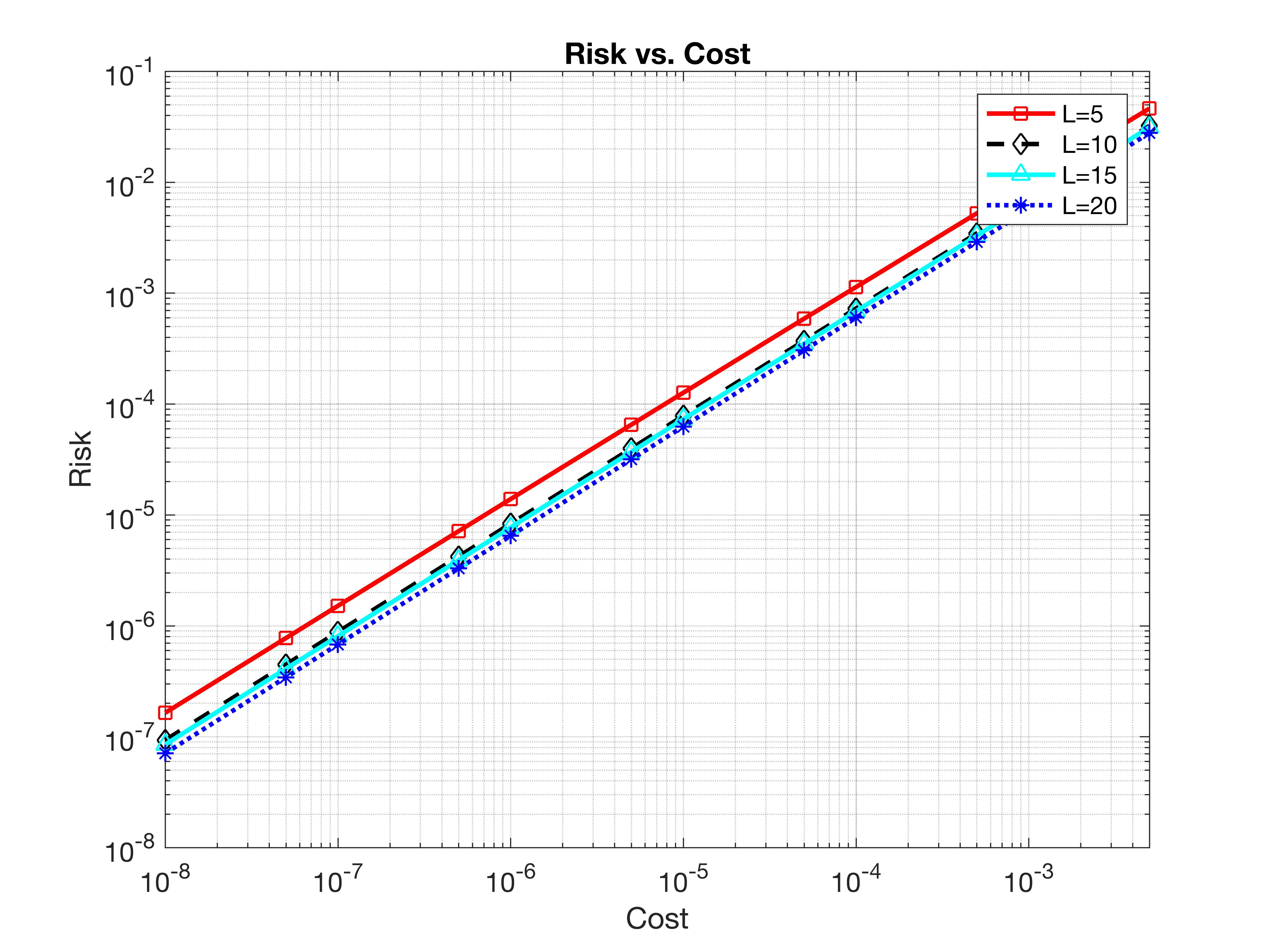
Figure 1: Performance of DCT: risk vs. cost $c$ for different number of sensors $L$

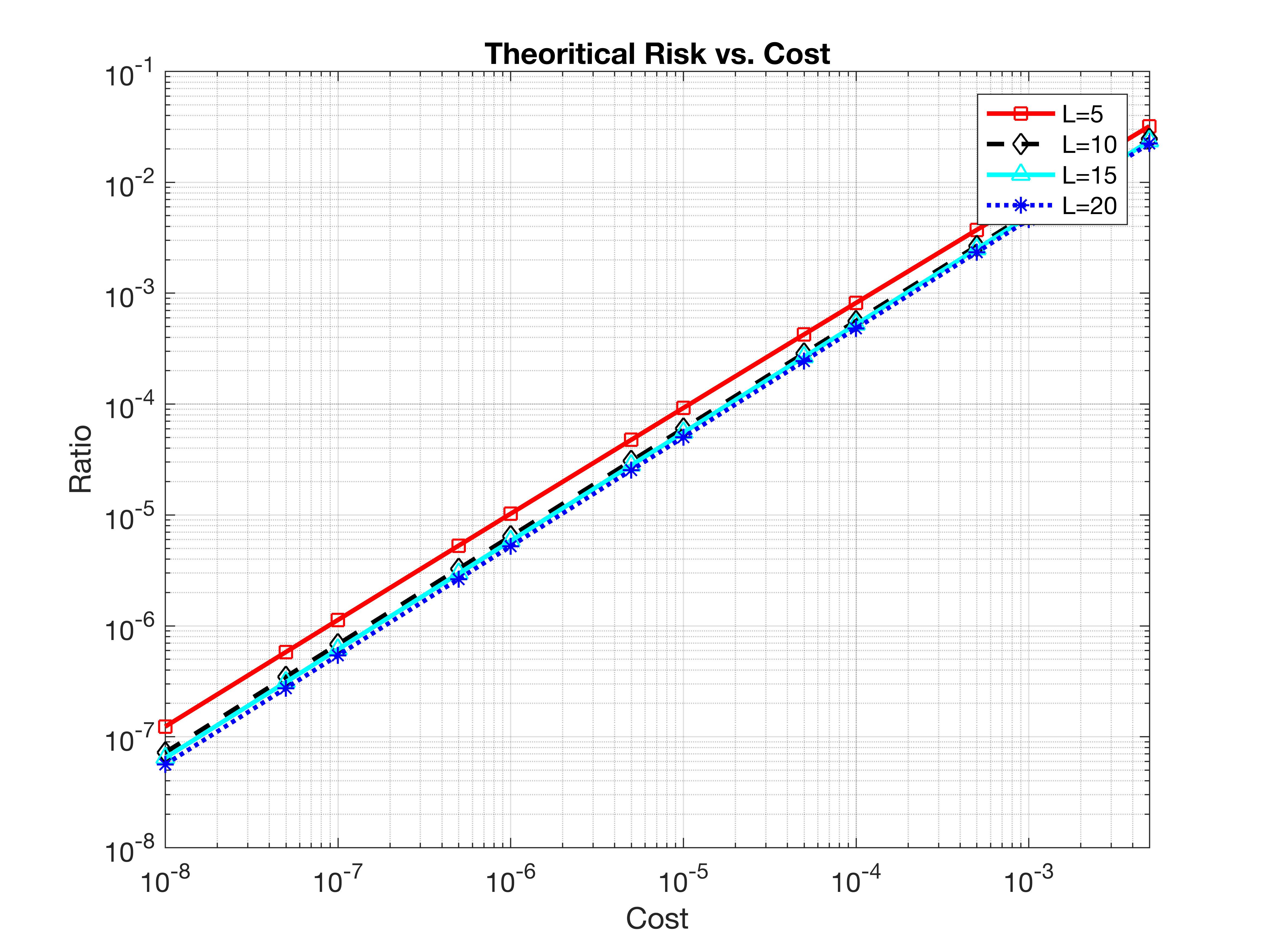
Figure 2: Performance of DCT according to Theorem 3: risk vs. cost $c$ for different number of sensors $L$

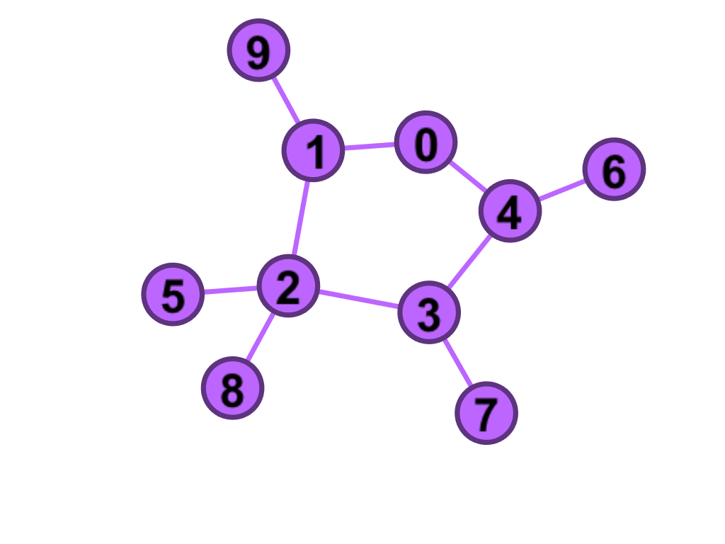
Figure 3: An example of sensor network with $L=10$ nodes.

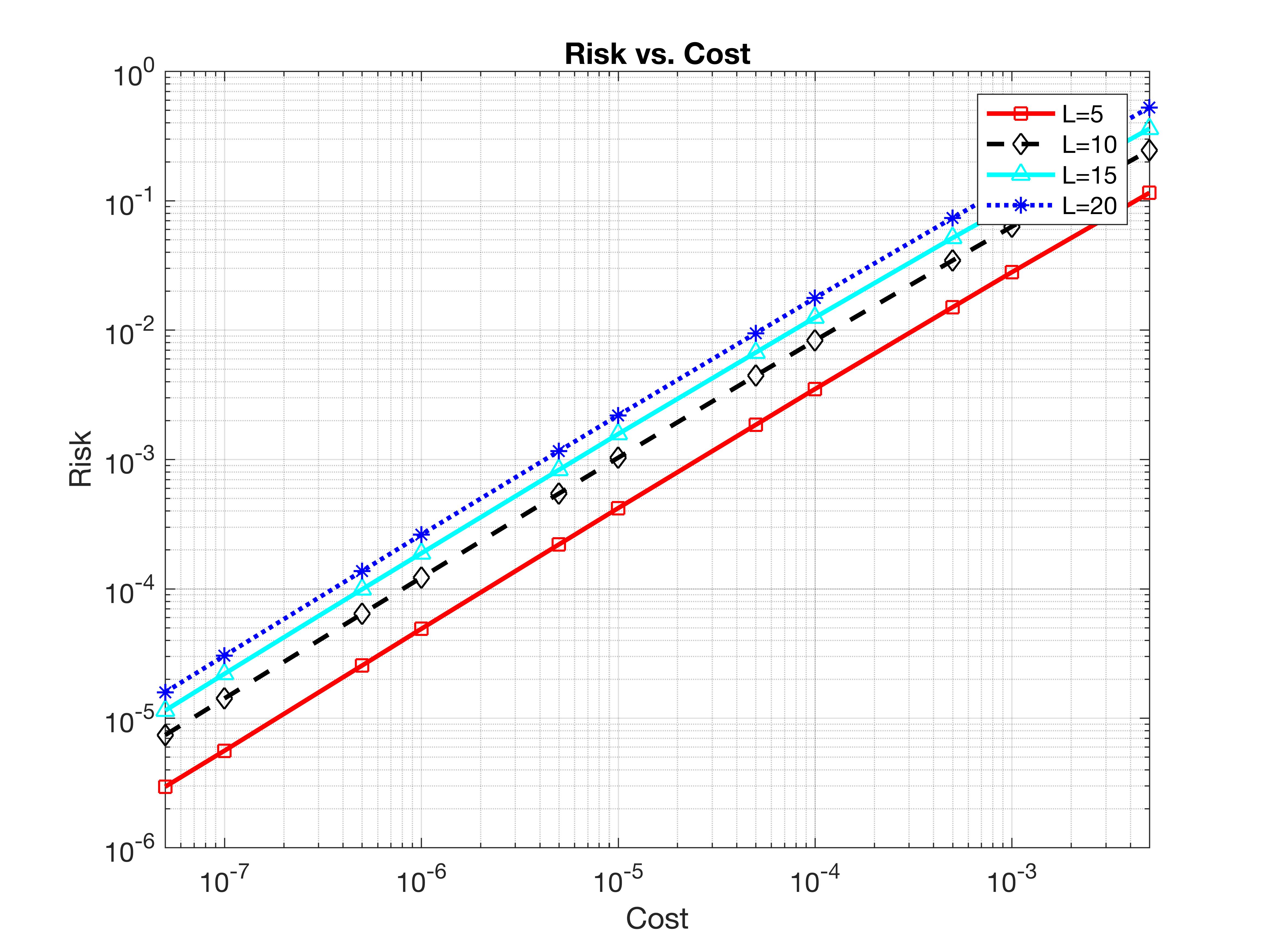
Figure 4: Performance of CCT for the ring with random attachments topology: risk vs. cost $c$ for different number of sensors $L$

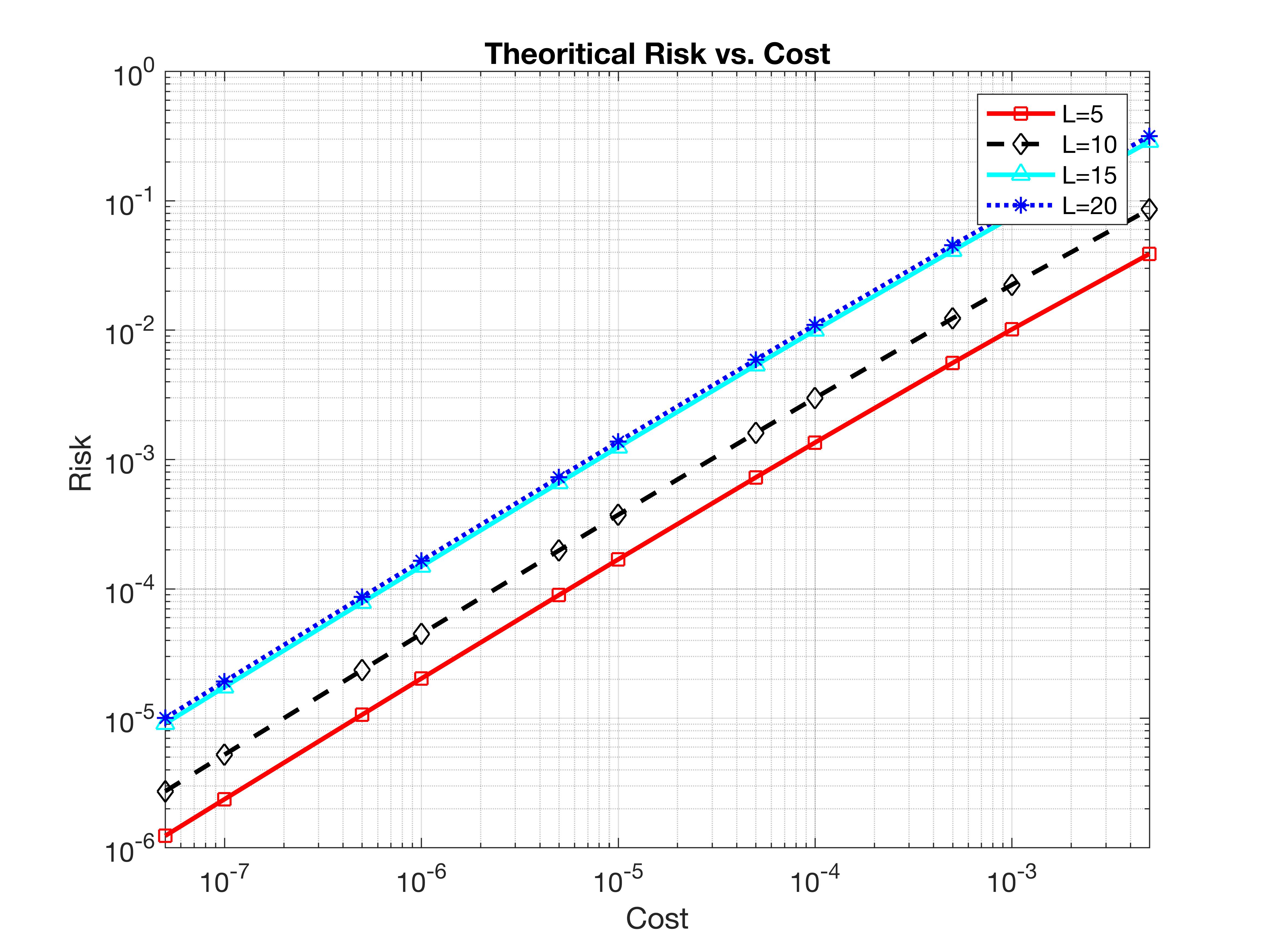
Figure 5: Performance of CCT according to Theorem 6 for the ring with random attachments topology: risk vs. cost $c$ for different number of sensors $L$

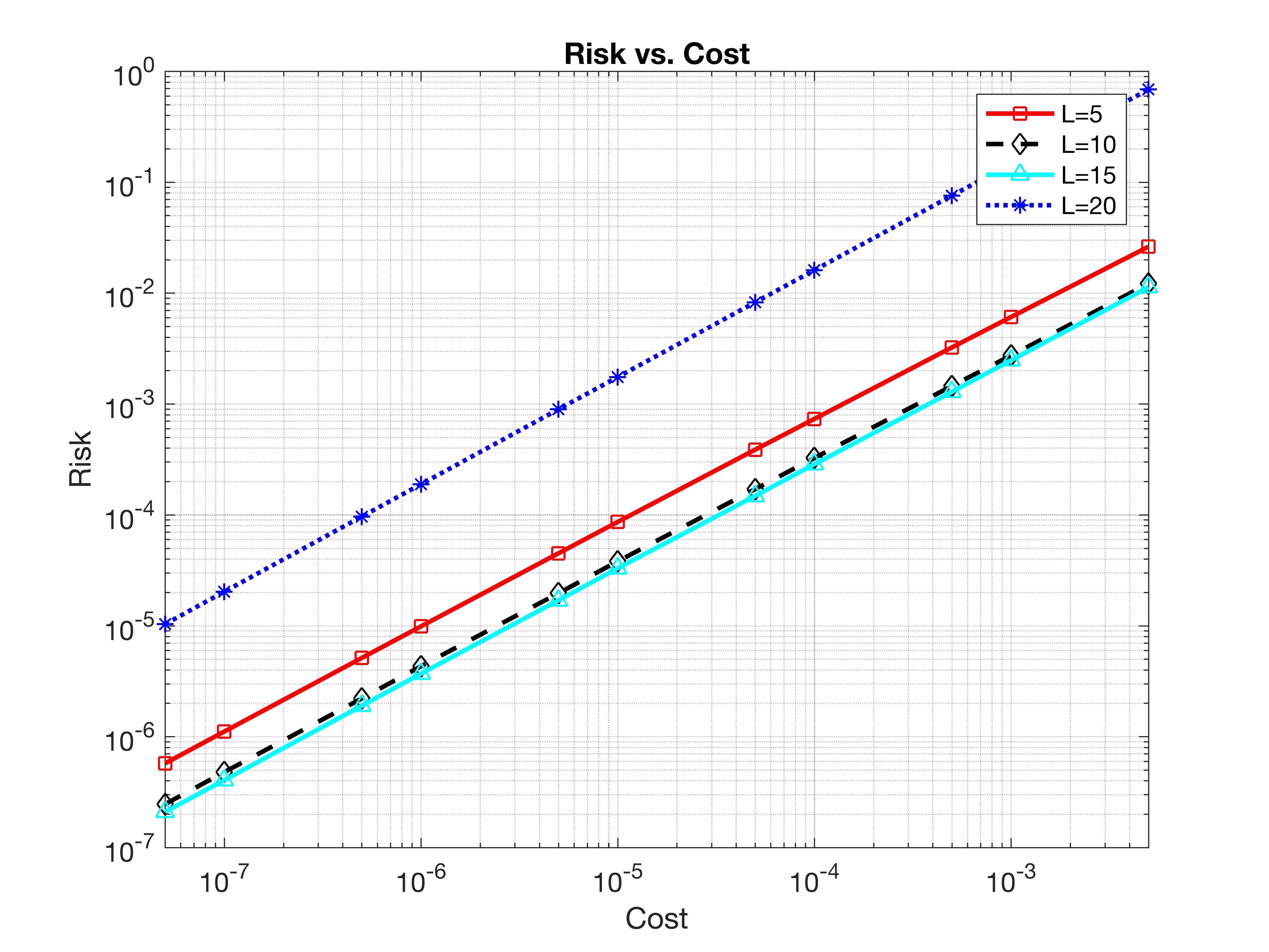
Figure 6: Performance of CCT for the tree topology: risk vs. cost $c$ for different number of sensors $L$

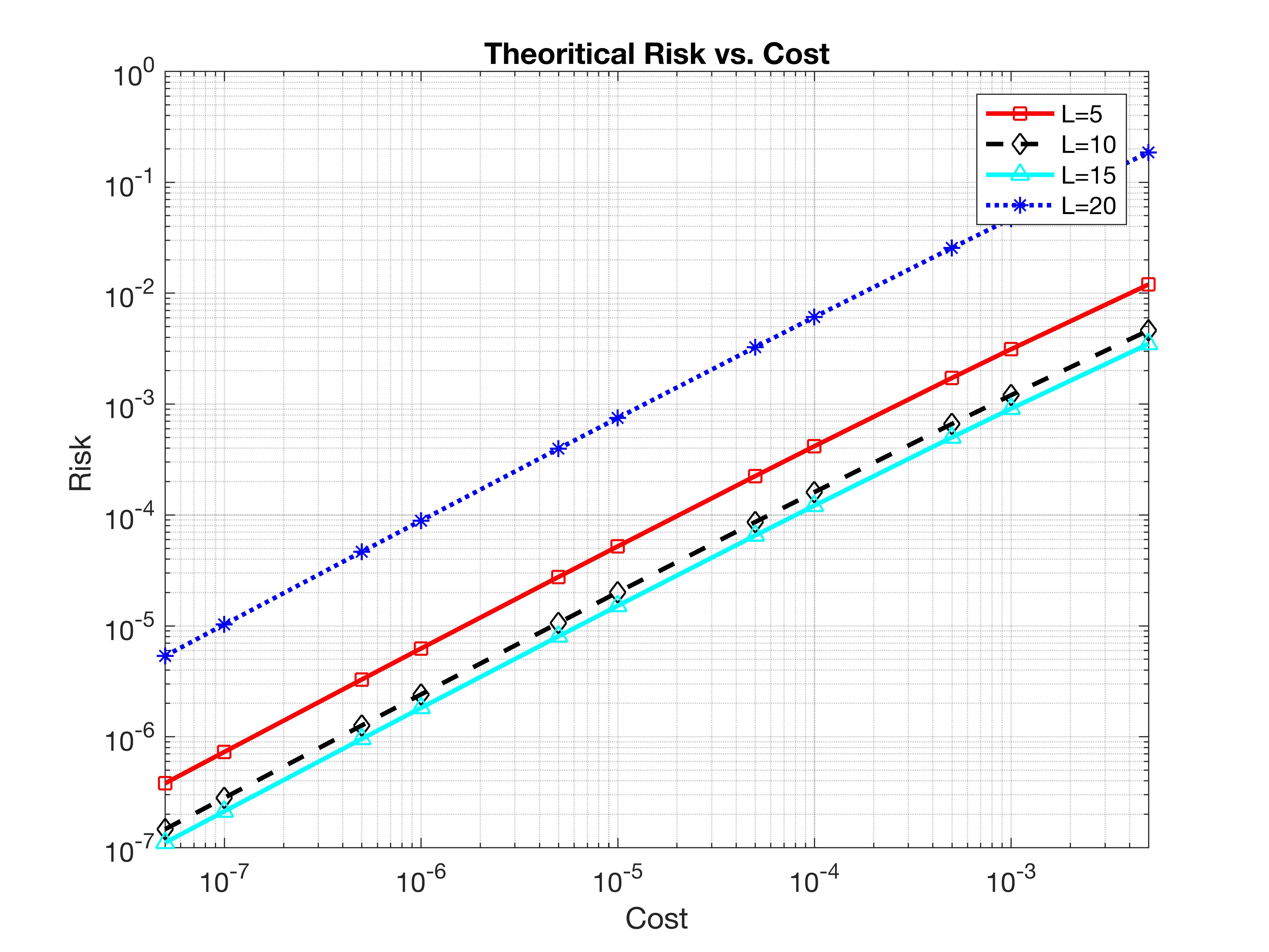
Figure 7: Performance of CCT according to Theorem 6 for the tree topology: risk vs. cost $c$ for different number of sensors $L$

Figure 2 shows the risk of DCT in a fusion center based setup, as obtained by simulations. Figure 2 shows the corresponding value of the risk, as predicted by Theorem 3. The risk decreases as the observation cost $c$ decreases. This is because the threshold in the triggering condition (8) increases, which ensures that the nodes have a greater confidence about their local decision. On the other hand, the risk decreases by increasing the number of sensors $L$, because the cumulative capability of the network to detect the hypothesis, defined in (6), increases with $L$, and the task of hypothesis testing is divided among a larger number of sensors. Hence, the final decision can be reached more quickly, and this decreases the risk. The trends are in agreement with the theoretical results obtained for DCT.

Our simulations also confirm the prediction that, on the average, only four channel usages are required, per single sensor, see (32) in Theorem 4. The results of these simulations are not reported here for the sake of brevity. We only mention that, on rare occasions, for individual realizations it may happen that the number of channel usages is substantially larger than four —a manifestation of the long-run phenomenon [64, p. 110]. In practice, this can be remedied by resorting to a truncated version of the sequential test, for which the maximum number of probing actions is fixed, see [65, 66] and references therein for a discussion, and see [67] for a simple implementation of truncation. A precise analysis of DCT using truncated tests is out of the scope of the present paper.

The performance of CCT is evaluated for two network topologies. In the first topology, given the number of network nodes $L$, $\lceil L/2\rceil$ sensors are connected to form a ring, and the remaining sensors are randomly connected to the sensors in the ring. An example of network with $L=10$ is shown in Figure 3. In this case, the spanning height of the tree is linear in $L$. In the second topology, given the number of network nodes $L$, the nodes are connected to form a binary tree. In this case, the spanning height of the tree is $\mathcal{O}(\log_{2}L)$.

Figure 5 shows the performance of CCT for the ring with random attachments, obtained by computer simulations. Figure 5 shows the value of risk according to Theorem 6. Like in the case of DCT, the risk of CCT decreases as the observation cost $c$ decreases. Instead, the behavior as function of $L$ is different. Unlike DCT, the risk of CCT increases by increasing the number of network nodes $L$. This effect can be explained by observing that in CCT there is a trade-off between the time required by the initialization phase and the time required by the test phase. For the considered network $\mathcal{G}$ and consensus matrix $W$, as the number of nodes $L$ increases, the consensus scheme in the initialization phase will require more time in comparison to the test phase. Additionally, the time required by the test phase decreases with $L$, for the same reasons as in the DCT case. Figures 5 and 5 show that the consensus between the sensors in the first phase of CCT becomes the dominating factor in the decision time. This is in agreement with the theoretical bounds provided in Theorem 6.

Figures 7 and 7 show the performance of CCT for the tree topology, via simulations and using the theoretical predictions of Theorem 6, respectively. The risk of CCT decreases as $c$ decreases. Unlike the ring topology with random attachments, the risk decreases by increasing $L$ until $L=15$, and then increases. In this setup, for the initial values of $L$, the time required by the test phase is larger than the time for the initialization phase, hence, it is the dominating factor in the decision time of CCT. On the contrary, for $L=20$, the time of the initialization phase becomes dominant, which explains why the risk increases with $L$. Finally, comparing Figures 7 and 7, we see that the theoretical values of the risk are close to the results of numerical simulations.

IX Extension to Channels with Quantized Messages and Link Failures

In the previous sections, we have assumed a communication model carrying real numbers over ideal links, without errors. This models a situation where transmission are finely quantized and adequately protected against errors. We now wish to explicitly take into account the effect of data quantization, and of link failures leading to packet erasures.

IX-A Channels with Quantized Messages

We start by considering channels supporting quantized messages, rather than real numbers, as described in Section III. We extend our previous results by describing the key changes to both DCT and CCT formulations.

IX-A1 DCT with quantized messages

In the initialization phase, the vectors $v_{\ell}$ and $I$ need to be quantized using $C$ bits before transmission. Accordingly, at the sensor nodes we construct the quantized vector $\lfloor v_{\ell}\rfloor=[\lfloor v_{1,\ell}\rfloor,\ldots,\lfloor v_{M,\ell}\rfloor]$ and at the fusion center we construct the corresponding vector $\lfloor I\rfloor=[\lfloor I(1)\rfloor,\dots,\lfloor I(M)\rfloor]$. By (6) we have that for all $i\in[M]$ and $\ell\in[L]$, $v_{i,\ell}\leq I(i)$. It follows that to construct the first vector we can divide the interval $[0,\max_{i}I(i)]$ uniformly into $Q$ sub-intervals, where $Q=2^{C/M}$, and let $\lfloor v_{i,\ell}\rfloor$ be the nearest value among the $Q$ quantization levels smaller than $v_{i\ell}$. In this way, the difference between any two contiguous quantization levels for $v_{i,\ell}$ is

$$\Delta\Big{(}\max_{i}I(i),Q\Big{)}=\frac{\max_{i}I(i)}{Q}.$$ (40)

The quantized vector $\lfloor v_{\ell}\rfloor=[\lfloor v_{1,\ell}\rfloor,\ldots,\lfloor v_{M,\ell}\rfloor]$ is then sent by each node to the fusion center using $M\cdot\log_{2}Q=C$ bits in one transmission. On the other hand, for the second vector we let, for all $i\in[M]$

$$\lfloor I(i)\rfloor=\sum_{\ell=1}^{L}\lfloor v_{i,\ell}\rfloor.$$ (41)

Since $\lfloor v_{i,\ell}\rfloor$ lies in the interval $[0,\max_{i}I(i)]$ and $\sum_{\ell=1}^{L}v_{i,\ell}=I(i)$, then $\lfloor I(i)\rfloor$ also corresponds to a quantization level of the interval $[0,\max_{i}I(i)]$ when this is uniformly divided into $Q$ sub-intervals. It follows that the fusion center can send the vector $\lfloor I\rfloor$ to each node using $C$ bits in one transmission.

Upon reception of $\lfloor I\rfloor$ from the fusion center, every node $\ell$ computes a vector $\rho_{\ell}=[\rho_{1,\ell},\dots,\rho_{M,\ell}]$, where for all $i\in[M]$

$$\rho_{i,\ell}=\frac{v_{i,\ell}}{\sum_{\tilde{\ell}=1}^{L}\lfloor v_{i,\tilde{\ell}}\rfloor}=\frac{v_{i,\ell}}{\lfloor I(i)\rfloor},$$ (42)

and uses it in the test phase for the determination of the threshold in (8). In the test phase, each local preference can be communicated using $\log_{2}M$ bits and in the stopping phase the halting message can be communicated using a single bit.

IX-A2 CCT with quantized messages

In the initialization phase, we need to send $z_{\ell}^{n}$ and $\hat{I}_{\ell}^{n}$ over the channel at each transmission using $C$ bits. Since the initialization phase terminates when $z^{n}_{\ell}>L+1$ (see Algorithm 1), it follows that at most $\log_{2}(L+2)$ bits are needed to communicate $z^{n}_{\ell}$. The remaining bits $\tilde{C}=C-\log_{2}(L+2)$ bits can then used to communicate the vector $\hat{I}_{\ell}^{n}$. Similar to DCT, we divide the interval $[0,\max_{i}I(i)]$ uniformly into $\tilde{Q}=2^{\tilde{C}/M}$ sub-intervals so that the difference between any two adjacent quantization levels is

$$\Delta\Big{(}\max_{i}I(i),\tilde{Q}\Big{)}=\frac{\max_{i}I(i)}{\tilde{Q}}.$$ (43)

We let the initial estimate $\hat{I}_{\ell}^{0}=[\lfloor v_{1,\ell}\rfloor,\ldots,\lfloor v_{M,\ell}\rfloor]$, where $\lfloor v_{i,\ell}\rfloor$ is the nearest lower value among the $\tilde{Q}$ quantization levels representing $v_{i,\ell}$. The consensus protocol is then modified as follows:

$$\hat{I}_{\ell}^{n+1}=\Big{\lfloor}w_{\ell,\ell}\cdot\hat{I}_{\ell}^{n}+\sum_{j\in\mathcal{N}_{\ell}}w_{\ell,j}\cdot\hat{I}_{j}^{n}\Big{\rfloor}.$$ (44)

It follows that every node $\ell$ performs a convex combination of the quantized self-estimate $\hat{I}_{\ell}^{n}$ and the quantized estimates $\{\hat{I}_{j}^{n}\}_{j\in{\cal N}_{\ell}}$ from its neighbors and the updated estimate $\hat{I}_{\ell}^{n+1}$ is a quantized version of this convex combination. The stopping rule of the initialization phase remains the same as stated in Algorithm 1. In the following phases, we let $\lfloor\hat{I}_{\ell}\rfloor=[\lfloor\hat{I}_{\ell}(1)\rfloor,\ldots,\lfloor\hat{I}_{\ell}(M)\rfloor]$ denote the estimate of vector $I$ using (44) at node $\ell$ at the end of the initialization phase.

In the test phase of CCT, the SCT is performed locally using the result of the consensus algorithm to select the threshold, namely $\gamma=\hat{\rho}_{i^{*}_{n},\ell}|\log c|$ and $\hat{\rho}_{i^{*}_{n},\ell}=v_{i^{*}_{n},\ell}/\lfloor\hat{I}_{\ell}(i^{*}_{n})\rfloor$. Finally, in the stopping phase of CCT (see Algorithm 3), the variable $d_{\ell}^{n}$ and local decision $\hat{H}^{n}_{\ell}$ are communicated over the channel. Since the stopping phase terminates when $d_{\ell}^{n}>L+1$, no more than $\log_{2}(L+2)$ bits are needed to communicate $d_{\ell}^{n}$. The local preference $\hat{H}^{n}_{\ell}$ can be communicated by $\log_{2}M$ bits.

IX-B Performance analysis for Channels with Quantized Messages

In this section, we extend the results in Theorem 3 and Theorem 6 to channels with quantized messages.

Theorem 8.

(Direct). Letting

$$f(Q)=\frac{L\max_{i}I(i)}{Q},$$ (45)

and assuming $C$ is sufficiently large such that for all $i\in[M]$, $f(Q)<I(i)$, the following statements hold for DCT:
$(i)$ For all $c\in(0,1)$ and all $i\in[M]$, the probability that the DCT takes an incorrect decision is

$${\mathbb{P}}^{{\cal D}}_{i}(\hat{H}\neq h_{i})\leq\min\{(M-1)c,1\}.$$

$(ii)$ For all $\ell\in[L]$, $i,j\in[M]$ and $u\in S$, if $\mathbb{E}\big{[}\log{p_{i,\ell}^{u}(Y)}/{p_{j,\ell}^{u}(Y)}\big{]}^{2}<\infty$, then the expected decision time is

$$\mathbb{E}_{i}^{{\cal D}}[N]\leq(1+o(1))\frac{\lvert\log c\rvert}{I(i)-f(Q)},\;\;\mbox{ as }c\to 0.$$ (46)

$(iii)$ Combining $(i)$ and $(ii)$, the risk defined in (1) is

$$\mathbb{R}_{i}^{{\cal D}}\leq(1+o(1))\frac{c\,\lvert\log c\rvert}{I(i)-f(Q)},\;\;\mbox{ as }c\to 0.$$ (47)

$(iv)$ For all $\ell\in[L]$, $i,j\in[M]$, $u\in S$ and all integers $r\geq 2$, if $\mathbb{E}\big{[}\lvert\log{p_{i,\ell}^{u}(Y)}/{p_{j,\ell}^{u}(Y)}\rvert^{r+1}\big{]}<\infty$, then the $r^{th}$ moment of the decision time $N$ is

$$\mathbb{E}_{i}^{{\cal D}}[N^{r}]\leq\Bigg{(}(1+o(1))\frac{c\,\lvert\log c\rvert}{I(i)-f(Q)}\Bigg{)}^{r},\mbox{ as }c\to 0.$$ (48)

By Theorem 8, it follows that the performance of DCT depends on the number of quantization levels through the function $f(Q)$. As $Q\to\infty$, we have that $f(Q)\to 0$ and the results of Theorem 3 are recovered. Since as $Q\to\infty$, real numbers can be communicated perfectly over the channels, in this case DCT incurs no loss of asymptotic performance. We can then view $f(Q)$ as quantifying the loss in performance of DCT due to quantization. This is also evident by combining (40) and (41), which show that the quantization error $|I(i)-\lfloor I(i)\rfloor|$ is at most $f(Q)$. Our theorem statement, by assuming that $f(Q)<I(i)$, ensures that this error is smaller than $I(i)$. Since $Q=2^{C/M}$, this constraint can be satisfied by having $C$ sufficiently large.

Next, we consider the CCT case. We make the following assumptions that are commonly adopted in the literature of consensus over channels with quantized messages.

Assumption 1.

[48, Assumption 1] The matrix $W$ is doubly stochastic, i.e. (12) and (13) holds, with positive diagonal entries. In addition, there exists a constant $\alpha>0$ such that if $w_{i,j}>0$, then $w_{i,j}>\alpha$.

The double stochastic assumption on the weight matrix $W$ guarantees that the average of the sensor values remains the same at each consensus iteration. The second part of Assumption 1 ensures that each sensor gives a non-negligible weight to its values and to the values of its neighbors at each time.

Assumption 2.

[48, Assumption 4] For all $\ell$ and $i$, $v_{i,\ell}$ is a multiple of $M/\tilde{Q}$.

The above assumption states that the values of vector $\hat{I}_{\ell}^{0}$ are already quantized, namely $\hat{I}_{\ell}^{0}=[\lfloor v_{1,\ell}\rfloor,\ldots,\lfloor v_{M,\ell}\rfloor]=[{v_{1,\ell}},\ldots,{v_{M,\ell}}]$.

Theorem 9.

(Direct). Let

$$g(Q,c,\alpha)=\frac{L}{Q}\bigg{(}2\frac{L^{2}}{\alpha}\log(\min(Q^{2},L^{4}/c^{2})\cdot\max_{j}I^{2}(j))+1+h^{\mathcal{G}}\Bigg{(}\frac{-\log(d^{\mathcal{G}})}{\log\big{(}1-\eta(W^{h^{\mathcal{G}}})\big{)}}+1\Bigg{)}+L+1\bigg{)}.$$ (49)

Assume that $C$ is sufficiently large such that for all $i\in[M]$, $g(Q,c,\alpha)<I(i)$ and $C>\log_{2}(L+2)+\log_{2}M$, and Assumptions 1 and 2 hold. Then, we have:
$(i)$ For all $c\in(0,1)$ and all $i\in[M]$, the probability that CCT takes an incorrect decision is

$${\mathbb{P}}^{{\cal C}}_{i}(\hat{H}\neq h_{i})\leq\min\left\{(M-1)c^{\frac{I(i)}{I(i)+g(\tilde{Q},c,\alpha)}},1\right\}.$$

$(ii)$ For all $\ell\in[L]$, $i,j\in[M]$ and $u\in S$, if $\mathbb{E}\big{[}\log{p_{i,\ell}^{u}(Y)}/{p_{j,\ell}^{u}(Y)}\big{]}^{2}<\infty$, then the expected decision time is

$$\begin{split}&\mathbb{E}_{i}^{{\cal C}}[N]\leq(1+o(1))\Bigg{(}\tilde{Q}\cdot g(\tilde{Q},c,\alpha)+\frac{\lvert\log c\rvert}{I(i)-g(\tilde{Q},c,\alpha)}\Bigg{)},\end{split}$$ (50)

as $c\to 0$.
$(iii)$ Combining $(i)$ and $(ii)$, the risk defined in (1) is

$$\begin{split}\mathbb{R}_{i}^{{\cal C}}&\leq(1+o(1))\Bigg{(}\frac{\tilde{Q}\cdot g(\tilde{Q},c,\alpha)}{c}+\frac{1}{I(i)-g(\tilde{Q},c,\alpha)}\Bigg{)}\cdot c\,\lvert\log c\rvert,\qquad\end{split}$$ (51)

as $c\to 0$.
$(iv)$ For all $\ell\in[L]$, $i,j\in[M]$, $u\in S$ and all integers $r\geq 2$, if $\mathbb{E}\big{[}\lvert\log{p_{i,\ell}^{u}(Y)}/{p_{j,\ell}^{u}(Y)}\rvert^{r+1}\big{]}<\infty$, then the $r^{th}$ moment of the expected decision time is

$$\mathbb{E}_{i}^{{\cal C}}[N^{r}]\leq\Bigg{[}(1+o(1))\Bigg{(}\tilde{Q}\cdot g(\tilde{Q},c,\alpha)+\frac{\lvert\log c\rvert}{I(i)-g(\tilde{Q},c,\alpha)}\Bigg{)}\Bigg{]}^{r},$$

as $c\to 0$.

By Theorem 9, it follows that the performance of CCT depends on the number $\tilde{Q}$ of quantization levels through the function $g(\tilde{Q},c,\alpha)$. As $Q\to\infty$, $\tilde{Q}\to\infty$ and $g(\tilde{Q},c,\alpha)\to 0$. The time required by the initialization phase is given by $\tilde{Q}\cdot g(\tilde{Q},c,\alpha)=\mathcal{O}(|\log(c)|)$ as $Q\to\infty$, which is of the same order as ${h^{\mathcal{G}}\cdot|\log(c/\max_{j\in[L]}I(j))|}/{\log\big{(}1-\eta(W^{h^{\mathcal{G}}})\big{)}}=\mathcal{O}(|\log(c)|)$ appearing in Theorem 6. As $Q\to\infty$, Theorem 9 retcovers the same optimality of CCT expressed by Theorem 7. In conclusion, $g(\tilde{Q},c,\alpha)$ quantifies, in terms of the relevant system parameters, the loss in asymptotic performance of CCT due to quantization. In this case, the error for $|I(i)-\lfloor\hat{I}_{\ell}(i)\rfloor|$ is at most $g(\tilde{Q},c,\alpha)$ and our theorem assumes that this error is smaller than $I(i)$. Since $\tilde{Q}=2^{\tilde{C}/M}$, this constraint can be satisfied by having $C$ sufficiently large. The additional capacity constraint $C>\log_{2}(L+2)+\log_{2}M$ in the statement of the theorem is due to the transmission of $d_{\ell}^{n}$ and the local preference $\hat{H}^{n}_{\ell}$.

IX-C Channels with Quantized Messages and Erasures

In this section, we consider both quantized channels and $\epsilon$-random packet erasures, as described in Section III. We extend our previous results by describing key changes to both DCT and CCT.

IX-C1 DCT with Quantization and Erasures

In the initialization phase each node $\ell$ communicates the vector $\lfloor v_{\ell}\rfloor$ to the fusion center using a packet of $C$ bits. The expected time for successful transmission of the packet is $1/(1-\epsilon)$. After receiving the vector $\lfloor v_{\ell}\rfloor$ from all the nodes, the fusion center communicates the vector $\lfloor I\rfloor=[\lfloor I(1)\rfloor,\ldots,\lfloor I(M)\rfloor]$ back to each node $\ell$, which requires an expected time $1/(1-\epsilon)$ as well.

In the test phase, each local preference is communicated using a packet of $\log_{2}M$ bits to the fusion center, also with an expected time $1/(1-\epsilon)$.

The final decision $\hat{H}$ at the fusion center is made in favor of hypothesis $h_{i}$ when the local decisions received from all the network nodes are in favor of the hypothesis $h_{i}$. Given the local decision $h_{i}$ is reached at all the nodes, the expected time for reaching the final decision $\hat{H}$ is $1/(1-\epsilon)^{L}$, as it is required that all the links be simultaneously active. Upon taking the final decision, the fusion center sends a halting message to each node $\ell$.

IX-C2 CCT with Quantization and Erasures

In this case, at each time step $n$, we consider the time-varying graph $\mathcal{G(L,E}(n))$, where $\mathcal{E}(n)\subseteq\mathcal{E}$ denotes the set of communication links where a packet can be sent successfully.

In the initialization phase of CCT, since the graph is time-varying, the weight matrix $W=W(n)$ also varies over time. This matrix can be expressed as [52]

$$W(n)=U_{L\times L}-\beta\bar{L}(n),$$ (52)

where $\beta$ is a design parameter, $U_{L\times L}$ is the identity matrix of dimension $L\times L$, $\bar{L}(n)$ is the $L\times L$ dimensional Laplacian matrix of $\mathcal{G(L,E}(n))$ [52], with entries:

$$\bar{l}_{i,j}(n)=\begin{cases}\sum_{j^{\prime}\neq i}\mathbf{1}((i,j^{\prime})\in\mathcal{E}(n))\quad\mbox{ if }i=j,\\ -1\qquad\quad\quad\qquad\quad\quad\hskip 12.0pt\mbox{if }(i,j)\in\mathcal{E}(n),\\ 0\qquad\quad\quad\quad\quad\qquad\quad\quad\mbox{ otherwise,}\end{cases}$$ (53)

where $\mathbf{1}(\cdot)$ denotes the indicator function. Each node $i$ can compute locally the values $\bar{l}_{i,j}(n)$, based on whether a packet is received from node $j$ at time $n$. Since $\bar{l}_{i,j}(n)=\bar{l}_{j,i}(n)$, it follows that $W(n)$ is a symmetric matrix, where [52]

$${w}_{i,j}(n)=\begin{cases}1-\beta\sum_{j^{\prime}\neq i}\mathbf{1}((i,j^{\prime})\in\mathcal{E}(n))\quad\mbox{ if }i=j,\\ \beta\qquad\quad\quad\qquad\quad\quad\hskip 1.0pt\mbox{if }(i,j)\in\mathcal{E}(n),\\ 0\qquad\quad\quad\quad\quad\qquad\quad\quad\mbox{ otherwise}.\end{cases}$$ (54)

Then, as in (44), node $\ell$ updates its quantized estimate at time step $n$ as

$$\hat{I}_{\ell}^{n+1}=\Big{\lfloor}w_{\ell,\ell}(n)\cdot\hat{I}_{\ell}^{n}+\sum_{j\in\mathcal{N}_{\ell}}w_{\ell,j}(n)\cdot\hat{I}_{j}^{n}\Big{\rfloor}.$$ (55)

Whenever links are active, the information communicated over the channels is of the same form as that over channels with quantized messages. The stopping rule of this phase remains the same as stated in Algorithm 1. In the following phases, we let $\lfloor\hat{I}^{\epsilon}_{\ell}\rfloor=[\lfloor\hat{I}_{\ell}^{\epsilon}(1)\rfloor,\ldots,\lfloor\hat{I}_{\ell}^{\epsilon}(M)\rfloor]$ denote the estimate of vector $I$ using (55) at node $\ell$ at the end of the initialization phase in this channel model.

In the test phase of CCT, the SCT is performed locally using the result of the consensus algorithm to select the threshold, namely $\gamma=\hat{\rho}^{\epsilon}_{i^{*}_{n},\ell}|\log c|$ and $\hat{\rho}^{\epsilon}_{i^{*}_{n},\ell}=v_{i^{*}_{n},\ell}/\lfloor\hat{I}^{\epsilon}_{\ell}(i^{*}_{n})\rfloor$.

Finally, in the stopping phase of CCT (see Algorithm 3), the variable $d_{\ell}^{n}$ and the local decision $\hat{H}^{n}_{\ell}$ are communicated over channel by $\log_{2}(L+2)+\log_{2}M$ bits. Of course, these communications are successful only when the link between the nodes is active.

IX-D Performance Analysis for Channels with Quantized Messages and Erasures

In this section, we extend the results of Theorem 8 and Theorem 9 to channels with quantized messages and erasures.

Theorem 10.

In the presence of channel with quantized messages and $\epsilon$-random packet erasures, Theorem 8 holds unmodified.

Intuitively, the reason why the results of Theorem 8 hold unmodified is as follows. Link failures only delay the communication of the quantized information over the channel, which impacts the decision time. Note that the expected time for communication of $\lfloor v_{\ell}\rfloor$ from all the nodes is at most $L/(1-\epsilon)$, as is the expected time to communicate the response vector to all the nodes. Given the same local decision is reached at the nodes, the expected time to reach the final decision is $1/(1-\epsilon)^{L}$. Likewise, the expected time to communicate the halting message is $L/(1-\epsilon)$. All these delays introduced by the $\epsilon$-erasure channel are finite and independent of $c$, and are embodied in the terms $o(1)$ appearing in the statement of Theorem 10.

Next, we give a lemma needed to provide the performance guarantees of CCT.

Lemma 11.

For all $n$ and $0<\beta<1/(2|\mathcal{E}|)$, the following holds:
$(i)$ $W(n)$ is a doubly stochastic matrix i.e. (12) and (13) holds.
$(ii)$ For all $i,j\in[L]$, if $w_{i,j}(n)>0$, then $w_{i,j}(n)>\min{(1-\mathcal{D(G)}\beta,\beta)}$, where $\mathcal{D(G)}=\max_{s}\sum_{j\neq s}\mathbf{1}((j,s)\in\mathcal{E})$ is the maximum node degree in the graph $\mathcal{G(V,E)}$.
$(iii)$ The spectral radius verifies

$$R\left(W(n)-\frac{\textbf{{1}}_{L\times 1}\cdot\textbf{{1}}_{1\times L}}{L}\right)<1.$$ (56)

Theorem 12.

(Direct). Let

$$h(Q,c,\alpha,\epsilon)=\frac{g(Q,c,\alpha)(2-|\mathcal{E}|\epsilon)}{(1-|\mathcal{E}|\epsilon)^{2}},$$ (57)

$$q({Q},c,\alpha,\epsilon)=\frac{Q\cdot g({Q},c,\alpha)}{L(2-|\mathcal{E}|\epsilon)},$$ (58)

$\epsilon<1/|\mathcal{E}|$, and $0<\beta<1/(2|\mathcal{E}|)$. Assume that $C$ is sufficiently large such that for all $i\in[M]$, $h(\tilde{Q},c,\min{(1-\mathcal{D(G)}\beta,\beta)},\epsilon)<I(i)$ and $C>\log_{2}(L+2)+\log_{2}M$, and Assumption 2 is verified. Then the following statements hold for CCT:
$(i)$ For all $c\in(0,\sqrt{({1-|\mathcal{E}|\epsilon})/{2}})$ and all $i\in[M]$, the probability that CCT takes an incorrect decision is

$$\begin{split}{\mathbb{P}}^{{\cal C}}_{i}(\hat{H}\neq h_{i})&\leq\min\{(M-1)(1-\exp(-2q(\tilde{Q},c,\min{(1-\mathcal{D(G)}\beta,\beta),\epsilon}))\cdot c^{I(i)/(I(i)+h(\tilde{Q},c,\min{(1-\mathcal{D(G)}\beta,\beta)},\epsilon))}\\ &+\exp(-2q(\tilde{Q},c,\min{(1-\mathcal{D(G)}\beta,\beta),\epsilon}),1\}.\end{split}$$ (59)

$(ii)$ For all $\ell\in[L]$, $i,j\in[M]$ and $u\in S$, if $\mathbb{E}\big{[}\log{p_{i,\ell}^{u}(Y)}/{p_{j,\ell}^{u}(Y)}\big{]}^{2}<\infty$, then the expected decision time is

$$\mathbb{E}_{i}^{{\cal C}}[N\big{|}\{\lfloor\hat{I}^{\epsilon}_{\ell}\rfloor\}_{\ell\in[L]}] \leq(1+o(1))\Bigg{(}{\tilde{Q}\cdot h(\tilde{Q},c,\min{(1-\mathcal{D(G)}\beta,\beta)},\epsilon})+\frac{\lvert\log c\rvert}{\min_{\ell\in[L]}\lfloor\hat{I}^{\epsilon}_{\ell}(i)\rfloor}\Bigg{)}$$ (60)

$$\leq(1+o(1))\Bigg{(}{\tilde{Q}\cdot h(\tilde{Q},c,\min{(1-\mathcal{D(G)}\beta,\beta)},\epsilon})+\frac{\lvert\log c\rvert}{I(i)-h(\tilde{Q},c,\min{(1-\mathcal{D(G)}\beta,\beta)},\epsilon)}\Bigg{)},$$ (61)

with probability at least $1-\exp{(-2q(\tilde{Q},c,\min{(1-\mathcal{D(G)}\beta,\beta)},\epsilon))}$, as $c\to 0$.
$(iii)$ Combining $(i)$ and $(ii)$, the risk is

$$\begin{split}\mathbb{R}_{i}^{{\cal C}}&\leq(1+o(1))\Bigg{(}\frac{\tilde{Q}\cdot h(\tilde{Q},c,\min{(1-\mathcal{D(G)}\beta,\beta)},\epsilon)}{c}+\frac{1}{I(i)-h(\tilde{Q},c,\min{(1-\mathcal{D(G)}\beta,\beta)},\epsilon)}\Bigg{)}\cdot c\lvert\log c\rvert,\qquad\end{split}$$ (62)

with probability $1-\exp{(-2q(\tilde{Q},c,\min{(1-\mathcal{D(G)}\beta,\beta)},\epsilon))}$, as $c\to 0$.
$(iv)$ For all $\ell\in[L]$, $i,j\in[M]$, $u\in S$ and all integers $r\geq 2$, if $\mathbb{E}\big{[}\lvert\log{p_{i,\ell}^{u}(Y)}/{p_{j,\ell}^{u}(Y)}\rvert^{r+1}\big{]}<\infty$, then the $r^{th}$ moment of the expected decision time is

$$\mathbb{E}_{i}^{{\cal C}}[N^{r}\big{|}\{\lfloor\hat{I}^{\epsilon}_{\ell}\rfloor\}_{\ell\in[L]}]\leq\Bigg{(}(1+o(1))\Bigg{(}{\tilde{Q}\cdot h(\tilde{Q},c,\min{(1-\mathcal{D(G)}\beta,\beta)},\epsilon)}+\frac{\lvert\log c\rvert}{I(i)-h(\tilde{Q},c,\min{(1-\mathcal{D(G)}\beta,\beta)},\epsilon)}\Bigg{)}\Bigg{)}^{r}.$$

with probability at least $1-\exp{(-2q(\tilde{Q},c,\min{(1-\mathcal{D(G)}\beta,\beta)},\epsilon))}$, as $c\to 0$.

We point out that when estimating the vector $\lfloor\hat{I}^{\epsilon}_{\ell}\rfloor$ in the initialization phase of CCT, the $\epsilon$-random erasure model introduces additional randomness. For this reason, (60) represents the conditional expected decision time given $\{\lfloor\hat{I}^{\epsilon}_{\ell}\rfloor\}_{\ell\in[L]}$. To obtain (61), we use the fact that for all $\ell\in[L]$, we have that the random variable

$$\lfloor\hat{I}^{\epsilon}_{\ell}(i)\rfloor\in[I(i)-h(\tilde{Q},c,\min{(1-\mathcal{D(G)}\beta,\beta)},\epsilon),I(i)+h(\tilde{Q},c,\min{(1-\mathcal{D(G)}\beta,\beta)},\epsilon)]$$ (63)

with probability at least $1-\exp{(-2q(\tilde{Q},c,\min{(1-\mathcal{D(G)}\beta,\beta)},\epsilon))}$ (see (B-J) in Appendix B-J).

In Theorem 12, performance guarantees are provided with high probability and this probability depends on the number of quantization levels and on the packet erasures through $q(\tilde{Q},c,\min{(1-\mathcal{D(G)}\beta,\beta)},\epsilon)$. As $c\to 0$ and $Q\to\infty$ (in arbitrary order), we have that $q(\tilde{Q},c,\min{(1-\mathcal{D(G)}\beta,\beta)},\epsilon)\to\infty$ and $1-\exp{(-2q(\tilde{Q},c,\min{(1-\mathcal{D(G)}\beta,\beta)},\epsilon))}$ converges to one. Additionally, the performance of CCT also depends on $h(\tilde{Q},c,\min{(1-\mathcal{D(G)}\beta,\beta)},\epsilon)$. As $Q\to\infty$, we have $g(\tilde{Q},c,\alpha)\to 0,$ which implies $h(\tilde{Q},c,\min{(1-\mathcal{D(G)}\beta,\beta)},\epsilon)\to 0$. Finally, the time required to complete the initialization phase is given by $\tilde{Q}\cdot h(\tilde{Q},c,\min{(1-\mathcal{D(G)}\beta,\beta)},\epsilon)=\mathcal{O}(|\log(c)|)$ as $Q\to\infty$.

As $Q\to\infty$, Theorem 12 recovers the same optimality of CCT expressed in Theorem 7. The quantity $h(\tilde{Q},c,\min{(1-\mathcal{D(G)}\beta,\beta)},\epsilon)$ quantifies the loss in performance of CCT due to both quantization and random packet erasures. In this case, since $\lfloor\hat{I}^{\epsilon}_{\ell}\rfloor$ is a random variable, the error for $|I(i)-\lfloor\hat{I}^{\epsilon}_{\ell}(i)\rfloor|$ is at most $h(\tilde{Q},c,\min{(1-\mathcal{D(G)}\beta,\beta)},\epsilon)$ with high probability, and our theorem assumes that this error is smaller than $I(i)$. Since $\tilde{Q}=2^{\tilde{C}/M}$, this constraint can be satisfied by having $C$ sufficiently large. The additional capacity constraint $C>\log_{2}(L+2)+\log_{2}M$ in the statement of the theorem is due to the transmission of $d_{\ell}^{n}$ and the local preference $\hat{H}^{n}_{\ell}$.

X Summary

Networked sensor systems are becoming increasingly popular for inference problems due to their improved robusteness, scalability, versatility, and performance. Initial implementations were based on inexpensive small sensors, with extremely limited hardware/software capabilities. Progressively, these devices acquired more and more functionalities, and are nowadays capable of active sensing, namely they can adapt the probing signal on the basis of previous measurements, in order to optimize their sensing capability. Thus, individual sensors have become intelligent devices which continuously learn from the past and can decide their future actions, in a closed-loop adaptive scheme.

We considered two network configurations of these “intelligent” sensors: a star network configuration with a fusion center, and a general network configuration that is fully distributed. In the first configuration, the fusion center coordinates the actions of the remote nodes, and takes the final decision. The second configuration does not have a central coordination, and all the processing takes place at the nodes: they actively collect measurements, exchange information with immediate neighbors, and collectively take a decision.

For the first configuration we proposed a sequential adaptive decision system — referred to as DCT — which operates in three phases. First, there is a round of communication between the fusion center and the remote nodes, needed to define the relative capability of each node to detect the hypotheses. This capability is then used to divide the decision task among the nodes. Each node begins to continuously sense the environment, and makes the central entity aware about decisions that are locally believed to be sufficiently reliable. The final decision is taken by the fusion center on the basis of these local suggestions about the true hypothesis.

We provided a theoretical analysis of detection performance and expected time to reach a decision. We show that the test is asymptotically optimal in terms of detection performance (risk), as the observation cost per unit time tends to zero.

For the second configuration, we exploit ideas from the DCT implementation, combined with gossip protocols that use consensus techniques, to design a fully distributed adaptive sequential decision system, which is referred to as CCT. Our approach is markedly different from those usually exploited in the literature, where real-valued belief vectors are continuously exchanged over the network to reach consensus.

Our CCT works in three phases. In the first phase, a consensus about the relative capability of the nodes to detect the state of nature is achieved by means of gossip protocols with local information exchange. In the second phase, nodes implement the Chernoff test and, once all the network nodes reach their preference, the final decision is reached in a distributed way in the third phase of operation, by diffusing messages across the network that percolate the information of whether the other sensors have terminated their share of task. We prove the asymptotic optimality of CCT, up to a multiplicative factor in terms of both risk and higher moments of the decision time.

Appendix A Proof of Theorem2

Proof.

Let $H^{*}=h_{i}$ be the true hypothesis. The proof of Theorem 2 consists of two parts. First, for all $0<\epsilon<1$, we show that for the probability of error to be close to zero, the log-likelihood ratio between $h_{i}$ and all $h_{m}\neq h_{i}$, should be greater than $-(1-\epsilon)\log c$ with high probability as $c\to 0$. Namely, the inequality

$$S^{N}(h_{i},h_{m})=\sum_{\ell=1}^{L}\sum_{k=1}^{N}\log\frac{p_{i,\ell}^{u_{k,\ell}}{(y_{k,\ell})}}{p_{m,\ell}^{u_{k,\ell}}{(y_{k,\ell})}}\geq-(1-\epsilon)\log c$$ (64)

must hold with high probability, as $c\to 0$. Second, we show that for all $0<\epsilon<1$ and $n<-(1-\epsilon)\log c/I(i)$, it is unlikely that such inequality is not satisfied for some hypothesis $h_{m}\neq h_{i}$.

We start by defining two sets of hypotheses $\mathcal{H}^{\prime}_{0}=\{h_{i}\}$ and $\mathcal{H}^{\prime}_{1}=\{h_{m}\}_{m\neq i}$. By (22), both type I and type II error probabilities of the hypothesis test $\mathcal{H}^{\prime}_{0}$ vs. $\mathcal{H}^{\prime}_{1}$ are $O(-c\log c)$. Thus, by [16, Lemma 4], for all hypotheses $h_{m}\neq h_{i}$ and $0<\epsilon<1$, we have

$$\mathbb{P}_{i}\Big{(}S^{N}(h_{i},h_{m})\leq-(1-\epsilon)\log c\Big{)}={\cal O}(-c^{\epsilon}\log c).$$ (65)

Therefore, as $c\to 0$, the probability in (65) tends to 0, which concludes the first part of the proof.
Now, we show that for all $\epsilon>0$, we have

$$\lim_{n^{\prime}\rightarrow\infty}\mathbb{P}_{i}\left(\max_{1\leq n\leq n^{\prime}}\min_{m\neq i}S^{n}(h_{i},h_{m})\geq n^{\prime}(I(i)+\epsilon)\right)=0.$$ (66)

We have

$$S^{n}(h_{i},h_{m}) =\sum_{\ell=1}^{L}\sum_{k=1}^{n}\Bigg{(}\log\frac{p_{i,\ell}^{u_{k,\ell}}{(y_{k,\ell})}}{p_{m,\ell}^{u_{k,\ell}}{(y_{k,\ell})}}$$

$$-D(p_{i,\ell}^{u_{k,\ell}}||p_{m,\ell}^{u_{k,\ell}})\Bigg{)}$$

$$+\sum_{\ell=1}^{L}\sum_{k=1}^{n}D(p_{i,\ell}^{u_{k,\ell}}||p_{m,\ell}^{u_{k,\ell}})$$

$$=M_{1}^{n}+M_{2}^{n},$$ (67)

where

$$\begin{split}M_{1}^{n}&=\sum_{\ell=1}^{L}\sum_{k=1}^{n}\Bigg{(}\log\frac{p_{i,\ell}^{u_{k,\ell}}{(y_{k,\ell})}}{p_{m,\ell}^{u_{k,\ell}}{(y_{k,\ell})}}-D(p_{i,\ell}^{u_{k,\ell}}||p_{m,\ell}^{u_{k,\ell}})\Bigg{)},\\ \end{split}$$ (68)

is a martingale with mean 0, and

$$M_{2}^{n}=\sum_{\ell=1}^{L}\sum_{k=1}^{n}D(p_{i,\ell}^{u_{k,\ell}}||p_{m,\ell}^{u_{k,\ell}}).$$

Then, for all $1\leq n\leq n^{\prime}$, we have

$$\min_{m\neq i}M_{2}^{n} \stackrel{{\scriptstyle}}{{=}}\min_{m\neq i}\sum_{\ell=1}^{L}\sum_{k=1}^{n}D(p_{i,\ell}^{u_{k,\ell}}||p_{m,\ell}^{u_{k,\ell}})$$

$$\stackrel{{\scriptstyle(a)}}{{\leq}}\sum_{\ell=1}^{L}\sum_{k=1}^{n}v_{i,\ell}$$

$$\stackrel{{\scriptstyle(b)}}{{=}}nI(i)$$

$$\stackrel{{\scriptstyle(c)}}{{\leq}}n^{\prime}I(i),$$ (69)

where $(a)$ follows from the definition of $v_{i,\ell}$ in (5), $(b)$ follows from the definition of $I(i)$ in (6), and $(c)$ follows from $n\leq n^{\prime}$. Now, using (69), if the event in (66) occurs for a fixed $n_{1}$, i.e.

$$\min_{m\neq i}(M_{1}^{n_{1}}+M_{2}^{n_{1}})\geq n^{\prime}\big{(}I(i)+\epsilon\big{)},$$

then there exists a hypothesis $h_{m}$ such that $M_{1}^{n_{1}}\geq n^{\prime}\epsilon$. Thus, there exists a constant $K^{\prime}>0$ such that the probability in (66) becomes

$$\mathbb{P}_{i}\bigg{(}\max_{1\leq n\leq n^{\prime}}\min_{m\neq i}S^{n}(h_{i},h_{m})\geq n^{\prime}(I(i)+\epsilon)\bigg{)}$$

$$\leq\sum_{m\neq i}\mathbb{P}_{i}\bigg{(}\max_{1\leq n\leq n^{\prime}}M_{1}^{n}\geq n^{\prime}\epsilon\bigg{)}$$

$$\stackrel{{\scriptstyle(a)}}{{\leq}}\frac{(M-1)K^{\prime}}{n^{\prime}\epsilon^{2}},$$ (70)

where $(a)$ follows from the fact $M_{1}^{n}$ is a martingale with mean zero and using the Doob-Kolmogorov extension of Chebyshev’s inequality[68]. Thus, (66) follows. As discussed in [16, Theorem 2], for $n_{0}=-(1-\epsilon)\log c/(I(i)+\epsilon)$, we have

$$\mathbb{P}_{i}(N\leq n_{0})$$

$$\leq\mathbb{P}_{i}\Big{(}N\leq n_{0}\mbox{ and }\forall m\neq i:$$

$$\qquad S^{N}(h_{i},h_{m})\geq n_{0}(I(i)+\epsilon)\Big{)}$$

$$+\mathbb{P}_{i}\Big{(}\exists m\neq i:S^{N}(h_{i},h_{m})\leq n_{0}(I(i)+\epsilon)\Big{)}$$

$$\leq\mathbb{P}_{i}\Big{(}\max_{1\leq n\leq n_{0}}\min_{m\neq i}S^{n}(h_{i},h_{m})\geq n_{0}(I(i)+\epsilon)\Big{)}$$

$$+\mathbb{P}_{i}\Big{(}\exists m\neq i:S^{N}(h_{i},h_{m})\leq n_{0}(I(i)+\epsilon)\Big{)}.$$ (71)

The first and the second terms at the right-hand side of (71) approach zero by (66) and (65) respectively. Now, using (71), we also have

$$\begin{split}\mathbb{P}_{i}(N^{r}\leq n_{0}^{r})&=\mathbb{P}_{i}(N\leq n_{0})\to 0,\\ \end{split}$$ (72)

as $c\rightarrow 0$. (23) follows upon observing that as $c\to 0$, $\mathbb{E}_{i}[N^{r}]\geq n_{0}^{r}$ which is

$$\mathbb{E}_{i}[N^{r}]\geq\Bigg{(}(1+o(1))\frac{\lvert\log c\rvert}{I(i)}\Bigg{)}^{r}.$$

The proof of (24) is straightforward. ∎

Appendix B Proofs for DCT and CCT

B-A Proof of Theorem 3

Proof.

To prove Theorem 3, we need some additional notation. Let $A_{n,j}$ be the set of sample paths where the decision made by the fusion center is in favor of $h_{j}$ at the $n^{th}$ step, and we indicate a single sample path as $\{(u^{n}_{1},y^{n}_{1})\ldots(u^{n}_{L},y^{n}_{L})\}$. We indicate by $A_{n,j,\ell}$ the set of sample paths in $A_{n,j}$ corresponding to the $\ell^{th}$ node. Finally, we define

$$N_{i,\ell}=\inf\left\{n:\log\frac{\mathbb{P}(H^{*}=h_{i^{*}_{n},}|y^{n+1}_{\ell},u^{n+1}_{\ell})}{\max_{j\neq i^{*}_{n}}\mathbb{P}(H^{*}=h_{j}|y^{n+1}_{\ell},u^{n+1}_{\ell})}\geq\rho_{i,\ell}\,\lvert\log c\rvert\right\}=\inf\left\{n:\sum_{k=1}^{n}\log\frac{p_{i,\ell}^{u_{k,\ell}}(y_{k,\ell})}{\max_{j\neq i}p_{j,\ell}^{u_{k,\ell}}(y_{k,\ell})}\geq\rho_{i,\ell}\,\lvert\log c\rvert\right\}.$$

The proof consists of two parts. First, we write ${\mathbb{P}}^{{\cal D}}_{i}(\hat{H}\neq h_{i})$ as the probability of a countable union of disjoint sets of sample paths. An upper bound on this probability then follows from an upper bound on the probability of these disjoint sets, in conjunction with the union bound. Second, we upper bound $\mathbb{E}_{i}^{{\cal D}}[N]$ by the sum of the expected time required to reach the threshold in  (8) at node $\ell$ for $H^{*}=h_{i}$, and the expected delay between the time of reaching the threshold and the time when the final decision is taken in favor of hypothesis $h_{i}$ at the fusion center. We then show that these expectations are the same at all the nodes, so that (26) follows.

Consider the probability ${\mathbb{P}}^{\mathcal{D}}_{i}(\hat{H}=h_{j})$. This is the same as the probability of the countable union of disjoint sets $A_{n,j}$. Thus, for all $j\neq i$, we can write

$${\mathbb{P}}_{i}^{{\cal D}}(A_{n,j})$$

$$=\int_{A_{n,j}}\prod_{\ell=1}^{L}\prod_{k=1}^{n}p_{i,\ell}^{u_{k,\ell}}(y_{k,\ell})\,d{y_{1,\ell}(u_{1,\ell})}\ldots\,d{y_{n,\ell}(u_{n,\ell})}$$

$$\stackrel{{\scriptstyle(a)}}{{=}}\prod_{\ell=1}^{L}\int_{A_{n,j,\ell}}\prod_{k=1}^{n}p_{i,\ell}^{u_{k,\ell}}(y_{k,\ell})\,d{y_{1,\ell}(u_{1,\ell})}.....\,d{y_{n,\ell}(u_{n,\ell})}$$

$$\stackrel{{\scriptstyle(b)}}{{\leq}}\prod_{\ell=1}^{L}\int_{A_{n,j,\ell}}c^{\rho_{j,\ell}}\prod_{k=1}^{n}p_{j,\ell}^{u_{k,\ell}}(y_{k,\ell})\,d{y_{1,\ell}(u_{1,\ell})}\ldots\,d{y_{n,\ell}(u_{n,\ell})}$$

$$\stackrel{{\scriptstyle(c)}}{{=}}c\prod_{\ell=1}^{L}\int_{A_{n,j,\ell}}\prod_{k=1}^{n}p_{j,\ell}^{u_{k,\ell}}(y_{k,\ell})\,d{y_{1,\ell}(u_{1,\ell})}\ldots\,d{y_{n,\ell}(u_{n,\ell})}$$

$$=c\prod_{\ell=1}^{L}{\mathbb{P}}^{\mathcal{D}}_{j}(\hat{H}=h_{j}\mbox{ at sample }n\mbox{ at }\ell^{th}\mbox{ sensor})$$

$$=c\,\mathbb{P}^{\mathcal{D}}_{j}(\hat{H}=h_{j}\mbox{ at sample }n),$$ (73)

where $(a)$ follows from the definition of $A_{n,j,\ell}$; $(b)$ follows from the definition of $N_{i,\ell}$; $(c)$ follows from $\sum_{\ell=1}^{L}\rho_{j,\ell}=1$. Now, we can bound $\mathbb{P}^{{\cal D}}_{i}(\hat{H}\neq h_{i})$ as follows

$${\mathbb{P}}^{{\cal D}}_{i}(\hat{H}\neq h_{i})=\sum_{j\neq i}{\mathbb{P}}^{{\cal D}}_{i}(\hat{H}=h_{j})=\sum_{j\neq i}\sum_{n=1}^{\infty}{\mathbb{P}}^{\mathcal{D}}_{i}(A_{n,j})$$

$$\leq\sum_{j\neq i}\sum_{n=1}^{\infty}c\,{\mathbb{P}}_{j}^{{\cal D}}(\hat{H}=h_{j}\mbox{ at sample }n)$$

$$=\sum_{j\neq i}c\,{\mathbb{P}}_{j}^{{\cal D}}(\hat{H}=h_{j})\leq c\,(M-1),$$ (74)

where the first inequality follows from (B-A). This proves part $(i)$ of the theorem.

Let us now define

$$\tau(N_{i,\ell})=\sup\Big{\{}n\ :\sum_{k=N_{i,\ell}+1}^{N_{i,\ell}+n}\log\frac{p_{i,\ell}^{u_{k,\ell}}(y_{k,\ell})}{\max_{j\neq i}p_{j,\ell}^{u_{k,\ell}}(y_{k,\ell})}<0\Big{\}}.$$

The condition in (4) is satisfied for threshold in (8) at the $\ell^{th}$ node for all $n>N_{i,\ell}+\tau(N_{i,\ell})$, yielding

$${\small N\leq\max_{1\leq\ell\leq L}(N_{i,\ell}+\tau(N_{i,\ell})+3(M+1))\leq\max_{1\leq\ell\leq L}N_{i,\ell}+\sum_{\ell=1}^{L}\tau(N_{i,\ell})+3(M+1),}$$

where if $C\geq M$, then three time steps are needed to communicate $v_{\ell}$, $I$ and the halting message; otherwise at most $3(M+1)$ time steps are needed to communicate this information.

Taking the expectation of both sides, we get

$$\mathbb{E}^{{\cal D}}_{i}[N]\leq\mathbb{E}_{i}\left[\max_{1\leq\ell\leq L}N_{i,\ell}\right]+\sum_{\ell=1}^{L}\mathbb{E}_{i}[\tau(N_{i,\ell})]+3(M+1).$$ (75)

We now bound the terms on the right-hand side of (75). Since each node performs the Chernoff test individually, for all $\ell\in[L]$ and $i\in[M]$, there exist two constants $K_{i,\ell}>0$ and $b_{i,\ell}>0$ such that for all $\epsilon>0$ and $n\geq(1+\epsilon)\lvert\log(c)\rvert/I(i)$, we have [16, Lemma 2]

$$\mathbb{P}_{i}(N_{i,\ell}\geq n)\leq K_{i,\ell}\cdot e^{-b_{i,\ell}n}.$$ (76)

Thus, we have

$$\mathbb{E}_{i}[N_{i,\ell}]={(1+o(1))\lvert\log c\rvert}/{I(i)},$$ (77)

which is independent of $\ell$. Using (76), we also have that for all $\epsilon>0$ and $n\geq(1+\epsilon)\lvert\log(c)\rvert/I(i)$ ,

$$\begin{split}\mathbb{P}_{i}\bigg{(}\max_{1\leq\ell\leq L}N_{i,\ell}\geq n\bigg{)}&\leq\sum_{\ell=1}^{L}\mathbb{P}_{i}(N_{i,\ell}\geq n),\\ &\leq LK_{i}e^{-b_{i}n},\end{split}$$ (78)

where $K_{i}=\max_{\ell}K_{i,\ell}$ and $b_{i}=\min_{\ell}b_{i,\ell}$. For all $r\geq 1$, we have the bound on the $r^{th}$ moment of $\max_{1\leq\ell\leq L}N_{i,\ell}$ ,i.e.

$$\mathbb{E}_{i}\left[\Big{(}\max_{1\leq\ell\leq L}N_{i,\ell}\Big{)}^{r}\right]\leq\Bigg{(}(1+o(1))\frac{\lvert\log c\rvert}{I(i)}\Bigg{)}^{r}.$$ (79)

Now, we bound the higher moments of $\tau(N_{i,\ell})$. Let $N^{*}$ be the time instance such that for all $n\geq N^{*}$, the local decision $\hat{H}_{\ell}$ at node $\ell$ is $h^{*}$, i.e., $\hat{H}_{\ell}={h}^{*}$. Using [16, Lemma 1], there exists $K>0$ and $b>0$ such that

$$\mathbb{P}_{i}(N^{*}\geq n)\leq k\exp{(-bn)},$$ (80)

which implies $\mathbb{P}_{i}(N^{*}<\infty)=1$. Then, node $\ell$ following time $N^{*}$ selects the actions in an i.i.d. fashion according to the probability mass function given by (3).

Let $G_{n,\ell}$ be the joint cumulative distribution function of the variables $(y_{n,\ell},u_{n,\ell})$ at round $n$ and node $\ell$ for the Chernoff test. Also, let $F_{\ell}$ be the joint cumulative distribution function of $(y_{n,\ell},u_{n,\ell})$ under the true hypothesis $h^{*}$ when the actions are selected according to $Q_{h^{*}}^{\ell}$ (see (3)) at each round at sensor $\ell$. Then, for all $n>N^{*}$, $G_{n,\ell}=F_{\ell}$. Since $\mathbb{P}_{i}(N^{*}<\infty)=1$, it follows that the distribution $G_{n,\ell}$ converges to $F_{\ell}$.

Given that for all $n$, $(y_{n},u_{n})\sim F_{\ell}$ are i.i.d. random variables, we have that

$$\mathbb{E}_{i}\Big{[}\log({p_{i,\ell}^{u_{i,\ell}}(y_{k,\ell})}/{\max_{j\neq i}p_{j,\ell}^{u_{i,\ell}}(y_{k,\ell}))}\Big{]}=v_{i,\ell}>0.$$ (81)

Additionally, using (81), finiteness of the $r+1^{st}$ moment of log-likelihood ratio for $r\geq 1$, and by Corollary 14.1, Lemma 15 and (166) in Appendix C, we have that

$$\begin{split}\mathbb{E}_{i}[\tau(N_{i,\ell}))^{r}]&<\infty,\end{split}$$ (82)

where the expectation is with respect to $F_{\ell}$.

We now note that (82) also holds when the expectation is with respect to $G_{n,\ell}$. To show this claim, first observe that $\mathbb{E}_{i}[\tau(N_{i,\ell}))^{r}]$ is upper bounded by the two terms at the right hand side of (14.1) in Corollary 14.1. The first term is bounded, since the KL-divergence between any two probability measures is finite. The second term can be split into two summations, one for $1\leq n\leq N^{*}$, and the other for $n\geq N^{*}+1$. The first summation is finite since $N^{*}<\infty$ a.s., and the probability is at most one. By using Lemma 15 in Appendix C and $G_{n,\ell}=F_{\ell}$, the second summation is also finite. It follows that (82) holds for the SCT.

Since $\mathbb{E}[\log({p_{i,\ell}^{u_{i,\ell}}(y_{k,\ell})}/{\max_{j\neq i}p_{j,\ell}^{u_{i,\ell}}(y_{k,\ell}))}]^{2}$ is finite, using (82), the term $\mathbb{E}_{i}[\tau(N_{i,\ell})]$ on the right-hand side of (75) is finite and independent of $c$. Now, combining equation (75), (79) and the finiteness of $\mathbb{E}_{i}[\tau(N_{i,\ell})]$, as $c\to 0$ we get (26). Thus, part $(ii)$ of the theorem is proved.

Now,

$$\mathbb{E}^{\mathcal{D}}_{i}[N^{r}]\leq\mathbb{E}_{i}\Big{[}\Big{(}\max_{1\leq\ell\leq L}N_{i,\ell}+\sum_{\ell\in[L]}\tau(N_{i,\ell})+1\Big{)}^{r}\Big{]}.$$ (83)

The moments of $\sum_{\ell\in[L]}\tau(N_{i,\ell})$ are finite and independent of $c$. Hence, the dominant term, dependent on $c$, in the expansion of the right-hand side of (83) is given only by $\max_{1\leq\ell\leq L}N_{i,\ell}$. It follows that using (82) and (79), as $c\to 0$, we have

$$\begin{split}\mathbb{E}_{i}^{\mathcal{D}}[N^{r}]\leq\Bigg{(}(1+o(1))\frac{\lvert\log c\rvert}{I(i)}\Bigg{)}^{r},\end{split}$$ (84)

which proves part $(iv)$ of the theorem. ∎

B-B Proof of Theorem 4

Proof.

Combining Theorems 2 and 3, (30) and (31) follow immediately. We then turn to the proof of (32).

For all $\ell\in[L]$, given that hypothesis $h_{i}$ is true, we have that as $c\rightarrow 0$ the probability of incorrect detection tends to zero. It follows that $\hat{H}=h_{i}$ and

$$\begin{split}\mathbb{E}^{{\cal D}}_{i}[N]&=(1+o(1))\frac{\lvert\log c\rvert}{I(i)},\\ &=\mathbb{E}^{{\cal D}}_{i}[N_{i,\ell}],\end{split}$$ (85)

where the last equality follows from (77). Thus, as $c\to 0$ all the nodes reach the same local decision, on average, at the same time, and the average number of messages that each node sends to the fusion center to communicate this local decision is one. It follows that, as $c\rightarrow 0$ , the total expected communication overhead is four: two in the initialization phase, one to communicate the local decision, and one to receive the halting message. ∎

B-C Proof of Theorem 6

Proof.

Let $B_{n,j}$ be the set of sample paths where the final decision $\hat{H}$ is initiated in favor of $h_{j}$ at the $n^{th}$ step, and we indicate a single sample path as $\{(u^{n}_{1},y^{n}_{1})\ldots(u^{n}_{L},y^{n}_{L})\}$. We indicate by $B_{n,j,\ell}$ the set of sample paths in $B_{n,j}$ corresponding to the $\ell^{th}$ node. $N^{c}$ denotes the time taken to terminate the initialization phase of CCT. Now, we define the two times associated with the test phase of CCT:

$$T_{i,\ell}=\inf\left\{n:\log\frac{\mathbb{P}(H^{*}=h_{i^{*}_{n},}|y^{n+1}_{\ell},u^{n+1}_{\ell})}{\max_{j\neq i^{*}_{n}}\mathbb{P}(H^{*}=h_{j}|y^{n+1}_{\ell},u^{n+1}_{\ell})}\geq\hat{\rho}^{(N^{c})}_{i,\ell}\,\lvert\log c\rvert\right\}=\inf\left\{n:\sum_{k=1}^{n}\log\frac{p_{i,\ell}^{u_{k,\ell}}(y_{k,\ell})}{\max_{j\neq i}p_{j,\ell}^{u_{k,\ell}}(y_{k,\ell})}\geq\hat{\rho}^{(N^{c})}_{i,\ell}\,\lvert\log c\rvert\right\},$$

and

$$\tau(T_{i,\ell})=\sup\Big{\{}n\ :\sum_{k=T_{i,\ell}+1}^{T_{i,\ell}+n}\log\frac{p_{i,\ell}^{u_{k,\ell}}(y_{k,\ell})}{\max_{j\neq i}p_{j,\ell}^{u_{k,\ell}}(y_{k,\ell})}<0\Big{\}}.$$

The proof consists of two parts. First, we write ${\mathbb{P}}^{{\mathcal{C}}}_{i}(\hat{H}\neq h_{i})$ as the probability of a countable union of disjoint sets of sample paths. An upper bound on this probability then follows from an upper bound on the probability of these disjoint sets, in conjunction with the union bound. Second, $\mathbb{E}_{i}^{{\mathcal{C}}}[N]$ is dependent on the time required to reach and detect the consensus during the initialization phase, the time required to reach the threshold in (19) in the test phase, and the time required to reach and detect that the nodes have reached a common preference about a hypothesis in the stopping phase. The stopping time $N$ can be bounded as

$$\begin{split}N&\leq N^{c}+\max_{1\leq\ell\leq L}(T_{i,\ell}+\tau(T_{i,\ell}))+N^{s},\end{split}$$ (86)

where $N^{s}$ is the time taken to detect the common preference about the hypothesis in the stopping phase of CCT.

Consider the probability ${\mathbb{P}_{i}^{\mathcal{C}}}(\hat{H}=h_{j})$. This is the same as the probability of the countable union of disjoint sets $B_{n,j}$. Thus, for $j\neq i$, we can write

$${\mathbb{P}}_{i}^{{\mathcal{C}}}(B_{n,j})$$

$$=\int_{B_{n,j}}\prod_{\ell=1}^{L}\prod_{k=1}^{n}p_{i,\ell}^{u_{k,\ell}}(y_{k,\ell})\,d{y_{1,\ell}(u_{1,\ell})}\ldots\,d{y_{n,\ell}(u_{n,\ell})}$$

$$\stackrel{{\scriptstyle(a)}}{{=}}\prod_{\ell=1}^{L}\int_{B_{n,j,\ell}}\prod_{k=1}^{n}p_{i,\ell}^{u_{k,\ell}}(y_{k,\ell})\,d{y_{1,\ell}(u_{1,\ell})}.....\,d{y_{n,\ell}(u_{n,\ell})}$$

$$\stackrel{{\scriptstyle(b)}}{{\leq}}\prod_{\ell=1}^{L}\int_{B_{n,j,\ell}}c^{\hat{\rho}^{(n)}_{j,\ell}}\prod_{k=1}^{n}p_{j,\ell}^{u_{k,\ell}}(y_{k,\ell})\,d{y_{1,\ell}(u_{1,\ell})}\ldots\,d{y_{n,\ell}(u_{n,\ell})}$$

$$\stackrel{{\scriptstyle(c)}}{{\leq}}c^{I(i)/(I(i)+c)}\cdot$$

$$\qquad\prod_{\ell=1}^{L}\int_{B_{n,j,\ell}}\prod_{k=1}^{n}p_{j,\ell}^{u_{k,\ell}}(y_{k,\ell})\,d{y_{1,\ell}(u_{1,\ell})}\ldots\,d{y_{n,\ell}(u_{n,\ell})}$$

$$=c^{I(i)/(I(i)+c)}\prod_{\ell=1}^{L}{\mathbb{P}_{j}^{\mathcal{C}}}(\hat{H}=h_{j}\mbox{ at sample }n\mbox{ at }\ell^{th}\mbox{ sensor})$$

$$=c^{I(i)/(I(i)+c)}\mathbb{P}^{\mathcal{C}}_{j}(\hat{H}=h_{j}\mbox{ at sample }n),$$ (87)

where $(a)$ follows from the definition of $B_{n,j,\ell}$; $(b)$ follows from the definition of $T_{i,\ell}$; $(c)$ follows from the fact that using Theorem 1 and (18), $I(i)/(I(i)+c)\leq\sum_{\ell=1}^{L}\hat{\rho}^{(n)}_{j,\ell}\leq I(i)/(I(i)-c)$ and $c<1$. Now, we can bound $\mathbb{P}^{{\cal C}}_{i}(\hat{H}\neq h_{i})$ as follows

$${\mathbb{P}}^{{\mathcal{C}}}_{i}(\hat{H}\neq h_{i})=\sum_{j\neq i}{\mathbb{P}}^{{\mathcal{C}}}_{i}(\hat{H}=h_{j})=\sum_{j\neq i}\sum_{n=1}^{\infty}{\mathbb{P}_{i}^{\mathcal{C}}}(B_{n,j})$$

$$\leq\sum_{j\neq i}\sum_{n=1}^{\infty}c^{I(i)/(I(i)+c)}\,{\mathbb{P}}_{j}^{{\mathcal{C}}}(\hat{H}=h_{j}\mbox{ at sample }n)$$

$$=c^{I(i)/(I(i)+c)}\,(M-1),$$ (88)

where the inequality in the chain follows by (B-C). This proves part $(i)$ of the theorem.

Let us bound the time required to terminate the initialization phase, i.e., $N^{c}$. Since matrix $W$ in (10) is row stochastic (see (13)) and the graph $\mathcal{G(N,E)}$ is connected, the ergodic coefficient $\eta(W)\in(0,1)$ (see Lemma 5). It follows from [63] that for all $k,n\in\mathbb{N}$ and $\ell,j\in[L]$, we have

$$e^{k+n}_{\ell,j}\preceq\big{(}1-\eta(W^{n})\big{)}e^{k}_{\ell,j},$$ (89)

where $e^{k}_{\ell,j}=\lvert\hat{I}^{k}_{\ell}-\hat{I}^{k}_{j}\rvert$. Now, if the initialization phase reaches uniformly local $c$-consensus at time instance $k_{0}$, then for all $\ell,j\in[L]$, we have (see (18))

$$e^{k_{0}}_{\ell,j}\preceq c\cdot\textbf{1}_{1\times M}.$$

Thus, there exists $k^{\prime}\in\mathbb{N}$ such that $h^{\mathcal{G}}\cdot k^{\prime}\leq k_{0}\leq h^{\mathcal{G}}\cdot(k^{\prime}+1)$. Using (89), for all $\ell,j\in[L]$, we have

$$e^{k_{0}}_{\ell,j} \preceq e^{h^{\mathcal{G}}\cdot k^{\prime}}_{\ell,j}\stackrel{{\scriptstyle(a)}}{{\preceq}}\Big{(}1-\eta\big{(}W^{h^{\mathcal{G}}}\big{)}\Big{)}^{k^{\prime}}e^{0}_{\ell,j}$$

$$\stackrel{{\scriptstyle(b)}}{{\preceq}}\Big{(}1-\eta\big{(}W^{h^{\mathcal{G}}}\big{)}\Big{)}^{k^{\prime}}I,$$ (90)

where (a) follows from $\hat{I}^{h^{\mathcal{G}}\cdot k^{\prime}}=W^{h^{\mathcal{G}}}\cdot\hat{I}^{h^{\mathcal{G}}\cdot(k^{\prime}-1)}$ and Lemma 5, and (b) follows from the fact that for all $\ell,j\in[L]$, $e^{0}_{\ell,j}\preceq I$. Since for all $\ell,j\in[L]$, $e^{k_{0}}_{\ell,j}\preceq c\cdot\textbf{1}_{1\times M}$, using (B-C) we have

$$\Big{(}1-\eta(W^{h^{\mathcal{G}}})\Big{)}^{k^{\prime}}\cdot I\preceq c,$$ (91)

$$k^{{}^{\prime}}\leq\frac{\log(c/\max_{j\in[L]}I(j))}{\log\big{(}1-\eta(W^{h^{\mathcal{G}}})\big{)}}.$$ (92)

Since $k_{0}\leq h^{\mathcal{G}}(k^{\prime}+1)$, we have

$$\begin{split}k_{0}&\leq h^{\mathcal{G}}\Bigg{(}\frac{\log(c/\max_{j\in[L]}I(j))}{\log\big{(}1-\eta(W^{h^{\mathcal{G}}})\big{)}}+1\Bigg{)}.\end{split}$$ (93)

Now, let $k_{d}$ be the time to detect the local $c$-consensus. From [62], we have

$$k_{d}\leq h^{\mathcal{G}}\Bigg{(}\frac{-\log(d^{\mathcal{G}})}{\log\big{(}1-\eta(W^{h^{\mathcal{G}}})\big{)}}+1\Bigg{)}+L+1.$$ (94)

Now, the time $N^{c}$ for initialization phase is bounded as follows

$$N^{c} \leq k_{0}+k_{d}$$

$$\leq h^{\mathcal{G}}\Bigg{(}\frac{\log(c/\max_{j\in[L]}I(j))}{\log\big{(}1-\eta(W^{h^{\mathcal{G}}})\big{)}}+1\Bigg{)}$$

$$\qquad+h^{\mathcal{G}}\Bigg{(}\frac{-\log(d^{\mathcal{G}})}{\log\big{(}1-\eta(W^{h^{\mathcal{G}}})\big{)}}+1\Bigg{)}+L+1.$$ (95)

The expected time of the test phase of CCT is bounded above by $\mathbb{E}_{i}\left[\max_{1\leq\ell\leq L}(T_{i,\ell}+\tau(T_{i,\ell}))\right]$. Using (79) and (82) of Theorem 3, and the fact that $|\hat{I}_{\ell}(i)-I(i)|\leq c$ (see using Theorem 1 and (18)), as $c\to 0$, we have

$$\mathbb{E}_{i}\left[\max_{1\leq\ell\leq L}(T_{i,\ell}+\tau(T_{i,\ell}))\right]\leq\frac{\lvert\log c\rvert}{I(i)-c}(1+o(1)).$$ (96)

Now, we compute the time for the decision phase of CCT. The network will reach the final decision for all $n>\max_{1\leq\ell\leq L}\tau(T_{i,\ell})+k_{r}$, where $k_{r}$ is the time taken by the termination message $m_{t}^{(3)}$ to reach every node after its initiation at any node. Thus, the time $N^{s}$ of the decision phase is bounded above as

$$N^{s}\leq\max_{1\leq\ell\leq L}\tau(T_{i,\ell})+k_{r}.$$

Therefore, we have

$$\mathbb{E}_{i}[N^{s}]\leq\sum_{\ell=1}^{L}\mathbb{E}_{i}[\tau(N_{i,\ell})]+\mathbb{E}_{i}[k_{r}].$$ (97)

Using (82), the term $\mathbb{E}_{i}[\tau(T_{i,\ell})]$ at the right-hand side of (97) is finite and independent of $c$. Additionally, $k_{r}<d^{\mathcal{G}}+1$. Thus, $\mathbb{E}_{i}[N^{s}]$ is finite and independent of $c$.

Combining equations (B-C), (96), and the finiteness of $\mathbb{E}_{i}[N^{s}]$, we get that (33) holds as $c\to 0$, proving part $(ii)$ of the theorem.

Now we derive the bounds for the higher moments of the decision time $N$. We have

$$N \leq N^{c}+\max_{1\leq\ell\leq L}(T_{i,\ell}+\tau(T_{i,\ell}))+N^{s},$$

$$\leq N^{c}+\max_{1\leq\ell\leq L}(T_{i,\ell})+2\max_{1\leq\ell\leq L}\tau(T_{i,\ell})+k_{r},$$

$$\leq N^{c}+\max_{1\leq\ell\leq L}(T_{i,\ell})+2\sum_{\ell\in[L]}\tau(T_{i,\ell})+k_{r}.$$ (98)

Now, we present the bound on the $r^{th}$ moment of each term in the right-hand side of (B-C). Using (B-C), $N^{c}$ is bounded above by a constant. As $c\to 0$, we have

$$\begin{split}(N^{c})^{r}&\leq\Bigg{(}(1+o(1))\frac{h^{\mathcal{G}}\log(c/\max_{j\in[L]}I(j))}{\log(1-\eta(W^{h^{\mathcal{G}}})}\Bigg{)}^{r}.\end{split}$$ (99)

Using (79) and the fact that $|\hat{I}_{\ell}(i)-I(i)|\leq c$, we have

$$\mathbb{E}_{i}\left[\max_{1\leq\ell\leq L}T_{i,\ell}^{r}\right] =\Bigg{(}(1+o(1))\frac{\lvert\log(c)\rvert}{I(i)-c}\Bigg{)}^{r}.$$ (100)

Using (82), the higher moments of the third term in the right-hand side of (B-C) are finite and independent of $c$ by definition of $\tau(T_{i,\ell})$. Additionally, $k_{r}\leq L+1<\infty$. Now,

$$\mathbb{E}^{\mathcal{C}}_{i}[N^{r}]\leq\mathbb{E}_{i}\Big{[}N^{c}+\max_{1\leq\ell\leq L}(T_{i,\ell})+2\sum_{\ell\in[L]}\tau(T_{i,\ell})+k_{r}\Big{]}^{r}.$$ (101)

The moments of $\sum_{\ell\in[L]}\tau(T_{i,\ell})+k_{r}$ are finite and independent of $c$. The dominant terms, dependent on $c$, in the expansion of the right-hand side of (101) depend only on $N^{c}+\max_{1\leq\ell\leq L}(T_{i,\ell})$. Therefore, as $c\to 0$, we have

$$\begin{split}&\mathbb{E}_{i}^{\mathcal{C}}[N^{r}]\\ &\leq\Bigg{(}(1+o(1))\Bigg{(}\frac{h^{\mathcal{G}}\cdot\log(c/\max_{j\in[L]}I(j))}{\log(1-\eta(W^{h^{\mathcal{G}}}))}+\frac{\lvert\log c\rvert}{I(i)-c}\Bigg{)}\Bigg{)}^{r},\end{split}$$ (102)

which proves part $(iv)$ of the theorem. ∎

B-D Proof of Theorem 7

Proof.

Combining Theorems 2 and 6, (37) and (38) follow immediately. ∎

B-E Decision Phase of CCT

Lemma 13.

If $d_{\ell}^{N}>L+1$, then there exists a time $k\leq N$ at which the local decision of all the nodes are the same, i.e., $\min_{j\in[L]}x_{j}^{k}\geq 1$. This decision is the same as the local decision $\hat{H}_{\ell}^{N}$ of node $\ell$ at time $N$.

Proof.

At time $N$ and node $\ell$, if $d_{\ell}^{N}>L+1$, then for all $k\in\mathcal{N}_{\ell}$, $d_{k}^{N-1}>L$ and $x_{k}^{N-2}\geq L$. If the shortest distance between the node $\ell$ and $j$ is $s_{\ell,j}$, then $d_{j}^{N-s_{\ell,j}}>L-s_{\ell,j}+1$. Thus, for all $j\in[L]$, $d_{j}^{N-d^{\mathcal{G}}}>d_{j}^{N-s_{\ell,j}}+s_{\ell,j}-d^{\mathcal{G}}>1$ as $s_{\ell,j}\leq d^{\mathcal{G}}\leq L$. This implies, for all $j\in[L]$, $x_{j}^{N-d^{\mathcal{G}}-1}\geq 1$. Thus, the first statement of the claim follows.

Now, we prove the second statement by contradiction. Let the decision at time $N-d^{\mathcal{G}}-1$, for all $j\in[L]$, be $\hat{H}_{j}^{N-d^{\mathcal{G}}-1}=h^{\prime}$ which is different from $\hat{H}_{\ell}^{N}$. At sensor $\ell$, let the decision change from $h^{\prime}$ to $\hat{H}_{\ell}^{N}$ at time $n$. Then,

$$N-d^{\mathcal{G}}-1<n\leq N.$$

Therefore,

$$x_{\ell}^{n}=1,$$

which implies

$$d_{\ell}^{n+1}\leq 2.$$

Now,

$$d_{\ell}^{N} \leq d_{\ell}^{n+1}+N-n-1$$

$$\leq 2+N-n-1$$

$$<2+d^{\mathcal{G}}$$

$$\leq 2+L.$$ (103)

However, $d_{\ell}^{N}\geq L+2$ by the statement of the Lemma. Hence, by contradiction, we conclude that the second statement of our claim holds. ∎

B-F Proof of Theorem 8

Proof.

The proof of the theorem is exactly along the same lines as the proof of Theorem 3. The key difference lies in the computation of the constant ${\rho_{i,\ell}}$. Due to quantization into $Q$ sub-intervals, we have

$$v_{i,\ell}-\Delta(\max_{i}I(i),Q)\leq\lfloor v_{i,\ell}\rfloor\leq v_{i,\ell},$$ (104)

which implies

$$v_{i,\ell}-f(Q)/L\leq\lfloor v_{i,\ell}\rfloor\leq v_{i,\ell}.$$ (105)

Using (105), $\lfloor I(i)\rfloor$ can be bounded as follows:

$$I(i)-f(Q)\leq\lfloor I(i)\rfloor\leq I(i),$$ (106)

which implies that $\rho_{i,\ell}$ in (42) verifies

$$\begin{split}\frac{v_{i,\ell}}{I(i)}\leq{\rho_{i,\ell}}&\leq\frac{v_{i,\ell}}{I(i)-f(Q)}.\\ \end{split}$$ (107)

For part $(i)$, using the lower bound from (107) in (B-A), we have

$${\mathbb{P}}_{i}^{{\cal D}}(A_{n,j})\leq c^{\sum_{\ell}v_{i,\ell}/I(i)}\,\mathbb{P}^{\mathcal{D}}_{j}(\hat{H}=h_{j}\mbox{ at sample }n)=c\,\mathbb{P}^{\mathcal{D}}_{j}(\hat{H}=h_{j}\mbox{ at sample }n).$$ (108)

Now, the result in part $(i)$ follows similar to (B-A).

For part $(ii)$, $(iii)$ and $(iv)$, since $C>\log_{2}M$, the local decisions can be communicated at each time instance. Using (106) and $f(Q)\leq I(i)$, for all $r\geq 1$, (79) becomes

$$\mathbb{E}_{i}\left[\Big{(}\max_{1\leq\ell\leq L}N_{i,\ell}\Big{)}^{r}\right]\leq\Bigg{(}(1+o(1))\frac{\lvert\log c\rvert}{{\lfloor I(i)\rfloor}}\Bigg{)}^{r}\leq\Bigg{(}(1+o(1))\frac{\lvert\log c\rvert}{{I(i)}-f(Q)}\Bigg{)}^{r}.$$ (109)

Now, similar to (84), we have

$$\begin{split}\mathbb{E}_{i}^{\mathcal{D}}[N^{r}]\leq\Bigg{(}(1+o(1))\frac{\lvert\log c\rvert}{I(i)-f(Q)}\Bigg{)}^{r}.\end{split}$$ (110)

Hence, part $(ii)$, $(iii)$ and $(iv)$ follows. ∎

B-G Proof of Theorem 9

Proof.

The proof of the theorem is along the same lines as Theorem 6. The key difference lies in the computation of the constant $\hat{\rho}_{i,\ell}$.

Firstly, we will upper bound and lower bound $\hat{\rho}_{i,\ell}$ in terms of $I(i)$ and $g(\tilde{Q},c,\alpha)$. Since Assumptions 1 and 2 hold, and the graph $\mathcal{G}$ is strongly connected, using [48, Proposition 5], the time $k_{0}$ to reach local $c$-consensus is

$$k_{0}\leq 2\frac{L^{2}}{\alpha}\log(\min(\tilde{Q}^{2},L^{4}/c^{2})\cdot\max_{j}I^{2}(j))+1.$$ (111)

Using $C>\log_{2}(L+2)$ and (94), time $k_{d}$ to detect the consensus is

$$k_{d}\leq h^{\mathcal{G}}\Bigg{(}\frac{-\log(d^{\mathcal{G}})}{\log\big{(}1-\eta(W^{h^{\mathcal{G}}})\big{)}}+1\Bigg{)}+L+1.$$ (112)

Now, using [48, Proposition 7] and the fact that the average decreases by at most $1/\tilde{Q}$ in each iteration of consensus, for all $i\in[M]$ and $\ell\in[L]$, the error in estimation $\lfloor\hat{I}_{\ell}(i)\rfloor$ at the end of initialization phase is at most

$$|\lfloor\hat{I}_{\ell}(i)\rfloor-I(i)| \leq\frac{L}{\tilde{Q}}(k_{0}+k_{d}),$$

$$\leq\frac{L}{\tilde{Q}}\bigg{(}2\frac{L^{2}}{\alpha}\log(\min(\tilde{Q}^{2},L^{4}/c^{2})\cdot\max_{j}I^{2}(j))+1+h^{\mathcal{G}}\Bigg{(}\frac{-\log(d^{\mathcal{G}})}{\log\big{(}1-\eta(W^{h^{\mathcal{G}}})\big{)}}+1\Bigg{)}+L+1\bigg{)},$$

$$=g(\tilde{Q},c,\alpha).$$ (113)

This implies

$$\frac{v_{i,\ell}}{I(i)+g(\tilde{Q},c,\alpha)}\leq\hat{\rho}_{i,\ell}\leq\frac{v_{i,\ell}}{I(i)-g(\tilde{Q},c,\alpha)}.$$ (114)

Thus, for part $(i)$, using the lower bound from (114) in (B-C), we have

$${\mathbb{P}}_{i}^{{\mathcal{C}}}(B_{n,j})\leq c^{I(i)/(I(i)+g(\tilde{Q},c,\alpha))}\mathbb{P}^{\mathcal{C}}_{j}(\hat{H}=h_{j}\mbox{ at sample }n).$$ (115)

The result in part $(i)$ follows similar to (B-C).

For part $(ii)$, $(iii)$ and $(iv)$, the time required in the initialization phase is at most $k_{0}+k_{d}$ and can be bounded using (111) and (112). For test phase, using (114) and $g(\tilde{Q},c,\alpha)<I(i)$, for all $r\geq 1$, (100) becomes

$$\mathbb{E}_{i}\left[\max_{1\leq\ell\leq L}T_{i,\ell}^{r}\right] =\Bigg{(}(1+o(1))\frac{\lvert\log(c)\rvert}{\min_{\ell\in[L]}\hat{I}_{\ell}(i)}\Bigg{)}^{r},$$

$$\leq\Bigg{(}(1+o(1))\frac{\lvert\log(c)\rvert}{{I}(i)-g(\tilde{Q},c,\alpha)}\Bigg{)}^{r}$$ (116)

For decision phase, since $C>\log_{2}(L+2)+\log_{2}M$, the local decisions and $d_{\ell}^{n}$ can be communicated at each time instance. Hence, the time $N^{s}$ of decision phase is finite from Theorem 6. Similar to (102), the result follows by combining the time for all the three phases of CCT. ∎

B-H Proof of Theorem 10

Proof.

For part $(i)$, since the vectors $v_{\ell}$ and $I$ are communicated using $Q$ levels of quantization, the proof is exactly same as that of part $(i)$ in Theorem 8.

For part $(ii)$, $(iii)$ and $(iv)$, the additional delays in comparison to the setting in Theorem 8 are the time to communicate the vectors $\lfloor v_{\ell}\rfloor$ to the fusion center, the time to communicate vector $\lfloor I\rfloor$ to the nodes, and time to make a final decision given the same preferences about the hypothesis are reached at the nodes. Since each link is active with probability $1-\epsilon$, the expected time to communicate the vectors $\lfloor v_{\ell}\rfloor$ and $\lfloor I\rfloor$ is at most

$$\frac{2L}{1-\epsilon}.$$ (117)

Given that all the local preferences are reached at the nodes, i.e., $n>\max_{i}\tau(N_{i,\ell})$, the probability that all these preferences are received at the same time instances at the fusion center is $(1-\epsilon)^{L}$, which corresponds to all the links being active at the same time. The expected decision time following $n>\max_{i}\tau(N_{i,\ell})$ is

$$\frac{1}{(1-\epsilon)^{L}}.$$ (118)

Combining the delays in (117) and (118), and Theorem 8, the statement of the theorem follows. ∎

B-I Proof of Lemma 11

Proof.

For part $(i)$, for all $\ell\in[L]$,

$$\sum_{j=1}^{L}w_{\ell,j}(n) =w_{\ell,\ell}(n)+\sum_{j\neq\ell}w_{\ell,j}(n)$$

$$=1-\beta\sum_{j\neq\ell}\mathbf{1}((j,\ell)\in\mathcal{E}(n))+\beta\sum_{j\neq\ell}\mathbf{1}((j,\ell)\in\mathcal{E}(n))$$

$$=1.$$ (119)

Since $w_{i,j}(n)=w_{j,i}(n)$, we have

$$\sum_{\ell=1}^{L}w_{\ell,j}(n)=1.$$ (120)

Hence, $W(n)$ is doubly stochastic.

For part $(ii)$, for all $(i,j)\in\mathcal{E}(n)$, we have

$$w_{i,j}(n)\geq\min{(\beta,1-\beta\sum_{\ell\neq i}\mathbf{1}((i,\ell)\in\mathcal{E}(n)))}.$$ (121)

Thus, for all $(i,j)\in\mathcal{E}(n)$, we have

$$w_{i,j}(n)>\min{(1-\mathcal{D(G)}\beta,\beta)},$$ (122)

where $\mathcal{D(G)}=\max_{s}\sum_{j\neq s}\mathbf{1}((j,s)\in\mathcal{E})$.

For part $(iii)$, note that the eigenvalues of $\bar{L}(n)$ are non-negative and recall that the sum of the diagonal elements of $\bar{L}(n)$ is equal to the sum of the its eigenvalues [69]. Let $\lambda$ is an eigenvalue of $\bar{L}(n)$. Then,

$$\lambda\leq 2|\mathcal{E}|,$$ (123)

because $|\mathcal{E}(n)|\leq|\mathcal{E}|$. The eigenvalues of $W(n)$ are of the form $1-\beta\lambda$. Since $0<\lambda\leq 2|\mathcal{E}|$, then for all $0<\beta<1/(2|\mathcal{E}|)$, we have

$$0<1-\beta\lambda<1,$$ (124)

which implies $R(W(n))<1$. To show (56), let $\bar{\lambda}$ be an eigenvalue of $W(n)-{(\textbf{{1}}_{L\times 1}\cdot\textbf{{1}}_{1\times L})}/{L}$ and not an eigenvalue of $W(n)$. Then

$$\mbox{det}\bigg{(}\bar{\lambda}U_{L\times L}-W(n)+\frac{\textbf{{1}}_{L\times 1}\cdot\textbf{{1}}_{1\times L}}{L}\bigg{)} \stackrel{{\scriptstyle(a)}}{{=}}\mbox{det}(\bar{\lambda}U_{L\times L}-W(n))\cdot\bigg{(}1+\frac{\textbf{{1}}_{1\times L}\cdot(\bar{\lambda}U_{L\times L}-W(n))^{-1}\cdot\textbf{{1}}_{L\times 1}}{L}\bigg{)}$$

$$\stackrel{{\scriptstyle(b)}}{{=}}\mbox{det}(\bar{\lambda}U_{L\times L}-W(n))\bigg{(}1+\frac{\textbf{{1}}_{1\times L}\cdot\textbf{{1}}_{L\times 1}}{(\bar{\lambda}-1)L}\bigg{)}$$

$${=}\mbox{det}(\bar{\lambda}U_{L\times L}-W(n))\bigg{(}1+\frac{1}{(\bar{\lambda}-1)}\bigg{)},$$ (125)

where $\mbox{det}(\cdot)$ denotes the determinant of a matrix, In the above equation, $(a)$ follows from the fact that $(\bar{\lambda}U_{L\times L}-W(n))$ is non-singular because $\bar{\lambda}$ is not an eigenvalue of $W(n)$, and exploits the matrix determinant lemma: if $A$ is a non-singular matrix of dimension $L\times L$ and $c$ and $d$ are column vectors of dimension $L\times 1$, then [69]

$$\mbox{det}(A+cd^{T})=\mbox{det}(A)(1+d^{T}A^{-1}c).$$ (126)

Also, in the above, $(b)$ follows from the fact $(\bar{\lambda}U_{L\times L}-W(n))$ is non-singular and doubly stochastic, which implies

$$\begin{split}(\bar{\lambda}U_{L\times L}-W(n))\textbf{{1}}_{L\times 1}&=\bar{\lambda}\textbf{{1}}_{L\times 1}-\textbf{{1}}_{L\times 1}\\ &=(\bar{\lambda}-1)\textbf{{1}}_{L\times 1}.\end{split}$$ (127)

Since $\bar{\lambda}$ is an eigenvalue of $W(n)-{(\textbf{{1}}_{L\times 1}\cdot\textbf{{1}}_{1\times L})}/{L}$, we have

$$\bigg{(}1+\frac{1}{(\bar{\lambda}-1)}\bigg{)}=0,$$ (128)

which implies $\bar{\lambda}=0$. Combining the facts that $\bar{\lambda}<1$ and $R(W(n))<1$, the claim in $(iii)$ follows. ∎

B-J Proof of Theorem 12

Proof.

The proof of the theorem is along the same lines as the proof of Theorem 9. The key difference is that, unlike $\hat{\rho}_{i,\ell}$, in this case $\hat{\rho}^{\epsilon}_{i,\ell}$ is a random variable, and the randomness is introduced by the time-varying topology of the network due to $\epsilon$-random packet erasures.

We derive the upper and lower bound on $\hat{\rho}^{\epsilon}_{i,\ell}$ with high probability in terms of $I(i)$ and $h(\tilde{Q},c,\min{(1-\mathcal{D(G)}\beta,\beta)},\epsilon)$. First, we establish that for all $n$, $W(n)$ satisfies Assumption 1. Second, we show that for all $n$, the resulting graph $\mathcal{G(V,E}(n))$ is strongly connected with probability at least $1-\mathcal{|E|}\epsilon$. Using these two results, similar to Theorem 9, we bound the time to reach consensus $K_{0}+K_{d}$ which is now a random variable (see (111) and (112)) and the estimation error (see (B-G)). The rest of the proof is similar to that of Theorem 9.

For all $n$, given an edge $e\in\mathcal{E}$, the probability that $e\notin\mathcal{E}(n)$ is $\epsilon$, as the link failures are independent and identically distributed across time and independent of other links. Thus, the probability that the graph $\mathcal{G(V,E}(n))$ is strongly connected is

$$\mathbb{P}(\mathcal{G(V,E}(n))\mbox{ is strongly connected}) \geq\mathbb{P}(\mbox{for all }e\in\mathcal{E},e\in\mathcal{E}(n))$$

$$\geq(1-\epsilon)^{|\mathcal{E}|}$$

$$\geq 1-|\mathcal{E}|\epsilon.$$ (129)

Since Assumptions 1 and 2 hold, and the graph $\mathcal{G(V,E}(n))$ is strongly connected with probability at least $1-|\mathcal{E}|\epsilon$, using Lemma 11,[48, Proposition 5] and (111), the number of time steps satisfying the property that $\mathcal{G(V,E}(n))$ is strongly connected and that are required to converge to local $c$-consensus is at most

$$2\frac{L^{2}}{\min{(1-\mathcal{D(G)}\beta,\beta)}}\log(\min(\tilde{Q}^{2},L^{4}/c^{2})\cdot\max_{j}I^{2}(j))+1.$$ (130)

Now, using (B-J), $\mathbb{E}[K_{0}]$ to reach local $c$-consensus is

$$\mathbb{E}[K_{0}]\leq\frac{1}{(1-|\mathcal{E}|\epsilon)}\bigg{(}2\frac{L^{2}}{\min{(1-\mathcal{D(G)}\beta,\beta)}}\log(\min(\tilde{Q}^{2},L^{4}/c^{2})\cdot\max_{j}I^{2}(j))+1\bigg{)}.$$ (131)

Now, similar to (112), $\mathbb{E}[K_{d}]$ to detect consensus is

$$\mathbb{E}[K_{d}]\leq\frac{1}{(1-|\mathcal{E}|\epsilon)}\bigg{(}h^{\mathcal{G}}\Bigg{(}\frac{-\log(d^{\mathcal{G}})}{\log\big{(}1-\eta(W^{h^{\mathcal{G}}})\big{)}}+1\Bigg{)}+L+1\bigg{)}.$$ (132)

To obtain the high probability bound on the estimation error of vector $I$, let us introduce a sequence of Bernoulli i.i.d random variables $\{Z_{n}\}_{n=1}^{\infty}$ with probability of success $\mathbb{P}(Z_{n}=1)=1-|\mathcal{E}|\epsilon$. Then, with probability one, we have

$$K_{0}\leq\min\left\{n\geq 1:\sum_{k=1}^{n}Z_{k}>2\frac{L^{2}}{\min{(1-\mathcal{D(G)}\beta,\beta)}}\log(\min(\tilde{Q}^{2},L^{4}/c^{2})\cdot\max_{j}I^{2}(j))+1\right\}.$$ (133)

Let $\delta=1/(1-|\mathcal{E}|\epsilon)$ and

$$N_{0}=\frac{1}{(1-|\mathcal{E}|\epsilon)}\bigg{(}2\frac{L^{2}}{\min{(1-\mathcal{D(G)}\beta,\beta)}}\log(\min(\tilde{Q}^{2},L^{4}/c^{2})\cdot\max_{j}I^{2}(j))+1\bigg{)}.$$

Using Hoeffding’s inequality [70], we have

$$\mathbb{P}\bigg{(}K_{0}\geq N_{0}(1+\delta)\bigg{)}$$

$$\stackrel{{\scriptstyle(a)}}{{\leq}}\mathbb{P}\bigg{(}\sum_{n=1}^{N_{0}(1+\delta)}Z_{n}\leq 2\frac{L^{2}}{\min{(1-\mathcal{D(G)}\beta,\beta)}}\log(\min(\tilde{Q}^{2},L^{4}/c^{2})\cdot\max_{j}I^{2}(j))+1\bigg{)}$$

$$=\mathbb{P}\bigg{(}\sum_{n=1}^{N_{0}(1+\delta)}Z_{n}-N_{0}(1+\delta)(1-|\mathcal{E}|\epsilon)\leq 2\frac{L^{2}}{\min{(1-\mathcal{D(G)}\beta,\beta)}}\log(\min(\tilde{Q}^{2},L^{4}/c^{2})\cdot\max_{j}I^{2}(j))+1-N_{0}(1+\delta)(1-|\mathcal{E}|\epsilon)\bigg{)}$$

$$\stackrel{{\scriptstyle(b)}}{{=}}\mathbb{P}\bigg{(}\sum_{n=1}^{N_{0}(1+\delta)}Z_{n}-N_{0}(1+\delta)(1-|\mathcal{E}|\epsilon)\leq-N_{0}\delta(1-|\mathcal{E}|\epsilon)\bigg{)}$$

$$\leq\exp{(-2\delta^{2}(1-|\mathcal{E}|\epsilon)^{2}N_{0}(1+\delta)/(1+\delta)^{2})}$$

$$=\exp{(-2\delta^{2}(1-|\mathcal{E}|\epsilon)^{2}N_{0}/(1+\delta))}$$

$$\stackrel{{\scriptstyle}}{{=}}\exp{(-2(1-|\mathcal{E}|\epsilon)N_{0}/(2-|\mathcal{E}|\epsilon))},$$ (134)

where $(a)$ follows from (133), and $(b)$ follows from the definition of $N_{0}$.

Similarly, we can show that for $\delta=1/(1-|\mathcal{E}|\epsilon)$ and

$$N^{\prime}_{0}=\frac{1}{(1-|\mathcal{E}|\epsilon)}\bigg{(}h^{\mathcal{G}}\bigg{(}\frac{-\log(d^{\mathcal{G}})}{\log\big{(}1-\eta(W^{h^{\mathcal{G}}})\big{)}}+1\bigg{)}+L+1\bigg{)},$$

we have

$$\mathbb{P}(K_{d}>N_{0}^{\prime}(1+\delta))\leq\exp{(-2(1-|\mathcal{E}|\epsilon)N_{0}^{\prime}/(2-|\mathcal{E}|\epsilon))}.$$ (135)

Thus, similar to (B-G), using (B-J) and (135), we have that with probability one, the error in the estimation of $\lfloor\hat{I}^{\epsilon}_{\ell}(i)\rfloor$ at the end of initialization phase is

$$|\lfloor\hat{I}^{\epsilon}_{\ell}(i)\rfloor-I(i)| \leq\frac{L}{\tilde{Q}}(K_{0}+K_{d}),.$$

This implies that using (B-J) and (135) , we have

$$|\lfloor\hat{I}^{\epsilon}_{\ell}(i)\rfloor-I(i)| \leq\frac{L}{\tilde{Q}}(K_{0}+K_{d}),$$

$$\leq\frac{L(1+\delta)}{\tilde{Q}(1-|\mathcal{E}|\epsilon)}\bigg{(}2\frac{L^{2}}{\min{(1-\mathcal{D(G)}\beta,\beta)}}\log(\min(\tilde{Q}^{2},L^{4}/c^{2})\cdot\max_{j}I^{2}(j))+1$$

$$\qquad+h^{\mathcal{G}}\Bigg{(}\frac{-\log(d^{\mathcal{G}})}{\log\big{(}1-\eta(W^{h^{\mathcal{G}}})\big{)}}+1\Bigg{)}+L+1\bigg{)},$$

$$=g(\tilde{Q},c,\min{(1-\mathcal{D(G)}\beta,\beta)})(2-|\mathcal{E}|\epsilon)/(1-|\mathcal{E}|\epsilon)^{2},$$

$$=h(\tilde{Q},c,\min{(1-\mathcal{D(G)}\beta,\beta)},\epsilon)$$ (137)

with probability at least

$$1-\exp{\Bigg{(}-\frac{2}{(2-|\mathcal{E}|\epsilon)}\bigg{(}2\frac{L^{2}}{\min{(1-\mathcal{D(G)}\beta,\beta)}}\log(\min(\tilde{Q}^{2},L^{4}/c^{2})\cdot\max_{j}I^{2}(j))+1+h^{\mathcal{G}}\Bigg{(}\frac{-\log(d^{\mathcal{G}})}{\log\big{(}1-\eta(W^{h^{\mathcal{G}}})\big{)}}+1\Bigg{)}+L+1\bigg{)}\Bigg{)}},$$

$$\begin{split}&=1-\exp{(-2\tilde{Q}g(\tilde{Q},c,\min{(1-\mathcal{D(G)}\beta,\beta)})/L(2-|\mathcal{E}|\epsilon))},\\ &=1-\exp(-2q(\tilde{Q},c,\min{(1-\mathcal{D(G)}\beta,\beta),\epsilon}),\end{split}$$ (138)

as $K_{0}$ and $K_{d}$ are independent.

Now, for part $(i)$, using the lower bound from (B-J) in (B-C), we have ${\mathbb{P}}_{i}^{{\mathcal{C}}}(B_{n,j})$ is at most

$$(1-\exp(-2q(\tilde{Q},c,\min{(1-\mathcal{D(G)}\beta,\beta),\epsilon}))\cdot c^{I(i)/(I(i)+h(\tilde{Q},c,\min{(1-\mathcal{D(G)}\beta,\beta)},\epsilon))}\cdot\mathbb{P}^{\mathcal{C}}_{j}(\hat{H}=h_{j}\mbox{ at sample }n)$$

$$+\exp(-2q(\tilde{Q},c,\min{(1-\mathcal{D(G)}\beta,\beta),\epsilon})\cdot\mathbb{P}^{\mathcal{C}}_{j}(\hat{H}=h_{j}\mbox{ at sample }n)$$ (139)

The result in part $(i)$ follows similar to (B-C).

Consider next parts $(ii)$, $(iii)$ and $(iv)$. For the consensus phase, the expected time $\mathbb{E}[K_{0}+K_{d}]$ required is upper bounded by the right hand sides of (131) and (132). For the test phase, using $h(\tilde{Q},c,\min{(1-\mathcal{D(G)}\beta,\beta)},\epsilon)<I(i)$, for all $r\geq 1$, (100) becomes

$$\mathbb{E}_{i}\left[\max_{1\leq\ell\leq L}T_{i,\ell}^{r}\bigg{|}\{\lfloor\hat{I}^{\epsilon}_{\ell}\rfloor\}_{\ell\in[L]}\right] =\Bigg{(}(1+o(1))\frac{\lvert\log(c)\rvert}{\min_{\ell\in[L]}\lfloor\hat{I}^{\epsilon}_{\ell}(i)\rfloor}\Bigg{)}^{r},$$

$$\stackrel{{\scriptstyle(a)}}{{\leq}}\Bigg{(}(1+o(1))\frac{\lvert\log(c)\rvert}{{I}(i)-h(\tilde{Q},c,\min{(1-\mathcal{D(G)}\beta,\beta)},\epsilon)}\Bigg{)}^{r},$$ (140)

with probability $(1-\exp{(-2q(\tilde{Q},c,\min{(1-\mathcal{D(G)}\beta,\beta)},\epsilon))})$, where $(a)$ follows from (B-J). For the stopping phase, since $C>\log_{2}(L+2)+\log_{2}M$, the local decisions and $d_{\ell}^{n}$ can be communicated at each time instance. Hence, the time $N^{s}$ of the decision phase is finite from Theorem 6 and the fact that the probability the graph is strongly connected at each time instance is at least $(1-|\mathcal{E}|\epsilon)>0$. Similar to (102), the result follows by combining the time for all the three phases of CCT. ∎

Appendix C Proof of Miscellaneous Results

In this section, we present results used to bound time $\tau({N}_{i,\ell})$ in Theorem 3 and 6 (see (82)). Let $X_{1}\ldots X_{n}$ be i.i.d. random variables and let the time

$$T=\sup\Big{\{}n\ :\sum_{k=1}^{n}X_{k}>0\Big{\}}.$$ (141)

This is the last $n$ at which

$$S_{n}>0,$$ (142)

where $S_{n}=\sum_{k=1}^{n}X_{k}$, $n\geq 1$, and $S_{0}=0$.

Lemma 14.

For all $r\geq 1$, if $\mathbb{E}\big{[}\lvert X_{1}\rvert^{r+1}\big{]}<\infty$ and $\mathbb{E}\big{[}X_{1}\big{]}\leq-\mu_{0}<0$, then

$$\mathbb{E}[T^{r}] \leq r\Bigg{(}\frac{2}{\mu_{0}}\Bigg{)}^{r}\mathbb{E}[(S^{*})^{r}]$$

$$\qquad+\sum_{k=1}^{\infty}rk^{r-1}\mathbb{P}\big{(}S_{k}+k{\mu_{0}}/2>0\big{)},$$ (143)

where $S^{*}=\max_{j\geq 0}S_{j}$.

Proof.

We have

$$\mathbb{E}[T^{r}]$$

$${\leq\sum_{k=1}^{\infty}rk^{r-1}\mathbb{P}(T\geq k)}$$

$$=\sum_{k=1}^{\infty}rk^{r-1}\mathbb{P}(\max_{j\geq k}S_{j}>0)$$

$$=\sum_{k=1}^{\infty}rk^{r-1}\mathbb{P}\bigg{(}\max_{j\geq k}\big{(}S_{j}-S_{k}\big{)}+S_{k}>0\bigg{)}$$

$$=\sum_{k=1}^{\infty}rk^{r-1}\mathbb{P}\bigg{(}S^{*}+S_{k}>0\bigg{)}$$ (144)

where $S^{*}$ is an independent copy of $\max_{j\geq 0}S_{j}$, therefore we loosely use the same symbol.

Now, elaborating as done in [71, Theor. D]:

$$\sum_{k=1}^{\infty}rk^{r-1}\mathbb{P}\bigg{(}S^{*}+S_{k}>0\bigg{)}$$

$$=\int_{0}^{\infty}\sum_{k=1}^{\lfloor 2\xi/\mu_{0}\rfloor}rk^{r-1}\mathbb{P}\big{(}S_{k}>-\xi\big{)}\,d\mathbb{P}\big{(}S^{*}\leq\xi\big{)}$$

$$+\int_{0}^{\infty}\sum_{k=\lfloor 2\xi/\mu_{0}\rfloor+1}^{\infty}rk^{r-1}\mathbb{P}\big{(}S_{k}+\mu_{0}k/2>\mu_{0}k/2-\xi\big{)}\,d\mathbb{P}\big{(}S^{*}\leq\xi\big{)}.$$ (145)

The first integral at the right-hand side of (C) can be bounded as follows:

$$\int_{0}^{\infty}\sum_{k=1}^{\lfloor 2\xi/\mu_{0}\rfloor}rk^{r-1}\mathbb{P}\big{(}S_{k}>-\xi\big{)}\,d\mathbb{P}\big{(}S^{*}\leq\xi\big{)}$$

$$\leq\int_{0}^{\infty}\sum_{k=1}^{\lfloor 2\xi/\mu_{0}\rfloor}rk^{r-1}\,d\mathbb{P}\big{(}S^{*}\leq\xi\big{)}$$

$$\leq\int_{0}^{\infty}r\left(2\xi/\mu_{0}\right)^{r}\,d\mathbb{P}\big{(}S^{*}\leq\xi\big{)}$$

$$=r\left(\frac{2}{\mu_{0}}\right)^{r}\mathbb{E}\big{[}(S^{*})^{r}\big{]}.$$ (146)

To bound the second integral at the right-hand side of (C), we have

$$\int_{0}^{\infty}\sum_{k=\lfloor 2\xi/\mu_{0}\rfloor+1}^{\infty}rk^{r-1}\mathbb{P}\big{(}S_{k}+\mu_{0}k/2>\mu_{0}k/2-\xi\big{)}\,d\mathbb{P}\big{(}S^{*}\leq\xi\big{)}$$

$$\leq\int_{0}^{\infty}\sum_{k=\lfloor 2\xi/\mu_{0}\rfloor+1}^{\infty}rk^{r-1}\mathbb{P}\big{(}S_{k}+\mu_{0}k/2>0\big{)}\,d\mathbb{P}\big{(}S^{*}\leq\xi\big{)}$$

$$\leq\int_{0}^{\infty}\sum_{k=1}^{\infty}rk^{r-1}\mathbb{P}\big{(}S_{k}+\mu_{0}k/2>0\big{)}\,d\mathbb{P}\big{(}S^{*}\leq\xi\big{)}$$

$$\leq\sum_{k=1}^{\infty}rk^{r-1}\mathbb{P}\big{(}S_{k}+\mu_{0}k/2>0\big{)},$$ (147)

where the first inequality follows from the fact that integration variable verifies $\xi\leq{\mu_{0}k}/2$.

The claim of the Lemma now follows by (C) and (C). ∎

Corollary 14.1.

Let $X_{1},\dots,X_{n}$ be i.i.d. random variables such that $\mathbb{E}[\lvert X_{1}\rvert^{r+1}]<\infty$ and $\mathbb{E}[X_{1}]\geq\mu_{0}>0$. Also, let $S_{0}=0$, $S_{n}=\sum_{k=1}^{n}X_{k}$, $n\geq 1$, and

$$T=\sup\Big{\{}n\ :\sum_{k=1}^{n}X_{k}<0\Big{\}}.$$ (148)

Then for all $r\geq 1$, we have

$$\mathbb{E}[T^{r}] \leq r\Big{(}\frac{2}{\mu_{0}}\Big{)}^{r}\mathbb{E}\bigg{[}\Big{(}-\min_{j\geq 0}S_{j}\Big{)}^{r}\bigg{]}$$

$$\qquad+\sum_{k=1}^{\infty}rk^{r-1}\mathbb{P}\big{(}S_{k}-k{\mu_{0}}/2<0\big{)}.$$ (149)

Proof.

The proof follows from replacing $X_{k}$ by $-X_{k}$ in Lemma 14. ∎

Lemma 15.

Let $X_{1},\ldots,X_{n}$ be a sequence of independent and identically distributed random variables with zero mean and finite $(r+1)^{th}$ absolute moment, $\mathbb{E}[\lvert X\rvert^{r+1}]<\infty$, for all $r\geq 1$. We have

$$\sum_{n=1}^{\infty}n^{r-1}\mathbb{P}\Big{(}\Big{|}\sum_{k=1}^{n}X_{k}\Big{|}>n\Big{)}<\infty$$ (150)

Proof.

The proof technique is borrowed from [72]. Event $A=\{\lvert\sum_{k=1}^{n}X_{k}\rvert>n\}$ is written as a subset of the union of three events i.e. $A\subset A^{(1)}_{n}\cup A^{(2)}_{n}\cup A^{(3)}_{n}$. We bound the probability of these three events, and show that for all $i\in[3]$, we have

$$\sum_{n=1}^{\infty}n^{r-1}\mathbb{P}(A^{(i)}_{n})<\infty.$$ (151)

Thus, (150) follows from (151).

Let $2^{i}\leq n<2^{i+1}$, with $i\geq 0$. The events $A^{(1)}_{n}$, $A^{(2)}_{n}$ and $A^{(3)}_{n}$ are defined as follows:

$$A^{(1)}_{n}=\{\mbox{There exists }k\leq n\mbox{ such that }\lvert X_{k}\rvert>2^{i-2}\},$$

$$A^{(2)}_{n}=\{\mbox{There exists at least two integers }k_{1},k_{2}\leq n\mbox{ such that }$$

$$\qquad\qquad\lvert X_{k_{1}}\rvert>n^{4/5}\mbox{and }\lvert X_{k_{2}}\rvert>n^{4/5}\},$$

$$A^{(3)}_{n}=\Big{\{}\Big{|}\sum_{k\in N^{\prime}}X_{k}\Big{|}>2^{i-2}\Big{\}},$$

where $N^{\prime}=[n]\backslash\{k\leq n:\lvert X_{k}\rvert>n^{4/5}\}$. If the event $A^{(1)}_{n}\cup A^{(2)}_{n}\cup A^{(3)}_{n}$ does not occur, then we have

$$\bigg{|}\sum_{k=1}^{n}X_{k}\bigg{|}\leq 2^{i-2}+2^{i-2}<n.$$

Hence, $A\subset A^{(1)}_{n}\cup A^{(2)}_{n}\cup A^{(3)}_{n}$, and $\mathbb{P}(A)\leq\mathbb{P}(A^{(1)}_{n})+\mathbb{P}(A^{(2)}_{n})+\mathbb{P}(A^{(3)}_{n})$. Therefore,

$$\sum_{n=1}^{\infty}n^{r-1}\mathbb{P}(A) \leq\sum_{n=1}^{\infty}n^{r-1}\mathbb{P}(A^{(1)}_{n})+\sum_{n=1}^{\infty}n^{r-1}\mathbb{P}(A^{(2)}_{n})$$

$$\qquad\qquad+\sum_{n=1}^{\infty}n^{r-1}\mathbb{P}(A^{(3)}_{n}).$$ (152)

Now, we bound the probability of all three events at the right-hand side of the above equation.

Let $a_{i}=\mathbb{P}(|X_{k}|>2^{i})$. We have

$$\sum_{i=0}^{\infty}2^{i(r+1)-1}a_{i} \stackrel{{\scriptstyle(a)}}{{\leq}}\sum_{i=0}^{\infty}2^{i(r+1)}(a_{i}-a_{i+1})$$

$$\stackrel{{\scriptstyle(b)}}{{\leq}}{\mathbb{E}[\lvert X_{k}\rvert^{r+1}]}\stackrel{{\scriptstyle(c)}}{{<}}\infty,$$ (153)

where $(a)$ follows from $\frac{1}{2}\sum_{i=0}^{\infty}2^{i(r+1)}a_{i}\geq\frac{1}{2^{r+1}}\sum_{i=1}^{\infty}2^{i(r+1)}a_{i}=\sum_{i=0}^{\infty}2^{i(r+1)}a_{i+1}$ $\Leftrightarrow$ $\sum_{i=0}^{\infty}2^{i(r+1)}a_{i}-\frac{1}{2}\sum_{i=0}^{\infty}2^{i(r+1)}a_{i}\geq\sum_{i=0}^{\infty}2^{i(r+1)}a_{i+1}$, $(b)$ follows from the definitions of $a_{i}$ and $\mathbb{E}[\lvert X_{k}\rvert^{r+1}]$, after exploiting $\int_{y_{1}}^{y_{2}}ydy\geq\int_{y_{1}}^{y_{2}}y_{1}dy$, and $(c)$ follows from the assumption of the lemma. Thus, using (C), we have

$$\sum_{i=0}^{\infty}2^{i(r+1)}a_{i}<\infty.$$ (154)

Now, we bound the probability of the event at the right-hand side of (C) that involves $A^{(1)}_{n}$:

$${\sum_{n=1}^{\infty}n^{r-1}\mathbb{P}(A_{n}^{(1)})}$$

$${=\sum_{n=1}^{\infty}n^{r-1}\mathbb{P}(\exists k\leq n:\lvert X_{k}\rvert>{2^{i-2}\textnormal{ where $i$ verifies }2^{i}\leq n<2^{i+1}})}$$

$$\stackrel{{\scriptstyle(a)}}{{\leq}}{\sum_{n=1}^{\infty}n^{r}\mathbb{P}(\lvert X_{k}\rvert>{2^{i-2}}\textnormal{ where $i$ verifies }2^{i}\leq n<2^{i+1}})$$

$${=\sum_{i=0}^{\infty}\sum_{2^{i}\leq n<2^{i+1}}n^{r}a_{i-2}}$$

$$\leq\sum_{i=0}^{\infty}\sum_{2^{i}\leq n<2^{i+1}}2^{(i+1)r}a_{i-2}$$

$$=\sum_{i=0}^{\infty}2^{i(r+1)+r}a_{i-2}$$

$$<\infty,$$ (155)

where (a) follows from the union bound and the fact that $X_{k}$ are i.i.d, and the last inequality follows from (154).

Since the $(r+1)^{st}$ absolute moment is finite, for all $k\in\mathbb{N}$ there exists a finite constant $K>0$ such that

$$\mathbb{P}(\lvert X_{k}\rvert\geq u)\leq K/u^{r+1}.$$ (156)

Now, we bound the probability of event $A^{(2)}_{n}$

$$\mathbb{P}(A^{(2)}_{n}) \stackrel{{\scriptstyle(a)}}{{\leq}}\sum_{1\leq k_{1}<k_{2}\leq n}\mathbb{P}(\lvert X_{k_{1}}\rvert>n^{4/5}\mbox{and }\lvert X_{k_{2}}\rvert>n^{4/5})$$

$$\stackrel{{\scriptstyle(b)}}{{\leq}}n^{2}\cdot\mathbb{P}(\lvert X_{1}\rvert>n^{4/5})\,\mathbb{P}(\lvert X_{2}\rvert>n^{4/5})$$

$$\stackrel{{\scriptstyle(c)}}{{\leq}}K^{2}\cdot n^{2}\cdot n^{-4(r+1)/5}\cdot n^{-4(r+1)/5}$$ (157)

where $(a)$ follows from the definition of the event and the union bound, $(b)$ follows from the independence of the random variables and a bound on the number of possible combinations of $k_{1}$ and $k_{2}$, and $(c)$ follows from (156). Therefore, we have

$$\sum_{n=1}^{\infty}n^{r-1}\mathbb{P}(A^{(2)}_{n}) \stackrel{{\scriptstyle(a)}}{{\leq}}{\sum_{n=1}^{\infty}K^{2}\cdot n^{r-1}\cdot n^{2}\cdot n^{-8(r+1)/5}}$$

$$=\sum_{n=1}^{\infty}K^{2}\cdot n^{-3r/5-3/5}$$

$$\stackrel{{\scriptstyle(b)}}{{<}}\infty,$$ (158)

where $(a)$ follows from (C), and $(b)$ follows as $r\geq 1$.

Now, we bound the probability of event $A^{(3)}_{n}$. Let

$$X_{k}^{+}=\begin{cases}X_{k}\qquad|X_{k}|{\color[rgb]{0.0,0.1,0.7}<}n^{4/5}\qquad\\ 0\qquad\mbox{otherwise.}\end{cases}$$ (159)

Now, there exist finite positive constants $K^{(1)},K^{(2)}$, such that

$$\mathbb{E}\bigg{[}\Big{|}\sum_{k=1}^{n}X_{k}^{+}\Big{|}^{2r}\bigg{]}$$

$$\stackrel{{\scriptstyle(a)}}{{\leq}}\mathbb{E}\bigg{[}\sum_{k=1}^{n}|X_{k}^{+}|^{2r}\bigg{]}+\sum_{1\leq k_{1},k_{2}\leq n}\mathbb{E}\big{[}|X_{k_{1}}^{+}|^{2r-1}\big{]}\mathbb{E}\big{[}|X_{k_{2}}^{+}|\big{]}+\ldots$$

$$\stackrel{{\scriptstyle(b)}}{{\leq}}\mathbb{E}\bigg{[}\sum_{k=1}^{n}n^{4(r-1)/5}|X_{k}^{+}|^{r+1}\bigg{]}+\sum_{1\leq k_{1},k_{2}\leq n}\mathbb{E}\big{[}n^{4(r-2)/5}|X_{k_{1}}^{+}|^{r+1}\big{]}\mathbb{E}\big{[}|X_{k_{2}}^{+}|\big{]}+\ldots$$

$$\stackrel{{\scriptstyle(c)}}{{\leq}}K^{(1)}\cdot n^{4r/5}r^{2r}\bigg{(}n^{-4/5}+n^{-8/5}+\ldots\bigg{)}$$

$$\stackrel{{\scriptstyle(d)}}{{\leq}}K^{(1)}\cdot n^{4r/5}r^{2r}\frac{n^{-4/5}}{1-n^{-4/5}}\leq K^{(2)}\cdot n^{4(r-1)/5},$$ (160)

where $(a)$ follows from the multinomial expansion of $(\sum_{k=1}^{n}\lvert X_{k}^{+}\rvert)^{2r}$, and the independence of the random variables, $(b)$ follows from (159), and $(c)$ follows from the following facts:

• $(r+1)^{st}$ absolute moment of $X_{k}^{+}$ is finite;

• the coefficient of multinomial expansion is of the form $2r!/(k_{1}!\ldots k_{n}!)$ such that $k_{1}+\ldots+k_{n}=2r$ and can be bounded as ${\cal O}(2r^{2r})$ independent of $n$;

• the largest coefficient of $n$ in the expansion is $n^{4r/5}$ present in the first term in $(b)$

• the remaining coefficient of $n$ will form a finite geometric progression, i.e. $n^{-4/5},n^{-8/5},\ldots$,

and $(d)$ follows from the fact that sum of the geometric progression $n^{-4/5},n^{-8/5},\ldots$ can be bounded by ${n^{-4/5}}/(1-n^{-4/5})$.

Thus, using (C), there exists $K^{(3)}>0$ such that

$$\mathbb{P}\bigg{(}\Big{|}\sum_{k=1}^{n}X_{k}^{+}\Big{|}>n/8\bigg{)}\leq K^{(3)}\cdot n^{4(r-1)/5}/n^{2r},$$ (161)

and

$$\mathbb{P}(A^{(3)}_{n}) =\mathbb{P}\bigg{(}\Big{|}\sum_{k=1}^{n}X_{k}^{+}\Big{|}>2^{i-2}\bigg{)}$$

$$\stackrel{{\scriptstyle(a)}}{{\leq}}\mathbb{P}\bigg{(}\Big{|}\sum_{k=1}^{n}X_{k}^{+}\Big{|}>n/8\bigg{)}$$

$$\stackrel{{\scriptstyle(b)}}{{\leq}}K^{(3)}\cdot n^{4(r-1)/5}\cdot n^{-2r},$$ (162)

where $(a)$ follows by $n/8<2^{i-2}$, and $(b)$ follows from (161). Thus, we have

$$\sum_{n=1}^{\infty}n^{r-1}\mathbb{P}(A^{(3)}_{n})$$

$$\stackrel{{\scriptstyle(a)}}{{\leq}}\sum_{n=1}^{\infty}n^{r-1}K^{(3)}\cdot n^{4(r-1)/5}\cdot n^{-2r}$$

$$=\sum_{n=1}^{\infty}K^{(3)}\cdot n^{-r/5}n^{-9/5}\stackrel{{\scriptstyle(b)}}{{<}}\infty,$$ (163)

where $(a)$ follows from (C), and $(b)$ from the convergence of summation for $r\geq 1$. Finally, using (C), (C) and (C), (150) follows.

∎

Now, we combine the results in Corollary 14.1 and Lemma 15. Let $X_{1},\dots,X_{n}$ be i.i.d. random variables with $\mathbb{E}[X_{1}]=\mu_{x}>0$, and $\mathbb{E}[\lvert X_{1}\rvert^{r+1}]<\infty$ for all $r\geq 1$. Let $S_{0}=0$, $S_{n}=\sum_{k=1}^{n}X_{k}$ for $n\geq 1$, and $T=\sup\Big{\{}n\,:\,S_{n}<0\Big{\}}$. From (14.1):

$$E[T^{r}] \leq r\Big{(}\frac{2}{\mu_{x}}\Big{)}^{r}\mathbb{E}\bigg{[}\Big{(}-\min_{j\geq 0}S_{j}\Big{)}^{r}\bigg{]}$$

$$+\sum_{k=1}^{\infty}rk^{r-1}\mathbb{P}\big{(}S_{k}-k{\mu_{x}}/2<0\big{)}.$$ (164)

The first term at the right hand side of (C) is finite because of the assumptions $\mu_{x}>0$ and $\mathbb{E}[\lvert X_{1}\rvert^{r+1}]<\infty$ [71]. The second term can be bounded as follows:

$$\sum_{k=1}^{\infty}rk^{r-1}\mathbb{P}\big{(}S_{k}-k{\mu_{x}}/2<0\big{)}$$

$$=\sum_{k=1}^{\infty}rk^{r-1}\mathbb{P}\big{(}2k-2S_{k}/\mu_{x}>k\big{)}$$

$$\leq\sum_{k=1}^{\infty}rk^{r-1}\mathbb{P}\Big{(}\Big{|}2k-2S_{k}/\mu_{x}\Big{|}>k\Big{)}<\infty,$$ (165)

where the last inequality follows by Lemma 15 applied to the zero-mean i.i.d. variables $\{2-2X_{i}/\mu_{x}\}_{i=1}^{\infty}$. Thus, we arrive at

$$\mathbb{E}[T^{r}]<\infty.$$ (166)

References

• [1] A. Rangi, M. Franceschetti, and S. Marano, “Decentralized Chernoff test in sensor networks,” in 2018 IEEE International Symposium on Information Theory (ISIT).   IEEE, 2018, pp. 501–505.
• [2] ——, “Consensus-based chernoff test in sensor networks,” in 2018 IEEE Conference on Decision and Control (CDC).   IEEE, 2018, pp. 6773–6778.
• [3] L. Atzori, A. Iera, and G. Morabito, “The internet of things: A survey,” Computer networks, vol. 54, no. 15, pp. 2787–2805, 2010.
• [4] S. Li, L. Da Xu, and S. Zhao, “The internet of things: a survey,” Information Systems Frontiers, vol. 17, no. 2, pp. 243–259, 2015.
• [5] L. Mainetti, L. Patrono, and A. Vilei, “Evolution of wireless sensor networks towards the internet of things: A survey,” in Software, Telecommunications and Computer Networks (SoftCOM), 2011 19th International Conference on.   IEEE, 2011, pp. 1–6.
• [6] P. K. Varshney, Distributed detection and data fusion.   Springer Science & Business Media, 2012.
• [7] Y. Hu, M. Dong, K. Ota, A. Liu, and M. Guo, “Mobile target detection in wireless sensor networks with adjustable sensing frequency,” IEEE Systems Journal, vol. 10, no. 3, pp. 1160–1171, 2016.
• [8] Y. Liu, M. Dong, K. Ota, and A. Liu, “Activetrust: secure and trustable routing in wireless sensor networks,” IEEE Transactions on Information Forensics and Security, vol. 11, no. 9, pp. 2013–2027, 2016.
• [9] J. Aslam, Z. Butler, F. Constantin, V. Crespi, G. Cybenko, and D. Rus, “Tracking a moving object with a binary sensor network,” in Proceedings of the 1st international conference on Embedded networked sensor systems.   ACM, 2003, pp. 150–161.
• [10] P. Kulkarni, D. Ganesan, P. Shenoy, and Q. Lu, “Senseye: a multi-tier camera sensor network,” in Proceedings of the 13th annual ACM international conference on Multimedia.   ACM, 2005, pp. 229–238.
• [11] S. Ren, Q. Li, H. Wang, X. Chen, and X. Zhang, “Design and analysis of sensing scheduling algorithms under partial coverage for object detection in sensor networks,” IEEE Transactions on Parallel and Distributed Systems, vol. 18, no. 3, pp. 334–350, 2007.
• [12] A. Wald, Sequential analysis.   Courier Corporation, 1973.
• [13] A. Wald and J. Wolfowitz, “Optimum character of the sequential probability ratio test,” The Annals of Mathematical Statistics, pp. 326–339, 1948.
• [14] V. P. Dragalin, A. G. Tartakovsky, and V. V. Veeravalli, “Multihypothesis sequential probability ratio tests. II. Accurate asymptotic expansions for the expected sample size,” IEEE Transactions on Information Theory, vol. 46, no. 4, pp. 1366–1383, 2000.
• [15] V. Draglia, A. G. Tartakovsky, and V. V. Veeravalli, “Multihypothesis sequential probability ratio tests. I. Asymptotic optimality,” IEEE Transactions on Information Theory, vol. 45, no. 7, pp. 2448–2461, 1999.
• [16] H. Chernoff, “Sequential design of experiments,” The Annals of Mathematical Statistics, vol. 30, no. 3, pp. 755–770, 1959.
• [17] S. Nitinawarat, G. K. Atia, and V. V. Veeravalli, “Controlled sensing for multihypothesis testing,” IEEE Transactions on Automatic Control, vol. 58, no. 10, pp. 2451–2464, 2013.
• [18] M. Franceschetti, S. Marano, and V. Matta, “Chernoff test for strong-or-weak radar models,” IEEE Transactions on Signal Processing, vol. 65, no. 2, pp. 289–302, 2016.
• [19] M. Naghshvar and T. Javidi, “Sequentiality and adaptivity gains in active hypothesis testing,” IEEE Journal of Selected Topics in Signal Processing, vol. 7, no. 5, pp. 768–782, 2013.
• [20] ——, “Extrinsic Jensen-Shannon divergence with application in active hypothesis testing,” in Information Theory Proceedings (ISIT), 2012 IEEE International Symposium on.   IEEE, 2012, pp. 2191–2195.
• [21] M. Naghshvar, T. Javidi et al., “Active sequential hypothesis testing,” The Annals of Statistics, vol. 41, no. 6, pp. 2703–2738, 2013.
• [22] N. A. Goodman, P. R. Venkata, and M. A. Neifeld, “Adaptive waveform design and sequential hypothesis testing for target recognition with active sensors,” IEEE Journal of Selected Topics in Signal Processing, vol. 1, no. 1, pp. 105–113, 2007.
• [23] A. Rangi and M. Franceschetti, “Multi-armed bandit algorithms for crowdsourcing systems with online estimation of workers’ ability,” in Proceedings of the 17th International Conference on Autonomous Agents and MultiAgent Systems.   International Foundation for Autonomous Agents and Multiagent Systems, 2018, pp. 1345–1352.
• [24] R. S. Blum, S. A. Kassam, and H. V. Poor, “Distributed detection with multiple sensors II. advanced topics,” Proceedings of the IEEE, vol. 85, no. 1, pp. 64–79, 1997.
• [25] R. Viswanathan and P. K. Varshney, “Distributed detection with multiple sensors part I. Fundamentals,” Proceedings of the IEEE, vol. 85, no. 1, pp. 54–63, 1997.
• [26] Z. Chair and P. Varshney, “Optimal data fusion in multiple sensor detection systems,” IEEE Transactions on Aerospace and Electronic Systems, no. 1, pp. 98–101, 1986.
• [27] R. Jiang and B. Chen, “Fusion of censored decisions in wireless sensor networks,” IEEE Transactions on Wireless Communications, vol. 4, no. 6, pp. 2668–2673, 2005.
• [28] Y. Lin, B. Chen, and P. K. Varshney, “Decision fusion rules in multi-hop wireless sensor networks,” IEEE Transactions on Aerospace and Electronic Systems, vol. 41, no. 2, pp. 475–488, 2005.
• [29] V. V. Veeravalli, T. Basar, and H. V. Poor, “Decentralized sequential detection with a fusion center performing the sequential test,” IEEE Transactions on Information Theory, vol. 39, no. 2, pp. 433–442, 1993.
• [30] Y. Mei, “Asymptotic optimality theory for decentralized sequential hypothesis testing in sensor networks,” IEEE Transactions on Information Theory, vol. 54, no. 5, pp. 2072–2089, 2008.
• [31] Y. Wang and Y. Mei, “Asymptotic optimality theory for decentralized sequential multihypothesis testing problems,” IEEE Transactions on Information Theory, vol. 57, no. 10, pp. 7068–7083, 2011.
• [32] S. Boyd, A. Ghosh, B. Prabhakar, and D. Shah, “Randomized gossip algorithms,” IEEE/ACM Transactions on Networking (TON), vol. 14, no. SI, pp. 2508–2530, 2006.
• [33] R. Olfati-Saber, J. A. Fax, and R. M. Murray, “Consensus and cooperation in networked multi-agent systems,” Proceedings of the IEEE, vol. 95, no. 1, pp. 215–233, 2007.
• [34] P. Braca, S. Marano, and V. Matta, “Enforcing consensus while monitoring the environment in wireless sensor networks,” IEEE Transactions on Signal Processing, vol. 56, no. 7, pp. 3375–3380, 2008.
• [35] M. H. DeGroot, “Reaching a consensus,” Journal of the American Statistical Association, vol. 69, no. 345, pp. 118–121, 1974.
• [36] D. Kempe, A. Dobra, and J. Gehrke, “Gossip-based computation of aggregate information,” in Foundations of Computer Science, 2003. Proceedings. 44th Annual IEEE Symposium on.   IEEE, 2003, pp. 482–491.
• [37] P. Braca, S. Marano, and V. Matta, “Running consensus in wireless sensor networks,” in Information Fusion, 2008 11th International Conference on.   IEEE, 2008, pp. 1–6.
• [38] L. Xiao and S. Boyd, “Fast linear iterations for distributed averaging,” Systems & Control Letters, vol. 53, no. 1, pp. 65–78, 2004.
• [39] A. Jadbabaie, P. Molavi, A. Sandroni, and A. Tahbaz-Salehi, “Non-Bayesian social learning,” Games and Economic Behavior, vol. 76, no. 1, pp. 210–225, 2012.
• [40] R. Parasnis, M. Franceschetti, and B. Touri, “Non-bayesian social learning on random digraphs with aperiodically varying network connectivity,” arXiv preprint arXiv:2010.06695, 2020.
• [41] A. Nedić, A. Olshevsky, and C. A. Uribe, “Nonasymptotic convergence rates for cooperative learning over time-varying directed graphs,” in American Control Conference (ACC), 2015.   IEEE, 2015, pp. 5884–5889.
• [42] S. Shahrampour, A. Rakhlin, and A. Jadbabaie, “Distributed detection: Finite-time analysis and impact of network topology,” IEEE Transactions on Automatic Control, vol. 61, no. 11, pp. 3256–3268, 2016.
• [43] J. C. Duchi, A. Agarwal, and M. J. Wainwright, “Dual averaging for distributed optimization: Convergence analysis and network scaling,” IEEE Transactions on Automatic control, vol. 57, no. 3, pp. 592–606, 2012.
• [44] A. Lalitha, A. Sarwate, and T. Javidi, “Social learning and distributed hypothesis testing,” in Information Theory (ISIT), 2014 IEEE International Symposium on.   IEEE, 2014, pp. 551–555.
• [45] S. Shahrampour and A. Jadbabaie, “Exponentially fast parameter estimation in networks using distributed dual averaging,” in Decision and Control (CDC), 2013 IEEE 52nd Annual Conference on.   IEEE, 2013, pp. 6196–6201.
• [46] A. Nedić, A. Olshevsky, and C. A. Uribe, “Network independent rates in distributed learning,” in American Control Conference (ACC), 2016.   IEEE, 2016, pp. 1072–1077.
• [47] S. Li and X. Wang, “Fully distributed sequential hypothesis testing: Algorithms and asymptotic analyses,” IEEE Transactions on Information Theory, vol. 64, no. 4, pp. 2742–2758, 2018.
• [48] A. Nedic, A. Olshevsky, A. Ozdaglar, and J. N. Tsitsiklis, “On distributed averaging algorithms and quantization effects,” IEEE Transactions on Automatic Control, vol. 54, no. 11, pp. 2506–2517, 2009.
• [49] J. N. Tsitsiklis, “Decentralized detection by a large number of sensors,” Math. Contr., Signals, Syst., vol. 1, pp. 167–182, 1988.
• [50] J.-J. Xiao and Z.-Q. Luo, “Universal decentralized detection in a bandwidth-constrained sensor network,” IEEE Transactions on Signal Processing, vol. 53, no. 8, pp. 2617–2624, Aug. 2005.
• [51] S. Marano and A. H. Sayed, “Detection under one-bit messaging over adaptive networks,” IEEE Transactions on Information Theory, vol. 65, no. 10, pp. 6519–6538, Oct. 2019.
• [52] S. Kar and J. M. Moura, “Sensor networks with random links: Topology design for distributed consensus,” IEEE Transactions on Signal Processing, vol. 56, no. 7, pp. 3315–3326, 2008.
• [53] F. S. Cattivelli and A. H. Sayed, “Diffusion LMS strategies for distributed estimation,” IEEE Transactions on Signal Processing, vol. 58, no. 3, pp. 1035–1048, Mar. 2010.
• [54] ——, “Distributed detection over adaptive networks using diffusion adaptation,” IEEE Transactions on Signal Processing, vol. 59, no. 5, pp. 1917–1932, 2011.
• [55] S. Kar and J. M. Moura, “Distributed consensus algorithms in sensor networks: quantized data and random link failures,” IEEE Transactions on Signal Processing, vol. 58, no. 3, pp. 1383–1400, Mar. 2010.
• [56] R. Nassif, C. Richard, A. Ferrari, and A. H. Sayed, “Multitask diffusion adaptation over asynchronous networks,” IEEE Transactions on Signal Processing, vol. 64, no. 11, pp. 2835–2850, June 2016.
• [57] Z. Zhang, E. K. P. Chong, A. Pezeshki, W. Moran, and S. D. Howard, “Detection performance in balanced binary relay trees with node and link failures,” IEEE Transactions on Signal Processing, vol. 61, no. 9, pp. 2165–2177, May 2013.
• [58] J. Wang and N. Elia, “Distributed averaging algorithms resilient to communication noise and dropouts,” IEEE Transactions on Signal Processing, vol. 61, no. 9, pp. 2231–2242, May 2013.
• [59] S. Patterson, B. Bamieh, and A. El Abbadi, “Convergence rates of distributed average consensus with stochastic link failures,” IEEE Transactions on Automatic Control, vol. 55, no. 4, pp. 880–892, April 2010.
• [60] M. Huang and J. H. Manton, “Stochastic consensus seeking with noisy and directed inter-agent communication: Fixed and randomly varying topologies,” IEEE Transactions on Automatic Control, vol. 55, no. 1, pp. 235–241, Jan 2010.
• [61] S. Kar and J. M. F. Moura, “Distributed consensus algorithms in sensor networks with imperfect communication: Link failures and channel noise,” IEEE Transactions on Signal Processing, vol. 57, no. 1, pp. 355–369, Jan 2009.
• [62] P. Xie, K. You, and C. Wu, “How to stop consensus algorithms, locally?” arXiv preprint arXiv:1703.05106, 2017.
• [63] J.-G. Dong and L. Qiu, “Flocking of the cucker-smale model on general digraphs,” IEEE Transactions on Automatic Control, vol. 62, no. 10, pp. 5234–5239, 2017.
• [64] H. V. Poor, An Introduction to Signal Detection and Estimation.   New York: Springer-Verlag, 1988.
• [65] S. Tantaratana and H. V. Poor, “Asymptotic efficiencies of truncated sequential tests,” IEEE Transactions on Information Theory, vol. 28, pp. 911–923, 1982.
• [66] S. Tantaratana, “Some recent results on sequential detection,” in Advances in Statistical Signal Processing.   New York: JAI, 1993, vol. 2, pp. 265–296.
• [67] S. Marano, P. Willett, and V. Matta, “Sequential testing of sorted and transformed data as an efficient way to implement long GLRTs,” IEEE Transactions on Signal Processing, vol. 51, no. 2, pp. 325–337, 2003.
• [68] J. L. Doob, Stochastic processes.   John Wiley & Sons Inc, 1953.
• [69] R. Horn and C. Johnson, Matrix Analysis.   Cambridge, UK: Cambridge University Press, 1985.
• [70] W. Hoeffding, “Probability inequalities for sums of bounded random variables,” in The Collected Works of Wassily Hoeffding.   Springer, 1994, pp. 409–426.
• [71] J. Kiefer and J. Sacks, “Asymptotically optimum sequential inference and design,” The Annals of Mathematical Statistics, pp. 705–750, 1963.
• [72] P. Erdos, “On a theorem of Hsu and Robbins,” The Annals of Mathematical Statistics, vol. 20, no. 2, pp. 286–291, 1949.