The Bernstein problem for Lipschitz intrinsic graphs in the Heisenberg group

Abstract.

We prove that, in the first Heisenberg group $\mathbb{H}$, an entire locally Lipschitz intrinsic graph admitting vanishing first variation of its sub-Riemannian area and non-negative second variation must be an intrinsic plane, i.e., a coset of a two dimensional subgroup of $\mathbb{H}$. Moreover two examples are given for stressing result’s sharpness.

1. Introduction

Geometric Measure Theory on sub-Riemannian Carnot groups is a thriving research area where, despite many deep results, fundamental questions still remain open [34, 35, 36, 10, 23, 2, 19, 11, 3, 41]. In this paper we deal with the Bernstein problem in the sub-Riemannian first Heisenberg group $\mathbb{H}$ [6, 31, 39, 15, 16, 27, 20]. We characterize minimal entire intrinsic graphs of Lipschitz functions. We also discuss examples with Sobolev and $C^{1}$-intrinsic regularity.

The Lie algebra of the Heisenberg group is spanned by three vector fields $X$, $Y$ and $Z$, whose only non-trivial bracket relation is $[X,Y]=Z$. The vector fields $X$ and $Y$ are called horizontal and they have a special role in the geometry and analysis on $\mathbb{H}$.

Suitable notions of sub-Riemannian perimeter and area have been introduced on $\mathbb{H}$, see [34, 10, 23, 19] and Section 2 below for details. In the theory of perimeter that has been developed, regular surfaces in $\mathbb{H}$ play the same role as $C^{1}$-hyersurfaces in $\mathbb{R}^{n}$. A regular surface in $\mathbb{H}$ is the level set of a function $F:\mathbb{H}\to\mathbb{R}$ with distributional derivatives $XF$ and $YF$ that are continuous and not vanishing simultaneously. As an example of the difficulties encountered in the sub-Riemannian setting, we remark that there are regular surfaces in $\mathbb{H}$ with Euclidean Hausdorff dimension strictly exceeding the topological dimension [28].

The Bernstein problem asks to characterize area-minimizing hypersurfaces that are the graph of a function. Two types of graphs in $\mathbb{H}$ have been studied so far: $T$-graphs and intrinsic graphs. The former are graphs along the vector field $Z$ (also called $T$ in the literature): if $f:\mathbb{R}^{2}\to\mathbb{R}$, then $\Gamma_{f}^{T}=\{(x,y,f(x,y)):(x,y)\in\mathbb{R}^{2}\}$ is the $T$-graph of $f$ in coordinates. The latter are graphs along a linear combination of $X$ and $Y$, which can be chosen to be $X$ up to isomorphism: if $f:\mathbb{R}^{2}\to\mathbb{R}$, then $\Gamma_{f}=\{(0,y,t)*(f(y,t),0,0):(y,t)\in\mathbb{R}^{2}\}$ is the $X$-graph of $f$ in exponential coordinates, where $*$ denotes the group operation of $\mathbb{H}$.

We say that a function, or its graph, is stationary if the first variation of the area functional vanishes. We call them stable if they are stationary and the second variation of the area functional is non-negative. See Section 2 for details in the case of intrinsic graphs.

The area functional for $T$-graphs is convex [34, 10, 38, 37, 12, 13, 42]. Hence, stationary $T$-graphs are local minima. Moreover, any function whose $T$-graph has finite sub-Riemannian area has (Euclidean) bounded variation [42].

The Bernstein problem for $T$ graphs of functions in $C^{2}(\mathbb{R}^{2})$ has been intensively studied [22, 14, 39, 27]. Under this regularity assumption, a complete characterization has been given [39]: $\Gamma_{f}^{T}$ is area-minimizing if and only if there are $a$, $b$ and $c$ real such that

• $f(x,y)=ax+by+c$, or

• $f(x,y)=xy+ax+b$ (up to a rotation around the $Z$-axis).

Beyond $C^{2}$-regularity, there are plenty of examples of minimal graphs that are not $C^{2}$ [40]. We also recall that there are examples of discontinuous functions defined on a half plane whose $T$-subgraph is perimeter minimizing, see [42, §3.4].

The regular (but Euclidean fractal) surface constructed in [28] is not a $T$-graph, but it is an intrinsic graph. In fact, all regular surfaces are locally intrinsic graphs [19]. When the intrinsic graph of a function $f:\mathbb{R}^{2}\to\mathbb{R}$ is a regular surface, we write $f\in\mathscr{C}^{1}_{\mathbb{W}}(\mathbb{R}^{2})$ and we say that $f$ is $C^{1}$-intrinsic, or of class $\mathscr{C}^{1}_{\mathbb{W}}$.

An important class of intrinsic graphs are intrinsic planes, i.e., cosets of two-dimensional Lie subgroups of $\mathbb{H}$. Their Lie algebra contains $Z$ and for this reason they are sometimes called vertical planes. The tangents (as blow-ups at one point) of regular surfaces are intrinsic planes [19]. Intrinsic planes are area minimizers [6].

The Bernstein problem for intrinsic graphs has been also intensively studied [6, 31, 39, 15, 16, 20]. In this case, the area functional is not convex and there are stationary graphs that are not area minimizers [15]. So, any characterization of area minimizers uses both first and second variations of the area functional.

The scheme of a Bernstein conjecture for intrinsic graphs is: “If $f\in\cal X$ and $\Gamma_{f}$ is area minimizer, then $\Gamma_{f}$ is an intrinsic plane”, where $\mathcal{X}$ is a class of functions $\mathbb{R}^{2}\to\mathbb{R}$. If $\mathcal{X}=C^{0}(\mathbb{R}^{2})\cap W^{1,1}_{loc}(\mathbb{R}^{2})$, the conjecture is false [31]. To our knowledge, the most general positive result is for $\mathcal{X}=C^{1}(\mathbb{R}^{2})$ in [20]. We improve this result by showing that the conjecture is true for $\mathcal{X}=\operatorname{Lip}_{loc}(\mathbb{R}^{2})$.

Theorem 1.1.

If $f\in\operatorname{Lip}_{loc}(\mathbb{R}^{2})$ is stable, then $\Gamma_{f}$ is an intrinsic plane.

Our proof follows the strategy of [6]: We will make a change of variables in the formulas for the first and second variation using so-called Lagrangian coordinates. With this in mind, we have to show that Lagrangian coordinates exist in the first place, see Theorem 3.8, and then take care of all regularity issues involved in the change of variables.

As an intermediate step in the proof of Theorem 1.1, we obtain a regularity result for stationary intrinsic graphs with Lipschitz regularity [13, 8, 9]. We denote by $\nabla^{f}$ the vector field $\partial_{y}+f(y,t)\partial_{t}$ on $\mathbb{R}^{2}$, see Section 2.

Theorem 1.2.

Let $\omega\subset\mathbb{R}^{2}$ open. If $f\in\operatorname{Lip}_{loc}(\omega)$ is stationary, then $\nabla^{f}f\in\operatorname{Lip}_{loc}(\omega)$ and $\nabla^{f}f$ is constant along the integral curves of $\nabla^{f}$. In particular, $f\in\mathscr{C}^{1}_{\mathbb{W}}(\omega)$.

This theorem is an extension of [8, Theorem 1.3] because we are not assuming $f$ to be a viscosity solution of the minimal surface equation, but just a distributional solution. The example that proves Theorem 1.3 below will also show that there are distributional solutions that are not viscosity solutions in the sense of [8, Definition 1.1], see Remark 7.3.

Once the proof for the Lipschitz case is understood, we investigate the sharpness of Theorem 1.1 with respect to the Lipschitz regularity of $f$ in two examples. The first example is locally Lipschitz on $\mathbb{R}^{2}$ except for one point, it is stable but $\Gamma_{f}$ is not an intrinsic plane. See Figure 1 at page 1 for a picture of $\Gamma_{f}$.

Theorem 1.3.

There is $f\in Lip_{\rm loc}(\mathbb{R}^{2}\setminus\{0\})\cap W^{1,p}_{\rm loc}(\mathbb{R}^{2})$ with $1\leq\,p<\,3$ that is stable, but $\Gamma_{f}$ is not an intrinsic plane.

The second example fails to be Lipschitz on a Cantor set, but it is $C^{1}$-intrinsic. See Figure 2 at page 2 for a picture of $\Gamma_{f}$.

Theorem 1.4.

There is $f\in W^{1,2}_{loc}(\mathbb{R}^{2})\cap\mathscr{C}^{1}_{\mathbb{W}}(\mathbb{R}^{2})\cap\operatorname{Lip}_{loc}(\mathbb{R}^{2}\setminus(\{0\}\times C))$, where $C\subset[0,1]$ is the Cantor set, that is stable, but $\Gamma_{f}$ is not an intrinsic plane.

For both examples of Theorem 1.3 and 1.4, we don’t know whether their intrinsic graphs are area minimizing.

We conclude by recalling some open problems in geometric measure theory on $\mathbb{H}$ and higher Heisenberg groups. First, the Bernstein conjecture with $\mathcal{X}=\mathscr{C}^{1}_{\mathbb{W}}(\mathbb{R}^{2})$ is still open. Second, a regularity theorem for perimeter minimizers is still missing [29, 30, 32, 33]. Third, if we don’t assume that the intrinsic graph has locally finite Euclidean area, then the variational formulas we used are not valid anymore and known alternative variations haven’t found useful applications yet [18, 24, 42].

Plan of the paper

In Section 2 we present a few preliminaries notions and notations. In Section 3, we prove that Lagrangian parametrizations exist for locally Lipschitz functions. Section 4 is devoted to the characterization of stationary locally Lipschitz intrinsic graphs and the proof of Theorem 1.2 is presented. Section 5 concerns the consequences of stability, and thus the proof of Theorem 1.1. In Section 6 we study a class of stationary surfaces, called graphical strips, with low regularity. Sections 7 and 8 are devoted to the examples of Theorems 1.3 and 1.4, respectively.

Acknowledgements

This paper benefited from fruitful discussions with M. Ritoré: The authors want to thank him.

2. Preliminaries and notation

The Heisenberg group $\mathbb{H}$ is represented in this paper as $\mathbb{R}^{3}$ endowed with the group operation

$$(x,y,z)(x^{\prime},y^{\prime},z^{\prime})=\left(x+x^{\prime},y+y^{\prime},z+z^{\prime}+\frac{1}{2}(xy^{\prime}-x^{\prime}y)\right).$$

In this coordinates, an orthonormal frame of the horizontal distribution is

$$X=\partial_{x}-\frac{y}{2}\partial_{z},\qquad Y=\partial_{y}+\frac{x}{2}\partial_{z}.$$

The sub-Riemannian perimeter of a measurable set $G\subset\mathbb{H}$ in an open set $\Omega\subset\mathbb{H}$ is

$$P_{sR}(G;\Omega)=\sup\left\{\int_{G}(X\psi_{1}+Y\psi_{2})\,\mathrm{d}L^{3}:\psi_{1},\psi_{2}\in C^{\infty}_{c}(\Omega),\ \psi_{1}^{2}+\psi_{2}^{2}\leq 1\right\},$$

where $X\psi_{1}+Y\psi_{2}$ is the divergence of the vector field $\psi_{1}X+\psi_{2}Y$. A set $G$ is a perimeter minimizer in $\Omega\subset\mathbb{H}$ if for every $F\subset\mathbb{H}$ measurable with $(G\setminus F)\cup(F\setminus G)\Subset\Omega$, it holds $P_{sR}(G;\Omega)\leq P_{sR}(F;\Omega)$. A set $G$ is a locally perimeter minimizer in $\Omega\subset\mathbb{H}$ if every $p\in\Omega$ has a neighborhood $\Omega^{\prime}\subset\Omega$ such that $G$ is perimeter minimizer in $\Omega^{\prime}$.

Given a function $f:\omega\to\mathbb{R}$, $\omega\subset\mathbb{R}^{2}$, its intrinsic graph $\Gamma_{f}\subset\mathbb{H}$ is the set of points

$$(0,y,t)(f(y,t),0,0)=\left(f(y,t),y,t-\frac{1}{2}yf(y,t)\right),$$

for $(y,t)\in\omega$. The intrinsic gradient of $f$ is $\nabla^{f}f$, where $\nabla^{f}=\partial_{y}+f\partial_{t}$ is a vector field on $\omega$. The function $\nabla^{f}f:\omega\to\mathbb{R}$ is well defined when $f\in W^{1,1}_{loc}(\omega)$. We say that $f$ is $C^{1}$-intrinsic, or $f\in\mathscr{C}^{1}_{\mathbb{W}}(\omega)$, if $f\in C^{0}(\omega)$ and $\nabla^{f}f\in C^{0}(\omega)$. We say that $f$ is a weak Lagrangian solution of $\Delta^{f}f=0$ on $\omega$ if for every $p\in\omega$ there is at least one integral curve of $\nabla^{f}$ passing through $p$ along which $\nabla^{f}f$ is constant. See [24] for further discussion about this definition.

The graph area functional is defined, for every $E\subset\omega$ measurable, by

$$\mathscr{A}_{f}(E):=\int_{E}\sqrt{1+(\nabla^{f}f)^{2}}\,\mathrm{d}\cal L^{2}.$$

Such area functional descends from the perimeter measure of the graph, that is, $\mathscr{A}_{f}(E)=P_{sR}(G_{f}\cap(E\cdot\mathbb{R}))$, where $G_{f}:=\{(0,y,t)\cdot(\xi,0,0):\xi\leq f(y,t)\}$ is the subgraph of $f$, and $E\cdot\mathbb{R}=\{(0,y,t)\cdot(\xi,0,0):\xi\in\mathbb{R},\ (y,t)\in E\}$. A function $f\in W^{1,1}_{loc}(\omega)$ is (locally) area minimizing if $G_{f}$ is (locally) perimeter minimizing in $\omega\cdot\mathbb{R}$.

We say that $f\in W^{1,1}_{loc}(\omega)$ is stationary if for all $\varphi\in C^{\infty}_{c}(\omega)$

$$I_{f}(\varphi):=\left.\frac{\,\mathrm{d}}{\,\mathrm{d}\epsilon}\mathscr{A}_{f+\epsilon\varphi}({\rm spt}(\varphi))\right|_{\epsilon=0}=0.$$

We say that $f\in W^{1,1}_{loc}(\omega)$ is stable if it is stationary and for all $\varphi\in C^{\infty}_{c}(\omega)$

$$II_{f}(\varphi):=\left.\frac{\,\mathrm{d}^{2}}{\,\mathrm{d}\epsilon^{2}}\mathscr{A}_{f+\epsilon\varphi}({\rm spt}(\varphi))\right|_{\epsilon=0}\geq 0.$$

The functionals $I_{f}$ and $II_{f}$ are called first and second variation of $f$, respectively. It is clear that, if $f$ is a local area minimizer, then it is stable.

By [31, Remark 3.9], if $f\in W^{1,1}_{loc}(\omega)$, for some $\omega\subset\mathbb{R}^{2}$ open, then

$$I_{f}(\varphi) =-\int_{\omega}\frac{\nabla^{f}f}{\sqrt{1+(\nabla^{f}f)^{2}}}(\nabla^{f}\varphi+\partial_{t}f\,\varphi)\,\mathrm{d}\mathcal{L}^{2},$$

$$II_{f}(\varphi) =\int_{\omega}\left[\frac{(\nabla^{f}\varphi+\partial_{t}f\,\varphi)^{2}}{\left(1+(\nabla^{f}f)^{2}\right)^{3/2}}+\frac{\nabla^{f}f}{\sqrt{1+(\nabla^{f}f)^{2}}}\partial_{t}(\varphi^{2})\right]\,\mathrm{d}\mathcal{L}^{2}$$

for all $\varphi\in C^{\infty}_{c}(\omega)$. Notice that the formal adjoint of $\nabla^{f}$ is $(\nabla^{f})^{*}\varphi=-\nabla^{f}\varphi-\partial_{t}f\,\varphi$. By means of the triangle and the Hölder inequalities, one can easily show the following lemma.

Lemma 2.1.

Let $\omega\subset\mathbb{R}^{2}$ open, then $I_{f}(\varphi)$ and $II_{f}(\varphi)$ are continuous in the $W^{1,2}_{loc}$ topology for $f\in W^{1,2}_{loc}(\omega)$ or $\varphi\in W^{1,2}_{0}(\omega)$ fixed, that is,

• If $f_{n}\to f$ in $W^{1,2}_{loc}(\omega)$ and $\varphi\in W^{1,2}_{0}(\omega)$ with ${\rm spt}(\varphi)\Subset\omega$, then $\lim_{n\to\infty}I_{f_{n}}(\varphi)=I_{f}(\varphi)$ and $\lim_{n\to\infty}II_{f_{n}}(\varphi)=II_{f}(\varphi)$.

• If $f\in W^{1,2}_{loc}(\omega)$, $\varphi_{n}\to\varphi$ in $W^{1,2}_{loc}(\omega)$ and there exists $\omega^{\prime}\Subset\omega$ with $\varphi_{n}\in C^{\infty}_{c}(\omega^{\prime})$ for each $n$, then $\lim_{n\to\infty}I_{f}(\varphi_{n})=I_{f}(\varphi)$ and $\lim_{n\to\infty}II_{f}(\varphi_{n})=II_{f}(\varphi)$.

3. Existence and regularity of Lagrangian homeomorphisms

3.1. Definition of Lagrangian parametrization

Roughly speaking, a Lagrangian parametrization of $\nabla^{f}$ is a continuous ordered selection of integral curves of the vector field $\nabla^{f}$ on $\omega$ with respect to a parameter $\tau$, which covers all of $\omega$. For $\omega\subset\mathbb{R}^{2}$ and $r\in\mathbb{R}$, we set

$$\omega_{1,r}:=\left\{y\in\mathbb{R}:\,(y,r)\in\omega\right\}\qquad\text{ and }\qquad\omega_{2,r}:=\left\{t\in\mathbb{R}:\,(r,t)\in\omega\right\}.$$

Definition 3.1 (Lagrangian parameterization).

Let $\omega\subset\mathbb{R}^{2}$ be an open set and $f:\omega\to\mathbb{R}$ a continuous function. A Lagrangian parameterization associated with the vector field $\nabla^{f}$ is a continuous map $\Psi:\,\tilde{\omega}\to\omega$, with $\tilde{\omega}$ open, that satisfies

• $\Psi(\tilde{\omega})=\,\omega$;

• $\Psi(s,\tau)=(s,\chi(s,\tau))$ for a suitable continuous function $\chi:\,\tilde{\omega}\to\mathbb{R}$ and, for every $s\in\mathbb{R}$, the function $\tilde{\omega}_{2,s}\ni\tau\mapsto\chi(s,\tau)$ is nondecreasing;

• for every $\tau\in\mathbb{R}$, for every $(s_{1},s_{2})\subset\tilde{\omega}_{1,\tau}$, the curve $(s_{1},s_{2})\ni s\mapsto\Psi(s,\tau)$ is absolutely continuous and it is an integral curve of $\nabla^{f}$, that is

  $$\partial_{s}\Psi(s,\tau)=\nabla^{f}(\Psi(s,\tau))\quad{\rm a.e.\ }s\in(s_{1},s_{2}).$$

Equivalently, condition (L.3) can be rephrased as: for every $\tau\in\mathbb{R}$, for every $(s_{1},s_{2})\subset\tilde{\omega}_{1,\tau}$, we have $\partial_{s}\chi(s,\tau)=f(s,\chi(s,\tau))$, for almost every $s\in(s_{1},s_{2})$.

A Lagrangian parameterization $\Psi:\,\tilde{\omega}\to\omega$, is said to be absolutely continuous if it satisfies the Lusin (N) condition, that is, for every $E\subset\tilde{\omega}$, if $\cal L^{2}(E)=\,0$ then $\cal L^{2}(\Psi(E))=\,0$. A Lagrangian homeomorphism $\Psi:\,\tilde{\omega}\to\omega$, is an injective Lagrangian parameterization. By the Invariance of Domain Theorem, the injectivity implies that a Lagrangian homeomorphism is indeed a homeomorphism.

Remark 3.2.

Definition 3.1 is an equivalent version of the definition of Lagrangian parameterization to function $f:\,\omega\to\mathbb{R}$, introduced in [7] and then extended in [1], for studying different notions of continuous weak solutions for balance laws.

Remark 3.3.

Observe that, by Fubini’s theorem, a Lagrangian parameterization $\Psi:\,\tilde{\omega}\to\omega$, $\Psi(s,\tau)=(s,\chi(s,\tau))$ (associated with a vector field $\nabla^{f}$) is absolutely continuous if and only if for each $\mathcal{L}^{2}$-negligible set $E\subset\tilde{\omega}$, we have that

$$\mathcal{L}^{1}(\chi(s,E_{2,s}))=\,0\quad\mathcal{L}^{1}\text{-a.e.\leavevmode\nobreak\ }s\in\mathbb{R}\,.$$

Remark 3.4.

Lagrangian parametrizations are not unique: If $\Psi(s,\tau)=(s,\chi(s,\tau))$ is a (absolutely continuous) Lagrangian parametrization and $\rho:\mathbb{R}\to\mathbb{R}$ is an absolutely continuous homeomorphism with $\rho^{\prime}>0$, then $(s,\tau)\mapsto(s,\chi(s,\rho(\tau)))$ is again a (absolutely continuous) Lagrangian parametrization.

3.2. Rules for the change of variables

A relevant feature of an absolutely continuous Lagrangian parameterization associated with the vector field $\nabla^{f}$ is that we can use it for a change of variables. This is the essential tool of the Lagrangian approach to the equation of minimal surfaces equation.

When a homeomorphism $\Psi:\tilde{\omega}\to\omega$ is fixed, we will denote by $\tilde{u}$ or $(u)^{\widetilde{}}$ the composition $u\circ\Psi:\tilde{\omega}\to\bar{\mathbb{R}}$ with a function $u:\omega\to\bar{\mathbb{R}}$.

One can prove the following area formula for absolutely continuous Lagrangian parameterizations:

Lemma 3.5 (Area formula for absolutely continuous Lagrangian parameterizations).

Let $\Psi:\tilde{\omega}\to\omega$, $\Psi(s,\tau)=\,(s,\chi(s,\tau))$, be an absolutely continuous Lagrangian parameterisation associated with a vector field $\nabla^{f}$. Let $\eta:\omega\to\bar{\mathbb{R}}$ be a Borel summable function. Then

$$\int_{\tilde{\omega}}\tilde{\eta}(s,\tau)\,\partial_{\tau}\chi(s,\tau)\,\,\mathrm{d}s\,\mathrm{d}\tau=\,\int_{\omega}\eta(y,t)\,\,\mathrm{d}y\,\mathrm{d}t\,.$$

Proof.

Let us begin to observe that

(1) $$\chi\in W^{1,1}_{\rm loc}(\tilde{\omega})\,,$$

and

(2) $$\partial_{\tau}\chi(s,\tau)\geq\,0\quad\mathcal{L}^{2}\text{-a.e.\leavevmode\nobreak\ }(s,\tau)\in\tilde{\omega}\,.$$

Indeed, by Definiton 3.1 (L.3), it follows that, for each $\tau\in\mathbb{R}$, for every $(s_{1},s_{2})\subset\tilde{\omega}_{1,\tau}$,

(3) $$(s_{1},s_{2})\ni s\mapsto\chi(s,\tau)\text{ is absolutely continuous.}$$

On the other hand, by Remark 3.3, it follows that for a.e. $s\in\mathbb{R}$, for every $(\tau_{1},\tau_{2})\subset\tilde{\omega}_{2,s}$, $(\tau_{1},\tau_{2})\ni\tau\mapsto\chi(s,\tau)$ satisfies the Lusin (N) condition, being also continuous and non decreasing, we can also infer (see, for instance, [21, Theorem 7.45] or [43])

(4) $$(\tau_{1},\tau_{2})\ni\tau\mapsto\chi(s,\tau)\text{ is absolutely continuous and non decreasing.}$$

By (3) and (4) and applying a well-known result about Sobolev spaces (see [17, §4.9.2]), (1) and (2) follow. By (1) and since $\Psi$ satisfies the Lusin (N)-condition, we can the area formula for Sobolev mappings (see, for instance, [26, Theorem A.35]), that is

(5) $$\int_{\tilde{\omega}}\eta(\Psi(s,\tau))\,|J_{\Psi}(s,\tau)|\,dsd\tau=\,\int_{\Psi(\tilde{\omega})}\eta(y,t)\,N(\Psi,\tilde{\omega},(y,t))\,dydt$$

where the multiplicity function $N(\Psi,\tilde{\omega},(y,t))$ of $\Psi$ is defined as the number of preimages of $(y,t)$ under $\Psi$ in $\tilde{\omega}$ and

$$\begin{split}J_{\Psi}(s,\tau)&:=\,\det D\Psi(s,\tau)=\det\left[\begin{matrix}1&0\\ \partial_{s}\chi(s,\tau)&\displaystyle{{\partial_{\tau}\chi(s,\tau)}}\end{matrix}\right]\\ &=\,\partial_{\tau}\chi(s,\tau)\quad\mathcal{L}^{2}\text{-a.e.\leavevmode\nobreak\ }(s,\tau)\in\tilde{\omega}\,.\end{split}\,$$

The left-hand side of (5) is thus $\int_{\tilde{\omega}}\tilde{\eta}(s,\tau)\,\partial_{\tau}\chi(s,\tau)\,\,\mathrm{d}s\,\mathrm{d}\tau$.

Let us show that $N=1$ for almost every $(y,t)\in\omega$. First, observe that,

$$N(\Psi,\tilde{\omega},(y,t))=\,N(\chi(y,\cdot),\tilde{\omega}_{2,y},t)\quad\forall\,(y,t)\in\mathbb{R}^{2}\,.$$

Second, if $y\in\mathbb{R}$, then the set $\left\{t\in\mathbb{R}:\,N(\chi(y,\cdot),\tilde{\omega}_{2,y},t)\geq\,2\right\}$ is at most countable, because $\tau\mapsto\chi(y,\tau)$ is continuous and non-decreasing. We conclude that $N=1$ for almost every $(y,t)\in\omega$ as claimed.
Therefore, the right hand side of (5) is $\int_{\Psi(\tilde{\omega})}\eta(y,t)dydt$. ∎

However, in order to perform the change of variables also on derivatives, we need additional assumptions on $\Psi$. For our purposes, we will consider the case when $\Psi$ is locally biLipschitz.

Remark 3.6.

Let $g\in Lip_{\rm loc}(\omega)$ and $\Psi:\,\tilde{\omega}\to\omega$ be a locally biLipschitz homeomorphism. Then it is easy to see that the following chain rule holds:

(6) $$\tilde{g}\in Lip_{\rm loc}(\tilde{\omega})\text{ and }D\tilde{g}(s,\tau)=\,Dg(\Psi(s,\tau))\,D\Psi(s,\tau)\quad\mathcal{L}^{2}\text{a.e.-}(s,\tau)\in\tilde{\omega}\,,$$

where $D\tilde{g}$ and $Dg$ respectively denote the gradient of $\tilde{g}$ and $g$ understood as a $1\times 2$ matrix and $D\Psi$ denotes the Jacobian $2\times 2$ matrix of $\Psi$. Indeed it is trivial that $\tilde{g}\in Lip_{\rm loc}(\tilde{\omega})$ being the composition of Lipschitz functions. Thus, by Radamecher’s theorem, there exist $D\tilde{g}$, $Dg$ and $D\Psi$ either from the pointwise point of view and in sense of distribution on their domain. Moreover, since both $\Psi$ and $\Psi^{-1}$ satisfy the Lusin (N) condition, if $\omega_{g}$ and $\tilde{\omega}_{\Psi}$ respectively denote the points of differentiability of $g$ in $\omega$ and of $\Psi$ in $\tilde{\omega}$, then

$$\mathcal{L}^{2}(\omega\setminus(\Psi(\tilde{\omega}_{\Psi})\cap\omega_{g}))=\mathcal{L}^{2}(\tilde{\omega}\setminus(\tilde{\omega}_{\Psi}\cap\Psi^{-1}(\omega_{g}))=\,0\,.$$

Thus, for each $(s,\tau)\in\tilde{\omega}_{\Psi}\cap\Psi^{-1}(\omega_{g})$, $\tilde{g}$ is differentiable in classical sense at $(s,\tau)$ and (6) holds.

Theorem 3.7 (Rules for the change of variables).

Let $\Psi:\tilde{\omega}\to\omega$, $\Psi(s,\tau)=\,(s,\chi(s,\tau))$, be a locally biLipschitz Lagrangian homeomorphism associated with a vector field $\nabla^{f}$ and assume that $f\in\operatorname{Lip}(\omega)$. Then we have

(7) $$\partial_{s}\partial_{\tau}\chi=\partial_{\tau}\partial_{s}\chi=(\partial_{t}f)^{\widetilde{}}\,\partial_{\tau}\chi=\partial_{\tau}\tilde{f},$$

and for every compact $K\subset\tilde{\omega}$ there is $C>0$ such that $\partial_{\tau}\chi(s,\tau)>C$ for almost all $(s,\tau)\in K$. Furthermore, for each $\varphi\in Lip(\omega)$,

(8) $$(\partial_{t}\varphi)^{\widetilde{}} =\frac{\partial_{\tau}\tilde{\varphi}}{\partial_{\tau}\chi}, (\partial_{y}\varphi)^{\widetilde{}} =\partial_{s}\tilde{\varphi}-\frac{\tilde{f}}{\partial_{\tau}\chi}\partial_{\tau}\tilde{\varphi}\qquad\text{ and } (\nabla^{f}\varphi)^{\widetilde{}} =\partial_{s}\tilde{\varphi}.$$

Proof.

The first equality in (7) has to be considered as an equality of distributions, being $\partial_{s}$ and $\partial_{\tau}$ distributional derivations. Next, if $f\in\operatorname{Lip}(\omega)$, then we are allowed to differentiate with respect to $\tau$ the identities

$$\partial_{s}\chi(s,\tau)=f(s,\chi(s,\tau))=\tilde{f}(s,\tau)\quad\mathcal{L}^{2}{-a.e.\leavevmode\nobreak\ }(s,\tau)\in\tilde{\omega}.$$

Thus we obtain the other two identities in (7).

The Jacobian matrix of $\Psi^{-1}$ at $\Psi(s,\tau)$ is

$$D\Psi^{-1}(\Psi(s,\tau))=\frac{1}{\partial_{\tau}\chi(s,\tau)}\begin{pmatrix}\partial_{\tau}\chi(s,\tau)&0\\ -\partial_{s}\chi(s,\tau)&1\end{pmatrix}.$$

Since $\Psi$ is biLipschitz, the determinant of this matrix is locally bounded from above, hence $\partial_{\tau}\chi$ is locally bounded away from zero.

Finally, the equalities in (8) follow directly from Remark 3.6. ∎

3.3. Existence of biLipschitz Lagrangian homeomorphisms

Theorem 3.8 (Existence of a biLipschitz Lagrangian homeomorphism associated with a Lipschitz vector field $\nabla^{f}$).

Let $\omega\subset\mathbb{R}^{2}$ be an open set and $f\in\operatorname{Lip}(\omega)\cap L^{\infty}(\omega)$. Then there exists a locally biLipschitz Lagrangian homeomorphism $\Psi:\tilde{\omega}\to\omega$, $\Psi(s,\tau)=(s,\chi(s,\tau))$, associated with $\nabla^{f}$. Moreover, if $\omega=\mathbb{R}^{2}$, then $\tilde{\omega}=\mathbb{R}^{2}$ and such Lagrangian parametrization $\Psi$ is unique if we require $\chi(0,\tau)=\tau$ for all $\tau\in\mathbb{R}$.

Proof.

We can assume that $\omega=\mathbb{R}^{2}$. Indeed, by McShane’s Extension Theorem of Lipschitz functions (see [5]), if $f\in\operatorname{Lip}(\omega)\cap L^{\infty}(\omega)$, then there is an extension $f^{*}\in\operatorname{Lip}(\mathbb{R}^{2})\cap L^{\infty}(\mathbb{R}^{2})$ with $\operatorname{Lip}(f^{*})=\operatorname{Lip}(f)$ and $\|f^{*}\|_{L^{\infty}(\mathbb{R}^{2})}=\|f\|_{L^{\infty}(\omega)}$. Moreover, if $\Phi^{*}:\mathbb{R}^{2}\to\mathbb{R}^{2}$ is a Lagrangian homeomorphism associated with $\nabla^{f^{*}}$ with the properties stated in the Theorem, then its restriction $\Phi:=\Phi^{*}|_{\tilde{\omega}}$ to $\tilde{\omega}=\Phi^{-1}(\omega)$ still have all the stated properties. So, we assume $\omega=\mathbb{R}^{2}$.

Since $f\in\operatorname{Lip}(\mathbb{R}^{2})$ and it is bounded, and by standard results from ODE’s Theory (see [25]), it is well-known that for every $(s_{1},\tau_{1})\in\mathbb{R}^{2}$ there is a unique $C^{1}$ function $\gamma:\mathbb{R}\to\mathbb{R}$ such that

(9) $$\begin{cases}\gamma^{\prime}(s)=f(s,\gamma(s))\qquad\text{for a.e.\leavevmode\nobreak\ }s\in\mathbb{R},\\ \gamma(s_{1})=\tau_{1}.\end{cases}$$

Such $\gamma$ is in fact of class $C^{1,1}$. For $s_{1},s_{2},\tau_{1}\in\mathbb{R}$, define

$$\cal X\big{(}s_{1},\tau_{1};s_{2}\big{)}:=\gamma(s_{2}),$$

where $\gamma$ is the solution of the system above, depending on the initial conditions $(s_{1},\tau_{1})$. Using Grönwall’s lemma, one can easily prove that, for every $s_{1},s_{2}\in\mathbb{R}$ and every $\tau,\tau^{\prime}\in\mathbb{R}$ we have $|\cal X\big{(}s_{1},\tau;s_{2}\big{)}-\cal X\big{(}s_{1},\tau^{\prime};s_{2}\big{)}|\leq|\tau-\tau^{\prime}|\exp(L|s_{2}-s_{1}|)$. Hence, the map $\tau\mapsto\cal X\big{(}s_{1},\tau;s_{2}\big{)}$ is locally Lipschitz, with a Lipschitz constant that is locally uniform in $s_{1}$ and $s_{2}$.

By the uniqueness of solutions, for all $s_{1},s_{2},s_{3},\tau_{1}\in\mathbb{R}$ the following identity holds:

$$\cal X\big{(}s_{2},\cal X\big{(}s_{1},\tau_{1};s_{2}\big{)};s_{3}\big{)}=\cal X\big{(}s_{1},\tau_{1};s_{3}\big{)}.$$

In particular, the map $\tau\mapsto\cal X\big{(}s_{2},\tau;s_{1}\big{)}$ is the inverse of $\tau\mapsto\cal X\big{(}s_{1},\tau;s_{2}\big{)}$, and thus they are locally biLipschitz homeomorphisms.

Define $\chi:\mathbb{R}^{2}\to\mathbb{R}$,

$$\chi(s,\tau):=\cal X\big{(}0,\tau;s\big{)}.$$

By the previous discussion, $\tau\mapsto\chi(s,\tau)$ is a locally biLipschitz homeomorphism $\mathbb{R}\to\mathbb{R}$, for all $s\in\mathbb{R}$. Since $|f|$ is bounded, then, for all $s,s^{\prime},\tau\in\mathbb{R}$,

$$|\chi(s,\tau)-\chi(s^{\prime},\tau)|\leq\|f\|_{L^{\infty}}|s-s^{\prime}|.$$

So, since $\chi$ is locally Lipschitz in $s$ and in $\tau$ with uniform constants, then $\chi:\mathbb{R}^{2}\to\mathbb{R}$ is locally Lipschitz.

Define $\Psi:\mathbb{R}^{2}\to\mathbb{R}^{2}$ as $\Psi(s,\tau)=(s,\chi(s,\tau))$, which is locally Lipschitz. Notice that, by the uniqueness of solution to the above ODE, $\Psi$ is injective. Moreover, by the existence of a global solution to the above ODE for every initial conditions, $\Psi$ is surjective. By the Invariance of Domain Theorem, $\Psi$ is a homeomorphism.

Moreover, $\Psi$ is locally biLipschitz. Indeed, its inverse is $\Psi^{-1}(y,t)=(y,\rho(y,t))$ with

$$\rho(y,t)=\cal X\big{(}y,t;0\big{)}.$$

As before, we can prove that $\rho$ is locally Lipschitz in each variable independently. Indeed, on the one hand we already showed that $\rho$ is locally Lipschitz in $t$, with the Lipschitz constant that is locally uniform in $y$. On the other hand, we have

$$|\rho(y,t)-\rho(y^{\prime},t)| =\left|\cal X\big{(}y^{\prime},\cal X\big{(}y,t;y^{\prime}\big{)};0\big{)}-\cal X\big{(}y^{\prime},t;0\big{)}\right|$$

$$\leq C\left|\cal X\big{(}y,t;y^{\prime}\big{)}-t\right|$$

$$\leq C\|f\|_{L^{\infty}}|y-y^{\prime}|.$$

We conclude that $\Psi:\mathbb{R}^{2}\to\mathbb{R}^{2}$ is a locally biLipschitz Lagrangian homeomorphism.

Finally, notice that $\chi(0,\tau)=\tau$ for all $\tau\in\mathbb{R}$ and that the uniqueness of such $\chi$ follows from the uniqueness of solutions to (9). ∎

4. Consequences of the first variation

If $f\in\operatorname{Lip}_{loc}(\omega)$ is a local area minimizer, then the first variation formula vanishes, i.e., see [31]:

($$1^{st} \forall\varphi\in C^{\infty}_{c}(\omega)\qquad\qquad I_{f}(\varphi)=0.$$VF)

By Lemma 2.1, the condition ($1^{st}$VF) can be extended to $\varphi\in\operatorname{Lip}_{c}(\omega)$.

The aim of this section is to prove the following theorem.

Theorem 4.1.

Suppose that $f\in\operatorname{Lip}_{loc}(\Omega)$ satisfies ($1^{st}$VF), where $\Omega\subset\mathbb{R}^{2}$ is open. Then $\nabla^{f}f$ is locally Lipschitz, thus $f\in\mathscr{C}^{1}_{\mathbb{W}}(\Omega)$, and $f$ is a weak Lagrangian solution of $\Delta^{f}f=0$ on $\Omega$.

More in details, let $\omega\Subset\Omega$, so that $f\in\operatorname{Lip}(\omega)\cap L^{\infty}(\omega)$, and let $\Psi:\tilde{\omega}\to\omega$, $\Psi(s,\tau)=(s,\chi(s,\tau))$, be a locally biLipschitz Lagrangian homeomorphism associated with $\nabla^{f}$. Such a function exists by Theorem 3.8. Let $s_{1},s_{2},\tau_{1},\tau_{2}\in\mathbb{R}\cup\{+\infty,-\infty\}$ be such that $(s_{1},s_{2})\times(\tau_{1},\tau_{2})\subset\tilde{\omega}$ and let $\hat{s}\in(s_{1},s_{2})$. Then, for all $(s,\tau)\in(s_{1},s_{2})\times(\tau_{1},\tau_{2})$,

(10) $$\chi(s,\tau)=a(\tau)\frac{(s-\hat{s})^{2}}{2}+b(\tau)(s-\hat{s})+c(\tau)$$

where $c:(\tau_{1},\tau_{2})\to\mathbb{R}$ is locally biLipschitz on its image, $a(\tau)=\nabla^{f}f(\hat{s},c(\tau))$ and $b(\tau)=f(\hat{s},c(\tau))$. Moreover, both $a$ and $b$ are locally Lipschitz.

Up to an further locally biLipschitz change of variables, one can also assume $c(\tau)=\tau$ for all $\tau\in(\tau_{1},\tau_{2})$.

The proof is postponed after a lemma, which highlights a crucial step, that is, the change of variables in the integral ($1^{st}$VF) via a Lagrangian homeomorphism for $\nabla^{f}$. Once we can make this step, the conclusion follows quite directly.

Lemma 4.2.

Suppose that $f\in\operatorname{Lip}_{loc}(\omega)\cap L^{\infty}(\omega)$ satisfies ($1^{st}$VF) on $\omega\subset\mathbb{R}^{2}$ open. Let $\Psi:\tilde{\omega}\to\omega$, $\Psi(s,\tau)=(s,\chi(s,\tau))$, be a locally biLipschitz Lagrangian homeomorphism associated with $\nabla^{f}$. Then

(11) $$\int_{\tilde{\omega}}\frac{\partial_{s}^{2}\chi}{\sqrt{1+(\partial_{s}^{2}\chi)^{2}}}\,\partial_{s}\theta\,\,\mathrm{d}\mathcal{L}^{2}=0\qquad\text{ for all }\theta\in\operatorname{Lip}_{c}(\tilde{\omega}).$$

Proof.

By Lemma 3.5 and Theorem 3.7, we can perform the change of variables $(y,t)=\Psi(s,\tau)=(s,\chi(s,\tau))$ in ($1^{st}$VF) to obtain

(12) $$\begin{split}0&=\int_{\omega}\frac{\nabla^{f}f}{\sqrt{1+(\nabla^{f}f)^{2}}}(\nabla^{f}\varphi+\partial_{t}f\,\varphi)\,d\mathcal{L}^{2}\\ &=\int_{\tilde{\omega}}\frac{\partial_{s}^{2}\chi}{\sqrt{1+(\partial_{s}^{2}\chi)^{2}}}\left(\partial_{s}\tilde{\varphi}\,\partial_{\tau}\chi+\partial_{\tau}\tilde{f}\,\tilde{\varphi}\right)\,d\mathcal{L}^{2}\\ \end{split}$$

for each $\varphi\in Lip_{c}(\omega)$.

Fix $\theta\in\operatorname{Lip}_{c}(\tilde{\omega})$. We would like to substitute $\tilde{\varphi}$ with $\frac{\theta}{\partial_{\tau}\chi}$ in (12), but $\partial_{\tau}\chi$ does not need to be Lipschitz. Let $K:=\,{\rm spt}(\theta)$ and, if $\varepsilon>\,0$, let

$$K_{\varepsilon}:=\left\{(s,\tau)\in\mathbb{R}^{2}:\,{\rm dist}((s,\tau),K)<\,\varepsilon\right\}\,.$$

Then $(K_{\varepsilon})_{\varepsilon}$ is a family of bounded open sets containing $K$ and there exists $\varepsilon_{0}>\,0$ such that $K_{\varepsilon_{0}}\Subset\tilde{\omega}$. Since $\Psi$ is locally biLipschitz, there are $C>c>0$ with

(13) $$C>\partial_{\tau}\chi>c\text{ a.e.\leavevmode\nobreak\ in }K_{\varepsilon_{0}}\,,$$

we can successfully apply an argument by smooth approximation.

Let $\rho_{\epsilon}\in C^{\infty}_{c}(\mathbb{R}^{2})$ be a family of mollifiers and define $\chi_{\epsilon}:=\chi*\rho_{\epsilon}\in C^{\infty}(K_{\epsilon})$. By (13) and the properties of convolution with mollifiers, we have the following facts for $\varepsilon\in(0,\varepsilon_{0}/2)$:

1. $c\leq\partial_{\tau}\chi_{\epsilon}\leq C$ on $K$ and $\chi_{\epsilon}\to\chi$ a.e. on $K$;

2. $\nabla\chi_{\epsilon}\to\nabla\chi$ a.e.  on $K$ and $\|\nabla\chi_{\epsilon}\|_{L^{\infty}(K)}\leq\|\nabla\chi\|_{L^{\infty}(K_{\varepsilon_{0}})}$;

3. $\partial_{s}\partial_{\tau}\chi_{\epsilon}=(\partial_{s}\partial_{\tau}\chi)*\rho_{\epsilon}=(\partial_{\tau}\tilde{f})*\rho_{\epsilon}$, therefore $\partial_{s}\partial_{\tau}\chi_{\epsilon}\to\partial_{s}\partial_{\tau}\chi$ a.e. on $K$ and $\|\partial_{s}\partial_{\tau}\chi_{\epsilon}\|_{L^{\infty}(K)}\leq\|\partial_{\tau}\tilde{f}\|_{L^{\infty}(K_{\varepsilon_{0}})}$.

For every $\epsilon>0$ small enough, the function $(s,\tau)\mapsto\frac{\theta(s,\tau)}{\partial_{\tau}\chi_{\epsilon}(s,\tau)}$ is well defined and belongs to $\operatorname{Lip}_{c}(\tilde{\omega})$. Since $\Psi$ is locally biLipschitz, there exists $\varphi_{\epsilon}\in\operatorname{Lip}(\omega)$ such that $\tilde{\varphi}_{\epsilon}=\frac{\theta}{\partial_{\tau}\chi_{\epsilon}}$. Moreover, we have

$$\partial_{s}\tilde{\varphi}_{\epsilon}\,\partial_{\tau}\chi+\partial_{\tau}\tilde{f}\,\tilde{\varphi}_{\epsilon}=\partial_{s}\theta\frac{\partial_{\tau}\chi}{\partial_{\tau}\chi_{\epsilon}}+\theta\frac{-\partial_{s}\partial_{\tau}\chi_{\epsilon}\,\partial_{\tau}\chi+\partial_{\tau}\partial_{s}\chi\,\partial_{\tau}\chi_{\epsilon}}{(\partial_{\tau}\chi_{\epsilon})^{2}}$$

Since $\partial_{s}^{2}\chi=\partial_{s}\tilde{f}\in L^{\infty}_{loc}(\tilde{\omega})$, then $\frac{\partial_{s}^{2}\chi}{\sqrt{1+(\partial_{s}^{2}\chi)^{2}}}\in L^{\infty}_{loc}(\tilde{\omega})$. From the facts (i)–(iii) above and the Lebesgue Dominated Convergence Theorem, we obtain

$$0 =\lim_{\epsilon\to 0}\int_{\tilde{\omega}}\frac{\partial_{s}^{2}\chi}{\sqrt{1+(\partial_{s}^{2}\chi)^{2}}}\left(\partial_{s}\tilde{\varphi}_{\epsilon}\,\partial_{\tau}\chi+\partial_{\tau}\tilde{f}\,\tilde{\varphi}_{\epsilon}\right)\,d\mathcal{L}^{2}$$

$$=\int_{\tilde{\omega}}\frac{\partial_{s}^{2}\chi}{\sqrt{1+(\partial_{s}^{2}\chi)^{2}}}\partial_{s}\theta\,d\mathcal{L}^{2}.$$

We have so proven (11). ∎

Proof of Theorem 4.1.

By Lemma 4.2, $\chi$ satisfies (11). Therefore, $\partial_{s}^{2}\chi$ is a constant function in $s$, that is, for almost every $\tau\in(\tau_{1},\tau_{2})$ the function $s\mapsto\chi(s,\tau)$ is a polynomial of degree two. Thus, there are measurable functions $a,b,c:(\tau_{1},\tau_{2})\to\mathbb{R}$ such that (10) holds.

First, notice that $c(\tau)=\chi(\hat{s},\tau)$ for a.e. $\tau\in(\tau_{1},\tau_{2})$. Therefore, the map $c$ is a locally biLipschitz homeomorphism from $(\tau_{1},\tau_{2})$ onto its image in $\mathbb{R}$, with $c^{\prime}>0$ almost everywhere.

Second, since $f(\hat{s},\chi(\hat{s},\tau))=\partial_{s}\chi(\hat{s},\tau)=b(\tau)$, the function $b$ is in fact locally Lipschitz.

Third, if $\delta>0$ is such that $\hat{s}+\delta<s_{2}$, then we have

$$\chi(\hat{s}+\delta,\tau)=a(\tau)\delta^{2}+b(\tau)\delta+c(\tau)$$

for a.e. $\tau\in(\tau_{1},\tau_{2})$, and thus the function $a$ is also locally Lipschitz. Moreover, from Theorem 3.7 we have $\nabla^{f}f(s,\chi(s,\tau))=\partial_{s}\tilde{f}(s,\tau)=\partial_{s}^{2}\chi(s,\tau)$ for a.e. $(s,\tau)\in(s_{1},s_{2})\times(\tau_{1},\tau_{2})$. Since $\partial_{s}^{2}\chi(s,\tau)=a(\tau)$, then we obtain $a(\tau)=\nabla^{f}f(s,\chi(s,\tau))$ for a.e. $(s,\tau)\in(s_{1},s_{2})\times(\tau_{1},\tau_{2})$.

Finally, notice that $\nabla^{f}f(y,t)=a(\tau(\Psi^{-1}(y,t)))$ is locally Lipschitz on $\Phi((s_{1},s_{2})\times(\tau_{1},\tau_{2}))$. ∎

After Theorem 4.1, we can improve the existence result of Theorem 3.8 for $f\in\operatorname{Lip}_{loc}(\mathbb{R}^{2})$ that satisfies ($1^{st}$VF).

Corollary 4.3.

Suppose that $f\in\operatorname{Lip}_{loc}(\mathbb{R}^{2})$ satisfies ($1^{st}$VF). Then there exists a unique locally biLipschitz Lagrangian homeomorphism $\Psi:\mathbb{R}^{2}\to\mathbb{R}^{2}$, $\Psi(s,\tau)=(s,\chi(s,\tau))$, for $f$ such that $\chi(0,\tau)=\tau$ for all $\tau\in\mathbb{R}$. Moreover, $\chi$ is of the form

$$\chi(s,\tau)=a(\tau)\frac{s^{2}}{2}+b(\tau)s+\tau,$$

where $a,b:\mathbb{R}\to\mathbb{R}$ are the locally Lipschitz functions $a(\tau)=\nabla^{f}f(0,\tau)$ and $b(\tau)=f(0,\tau)$.

Proof.

By Theorem 4.1 and by the Invariance of Domain Theorem, the function $\Psi$ in the corollary is a locally biLipschitz Lagrangian homeomorphism $\Psi:\mathbb{R}^{2}\to\Psi(\mathbb{R}^{2})$. Again by Theorem 4.1, $f$ belongs to $\mathscr{C}^{1}_{\mathbb{W}}(\mathbb{R}^{2})$ and it is a weak Lagrangian solution of $\Delta^{f}f=0$. Therefore, we can apply [24, Lemma 3.5] and obtain that $\Psi$ is indeed surjective. ∎

Remark 4.4.

We want to stress that, in Corollary 4.3, the condition ($1^{st}$VF) is crucial. For instance, consider $f(y,t)=t^{2}$, which is locally Lipschitz on $\mathbb{R}^{2}$ but does not satisfy ($1^{st}$VF). The maximal integral curves of $\nabla^{f}=\partial_{y}+t^{2}\partial_{t}$ are not defined on the whole line $\mathbb{R}$. Indeed, $\gamma(s)=(s,\frac{\tau_{1}}{1-\tau_{1}(s-s_{1})})$ is the solution to (9) with such $f$ and it is not defined at $s=\frac{1+\tau_{1}s}{\tau_{1}}$.

5. Consequences of the second variation

If $f\in\operatorname{Lip}_{loc}(\omega)$ is a local area minimizer, then the second variation formula is non-negative,i.e., see [31]:

($$2^{nd} \forall\varphi\in C^{\infty}_{c}(\omega)\qquad\qquad II_{f}(\varphi)\geq\,0.$$VF)

By Lemma 2.1, the condition ($2^{nd}$VF) can be extended to $\varphi\in\operatorname{Lip}_{c}(\omega)$.

We recall that there are plenty of examples of functions $f\in\operatorname{Lip}_{loc}(\omega)$, for suitable open sets $\omega$, that satisfy both conditions ($1^{st}$VF) and ($2^{nd}$VF), as we wil see in Proposition 6.1, see also [15, 40].

The aim of this section is to prove the following theorem, which is a restatement of Theorem 1.1.

Theorem 5.1.

Suppose that $f\in\operatorname{Lip}_{loc}(\mathbb{R}^{2})$ satisfies ($1^{st}$VF) and ($2^{nd}$VF). Then $\nabla^{f}f$ is constant and thus the graph $\Gamma_{f}$ of $f$ is an intrinsic plane.

More precisely, let $\Psi(s,\tau)=(s,\chi(s,\tau))$ be the only Lagrangian parametrization associated with $\nabla^{f}$ such that $\chi(0,\tau)=\tau$ for all $\tau$, which exists by Corollary 4.3. Then

$$\chi(s,\tau)=a\frac{s^{2}}{2}+bs+\tau$$

with $a,b\in\mathbb{R}$.

We postpone the proof after a number of lemmas. The overall strategy is the same as in [6]. On the other hand let us point out that we are not allowed to carry out the same calculations as in  [6] in computing the second variation formula. In fact, here function $f$ is supposed to be only locally Lipschitz continuous and not $C^{2}$. Thus we have to adapt the previous calculations.

Lemma 5.2.

Let $a,b\in\operatorname{Lip}_{loc}(\mathbb{R})$, and define

$$\chi(s,\tau)=\frac{a(\tau)}{2}s^{2}+b(\tau)s+\tau.$$

Assume that $\Psi:(s,\tau)\mapsto(s,\chi(s,\tau))$ is a Lagrangian parametrization for $f\in\operatorname{Lip}_{loc}(\mathbb{R}^{2})$. Then:

1. For all $\tau_{1},\tau_{2}\in\mathbb{R}$, either $a(\tau_{1})=a(\tau_{2})$ and $b(\tau_{1})=b(\tau_{2})$, or $2\big{(}a(\tau_{1})-a(\tau_{2})\big{)}(\tau_{1}-\tau_{2})>\big{(}b(\tau_{1})-b(\tau_{2})\big{)}^{2}$;

2. For almost every $\tau\in\mathbb{R}$ we have either $a^{\prime}(\tau)=b^{\prime}(\tau)=0$, or $2a^{\prime}(\tau)>b^{\prime}(\tau)^{2}$.

Proof.

First of all, notice that, by the uniqueness of solutions to (9) for $f$ locally Lipschitz, the Lagrangian parametrization $\Psi$ here is the one constructed in Theorem 3.8. In particular, this $\Psi$ is a locally biLipschitz homeomorphism.

The first part of the lemma is contained in Lemma 3.2 of [24]. Before proving the second part, notice that $2a^{\prime}(\tau)\geq b^{\prime}(\tau)^{2}$ follows directly from the inequality $2\big{(}a(\tau_{1})-a(\tau_{2})\big{)}(\tau_{1}-\tau_{2})\geq\big{(}b(\tau_{1})-b(\tau_{2})\big{)}^{2}$, which holds for every $\tau_{1},\tau_{2}\in\mathbb{R}$. Moreover, since $\Psi$ is locally biLipschitz, the function $f\circ\Psi$ is differentiable for almost every $(s,\tau)\in\mathbb{R}^{2}$.

In order to show the second part of the lemma, we show that the sets

$$E_{k}=\left\{\tau\in\mathbb{R}:\begin{array}[]{l}f\circ\Psi\text{ is differentiable at $(s,\tau)$ for a.e.\leavevmode\nobreak\ }s,\\ a,b\text{ are differentiable at $\tau$,}\\ k^{-2}<2a^{\prime}(\tau)=b^{\prime}(\tau)^{2}\text{ and }|\tau|\leq 2k\end{array}\right\}$$

have zero measure, for all $k\in\mathbb{N}$. Assume, by contradiction that $\cal L^{1}(E_{k})>\,0$ for a given $k$. Notice that, if $\tau\in E_{k}$, then for almost every $s\in\mathbb{R}$

$$\partial_{t}f(s,\chi(s,\tau))=\frac{a^{\prime}(\tau)s+b^{\prime}(\tau)}{a^{\prime}(\tau)s^{2}/2+b^{\prime}(\tau)s+1}=\frac{1}{sb^{\prime}(\tau)/2+1}.$$

The denominator of this expression vanishes at $s=-\frac{2}{b^{\prime}(\tau)}\in[2k,2k]$. Therefore, for every $N\in\mathbb{N}$ and for every $\tau\in E_{k}$ there is $I_{k,N,\tau}\subset[-2k,2k]$ with $\cal L^{1}(I_{k,N,\tau})>0$, such that $|\partial_{t}f(s,\chi(s,\tau))|\geq N$ for all $s\in I_{k,N,\tau}$. Let $B_{N,k}:=\bigcup_{\tau\in E_{k}}I_{k,N,\tau}\times\{\tau\}\subset[-2k,2k]^{2}$. $B_{N,k}$ need not to be $\cal L^{2}$-measurable. However, since $\cal L^{2}$ is a Borel outer measure, there exists a Borel set $B^{*}_{N,k}\subset[-2k,2k]^{2}$ such that

$$B_{N,k}\subset B^{*}_{N,k}\text{ and }\cal L^{2}(B^{*}_{N,k})=\,\cal L^{2}(B_{N,k})\,.$$

Let

$$B^{*}_{N,k,\tau}:=\left\{s\in\mathbb{R}:\,(s,\tau)\in B^{*}_{N,k}\right\}\text{ if }\tau\in\mathbb{R}\,,$$

then

$$B^{*}_{N,k,\tau}\supset I_{k,N,\tau}\text{ for each }\tau\in E_{k}\,.$$

By Fubini’s theorem,

$$\cal L^{2}(B^{*}_{N,k})=\,\int_{\mathbb{R}}\cal L^{1}(B^{*}_{N,k,\tau})\,d\tau\geq\,\int_{E_{k}}\cal L^{1}(B^{*}_{N,k,\tau})\,d\tau>\,0$$

It follows that, for every $N\in\mathbb{N}$,

$$\mathrm{ess}\sup_{\Psi(B^{*}_{N,k})}|\partial_{t}f|\geq N\,,$$

where $\Psi(B^{*}_{N,k})\subset\mathbb{R}^{2}$ is a Borel set of $\cal L^{2}$-positive measure. This is a contradiction, because $f\in\operatorname{Lip}([-2k,2k]^{2})$.

We conclude that $\mathcal{L}^{1}(E_{k})=0$ for all $k\in\mathbb{N}$ and thus that (2) holds. ∎

Lemma 5.3.

Let $a,b\in\operatorname{Lip}_{loc}(\mathbb{R})$, and define

$$\chi(s,\tau)=\frac{a(\tau)}{2}s^{2}+b(\tau)s+\tau.$$

Assume that $\Psi:(s,\tau)\mapsto(s,\chi(s,\tau))$ is a locally biLipschitz Lagrangian homeomorphism for $f\in\operatorname{Lip}_{loc}(\mathbb{R}^{2})$ that satisfies ($2^{nd}$VF). Then, for all $\tilde{\varphi}\in\operatorname{Lip}_{c}(\mathbb{R}^{2})$,

$$\int_{\mathbb{R}^{2}}(\partial_{s}\tilde{\varphi})^{2}\frac{a^{\prime}s^{2}/2+b^{\prime}s+1}{(1+a^{2})^{3/2}}-\tilde{\varphi}^{2}\frac{2a^{\prime}-b^{\prime 2}}{(a^{\prime}s^{2}/2+b^{\prime}s+1)(1+a^{2})^{3/2}}\,\mathrm{d}s\,\mathrm{d}\tau\geq 0,$$

where $a$, $a^{\prime}$ and $b^{\prime}$ are functions of $\tau$, while $\tilde{\varphi}$ is a function of $(s,\tau)$.

Proof.

Since the map $\Psi$ is a locally biLipschitz homeomorphism, given $\tilde{\varphi}\in\operatorname{Lip}_{c}(\mathbb{R}^{2})$ we have $\varphi:=\tilde{\varphi}\circ\Psi^{-1}\in\operatorname{Lip}_{c}(\mathbb{R}^{2})$ and $II_{f}(\varphi)\geq 0$. Performing a change of variables via $\Psi$ using Theorem 3.7, we have:

$$\!\!\!\!II_{f}(\varphi)\!=\!\!\!\int_{\mathbb{R}^{2}}\!\!\left(\frac{\left(\partial_{s}\tilde{\varphi}+\tilde{\varphi}\frac{a^{\prime}s+b^{\prime}}{a^{\prime}s^{2}/2+b^{\prime}s+1}\right)^{2}}{(1+a^{2})^{3/2}}+\frac{\frac{\partial_{\tau}(\tilde{\varphi}^{2})}{a^{\prime}s^{2}/2+b^{\prime}s+1}a}{(1+a^{2})^{1/2}}\right)\!\!(a^{\prime}s^{2}/2+b^{\prime}s+1)\,\mathrm{d}s\text{d}\tau\\ =\int_{\mathbb{R}^{2}}\bigg{[}(\partial_{s}\tilde{\varphi})^{2}\frac{a^{\prime}s^{2}/2+b^{\prime}s+1}{(1+a^{2})^{3/2}}+\tilde{\varphi}^{2}\frac{(a^{\prime}s+b^{\prime})^{2}}{(a^{\prime}s^{2}/2+b^{\prime}s+1)(1+a^{2})^{3/2}}+\hfill\\ \hfill+\partial_{s}(\tilde{\varphi}^{2})\frac{a^{\prime}s+b^{\prime}}{(1+a^{2})^{3/2}}+\partial_{\tau}(\tilde{\varphi}^{2})\frac{a}{(1+a^{2})^{1/2}}\bigg{]}\,\mathrm{d}s\,\mathrm{d}\tau\\ =\int_{\mathbb{R}^{2}}\bigg{[}(\partial_{s}\tilde{\varphi})^{2}\frac{a^{\prime}s^{2}/2+b^{\prime}s+1}{(1+a^{2})^{3/2}}+\tilde{\varphi}^{2}\frac{(a^{\prime}s+b^{\prime})^{2}}{(a^{\prime}s^{2}/2+b^{\prime}s+1)(1+a^{2})^{3/2}}+\hfill\\ \hfill-\tilde{\varphi}^{2}\frac{a^{\prime}}{(1+a^{2})^{3/2}}-\tilde{\varphi}^{2}\frac{a^{\prime}}{(1+a^{2})^{3/2}}\bigg{]}\,\mathrm{d}s\,\mathrm{d}\tau\\ =\int_{\mathbb{R}^{2}}\bigg{[}(\partial_{s}\tilde{\varphi})^{2}\frac{a^{\prime}s^{2}/2+b^{\prime}s+1}{(1+a^{2})^{3/2}}+\tilde{\varphi}^{2}\frac{b^{\prime 2}-2a^{\prime}}{(a^{\prime}s^{2}/2+b^{\prime}s+1)(1+a^{2})^{3/2}}\bigg{]}\,\mathrm{d}s\,\mathrm{d}\tau.\hfill$$

∎

The following lemma is proven in [6, p.45].

Lemma 5.4.

Let $A,B\in\mathbb{R}$ be such that $B^{2}\leq 2A$ and set $h(t):=At^{2}/2+Bt+1$. If

$$\int_{\mathbb{R}}\phi^{\prime}(t)^{2}h(t)\,\mathrm{d}t\geq(2A-B^{2})\int_{\mathbb{R}}\phi(t)^{2}\frac{1}{h(t)}\,\mathrm{d}t\qquad\forall\phi\in C^{1}_{c}(\mathbb{R}),$$

then $B^{2}=2A$.

Proof of Theorem 5.1.

By Corollary 4.3, $\chi(s,\tau)=a(\tau)\,s^{2}/2+b(\tau)\,s+\tau$ for some $a,b\in\operatorname{Lip}_{loc}(\mathbb{R})$. By Lemma 5.3, we have, for all $\tilde{\varphi}\in\operatorname{Lip}_{c}(\mathbb{R}^{2})$,

$$\int_{\mathbb{R}^{2}}(\partial_{s}\tilde{\varphi})^{2}\frac{a^{\prime}s^{2}/2+b^{\prime}s+1}{(1+a^{2})^{3/2}}-\tilde{\varphi}^{2}\frac{2a^{\prime}-b^{\prime 2}}{(a^{\prime}s^{2}/2+b^{\prime}s+1)(1+a^{2})^{3/2}}\,\mathrm{d}s\,\mathrm{d}\tau\geq 0.$$

By standard arguments (taking for example $\varphi(x,y):=\varphi_{1}(x)\varphi_{2}(y)$) we can infer that for almost every $\tau\in\mathbb{R}$ and all $\tilde{\varphi}\in\operatorname{Lip}_{c}(\mathbb{R})$

$$\int_{\mathbb{R}}\tilde{\varphi}^{\prime}(s)^{2}(a^{\prime}s^{2}/2+b^{\prime}s+1)\,\mathrm{d}s\geq\int_{\mathbb{R}}\tilde{\varphi}^{2}\frac{2a^{\prime}-b^{\prime 2}}{(a^{\prime}s^{2}/2+b^{\prime}s+1)}\,\mathrm{d}s,$$

where $a$, $a^{\prime}$ and $b^{\prime}$ are functions of $\tau$. By Lemma 5.2, we have $b^{\prime 2}\leq 2a^{\prime}$ for almost every $\tau\in\mathbb{R}$. Thus, we can apply Lemma 5.4 and obtain that $b^{\prime}(\tau)^{2}=2a^{\prime}(\tau)$ for almost every $\tau\in\mathbb{R}$. By Lemma 5.2 again, we obtain $b^{\prime}(\tau)=a^{\prime}(\tau)=0$ for almost every $\tau\in\mathbb{R}$. ∎

6. $\mathscr{C}^{1}_{\mathbb{W}}$-graphical strips

In this section we will study the functions appearing in Theorem 4.1 with $b\equiv\,0$ and $\hat{s}=\,0$. Their intrinsic graph has been called graphical strip in [15], where they have been studied under $C^{2}$ regularity. This type of surface in $\mathbb{H}$ has the shape of a helicoid: it contains the vertical axis $\{x=y=0\}$ and the intersection with $\{(x,y,z):(x,y)\in\mathbb{R}^{2}\}$ is a line for every $z\in\mathbb{R}$. Here we will study the case when $f$ could be less regular than $C^{2}$.

Proposition 6.1.

If $a:\mathbb{R}\to\mathbb{R}$ is continuous and non-decreasing, then the map $(s,\tau)\mapsto(s,a(\tau)\frac{s^{2}}{2}+\tau)$ is a homeomorphism $\mathbb{R}^{2}\to\mathbb{R}^{2}$ and there is exactly one function $f\in\mathscr{C}^{1}_{\mathbb{W}}(\mathbb{R}^{2})$ such that for all $s\in\mathbb{R}$ and all $\tau\in\mathbb{R}$:

(14) $$f\left(s,a(\tau)\frac{s^{2}}{2}+\tau\right)=a(\tau)s.$$

The function $f$ has the following properties:

1. $\nabla^{f}f(s,a(\tau)\frac{s^{2}}{2}+\tau)=a(\tau)$;

2. $f$ is locally Lipschitz on $\mathbb{R}^{2}\setminus\{y=0\}$, and if $a\in\operatorname{Lip}_{loc}(\mathbb{R})$, then $f$ is locally Lipschitz on $\mathbb{R}^{2}$;

3. if $a\in\operatorname{Lip}_{loc}(\mathbb{R})$, then ($1^{st}$VF) holds;

4. if $a\in\operatorname{Lip}_{loc}(\mathbb{R})$, then

   $$II_{f}(\varphi)=\int_{\mathbb{R}^{2}}(\partial_{s}\tilde{\varphi})^{2}\frac{(\frac{a^{\prime}}{2}s^{2}+1)}{(1+a^{2})^{3/2}}-2\tilde{\varphi}^{2}\frac{a^{\prime}}{(1+a^{2})^{3/2}(\frac{a^{\prime}}{2}s^{2}+1)}\,\mathrm{d}s\,\mathrm{d}\tau,$$

   where $a$ and $a^{\prime}$ are functions in $\tau$ and $\tilde{\varphi}(s,\tau):=\varphi(s,a(\tau)\frac{s^{2}}{2}+\tau)$.

Proof.

By [24, Lemma 3.3], the map $(s,\tau)\mapsto(s,a(\tau)\frac{s^{2}}{2}+\tau)$ is a homeomorphism $\mathbb{R}^{2}\to\mathbb{R}^{2}$. By [24, Remark 3.4], there is a unique function $f\in\mathscr{C}^{1}_{\mathbb{W}}$ such that (14) and $(i)$ hold.

Next, we show $(ii)$. Let $y,y^{\prime},t,t^{\prime},t^{\prime\prime},\tau,\tau^{\prime}\in\mathbb{R}$ be such that $y\cdot y^{\prime}>0$ and

$$(y,t) =(y,\frac{1}{2}a(\tau)y^{2}+\tau),$$

$$(y^{\prime},t^{\prime}) =(y^{\prime},\frac{1}{2}a(\tau^{\prime})y^{\prime 2}+\tau^{\prime}),$$

$$(y,t^{\prime\prime}) =(y,\frac{1}{2}a(\tau^{\prime})y^{2}+\tau^{\prime}).$$

Observe first that, if $t^{\prime\prime}\neq t$, then $\tau^{\prime}\neq\tau$. Thus, if $a(\tau^{\prime})=\,a(\tau)$, we can infer that

$$f(y,t^{\prime\prime})-f(y,t)=\,(a(\tau^{\prime})-a(\tau))y=\,0\,.$$

Otherwise

(15) $$\begin{split}\left|\frac{f(y,t^{\prime\prime})-f(y,t)}{t^{\prime\prime}-t}\right|&=\left|\frac{(a(\tau^{\prime})-a(\tau))y}{\frac{1}{2}(a(\tau^{\prime})-a(\tau))y^{2}+(\tau^{\prime}-\tau)}\right|\\ &=\left|\frac{1}{\frac{y}{2}+\frac{1}{y}\frac{\tau^{\prime}-\tau}{a(\tau^{\prime})-a(\tau)}}\right|\leq\frac{2}{|y|},\end{split}$$

because $\frac{\tau^{\prime}-\tau}{a(\tau^{\prime})-a(\tau)}>\,0$. Second, we estimate

(16) $$\begin{split}|f(y^{\prime},t^{\prime})-f(y,t)|&\leq|f(y^{\prime},t^{\prime})-f(y,t^{\prime\prime})|+|f(y,t^{\prime\prime})-f(y,t)|\\ &\leq|a(\tau^{\prime})||y^{\prime}-y|+\frac{2}{|y|}|t^{\prime\prime}-t|\\ &\leq|a(\tau^{\prime})||y^{\prime}-y|+\frac{2}{|y|}(|t^{\prime\prime}-t^{\prime}|+|t^{\prime}-t|)\\ &\leq|a(\tau^{\prime})||y^{\prime}-y|+\frac{1}{|y|}|a(\tau^{\prime})||y^{2}-y^{\prime 2}|+\frac{2}{|y|}|t^{\prime}-t|\\ &=|a(\tau^{\prime})|\left(1+\frac{|y+y^{\prime}|}{|y|}\right)|y^{\prime}-y|+\frac{2}{|y|}|t^{\prime}-t|.\end{split}$$

This shows that $f$ is locally Lipschitz on $\{(y,t):y\neq 0\}$. If $a$ is locally Lipschitz and $I\subset\mathbb{R}$ is a bounded interval, then for $\tau,\tau^{\prime}\in I$ we have $\frac{\tau^{\prime}-\tau}{a(\tau^{\prime})-a(\tau)}\geq\frac{1}{L}$ for some $L>0$ depending on $I$. Thus, we obtain in (15)

$$\left|\frac{f(y,t^{\prime\prime})-f(y,t)}{t^{\prime\prime}-t}\right|\leq L|y|.$$

The estimate (16) is then

$$|f(y^{\prime},t^{\prime})-f(y,t)|\leq|a(\tau^{\prime})|\left(1+L\frac{|y+y^{\prime}|}{2}|y|\right)|y^{\prime}-y|+L|y||t^{\prime}-t|,$$

which shows that $f\in\operatorname{Lip}_{loc}(\mathbb{R}^{2})$.

Let’s prove $(iii)$. Assume that $a$ is locally Lipschitz. From $(ii)$ we know that $f$ is locally Lipschitz, and thus the Lagrangian parametrization $\Psi(s,\tau)=(s,\chi(s,\tau))$ with $\chi(s,\tau)=a(\tau)s^{2}/2+\tau$ is a biLipschitz homeomorphism by Theorem 3.8. Performing a change of variables as in Lemma 3.5 and Theorem 3.7, we obtain for all $\varphi\in C^{\infty}_{c}(\mathbb{R}^{2})$

$$I_{f}(\varphi) =\int_{\mathbb{R}^{2}}\frac{a(\tau)}{\sqrt{1+a(\tau)^{2}}}\left(\partial_{s}\tilde{\varphi}(s,\tau)+\frac{\tilde{\varphi}(s,\tau)a^{\prime}(\tau)s}{a^{\prime}(\tau)s^{2}/2+1}\right)(a^{\prime}(\tau)s^{2}/2+1)\,\mathrm{d}s\,\mathrm{d}\tau$$

$$=\int_{\mathbb{R}^{2}}\frac{a(\tau)}{\sqrt{1+a(\tau)^{2}}}\frac{\partial}{\partial s}\left(\tilde{\varphi}(s,\tau)\,(a^{\prime}(\tau)s^{2}/2+1)\right)\,\mathrm{d}s\,\mathrm{d}\tau=0.$$

Finally, part $(iv)$ has already been proven in Lemma 5.3, because by $(ii)$ the function $f$ is locally Lipschitz when $a\in\operatorname{Lip}_{loc}(\mathbb{R})$. ∎

Remark 6.2.

Notice that, if there exists $\tau\in\mathbb{R}$ such that $\lim_{\tau^{\prime}\to\tau}\frac{a(\tau^{\prime})-a(\tau)}{\tau^{\prime}-\tau}=\infty$, then, from (15), we get, for each $y\neq 0$, $\lim_{t^{\prime\prime}\to t}\left|\frac{f(y,t^{\prime\prime})-f(y,t)}{t^{\prime}-t}\right|=\frac{2}{|y|}$, and therefore $f$ is not locally Lipschitz on $\mathbb{R}^{2}$. An example of such phenomenon is the one in Section 8.

In our coordinates $(x,y,z)$ for $\mathbb{H}$, the intrinsic graph of functions as in Proposition 6.1 have the shape of helicoids:

$$\Gamma_{f}=\{(0,0,\tau)+s(a(\tau),1,0):(s,\tau)\in\mathbb{R}^{2}\}.$$

Moreover, we have the following result for the horizontal vector field $\Omega:=\mathbb{H}\setminus\{x=y=0\}$

(17) $$\nu(x,y,z):=-\frac{y}{\sqrt{x^{2}+y^{2}}}X|_{(x,y,z)}+\frac{x}{\sqrt{x^{2}+y^{2}}}Y|_{(x,y,z)}.$$

Proposition 6.3.

The vector field $\nu$ is divergence free in $\Omega=\mathbb{H}\setminus\{x=y=0\}$, and it is a local calibration for the intrinsic graph $\Gamma_{f}$ for any $f$ as in Proposition 6.1.

As a consequence, $\Gamma_{f}$ is a local area minimizer outside the vertical axis, i.e., for every $p\in\Gamma_{f}\setminus\{x=y=0\}$ there is $U\subset\mathbb{H}$ open such that $\Gamma_{f}$ is area minimizer in $U$.

Proof.

It is clear that the distributional divergence of $\nu$ in $\Omega$ is

$$\operatorname{div}\nu=-X\left(\frac{y}{\sqrt{x^{2}+y^{2}}}\right)+Y\left(\frac{x}{\sqrt{x^{2}+y^{2}}}\right)=0.$$

Next, let $G_{f}$ be the subgraph of $f$, i.e., $G_{f}=\{(0,y,t)(\xi,0,0):\xi\leq f(y,t)\}$. It is well known (see [4, Theorem 1.2]) that $G_{f}$ is a set of locally finite perimeter and that its reduced boundary is the intrinsic graph $\Gamma_{f}$. We describe $\Gamma_{f}$ as image of the map $G:\mathbb{R}^{2}\to\mathbb{R}^{3}$, $G(s,\tau)=(0,s,\chi(s,\tau))(f(s,\chi(s,\tau)),0,0)$. Since $\chi(s,\tau)=a(\tau)s^{2}/2+\tau$, then $G(s,\tau)=(0,0,\tau)+s(a(\tau),1,0)$. Hence, its unit normal is

$$\nu_{G_{f}}(G(s,\tau))=-\frac{1}{\sqrt{1+a(\tau)^{2}}}X|_{G(s,\tau)}+\frac{a(\tau)}{\sqrt{1+a(\tau)^{2}}}Y|_{G(s,\tau)}.$$

By a direct computation, one easily shows that $\nu_{G_{f}}(G(s,\tau))=\nu(G(s,\tau))$.

By a calibration argument [6, Theorem 2.3], we conclude that the subgraph $G_{f}$ is a local perimeter minimizer in $\Omega$. ∎

7. First example

Theorem 7.1.

Define $f:\mathbb{R}^{2}\to\mathbb{R}$ as

$$f(y,t):=\begin{cases}0&t\leq 0\\ \frac{2t}{y}&0<t\leq\frac{y^{2}}{2}\\ y&t>\frac{y^{2}}{2}.\end{cases}$$

Then the following holds:

1. $f\in W^{1,p}_{loc}(\mathbb{R}^{2})\cap C^{0}(\mathbb{R}^{2})\cap\operatorname{Lip}_{loc}(\mathbb{R}^{2}\setminus\{0\})$, where $1\leq p<3$.

2. $\nabla^{f}f\in\mathscr{C}^{0}(\mathbb{R}^{2}\setminus\{0\})\cap{L^{\infty}}(\mathbb{R}^{2})$.

3. $f$ is stable, but $\Gamma_{f}$ is not an intrinsic plane.

4. The intrinsic graph of $f$ is $\Gamma_{f}=\Gamma_{1}\cup\Gamma_{2}\cup\Gamma_{3}\subset\mathbb{H}$, where

   $$\Gamma_{1} =\{(0,y,t):\ t\leq 0,\ y\in\mathbb{R}\},$$

   $$\Gamma_{2} =\{(x,y,0):0\leq x\leq y\}\cup\{(x,y,0):y\leq x\leq 0\},$$

   $$\Gamma_{3} =\{(x,y,t):x=y,t\geq 0\}.$$

   The surface $\Gamma_{f}$ is a cone with respect to the dilations $\delta_{\lambda}(x,y,z)=(\lambda x,\lambda y,\lambda^{2}z)$.

5. For each $p\in\Gamma_{f}\setminus\{0\}$, there is a neighborhood $U$ of p in $\mathbb{H}$, such that $\Gamma_{f}$ is area minimizing in $U$.

See Figure 1 for an image of the surface $\Gamma_{f}$.

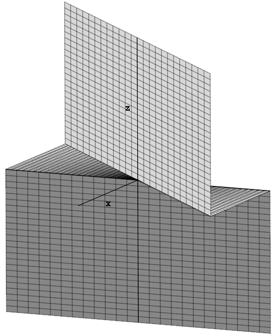
Figure 1. Image of the surface $\Gamma_{f}$ from Theorem 7.1

Remark 7.2.

We are not able to prove nor disprove that $\Gamma_{f}$ is area minimizing in a neighborhood of $(0,0,0)$.

Remark 7.3.

In a neighborhood of $(1,0)\in\mathbb{R}^{2}$, the function $f$ above is Lipschitz but not $C^{1}$. Therefore, by [8, Theorem 1.3], $f$ is not a vanishing viscosity solution of the minimal surface equation in the sense of [8, Definition 1.1]. However, $f$ is a distributional solution to the equation.

Proof of Theorem 7.1.

Point $(iv)$ is immediate. Let us prove point $(v)$. Notice that the vector field $\nu$ defined in  (17) is a calibration of $\Gamma_{f}$ in the open half-spaces $S_{1}:=\{y>\,0\}$ and $S_{2}:=\{y<\,0\}$, while $X$ is a calibration in the open half-space $S_{3}:=\{t<\,0\}$ and $\frac{X-Y}{\sqrt{2}}$ is a calibration in $S_{4}:=\{t>\,0\}$. Since every point in $\Gamma_{f}\setminus\{0\}$ belongs to one of these four open sets, $\Gamma_{f}\setminus\{0\}$ is locally area minimizing. This shows $(v)$.

Since $f$ is absolutely continuous along almost every line parallel to the coordinate axes, its distributional derivatives correspond to the pointwise derivatives:

$$\partial_{y}f(y,t)=\begin{cases}0&t\leq 0\\ -\frac{2t}{y^{2}}&0<t\leq\frac{y^{2}}{2}\\ 1&t>\frac{y^{2}}{2},\end{cases}$$

$$\partial_{t}f(y,t)=\begin{cases}0&t\leq 0\\ \frac{2}{y}&0<t\leq\frac{y^{2}}{2}\\ 0&t>\frac{y^{2}}{2},\end{cases}$$

$$\nabla^{f}f(y,t)=(\partial_{y}f+f\partial_{t}f)(y,t)=\begin{cases}0&t\leq 0\\ \frac{2t}{y^{2}}&0<t\leq\frac{y^{2}}{2}\\ 1&t>\frac{y^{2}}{2}.\end{cases}$$

It is then immediate to see that the parts $(i)$ and $(ii)$ of the theorem are true.

Part $(iii)$ follows from the Lemma 7.5 below. ∎

Lemma 7.4 (Approximation).

For $\epsilon>0$, define $f_{\epsilon}:\mathbb{R}^{2}\to\mathbb{R}$ as

$$f_{\epsilon}(y,t):=\begin{cases}0&t\leq 0\\ \frac{2yt}{y^{2}+2\epsilon}&0<t\leq\frac{y^{2}+2\epsilon}{2}\\ y&t>\frac{y^{2}+2\epsilon}{2}\end{cases}$$

Then, the following holds for every $\epsilon>0$:

1. $f_{\epsilon}\in\operatorname{Lip}_{loc}(\mathbb{R}^{2})$ and its biLipschitz Lagrangian homeomorphism $\Psi_{\epsilon}:\mathbb{R}^{2}\to\mathbb{R}^{2}$ is $\Psi(s,\tau)=(s,\chi_{\epsilon}(s,\tau))$ with $\chi_{\epsilon}(s,\tau)=\frac{a_{\epsilon}(\tau)}{2}s^{2}+\tau$, where

   $$a_{\epsilon}(\tau):=\begin{cases}0&\tau\leq 0\\ \frac{\tau}{\epsilon}&0\leq\tau\leq\epsilon\\ 1&\epsilon\leq\tau.\end{cases}$$

2. $\lim_{\epsilon\to 0^{+}}f_{\epsilon}=f$ in $W^{1,p}_{loc}(\mathbb{R}^{2})$ for all $p\in[1,3)$.

3. $\nabla^{f_{\epsilon}}f_{\epsilon}\in C^{0}(\mathbb{R}^{2})$ and $\lim_{\epsilon\to 0^{+}}\nabla^{f_{\epsilon}}f_{\epsilon}=\nabla^{f}f$ in $\mathcal{L}^{p}_{loc}(\mathbb{R}^{2})$ for all $p\in[1,\infty)$.

Proof.

Since $f_{\epsilon}$ is absolutely continuous along almost every line parallel to the coordinate axes, its distributional derivatives are

$$\partial_{y}f_{\epsilon}=\begin{cases}0&t\leq 0\\ -\frac{2t(y^{2}-2\epsilon)}{(y^{2}+2\epsilon)^{2}}&0<t\leq\frac{y^{2}+2\epsilon}{2}\\ 1&t>\frac{y^{2}+2\epsilon}{2}\end{cases}\quad\text{and}\quad\partial_{t}f_{\epsilon}=\begin{cases}0&t\leq 0\\ \frac{2y}{y^{2}+2\epsilon}&0<t\leq\frac{y^{2}+2\epsilon}{2}\\ 0&t>\frac{y^{2}+2\epsilon}{2}\end{cases}.$$

Since both $\partial_{y}f_{\epsilon}$ and $\partial_{t}f_{\epsilon}$ are bounded on bounded subsets of $\mathbb{R}^{2}$, we obtain that $f_{\epsilon}\in\operatorname{Lip}_{loc}(\mathbb{R}^{2})$. A direct computation shows that $f(s,\chi_{\epsilon}(s,\tau))=\partial_{s}\chi_{\epsilon}(s,\tau)$ for all $s,\tau\in\mathbb{R}$ and that $\Psi_{\epsilon}$ is indeed biLipschitz. So, part $(a)$ holds.

Let us now observe that $f_{\epsilon}\to f$, $\partial_{y}f_{\epsilon}\to\partial_{y}f$ and $\partial_{t}f_{\epsilon}\to\partial_{t}f$ pointwise almost everywhere in $\mathbb{R}^{2}$. Moreover, $|f_{\epsilon}|\leq g_{1}$, $|\partial_{y}f_{\epsilon}|\leq g_{2}$ and $|\partial_{t}f_{\epsilon}|\leq g_{3}$ almost everywhere in $\mathbb{R}^{2}$, where

$$g_{1}(y,t) :=|y|,\qquad g_{2}(y,t):=1,$$

$$g_{3}(y,t) :=\begin{cases}0&t\leq 0\\ \frac{2}{|y|}&0<t\leq\frac{y^{2}}{2}\\ \frac{\sqrt{2}}{\sqrt{t}}&\frac{y^{2}}{2}<t<\frac{y^{2}}{2}+1\\ 0&\frac{y^{2}}{2}+1<t.\end{cases}$$

Since, for every $L>0$ and $p\neq 2$,

$$\int_{[-L,L]^{2}}\!\!\!\!|g_{3}(y,t)|^{p}\,\mathrm{d}y\,\mathrm{d}t\!=\!\!\left(1-p\frac{2^{p-1}}{2-p}\right)\!\!\int_{-L}^{L}\!\!|y|^{2-p}\,\mathrm{d}y+\frac{2^{p}}{2-p}\!\!\int_{-L}^{L}\!\!\left(y^{2}+2\right)^{\frac{2-p}{2}}\!\!\,\mathrm{d}y,$$

then $g_{3}\in\mathcal{L}^{p}_{loc}(\mathbb{R}^{2})$ for all $1\leq p<3$. Clearly, we also have $g_{1},g_{2}\in\mathcal{L}^{p}_{loc}(\mathbb{R}^{2})$ for all $1\leq p<3$. Therefore, by the Dominated Convergence Theorem, $f_{\epsilon}\to f$ in $W^{1,p}_{loc}(\mathbb{R}^{2})$ for all $1\leq p<3$, i.e., statement $(b)$ in the lemma.

For part $(c)$, one can check by direct computation that

$$\nabla^{f_{\epsilon}}f_{\epsilon}=\begin{cases}0&t\leq 0\\ \frac{2t}{y^{2}+2\epsilon}&0<t\leq\frac{y^{2}+2\epsilon}{2}\\ 1&t>\frac{y^{2}+2\epsilon}{2}\end{cases}$$

Moreover, we have $\nabla^{f_{\epsilon}}f_{\epsilon}\to\nabla^{f}f$ in $\mathcal{L}^{p}_{loc}(\mathbb{R}^{2})$ for all $p\in[1,\infty)$. Indeed, on one hand the pointwise convergence $\nabla^{f_{\epsilon}}f_{\epsilon}$ in $\mathbb{R}^{2}$ is clear. On the other hand, $|\nabla^{f_{\epsilon}}f_{\epsilon}(y,t)|\leq 1$ for a.e. $(y,t)\in\mathbb{R}^{2}$ and for all $\epsilon\in(0,1)$, and therefore we can conclude again by the Dominated Convergence Theorem. ∎

Lemma 7.5 (Stability).

The function $f$ defined in Theorem 7.1 is stable.

Proof for “$f$ satisfies ($1^{st}$VF)”.

Let $f_{\epsilon}$ as in Lemma 7.4 and $\varphi\in C^{\infty}_{c}(\mathbb{R}^{2})$. Since $f_{\epsilon}\to f$ in $W^{1,2}_{loc}(\mathbb{R}^{2})$, then $I_{f}(\varphi)=\lim_{\epsilon\to 0}I_{f_{\epsilon}}(\varphi)$ by Lemma 2.1. By Proposition 6.1.(iii), $I_{f_{\epsilon}}(\varphi)=0$ for all $\epsilon$, thus $I_{f}(\varphi)=0$. ∎

Proof for “$f$ satisfies ($2^{nd}$VF)”.

Let $f_{\epsilon}$ and $a_{\epsilon}$ as in Lemma 7.4 and $\varphi\in C^{\infty}_{c}(\mathbb{R}^{2})$. Since $f_{\epsilon}\to f$ in $W^{1,2}_{loc}(\mathbb{R}^{2})$, then $II_{f}(\varphi)=\lim_{\epsilon\to 0}II_{f_{\epsilon}}(\varphi)$ by Lemma 2.1. By Proposition 6.1.(iv),

$$II_{f_{\epsilon}}(\varphi)=\int_{\mathbb{R}^{2}}\left[(\partial_{s}\tilde{\varphi}_{\epsilon})^{2}\frac{(\frac{a^{\prime}_{\epsilon}}{2}s^{2}+1)}{(1+a_{\epsilon}^{2})^{3/2}}-2\tilde{\varphi}_{\epsilon}^{2}\frac{a_{\epsilon}^{\prime}}{(1+a_{\epsilon}^{2})^{3/2}(\frac{a_{\epsilon}^{\prime}}{2}s^{2}+1)}\right]\,\mathrm{d}s\,\mathrm{d}\tau,$$

where we have $\tilde{\varphi}_{\epsilon}(s,\tau)=\varphi(s,\chi_{\epsilon}(s,\tau))$, $\chi_{\epsilon}(s,\tau)=\frac{a_{\epsilon}(\tau)}{2}s^{2}+\tau$ and $\tilde{f}_{\epsilon}(s,\tau)=\partial_{s}\chi_{\epsilon}(s,\tau)=a_{\epsilon}(\tau)s$. Since

$$(\partial_{s}\tilde{\varphi}_{\epsilon})^{2}\frac{(\frac{a_{\epsilon}^{\prime}}{2}s^{2}+1)}{(1+a_{\epsilon}^{2})^{3/2}}\geq 0,$$

the thesis follows if it is true that

(18) $$\limsup_{\epsilon\to 0}\int_{\mathbb{R}^{2}}\tilde{\varphi}_{\epsilon}^{2}\frac{a_{\epsilon}^{\prime}}{(1+(\partial_{s}\tilde{f}_{\epsilon})^{2})^{3/2}(\frac{a_{\epsilon}^{\prime}}{2}s^{2}+1)}\,\mathrm{d}s\,\mathrm{d}\tau\leq 0.$$

For proving (18), Recall that $a_{\epsilon}^{\prime}(\tau)=1/\epsilon$ for $\tau\in[0,\epsilon]$ and $0$ otherwise. So, if we perform the change of variables $v=\frac{s}{\sqrt{2\epsilon}}$ and $w=\frac{\tau}{\epsilon}$, we obtain

$$\int_{\mathbb{R}^{2}}\tilde{\varphi}_{\epsilon}^{2}\frac{a_{\epsilon}^{\prime}}{(1+(a_{\epsilon})^{2})^{3/2}(\frac{a_{\epsilon}^{\prime}}{2}s^{2}+1)}\,\mathrm{d}\mathcal{L}^{2}(s,\tau)\\ =\int_{\mathbb{R}}\int_{0}^{\epsilon}\varphi(s,\frac{\tau s^{2}}{2\epsilon}+\tau)^{2}\frac{1/\epsilon}{(1+(\tau/\epsilon)^{2})^{3/2}(\frac{1}{2\epsilon}s^{2}+1)}\,\mathrm{d}\tau\,\mathrm{d}s\\ =\sqrt{2\epsilon}\int_{\mathbb{R}}\int_{0}^{1}\varphi(\sqrt{2\epsilon}v,\epsilon w(v^{2}+1))^{2}\frac{1}{(1+w^{2})^{3/2}(v^{2}+1)}\,\mathrm{d}w\,\mathrm{d}v\\ \leq\sqrt{2\epsilon}M\int_{\mathbb{R}}\frac{1}{v^{2}+1}\,\mathrm{d}v\int_{0}^{1}\frac{1}{(1+w^{2})^{3/2}}\,\mathrm{d}w$$

where $M=\sup_{\mathbb{R}^{2}}\varphi^{2}$. Since $\int_{\mathbb{R}}\frac{1}{v^{2}+1}\,\mathrm{d}v\int_{0}^{1}\frac{1}{(1+w^{2})^{3/2}}\,\mathrm{d}w<\infty$, taking the limsup as $\epsilon\to 0$ we get (18). ∎

8. Second example

In this section we construct the example that proves Theorem 1.4. We summarize the results in the following statement, whose proof covers the whole section. A plot of the graph $\Gamma_{f}$ can be found in Figure 2.

Figure 2. Image of the surface $\Gamma_{f}$ from Theorem 8.1

Theorem 8.1.

Let $a:\mathbb{R}\to[0,1]$ be the function that is the Cantor staircase when restricted to $[0,1]$ and with $a(\tau)=0$ for $\tau\leq 0$, $a(\tau)=1$ for $\tau\geq 1$. Let $f\in\mathscr{C}^{1}_{\mathbb{W}}(\mathbb{R}^{2})$ be the function such that $f(s,a(\tau)s^{2}/2+\tau)=a(\tau)s$, as in Proposition 6.1. Then the following holds:

1. $f\in W^{1,2}_{loc}(\mathbb{R}^{2})\cap\mathscr{C}^{1}_{\mathbb{W}}(\mathbb{R}^{2})\cap\operatorname{Lip}_{loc}(\mathbb{R}^{2}\setminus(\{0\}\times\mathbb{R}))$.

2. $f$ is stable, but $\Gamma_{f}$ is not an intrinsic plane. The surface $\Gamma_{f}$ is locally area minimizing in $\mathbb{H}\setminus\{(0,0,z):z\in C\}$, where $C\subset[0,1]$ is the ternary Cantor set.

The fact that $\Gamma_{f}$ is not an intrinsic plane is clear. The fact that $\Gamma_{f}$ is locally area minimizing in $\mathbb{H}\setminus\{(0,0,z):z\in C\}$ is proven as in Theorem 7.1.$(v)$: More precisely, if $p\in\Gamma_{f}\setminus\{x=y=0\}$, then $\nu$ is a local calibration by Proposition 6.3; if $p\in\{(0,0,z):z\notin C\}$, then there is $U\subset\mathbb{H}$ open, $p\in U$ so that $U\cap\Gamma_{f}$ is a subset of an intrinsic plane.

The fact that $f\in\mathscr{C}^{1}_{\mathbb{W}}(\mathbb{R}^{2})\cap\operatorname{Lip}_{loc}(\mathbb{R}^{2}\setminus(\{0\}\times\mathbb{R}))$ follows from Proposition 6.1. For proving that $f$ is stable, we shall construct a Lipschitz approximation of $a$ and then complete the proof by approximation. In particular, we show through Lemma 8.2 that $f\in W^{1,2}_{loc}(\mathbb{R}^{2})$. Finally we will estimate the first and the second variations of $f$ in Lemmas 8.3 and 8.4.

Define the closed sets $C(n)\subset[0,1]$, $n\in\mathbb{N}$, inductively as follows: $C(0):=[0,1]$ and

$$C(n+1):=\frac{1}{3}C(n)\cup\left(\frac{2}{3}+\frac{1}{3}C(n)\right).$$

For $k,n\in\mathbb{N}$, define

$$C(n,k):=\begin{cases}\left[\frac{k}{3^{n}},\frac{k+1}{3^{n}}\right]&\text{if }[k/3^{n},(k+1)/3^{n}]\subset C(n)\\ \emptyset&\text{otherwise}.\end{cases}$$

Let $J_{n}$ be the collection of $k\in\{0,\dots,3^{n}\}$ such that $C(n,k)\neq\emptyset$. We have $\#J_{n}=2^{n}$ and $C(n)=\bigsqcup_{k\in J_{n}}C(n,k)$. Moreover,

$$C=\bigcap_{n=1}^{\infty}C(n)$$

is the ternary Cantor set in $[0,1]$. Set $q:=\frac{2}{3}$.

For $n\in\mathbb{N}$, let $a_{n}:\,[0,1]\to[0,1]$ be tha classical sequence of piecewise affine functions for which $a_{n}\to a$ uniformly on $[0,1]$ and $a$ agrees wiht the Cantor staircase function. A possible way for defining $(a_{n})_{n}$ is the following one. For $n\in\mathbb{N}$, define $a_{n}:\mathbb{R}\to[0,1]$ as the absolutely continuous function $a_{n}(\tau)=\int_{-\infty}^{\tau}a_{n}^{\prime}(r)\,\mathrm{d}r$, where $a_{n}^{\prime}(r):=\frac{1}{q^{n}}{\mathds{1}\!}_{C(n)}(r)$. Then $a_{n}\to a$ uniformly on $\mathbb{R}$, where $a:\mathbb{R}\to\mathbb{R}$ is the function such that $a(\tau)=0$ for $\tau\leq 0$, $a(\tau)=1$ for $\tau\geq 1$ and $a|_{[0,1]}$ is the Cantor function on the ternary Cantor set $C$. Notice that $a(\tau)=a_{n}(\tau)$ for all $\tau\in\mathbb{R}\setminus C(n)$. By continuity, the equality holds also on $\partial C(n)$.

For $y\in\mathbb{R}$ and $k\in J_{n}$ define the following subsets of $\mathbb{R}$:

$$C_{y}(n,k) :=\left\{a_{n}(\tau)\frac{y^{2}}{2}+\tau:\tau\in C(n,k)\right\}$$

$$=\left[a\left(\frac{k}{3^{n}}\right)\frac{y^{2}}{2}+\frac{k}{3^{n}},a\left(\frac{k+1}{3^{n}}\right)\frac{y^{2}}{2}+\frac{k+1}{3^{n}}\right];$$

$$C_{y}(n) :=\left\{a_{n}(\tau)\frac{y^{2}}{2}+\tau:\tau\in C(n)\right\}=\bigsqcup_{k\in J_{n}}C_{y}(n,k);$$

$$C_{y} :=\left\{a(\tau)\frac{y^{2}}{2}+\tau:\tau\in C\right\}=\bigcap_{n=1}^{\infty}C_{y}(n).$$

Notice that

$$\mathcal{L}^{1}(C_{y}(n,k) =\frac{1}{2^{n}}\left(\frac{y^{2}}{2}+q^{n}\right), \mathcal{L}^{1}(C_{y}(n)) =\frac{y^{2}}{2}+q^{n}, \mathcal{L}^{1}(C_{y}) =\frac{y^{2}}{2}.$$

For each $n\in\mathbb{N}$, define $f_{n}\in\mathscr{C}^{1}_{\mathbb{W}}$ as the function such that, for all $(s,\tau)\in\mathbb{R}^{2}$, $f_{n}\left(s,a_{n}(\tau)s^{2}/2+\tau\right)=a_{n}(\tau)s$, as in Proposition 6.1. Since $a_{n}$ is locally Lipschitz, $f_{n}$ is locally Lipschitz as well, for all $n$.

Lemma 8.2 (Approximation).

The sequence of functions $f_{n}$ defined above converge to $f$ in $W^{1,2}_{loc}(\mathbb{R}^{2})$. In particular, $f\in W^{1,2}_{loc}(\mathbb{R}^{2})$.

Proof.

First of all, we claim that $f$ is absolutely continuous along almost all coordinates lines. Indeed, by Proposition 6.1, $f$ is locally Lipschitz on $\mathbb{R}^{2}\setminus\{y=0\}$ and thus $t\mapsto f(y,t)$ is absolutely continuous if $y\neq 0$. Moreover, if $t\notin C$, then $y\mapsto f(y,t)$ is constant in a neighborhood of $0$, so it is absolutely continuous on $\mathbb{R}$. Since $\mathcal{L}^{1}(C)=0$, this completes the proof of the claim.

Therefore, the distributional derivatives $\partial_{y}f$ and $\partial_{t}f$ are functions and coincide almost everywhere with the derivatives of $f$ along the coordinates lines.

We compute

(19) $$\partial_{t}f_{n}(y,t)=\begin{cases}\frac{y}{y^{2}/2+q^{n}}&\text{if }t\in C_{y}(n)\\ 0&\text{if }t\notin C_{y}(n).\end{cases}$$

Since $a_{n}$ is piecewise affine, then $t\mapsto f_{n}(y,t)$ is also piecewise affine. If $t\notin C_{y}(n)$, then $\partial_{t}f_{n}(y,t)=0$. If $k\in J_{n}$, then $t\mapsto\partial_{t}f_{n}(y,t)$ is constant on $C_{y}(n,k)=[t_{1},t_{2}]$. Thus

$$\partial_{t}f_{n}(y,t) =\frac{f_{n}(y,t_{2})-f_{n}(y,t_{1})}{t_{2}-t_{1}}=\frac{a(\frac{k+1}{3^{n}})y-a(\frac{k}{3^{n}})y}{a(\frac{k+1}{3^{n}})y^{2}/2+\frac{k+1}{3^{n}}-a(\frac{k}{3^{n}})y^{2}/2-\frac{k}{3^{n}}}$$

$$=\frac{y}{y^{2}/2+q^{n}}$$

This shows (19). Next, we show that

(20) $$\partial_{t}f(y,t)=\begin{cases}\frac{2}{y}&\text{for a.e.\leavevmode\nobreak\ }t\in C_{y}\\ 0&\text{otherwise}.\end{cases}$$

Fix $y\in\mathbb{R}$. So, if $t\notin C_{y}$, then $t^{\prime}\mapsto f(y,t^{\prime})$ is constant in a neighborhood of $t$, hence $\partial_{t}f(y,t)=0$. If $y=0$, then $C_{0}=C$ has measure zero. Let $y\neq 0$ and $t\in C_{y}$ be such that $t^{\prime}\mapsto f(y,t^{\prime})$ is differentiable at $t$. Then, if $t=a(\tau)\frac{y^{2}}{2}+\tau$ and $t^{\prime}=a(\tau^{\prime})\frac{y^{2}}{2}+\tau^{\prime}$, we have

$$\limsup_{t^{\prime}\to t}\frac{|f(y,t^{\prime})-f(y,t)|}{|t^{\prime}-t|}=\limsup_{\tau^{\prime}\to\tau}\frac{(a(\tau^{\prime})-a(\tau))y}{(a(\tau^{\prime})-a(\tau))\frac{y^{2}}{2}+(\tau^{\prime}-\tau)}\\ \leq\frac{2}{y}\limsup_{\tau^{\prime}\to\tau}\frac{1}{1+\frac{2}{y^{2}}\frac{\tau^{\prime}-\tau}{a(\tau^{\prime})-a(\tau)}}\leq\frac{2}{y}.$$

Moreover, if $y>0$ is such that $t\mapsto f(y,t)$ is absolutely continuous, which happens for almost every $y\in\mathbb{R}$ by Proposition  6.1, from the inequalities

$$y=f(y,\frac{1}{2}y^{2}+1)=\int_{0}^{\frac{1}{2}y^{2}+1}\partial_{t}f(y,t)\,\mathrm{d}t=\int_{C_{y}}\partial_{t}f(y,t)\,\mathrm{d}t\leq\frac{2}{y}|C_{y}|=y$$

follows that $\partial_{t}f(y,t)=\frac{2}{y}$. The same strategy applies to the case $y<0$ and so we have (20).

Now we prove the first convergence, that is,

(21) $$\partial_{t}f_{n}\to\partial_{t}f\text{ in }\mathcal{L}^{2}_{loc}(\mathbb{R}^{2}).$$

We directly compute

$$\int_{0}^{\ell} \int_{\mathbb{R}}|\partial_{t}f_{n}(y,t)-\partial_{t}f(y,t)|^{2}\,\mathrm{d}t\,\mathrm{d}y$$

$$=\int_{0}^{\ell}\left[\int_{C_{y}(n)\setminus C_{y}}\left(\frac{y}{y^{2}/2+q^{n}}\right)^{2}\,\mathrm{d}t+\int_{C_{y}}\left|\frac{y}{y^{2}/2+q^{n}}-\frac{2}{y}\right|^{2}\,\mathrm{d}t\right]\,\mathrm{d}y$$

$$=\int_{0}^{\ell}\left[\left(\frac{y}{y^{2}/2+q^{n}}\right)^{2}\left(|C_{y}(n)|-|C_{y}|\right)+\left|\frac{y}{y^{2}/2+q^{n}}-\frac{2}{y}\right|^{2}|C_{y}|\right]\,\mathrm{d}y$$

$$=q^{n}\int_{0}^{\ell}\left(\frac{y}{y^{2}/2+q^{n}}\right)^{2}\,\mathrm{d}y+2q^{2n}\int_{0}^{\ell}\frac{1}{(y^{2}/2+q^{n})^{2}}\,\mathrm{d}y$$

$$=4q^{n}\int_{0}^{\ell}\frac{1}{y^{2}/2+q^{n}}\,\mathrm{d}y$$

$$=2\int_{0}^{\ell/\sqrt{2q^{n}}}\frac{\sqrt{2q^{n}}}{x^{2}+1}\,\mathrm{d}x=2\sqrt{2}q^{n/2}\arctan\left(\frac{\ell}{\sqrt{2}}q^{-n/2}\right),$$

The last expression goes to $0$ as $n\to\infty$, and so (21) is proven.

The next step is to show that

(22) $$f_{n}\to f\text{ and }\nabla^{f_{n}}f_{n}\to\nabla^{f}f\text{ uniformly on compact sets}.$$

First of all, if $\epsilon>0$ and $K>0$, then there is $N>0$ such that for all $t\in\mathbb{R}$, all $y\in\mathbb{R}$ with $|y|\leq K$ and all $n\geq N$ there are $\tau_{1},\tau_{2}\in\mathbb{R}\setminus C(n)$ such that

$$t_{1}:=a(\tau_{1})\frac{y^{2}}{2}+\tau_{1}\leq t\leq a(\tau_{2})\frac{y^{2}}{2}+\tau_{2}=:t_{2},$$

and $a(\tau_{2})-a(\tau_{1})\leq\epsilon$.

Secondly, notice that $a_{n}=a$ on $\mathbb{R}\setminus C(n)$. So,

$$\nabla^{f_{n}}f_{n}(y,t)-\nabla^{f}f(y,t)\leq\nabla^{f_{n}}f_{n}(y,t_{2})-\nabla^{f}f(y,t_{1})=a(\tau_{2})-a(\tau_{1})\leq\epsilon,$$

$$\nabla^{f}f(y,t)-\nabla^{f_{n}}f_{n}(y,t)\leq\nabla^{f}f(y,t_{2})-\nabla^{f_{n}}f_{n}(y,t_{1})=a(\tau_{2})-a(\tau_{1})\leq\epsilon.$$

Therefore, there is $N\in\mathbb{N}$ such that for all $(y,t)\in\mathbb{R}^{2}$ with $|y|\leq K$ and all $n\geq N$, $|\nabla^{f_{n}}f_{n}(y,t)-\nabla^{f}f(y,t)|\leq\epsilon$, i.e., $\nabla^{f_{n}}f_{n}\to\nabla^{f}f$ uniformly on compact sets.

Next, notice that $f(y,t)=\nabla^{f}f(y,t)\,y$ and $f_{n}(y,t)=\nabla^{f_{n}}f_{n}(y,t)\,y$. Therefore, $f_{n}\to f$ uniformly on compact sets as well and (22) is proven.

Finally, we conclude that

(23) $$\partial_{y}f_{n}\to\partial_{y}f\text{ in }\mathcal{L}^{2}_{loc}(\mathbb{R}^{2}).$$

Indeed, since $f$ is ACL, we have, whenever $\nabla f_{n}$ exist for all $n$,

$$\partial_{y}f_{n}=\nabla^{f_{n}}f_{n}-f_{n}\partial_{t}f_{n}.$$

Since the right hand side converges to $\partial_{y}f$ in $\mathcal{L}^{2}_{loc}(\mathbb{R}^{2})$, the left hand side does the same. The proof is complete. ∎

Lemma 8.3.

The function $f$ satisfies ($1^{st}$VF).

Proof.

Let $f_{n}$ as above and $\varphi\in C^{\infty}_{c}(\mathbb{R}^{2})$. Since $f_{n}\to f$ in $W^{1,2}_{loc}(\mathbb{R}^{2})$, then $I_{f}(\varphi)=\lim_{n\to\infty}I_{f_{n}}(\varphi)$ by Lemma 2.1. By Proposition 6.1.(iii), $I_{f_{n}}(\varphi)=0$ for all $n$, thus $I_{f}(\varphi)=0$. ∎

Lemma 8.4.

The function $f$ satisfies ($2^{nd}$VF).

Proof.

Fix $\varphi\in\mathscr{C}^{\infty}_{c}(\mathbb{R}^{2})$. Since $f_{n}\to f$ in $W^{1,2}_{loc}(\mathbb{R}^{2})$ and $\nabla^{f_{n}}f_{n}\to\nabla^{f}f$ uniformly on compact sets, then

$$II_{f}(\varphi)=\lim_{n\to\infty}II_{f_{n}}(\varphi).$$

Since $a_{n}$ is locally Lipschitz, by Proposition 6.1.$(iv)$, we have

$$II_{f_{n}}(\varphi)=\int_{\mathbb{R}^{2}}(\partial_{s}\tilde{\varphi}_{n})^{2}\frac{(\frac{a_{n}^{\prime}}{2}s^{2}+1)}{(1+a_{n}^{2})^{3/2}}-2\tilde{\varphi}_{n}^{2}\frac{a_{n}^{\prime}}{(1+(a_{n})^{2})^{3/2}(\frac{a_{n}^{\prime}}{2}s^{2}+1)}\,\mathrm{d}s\,\mathrm{d}\tau,$$

where $\tilde{\varphi}_{n}(s,\tau):=\varphi(s,a_{n}(\tau)\frac{s^{2}}{2}+\tau)$. So, we only need to show that

$$\limsup_{n\to\infty}\int_{\mathbb{R}^{2}}\tilde{\varphi}_{n}^{2}\frac{a_{n}^{\prime}}{(1+(a_{n})^{2})^{3/2}(\frac{a_{n}^{\prime}}{2}t^{2}+1)}\,\mathrm{d}t\,\mathrm{d}\tau\leq 0.$$

Let $M:=\sup_{p\in\mathbb{R}^{2}}\varphi(p)^{2}$. Then

$$\int_{\mathbb{R}^{2}}\tilde{\varphi}_{n}^{2}\frac{a_{n}^{\prime}}{(1+(a_{n})^{2})^{3/2}(\frac{a_{n}^{\prime}}{2}s^{2}+1)}\,\mathrm{d}t\,\mathrm{d}\tau\\ \leq M\int_{C(n)}\frac{a_{n}^{\prime}}{(1+(a_{n})^{2})^{3/2}}\int_{\mathbb{R}}\frac{1}{(\frac{a_{n}^{\prime}}{2}s^{2}+1)}\,\mathrm{d}t\,\mathrm{d}\tau$$

If $\tau\in C(n)$, then $a_{n}^{\prime}=q^{-n}$ and, after substituting $v=\sqrt{\frac{1}{2q^{n}}}s$, $\,\mathrm{d}v=\sqrt{\frac{1}{2q^{n}}}\,\mathrm{d}s$

$$\int_{\mathbb{R}}\frac{1}{(\frac{a_{n}^{\prime}}{2}s^{2}+1)}\,\mathrm{d}s=\int_{\mathbb{R}}\frac{\sqrt{2q^{n}}}{v^{2}+1}\,\mathrm{d}v=\sqrt{2q^{n}}\pi.$$

Moreover,

$$\int_{C(n)}\frac{a_{n}^{\prime}}{(1+(a_{n})^{2})^{3/2}}\,\mathrm{d}\tau=\sum_{k\in J_{k}}\int_{\frac{k}{3^{n}}}^{\frac{k+1}{3^{n}}}\frac{a_{n}^{\prime}}{(1+(a_{n})^{2})^{3/2}}\,\mathrm{d}\tau$$

For each $k\in J_{k}$, make the substitution $v=a_{n}(\tau)$, $\,\mathrm{d}v=a_{n}^{\prime}\,\mathrm{d}\tau$, $\frac{k}{3^{n}}\mapsto a_{n}(\frac{k}{3^{n}})=a(\frac{k}{3^{n}})$, $\frac{k+1}{3^{n}}\mapsto a_{n}(\frac{k+1}{3^{n}})=a(\frac{k+1}{3^{n}})$

$$\int_{\frac{k}{3^{n}}}^{\frac{k+1}{3^{n}}}\frac{a_{n}^{\prime}}{(1+(a_{n})^{2})^{3/2}}\,\mathrm{d}\tau=\int_{a(\frac{k}{3^{n}})}^{a(\frac{k+1}{3^{n}})}\frac{1}{(1+v^{2})^{3/2}}\,\mathrm{d}v$$

So,

$$\sum_{k\in J_{k}}\int_{\frac{k}{3^{n}}}^{\frac{k+1}{3^{n}}}\frac{a_{n}^{\prime}}{(1+(a_{n})^{2})^{3/2}}\,\mathrm{d}\tau=\int_{0}^{1}\frac{1}{(1+v^{2})^{3/2}}\,\mathrm{d}v=\frac{1}{\sqrt{2}}.$$

All in all, we have

$$\limsup_{n\to\infty}\int_{\mathbb{R}^{2}}\varphi_{n}^{2}\frac{a_{n}^{\prime}}{(1+(a_{n})^{2})^{3/2}(\frac{a_{n}^{\prime}}{2}s^{2}+1)}\,\mathrm{d}s\,\mathrm{d}\tau\leq\limsup_{n\to\infty}M\sqrt{q^{n}}\pi=0.$$

∎

References

- [1] G. Alberti, S. Bianchini and L. Caravenna “Eulerian, Lagrangian and Broad continuous solutions to a balance law with non-convex flux I” In J. Differential Equations 261.8, 2016, pp. 4298–4337 DOI: 10.1016/j.jde.2016.06.026
- [2] Luigi Ambrosio “Some fine properties of sets of finite perimeter in Ahlfors regular metric measure spaces” In Adv. Math. 159.1, 2001, pp. 51–67 DOI: 10.1006/aima.2000.1963
- [3] Luigi Ambrosio and Roberta Ghezzi “Sobolev and bounded variation functions on metric measure spaces” In Geometry, analysis and dynamics on sub-Riemannian manifolds. Vol. II, EMS Ser. Lect. Math. Eur. Math. Soc., Zürich, 2016, pp. 211–273
- [4] Luigi Ambrosio, Francesco Serra Cassano and Davide Vittone “Intrinsic regular hypersurfaces in Heisenberg groups” In J. Geom. Anal. 16.2, 2006, pp. 187–232 DOI: 10.1007/BF02922114
- [5] Luigi Ambrosio and Paolo Tilli “Topics on analysis in metric spaces” 25, Oxford Lecture Series in Mathematics and its Applications Oxford University Press, Oxford, 2004, pp. viii+133
- [6] Vittorio Barone Adesi, Francesco Serra Cassano and Davide Vittone “The Bernstein problem for intrinsic graphs in Heisenberg groups and calibrations” In Calc. Var. Partial Differential Equations 30.1, 2007, pp. 17–49 DOI: 10.1007/s00526-006-0076-3
- [7] F. Bigolin, L. Caravenna and F. Serra Cassano “Intrinsic Lipschitz graphs in Heisenberg groups and continuous solutions of a balance equation” In Ann. Inst. H. Poincaré Anal. Non Linéaire 32.5, 2015, pp. 925–963 DOI: 10.1016/j.anihpc.2014.05.001
- [8] Luca Capogna, Giovanna Citti and Maria Manfredini “Regularity of non-characteristic minimal graphs in the Heisenberg group ” In Indiana Univ. Math. J. 58.5, 2009, pp. 2115–2160 DOI: 10.1512/iumj.2009.58.3673
- [9] Luca Capogna, Giovanna Citti and Maria Manfredini “Smoothness of Lipschitz minimal intrinsic graphs in Heisenberg groups , ” In J. Reine Angew. Math. 648, 2010, pp. 75–110 DOI: 10.1515/CRELLE.2010.080
- [10] Luca Capogna, Donatella Danielli and Nicola Garofalo “The geometric Sobolev embedding for vector fields and the isoperimetric inequality” In Comm. Anal. Geom. 2.2, 1994, pp. 203–215 DOI: 10.4310/CAG.1994.v2.n2.a2
- [11] Luca Capogna, Donatella Danielli, Scott D. Pauls and Jeremy T. Tyson “An introduction to the Heisenberg group and the sub-Riemannian isoperimetric problem” 259, Progress in Mathematics Birkhäuser Verlag, Basel, 2007, pp. xvi+223
- [12] Jih-Hsin Cheng, Jenn-Fang Hwang and Paul Yang “Existence and uniqueness for -area minimizers in the Heisenberg group” In Math. Ann. 337.2, 2007, pp. 253–293 DOI: 10.1007/s00208-006-0033-7
- [13] Jih-Hsin Cheng, Jenn-Fang Hwang and Paul Yang “Regularity of smooth surfaces with prescribed -mean curvature in the Heisenberg group” In Math. Ann. 344.1, 2009, pp. 1–35 DOI: 10.1007/s00208-008-0294-4
- [14] Jih-Hsin Cheng, Jenn-Fang Hwang, Andrea Malchiodi and Paul Yang “Minimal surfaces in pseudohermitian geometry” In Ann. Sc. Norm. Super. Pisa Cl. Sci. (5) 4.1, 2005, pp. 129–177
- [15] D. Danielli, N. Garofalo, D. M. Nhieu and S. D. Pauls “Instability of graphical strips and a positive answer to the Bernstein problem in the Heisenberg group ” In J. Differential Geom. 81.2, 2009, pp. 251–295 URL: http://projecteuclid.org/euclid.jdg/1231856262
- [16] Donatella Danielli, Nicola Garofalo, Duy-Minh Nhieu and Scott D. Pauls “The Bernstein problem for embedded surfaces in the Heisenberg group ” In Indiana Univ. Math. J. 59.2, 2010, pp. 563–594 DOI: 10.1512/iumj.2010.59.4291
- [17] Lawrence C. Evans and Ronald F. Gariepy “Measure theory and fine properties of functions”, Textbooks in Mathematics CRC Press, Boca Raton, FL, 2015, pp. xiv+299
- [18] Mattia Fogagnolo, Roberto Monti and Davide Vittone “Variation formulas for -rectifiable sets” In Ann. Acad. Sci. Fenn. Math. 42.1, 2017, pp. 239–256 DOI: 10.5186/aasfm.2017.4220
- [19] Bruno Franchi, Raul Serapioni and Francesco Serra Cassano “Rectifiability and perimeter in the Heisenberg group” In Math. Ann. 321.3, 2001, pp. 479–531 DOI: 10.1007/s002080100228
- [20] Matteo Galli and Manuel Ritoré “Area-stationary and stable surfaces of class in the sub-Riemannian Heisenberg group ” In Adv. Math. 285, 2015, pp. 737–765 DOI: 10.1016/j.aim.2015.08.008
- [21] R.F. Gariepy and W.P. Ziemer “Modern Real Analysis” PWS Pub., 1995 URL: https://books.google.co.uk/books?id=CBQNNQAACAAJ
- [22] N. Garofalo and S. D. Pauls “The Bernstein Problem in the Heisenberg Group” In ArXiv Mathematics e-prints, 2002 eprint: math/0209065
- [23] Nicola Garofalo and Duy-Minh Nhieu “Isoperimetric and Sobolev inequalities for Carnot-Carathéodory spaces and the existence of minimal surfaces” In Comm. Pure Appl. Math. 49.10, 1996, pp. 1081–1144 DOI: 10.1002/(SICI)1097-0312(199610)49:10<1081::AID-CPA3>3.0.CO;2-A
- [24] Sebastiano Golo “Some remarks on contact variations in the first Heisenberg group” In Ann. Acad. Sci. Fenn. Math. 43.1, 2018, pp. 311–335
- [25] Philip Hartman “Ordinary differential equations” 38, Classics in Applied Mathematics Society for IndustrialApplied Mathematics (SIAM), Philadelphia, PA, 2002, pp. xx+612 DOI: 10.1137/1.9780898719222
- [26] Stanislav Hencl and Pekka Koskela “Lectures on mappings of finite distortion” 2096, Lecture Notes in Mathematics Springer, Cham, 2014 DOI: 10.1007/978-3-319-03173-6
- [27] Ana Hurtado, Manuel Ritoré and César Rosales “The classification of complete stable area-stationary surfaces in the Heisenberg group ” In Adv. Math. 224.2, 2010, pp. 561–600 DOI: 10.1016/j.aim.2009.12.002
- [28] Bernd Kirchheim and Francesco Serra Cassano “Rectifiability and parameterization of intrinsic regular surfaces in the Heisenberg group” In Ann. Sc. Norm. Super. Pisa Cl. Sci. (5) 3.4, 2004, pp. 871–896
- [29] Roberto Monti “Isoperimetric problem and minimal surfaces in the Heisenberg group” In Geometric measure theory and real analysis 17, CRM Series Ed. Norm., Pisa, 2014, pp. 57–129
- [30] Roberto Monti “Minimal surfaces and harmonic functions in the Heisenberg group” In Nonlinear Anal. 126, 2015, pp. 378–393 DOI: 10.1016/j.na.2015.03.013
- [31] Roberto Monti, Francesco Serra Cassano and Davide Vittone “A negative answer to the Bernstein problem for intrinsic graphs in the Heisenberg group” In Boll. Unione Mat. Ital. (9) 1.3, 2008, pp. 709–727
- [32] Roberto Monti and Giorgio Stefani “Improved Lipschitz approximation of -perimeter minimizing boundaries” In J. Math. Pures Appl. (9) 108.3, 2017, pp. 372–398 DOI: 10.1016/j.matpur.2017.04.002
- [33] Roberto Monti and Davide Vittone “Height estimate and slicing formulas in the Heisenberg group” In Anal. PDE 8.6, 2015, pp. 1421–1454 DOI: 10.2140/apde.2015.8.1421
- [34] Pierre Pansu “Géométrie du groupe de Heisenberg”, 1982
- [35] Pierre Pansu “Métriques de Carnot-Carathéodory et quasiisométries des espaces symétriques de rang un” In Ann. of Math. (2) 129.1, 1989, pp. 1–60 DOI: 10.2307/1971484
- [36] Pierre Pansu “Une inégalité isopérimétrique sur le groupe de Heisenberg” In C. R. Acad. Sci. Paris Sér. I Math. 295.2, 1982, pp. 127–130
- [37] Scott D. Pauls “-minimal graphs of low regularity in ” In Comment. Math. Helv. 81.2, 2006, pp. 337–381 DOI: 10.4171/CMH/55
- [38] Scott D. Pauls “Minimal surfaces in the Heisenberg group” In Geom. Dedicata 104, 2004, pp. 201–231 DOI: 10.1023/B:GEOM.0000022861.52942.98
- [39] M. Ritoré and C. Rosales “Area-stationary and stable surfaces in the sub-Riemannian Heisenberg group ” In Mat. Contemp. 35, 2008, pp. 185–203
- [40] Manuel Ritoré “Examples of area-minimizing surfaces in the sub-Riemannian Heisenberg group with low regularity” In Calc. Var. Partial Differential Equations 34.2, 2009, pp. 179–192 DOI: 10.1007/s00526-008-0181-6
- [41] Francesco Serra Cassano “Some topics of geometric measure theory in Carnot groups” In Geometry, analysis and dynamics on sub-Riemannian manifolds. Vol. 1, EMS Ser. Lect. Math. Eur. Math. Soc., Zürich, 2016, pp. 1–121
- [42] Francesco Serra Cassano and Davide Vittone “Graphs of bounded variation, existence and local boundedness of non-parametric minimal surfaces in Heisenberg groups” In Adv. Calc. Var. 7.4, 2014, pp. 409–492 DOI: 10.1515/acv-2013-0105
- [43] William P. Ziemer “Modern real analysis” With contributions by Monica Torres 278, Graduate Texts in Mathematics Springer, Cham, 2017, pp. xi+382