Cosmological constraints on $\Lambda(\alpha)$CDM models with time-varying fine structure constant

Abstract

We study the $\Lambda(\alpha)$CDM models with $\Lambda(\alpha)$ being a function of the time-varying fine structure constant $\alpha$. We give a close look at the constraints on two specific $\Lambda(\alpha)$CDM models with one and two model parameters, respectively, based on the cosmological observational measurements along with 313 data points for the time-varying $\alpha$. We find that the model parameters are constrained to be around $10^{-4}$, which are similar to the results discussed previously but more accurately.

I Introduction

The cosmological constant ($\Lambda$) was first introduced to the general theory of relativity by Einstein 1EINSTEN more than one hundred years ago 100yrs . Nowadays, it is contained in the standard model of cosmology: $\Lambda$ cold dark matter ($\Lambda$CDM), which is the simplest way to act as dark energy DE to explain the current accelerated expanding universe discovered in 1998 Riess:1998cb ; Perlmutter:1998np . However, in the $\Lambda$CDM model there is a well known cosmological constant problem, related to the two theoretical difficulties of “coincidence” Ostriker:1995rn ; ArkaniHamed:2000tc and “fine-tuning” Weinberg:1988cp ; WBook . Note that the fine-tuning one is about the question of “why the non-zero cosmological constant is so tiny,” which was known even before the proposal of dark energy in 1998 Weinberg:1988cp ; WBook . Although it is believed that the $\Lambda$ problem can be ultimately solved only in a unified theory of quantum gravity and the standard model of electroweak and strong interactions in particle physics, there have been many attempts trying to understand this problem in resent years 100yrs ; Weinberg:1988cp ; Review1 . In particular, the axiomatic approach 9:Beck:2008rd is one of the most interesting ideas, in which $\Lambda$ is derived from four axioms 11 ; Boehmer:2005sm ; Wesson:2003qn ; Boehmer:2006fd , in close analogy to the Khinchin axioms at the information theory 15 ; 16 ; 17 ; 18 .

From the four natural and simple axioms, the explicit form of the cosmological constant is given by 9:Beck:2008rd

$$\Lambda=\frac{G^{2}}{\hbar^{4}}\left(\frac{m_{e}}{\alpha}\right)^{6}.$$ (1)

where $G$ is the gravitational constant, $\hbar$ is the reduced Planck constant, $m_{e}$ is the electron mass, and $\alpha$ is the fine structure constant. Note that the relation in Eq. (1) has also been independently given in Ref. Boehmer:2005sm . In 1998, along with the discovery of the accelerated expansion universe, an evidence of the time variation of $\alpha$ was found Webb:1998cq ; Webb:2000mn , namely ${\Delta\alpha}/{\alpha}\equiv({\alpha-\alpha_{0}})/{\alpha_{0}}$ is non-zero with $\alpha_{0}$ being the present value of $\alpha$. It was claimed that $\alpha$ is not only a time varying parameter but a spatially varying one King:2012id ; Webb:2010hc . As a result, in terms of Eq. (1) with $\Lambda\propto\alpha^{-6}$, the cosmological constant term should be time and space-dependent too Uzan:2010pm ; Webb:1998cq ; Wei:2009xg ; Wei:2011jw ; Terazawa:2012fa ; 60 . In this case, it might be responsible for the possible anisotropy in the accelerated expansion of the universe.

Recently, a time-varying fine structure constant $\alpha$ has been extensively discussed in the literature Uzan:2010pm ; Wei:2009xg ; Wei:2011jw ; 60 ; Terazawa:2012fa . In this scenario, $\alpha$ is only time-dependent and increasing with time Webb:1998cq ; Webb:2000mn ; Murphy:2000pz . In this paper, unlike the general $\Lambda(t)$ models without explicit forms, we take those models with $\Lambda(\alpha)\propto\alpha^{-6}$ in Eq. (1) to study the time-varying effects.

In our numerical calculations, we use the CAMB Lewis:1999bs and CosmoMC Lewis:2002ah packages with the Markov chain Monte Carlo (MCMC) method to give a close look at the models by including 313 data points of ${\Delta\alpha}/{\alpha}$ King:2012id ; 30 ; 31 ; 32 ; Wilczynska:2015una in CosmoMC. Comparing with the previous study in Ref. Wei:2016moy , our analysis starts with a different method of the projection and a variety of the observational datasets together with adding 20 new data points Wilczynska:2015una for ${\Delta\alpha}/{\alpha}$, resulting in a more accurate outcome.

This paper is organized as follows. In Sec. II, we introduce the varying cosmological constant $\Lambda(\alpha)\propto\alpha^{-6}$ and derive the evolution equations for pressureless matter in the linear perturbation theory. In Sec. III, we perform the numerical calculations to obtain the observational constraints on the model parameters as well as cosmological observables based on the datasets. Our conclusions are given in Sec. IV.

II Varying cosmological constant models

II.1 Formalism

We consider a spatially flat Friedmann-Robertson-Walker (FRW) universe with the metric Cai:2010hk

$$ds^{2}=-dt^{2}+a^{2}(t)(dr^{2}+r^{2}d{\Omega})\$$ (2)

containing only dark or vacuum energy and pressureless matter with the Friedmann equations, given by

$$H^{2}=\frac{8\pi G}{3}(\rho_{m}+\rho_{\Lambda})\,,$$ (3)

$$\dot{H}=-4\pi G(\rho_{m}+\rho_{\Lambda}+P_{m}+P_{\Lambda}),\,$$ (4)

where $H=da/(adt)$ is the Hubble parameter with $a$ the scale factor, $\rho_{m}$ is the energy density of pressureless matter, $\rho_{\Lambda}=c^{4}\Lambda/(8\pi G)$ is the energy density of dark energy, and $P_{m(\Lambda)}$ is the pressure of pressureless matter (dark energy). We will describe the varying cosmological constant scenarios in terms of $\rho_{\Lambda}$ instead of $\Lambda$. In the models, the equation-of-state (EoS) of dark energy (pressureless matter) is given by $w_{\Lambda(m)}={P_{\Lambda(m)}}/{\rho_{\Lambda(m)}}=-1(0)$.

In this study, we assume that only the fine structure “constant” $\alpha=e^{2}/(\hbar c)$ is varying in time due to the change of the electric charge $e$, whereas the other fundamental constants $\hbar,G,c$ and $m_{e}$ are true constants. Consequently, $\rho_{\Lambda},\Lambda(\alpha)$ and $\alpha$ are related by $\rho_{\Lambda}\propto\Lambda(\alpha)\propto\alpha^{-6}$, which leads to

$$\frac{\dot{\rho}_{\Lambda}}{\rho_{\Lambda}}=-6\,\frac{\dot{\alpha}}{\alpha}\,.$$ (5)

The vacuum energy interacts with pressureless matter by exchanging energy between them with the continuity equations, written as

$$\dot{\rho}_{m}+3H\rho_{m}=Q\,,$$ (6)

$$\dot{\rho}_{\Lambda}=-Q\,,$$ (7)

where the coupling term $Q=6{\rho}_{\Lambda}\dot{\alpha}/\alpha\neq 0$ from Eq. (5). The total energy conservation equation is given by $\dot{\rho}_{tot}+3H(\rho_{tot}+P_{tot})=0$, where ${\rho}_{tot}=\rho_{m}+\rho_{\Lambda}$ and $P_{tot}=P_{\Lambda}$.

Inspired by the discussions in Refs. Dalal:2001dt ; Guo:2007zk ; Wei:2010uh , the character of the $\Lambda(\alpha)$CDM models is given by

$$\frac{\rho_{\Lambda}}{\rho_{m}}=f(a),$$ (8)

where $f(a)$ can be any function of the scale factor $a$. For $f(a)\propto a^{3}$, the coupling parameter $Q$ in Eqs. (6) and (7) vanishes so that ${\rho_{\Lambda}}$ is a constant and $\rho_{m}\propto a^{-3}$, representing the $\Lambda$CDM model. From Eqs. (3) and (8), we obtain

$$\Omega_{\Lambda}\equiv{8\pi G\rho_{\Lambda}\over 3H^{2}}=\frac{f}{1+f},$$ (9)

$$\Omega_{m}\equiv{8\pi G\rho_{m}\over 3H^{2}}=\frac{1}{1+f}\,,$$ (10)

so that $\Omega_{m}+\Omega_{\Lambda}=1$. Substituting Eq. $\eqref{eq:fa}$ into Eq. $\eqref{eq:eos1}$ along with Eqs. (9) and (10), we get

$$Q=-H\rho_{m}\Omega_{\Lambda}\left(a\frac{f^{\prime}}{f}-3\right)=-H\rho_{\Lambda}\Omega_{m}\left(a\frac{f^{\prime}}{f}-3\right),$$ (11)

where the prime “$\prime$” stands for a derivative with respect to $a$. Subsequently, from Eqs. $\eqref{eq:friedmann1}$ and $\eqref{eq:12}$ we derive that

$$\frac{\Delta\alpha}{\alpha}\equiv\frac{\alpha-\alpha_{0}}{\alpha_{0}}=\left(\frac{\Omega_{\Lambda}H^{2}}{H_{0}^{2}(1-\Omega_{m0})}\right)^{-1/6}-1,$$ (12)

where the quantities with the subscript “0” correspond to those with $a=1$. It is clear that, in the case of the $\Lambda$CDM model with $f\propto\alpha^{3}$, ${\Delta\alpha}/{\alpha}=0$, implying a constant ${\alpha}$.

We now explore the possible forms for the $\Lambda(\alpha)$CDM models with a time-varying ${\alpha}$. First of all, $f(a)$ at present time with $a=1$ is given by

$$f_{0}=f(a=1)=\frac{\rho_{\Lambda 0}}{\rho_{m0}}=\frac{1}{\Omega_{m0}}-1.$$ (13)

To simplify our discussions without loss of generality, we consider

$$f(a)=f_{0}a^{\xi(a)},$$ (14)

where $\xi(a)$ is a function of $a$. For $\xi(a)=3$, it reduces to the $\Lambda$CDM model with the constant $\alpha$. Obviously, it is expected that $\xi(a)$ should be close to 3 so that the model does not deviate from the $\Lambda$CDM too much as required by the cosmological data. From Eqs. (9) and (10), we obtain the explicit form

$$\frac{H^{2}}{H_{0}^{2}}=a^{-3}\left[\Omega_{m0}+(1-\Omega_{m0})a^{\xi(a)}\right]^{3/{\xi(a)}}.$$ (15)

Consequently, we can derive that

$$\rho_{\Lambda} = \rho_{\Lambda 0}\frac{f}{(1+f)(1-\Omega_{m0})}\frac{H^{2}}{H_{0}^{2}}=\rho_{\Lambda 0}a^{\xi(a)-3}\left[(1-\Omega_{m0})a^{\xi(a)}+\Omega_{m0}\right]^{3/{\xi(a)}-1}\,,$$ (16)

$$\rho_{m} = \frac{\rho_{\Lambda}}{f(a)}=\rho_{m0}a^{-3}\left[(1-\Omega_{m0})a^{\xi(a)}+\Omega_{m0}\right]^{3/{\xi(a)}-1}\,.$$ (17)

Similar to the Chevallier-Polarski-Linder (CPL) EoS parameterization of $w=w_{0}+w_{a}(1-a)$ CPL , we take the simplest form for $\xi(a)$ to be CPL-like, given by

$$\xi(a)=\xi_{0}+\xi_{1}(1-a),$$ (18)

with $\xi_{0}=3+u_{0}$. As $\xi(a)$ is close to 3, $u_{0}\to 0$. The function for $\xi(a)$ in Eq. (18) is labelled as $\Lambda(\alpha)$CDM1. Note that this $\Lambda(\alpha)$CDM model along with the special case with $\xi_{1}=0$ has been discussed in Ref. Wei:2016moy . The relation of $\xi_{1}$ and ${\Delta\alpha}/{\alpha}$ can be explicitly written as

$$\xi_{1}=\frac{\ln\left(a^{\xi_{0}}(f_{0}+1)({\Delta\alpha\over\alpha}+1)^{6}\frac{H^{2}}{H_{0}^{2}}-f_{0}a^{\xi_{0}}\right)}{(a-1)\ln a}\,,$$ (19)

It is easy to check that if $\Delta\alpha/\alpha$=0, the model becomes $\Lambda$CDM with $\xi_{0}=3$ and $\xi_{1}=0$.

To illustrate the feature of $\xi(a)$, we also consider $u_{0}=0$ in Eq. (18), and refer to the resulting function of

$${\xi(a)}=3+\xi_{1}(1-a),$$ (20)

as $\Lambda(\alpha)$CDM2, which was not studied in Ref. Wei:2016moy . In the following, we will concentrate on the two models of $\Lambda(\alpha)$CDM1 and $\Lambda(\alpha)$CDM2.

II.2 Linear perturbation theory

In order to consider whether the models can be established in the dynamical universe, the linear perturbation theory should be taken into account to examine the dynamics of the $\Lambda(\alpha)$CDM models. Here, we will study the growth equations of the density perturbation for the models based on the standard linear perturbation theory Ma:1995ey . In the synchronous gauge, the metric is given by

$$ds^{2}=a^{2}(\tau)[-d\tau^{2}+(\delta_{ij}+h_{ij})dx^{i}dx^{j}],$$ (21)

where $i,j=1,2,3$, $\tau$ is the conformal time, and

$$h_{ij}=\int d^{3}ke^{i\vec{k}\vec{x}}\left[\hat{k}_{i}\hat{k}_{j}h(\vec{k},\tau)+6\left(\hat{k}_{i}\hat{k}_{j}-\frac{1}{3}\delta_{ij}\right)\eta(\vec{k},\tau)\right]\,,$$ (22)

with the $k$-space unit vector of $\hat{k}=\vec{k}/k$ and two scalar perturbations of $h(\vec{k},\tau)$ and $\eta(\vec{k},\tau)$. From the conservation equation of $\nabla^{\nu}(T^{m}_{\mu\nu}+T^{\Lambda}_{\mu\nu})=0$ with $\delta T^{0}_{0}=\delta\rho_{m}$, $\delta T^{0}_{i}=-T^{i}_{0}=(\rho_{m}+P_{m})v^{i}_{m}$ and $\delta T^{i}_{j}=\delta P_{m}\delta^{i}_{j}$.

As explicitly shown in Refs. DEP2 ; Grande:2008re , there are two basic perturbation equations, given by

$$\sum_{i=\Lambda,m}\delta\rho_{i}+3\delta(\frac{H}{a})(\rho_{i}+P_{i})+3\frac{H}{a}(\delta\rho_{i}+\delta P_{i})=0,$$ (23)

$$\sum_{i=\Lambda,m}\dot{\theta}_{i}(\rho_{i}+P_{i})+\theta_{i}(\dot{\rho}_{i}+\dot{P}_{i}+5H(\rho_{i}+P_{i}))=\frac{k^{2}}{a}\sum_{i=\Lambda,m}\delta P_{i},$$ (24)

where $H=da/(ad\tau)$ in terms of conformal time $\tau$, $\delta\rho_{i}$ represent the density fluctuations, and $\theta_{i}$ are the corresponding velocities. As there is no peculiar velocity for dark energy, we take $\theta_{\Lambda}=0$. In addition, we assume that $\delta\rho_{m}\gg\delta\rho_{\Lambda}$ and $\delta\dot{\rho}_{m}\gg\delta\dot{\rho}_{\Lambda}$ in our models. From Eqs. (24), we get

$${\dot{\theta}_{m}}+{\theta}_{m}({2H}-\frac{\dot{\rho}_{\Lambda}}{{\rho}_{m}})=-\frac{k^{2}}{a}\frac{\delta\rho_{\Lambda}}{\rho_{m}},$$ (25)

resulting in the momentum conservation equation in this gauge, given by

$$\dot{v}_{m}+Hv_{m}+v_{m}\frac{\dot{\rho}_{\Lambda}}{{\rho}_{m}}=\frac{\delta\rho_{\Lambda}}{\rho_{m}},$$ (26)

based on $\theta_{m}=-{k^{2}}v_{m}/{a}+{\cal O}(2)$ with ${\cal O}(2)$ referring to the second order perturbations. Due to the remaining gauge freedom left Wang:2014xca ; Wang:2013qy in the synchronous gauge, one can take the zero velocity of matter, $i.e.$, $v_{m}=0$, which leads to $\delta\rho_{\Lambda}=\theta_{m}=0$. As a result, in our calculations we can choose that $\delta\rho_{\Lambda}\to 0$ and $\theta_{m}\to 0$. For the matter perturbation, the growth equations are given by

$$\dot{\delta}_{m}=-(1+w_{m})\left(\theta_{m}+\frac{\dot{h}}{2}\right)-3H\left(\frac{\delta P_{m}}{\delta\rho_{m}}-w_{m}\right)\delta_{m}-\frac{Q}{\rho_{m}}\delta_{m}\,,$$ (27)

$$\dot{\theta}_{m}=-H(1-3w_{m})\theta_{m}-\frac{\dot{w}_{m}}{1+w_{m}}\theta_{m}+\frac{\delta P_{m}/\delta\rho_{m}}{1+w_{m}}\frac{k^{2}}{a^{2}}\delta_{m}-\frac{Q}{\rho_{m}}\theta_{m}\,,$$ (28)

where $\delta_{i}\equiv\delta\rho_{i}/\rho_{i}$ and $Q$ is the coupling term in Eqs. (6) and (7). To simplify our calculations in Eqs. (27) and (28), we will take $\delta P_{m}/\delta\rho_{m}=w_{m}=\dot{w}_{m}=0$.

III Numerical calculations

We use CAMB and CosmoMC to do the numerical calculations for the two models of $\Lambda(\alpha)$CDM1 and $\Lambda(\alpha)$CDM2. We fit the model parameters in Eqs. (18) and (20) with the observational data by the MCMC method. In the calculation, we need to modify the CAMB program with Eqs. (27) and (28) given by the linear perturbation for the models. In order to have more accurate results, we take the datasets, which contain the CMB temperature fluctuations from Planck 2015 with TT, low-l polarizations and CMB lensing from SMICA Adam:2015wua ; Aghanim:2015xee ; Ade:2015zua , the BAO data from 6dF Galaxy Survey Beutler:2011hx and BOSS Anderson:2013zyy , and the Type Ia supernovae data from Supernova Legacy Survey Bazin:2011xw . In addition, we include 313 data points of ${\Delta\alpha}/{\alpha}$ from the absorption systems in the spectra of distant quasars with 0.2223 $\leqslant z_{abs}\leqslant$ 4.1798 in the analysis. Note that among these data, 293 were published in 2012 King:2012id , while 20 of them are the new ones Wilczynska:2015una . It is interesting to emphasize that ${\Delta\alpha}/{\alpha}=\mathcal{O}(10^{-5})$ for all data points. The $\chi^{2}$ value is given by

$${\chi^{2}}={\chi^{2}_{CMB}}+{\chi^{2}_{BAO}}+{\chi^{2}_{WL}}+{\chi^{2}_{SN}}+{\chi^{2}_{\alpha}}\,,$$ (29)

where $\chi^{2}_{j}$ ($j=CMB,BAO,WL,SN)$ are the $\chi^{2}$ standard calculations and $\chi^{2}_{\alpha}$ is given by

$${\chi^{2}_{\alpha}}=\sum_{i}\frac{[{\Delta\alpha/\alpha}_{th,i}-{\Delta\alpha/\alpha}_{obs,i}]^{2}}{\sigma^{2}_{i}}\,,$$ (30)

with $\sigma^{2}_{i}=\sigma^{2}_{stat,i}+\sigma^{2}_{rand,i}$, defined in Refs. King:2012id ; 30 ; 31 ; 32 ; Wilczynska:2015una .

In Table. 1, we list the priors for cosmological parameters with the models in Eqs. (18) and (20).

Table 1: Priors for cosmological parameters with $\Lambda(\alpha)$CDM1: ${\xi(a)}=3+u_{0}+\xi_{1}(1-a)$ and $\Lambda(\alpha)$CDM2: ${\xi(a)}=3+\xi_{1}(1-a)$

Parameter	Prior
$u_{0}$ in $\Lambda(\alpha)$CDM1	$-3.5\times 10^{-4}\leq u_{0}\leq-1.5\times 10^{-4}$
$\xi_{1}$ in $\Lambda(\alpha)$CDM1	$2.75\times 10^{-4}\leq\xi_{1}\leq 5.5\times 10^{-4}$
$\xi_{1}$ in $\Lambda(\alpha)$CDM2	$0\leq\xi_{1}\leq 5\times 10^{-5}$
Baryon density	$0.5\leq 100\Omega_{b}h^{2}\leq 10$
CDM density	$10^{-3}\leq\Omega_{c}h^{2}\leq 0.99$
Optical depth	$0.01\leq\tau\leq 0.8$
Neutrino mass sum	$0\leq\Sigma m_{\nu}\leq 2$ eV
$\frac{\mathrm{Sound\ horizon}}{\mathrm{Angular\ diameter\ distance}}$	$0.5\leq 100\theta_{MC}\leq 10$
Scalar power spectrum amplitude	$2\leq\ln\left(10^{10}A_{s}\right)\leq 4$
Spectral index	$0.8\leq n_{s}\leq 1.2$

In Fig. 1, we present our global fit from various datasets for $\Lambda(\alpha)$CDM1 with ${\xi(a)}=3+u_{0}+\xi_{1}(1-a)$, where the values of $\sigma_{8}$ are given at $z=0$. Similarly, in Fig. 2 we show our results for $\Lambda(\alpha)$CDM2 with ${\xi(a)}=3+\xi_{1}(1-a)$.

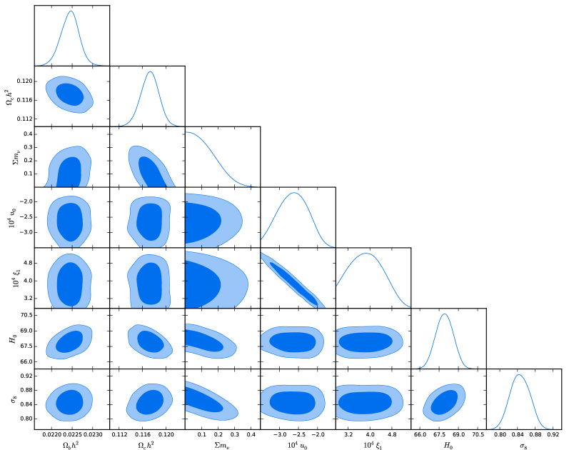
Figure 1: One and two-dimensional distributions of $\Omega_{b}h^{2}$, $\Omega_{c}h^{2}$, $\sum m_{\nu}$, $10^{4}u_{0}$, $10^{4}\xi_{1}$, $H_{0}$, and $\sigma_{8}$ for $\Lambda(\alpha)$CDM1 with ${\xi(a)}=3+u_{0}+\xi_{1}(1-a)$, where the contour lines represent 68$\%$  and 95$\%$  C.L., respectively.

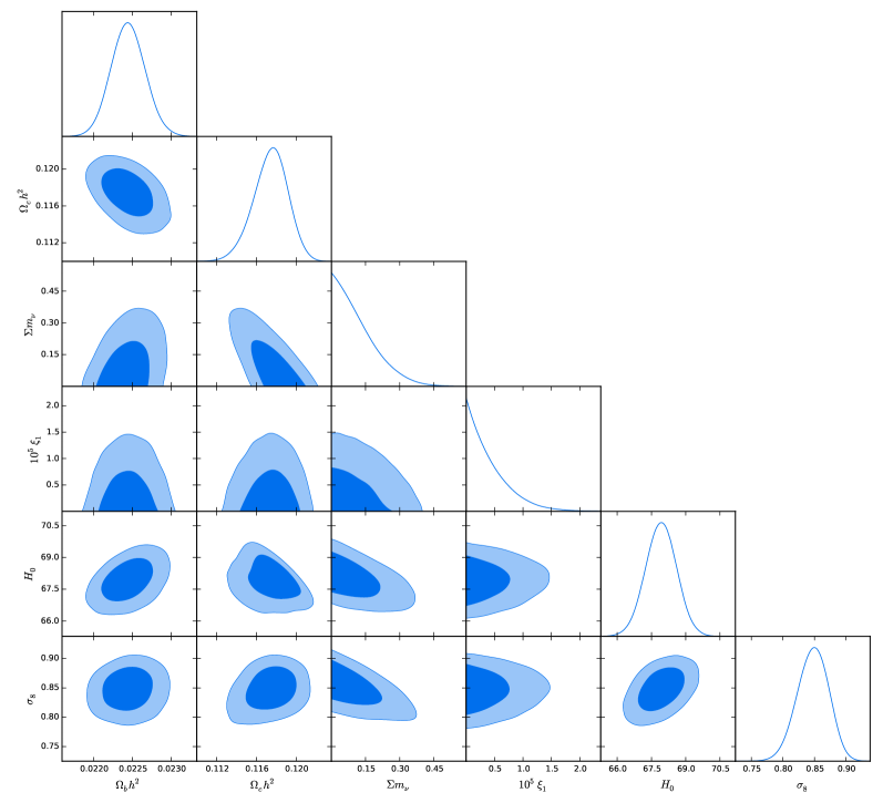
Figure 2: Legend is the same as Fig. 1 but for $\Lambda(\alpha)$CDM2 with ${\xi(a)}=3+\xi_{1}(1-a)$.

We summarize our fitting results for the two $\Lambda(\alpha)$CDM models in Table 2, in which we also include those in $\Lambda$CDM. It is clear that the model parameters of $u_{0}$ and $\xi_{1}$ in the $\Lambda(\alpha)$CDM models are zero in the limit of $\Lambda$CDM.

Table 2: Summary of the fitting results for $\Lambda(\alpha)$CDM1 with ${\xi(a)}=3+u_{0}+\xi_{1}(1-a)$ and $\Lambda(\alpha)$CDM2 with ${\xi(a)}=3+\xi_{1}(1-a)$ as well as those for $\Lambda$CDM, where 313 $\Delta\alpha/\alpha$ data are used the limits are given at 68$\%$ C.L.

Model	$100\Omega_{b}h^{2}$	$100\Omega_{c}h^{2}$	$H_{0}$	$\sigma_{8}$	${\Sigma m_{\nu}\over\mathrm{eV}}$	$10^{4}u_{0}$	$10^{4}\xi_{1}$	$\chi^{2}_{best-fit}$
$\Lambda(\alpha)$CDM1	$2.24\pm 0.02$	$11.7^{+0.16}_{-0.14}$	$67.90\pm 0.69$	$0.844^{+0.027}_{-0.023}$	$0.123^{+0.032}_{-0.122}$	$-2.67^{+0.39}_{-0.40}$	$3.95^{+0.59}_{-0.64}$	$1844.132$
$\Lambda(\alpha)$CDM2	$2.24\pm 0.02$	$11.7^{+0.19}_{-0.15}$	$67.91^{+0.71}_{-0.68}$	$0.847^{+0.028}_{-0.025}$	$<0.144$	$-$	$0.0409^{+0.0080}_{-0.0409}$	$1870.837$
$\Lambda$CDM	$2.25\pm 0.02$	$11.7^{+0.20}_{-0.16}$	$67.83^{+0.74}_{-0.67}$	$0.843^{+0.027}_{-0.024}$	$<0.165$	$0$	$0$	$1869.854$

From the table, we find that $u_{0}=(-2.667^{+0.393}_{-0.398})\times 10^{-4}$ and $\xi_{1}=(3.953^{+0.591}_{-0.641})\times 10^{-4}$ in ${\xi(a)}=3+u_{0}+\xi_{1}(1-a)$ of $\Lambda(\alpha)$CDM1 and $0.409^{+0.080}_{-0.409}\times 10^{-5}$ in ${\xi(a)}=3+\xi_{1}(1-a)$ of $\Lambda(\alpha)$CDM2 with the best fitted $\chi^{2}$ values being $1844.132$ and $1870.837$, respectively. As expected, the two-parameter model of $\Lambda(\alpha)$CDM1 gives the lowest value of $\chi^{2}_{bestfit}$, while the one-parameter one of $\Lambda(\alpha)$CDM1 leads to a slightly larger $\chi^{2}_{bestfit}$ than $\Lambda$CDM. The lower bound of $\xi_{1}$ in $\Lambda(\alpha)$CDM2 is due to its prior set from zero in Table 1. Without such a prior, a negative value at $O(10^{-5})$ for $\xi_{1}$ is also possible. It is clear that our fitting results for $\Lambda(\alpha)$CDM1 with two free model parameters are better than those for $\Lambda(\alpha)$CDM2 with a single one. Comparing with the best-fit values $u_{0}$ and $\xi_{1}$ in $\Lambda(\alpha)$CDM1 given by Ref. Wei:2016moy , our results are slightly different due to the different fitting method and cosmological data in our calculations.

From Table 2, it is interesting to see that our fitting result for ${\Sigma m_{\nu}}$ in $\Lambda(\alpha)$CDM1 is $0.123^{+0.032}_{-0.122}$ eV at $68\%$ C.L., whereas that for $\Lambda(\alpha)$CDM2 only gives the upper bound of $0.152$ eV. We note that the values of $\sigma_{8}$ in our two models are both slightly larger that that in $\Lambda$CDM.

To understand the behaviors of ${\Sigma m_{\nu}}$ in the various models, we show the matter power spectra as functions of the wavelength $k=2\pi/\lambda$ in the $\Lambda$CDM as well as $\Lambda(\alpha)$CDM1 and $\Lambda(\alpha)$CDM2 models in Fig. 3.

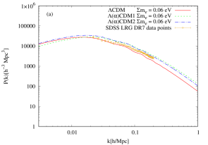
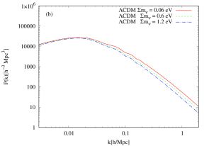
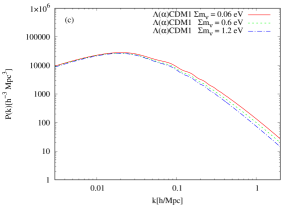
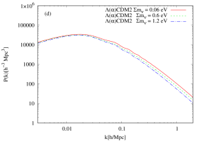
Figure 3: Matter power spectra of $P(k)$ as functions of the wavelength $k=2\pi/\lambda$ in (a) $\Lambda(\alpha)$CDM and $\Lambda$CDM with $\Sigma m_{\nu}$=0.06 eV along with the observational data, (b) $\Lambda$CDM with $\Sigma m_{\nu}$=0.06, 0.6 and 1.2 eV, (c) $\Lambda(\alpha)$CDM1 with $\Sigma m_{\nu}$=0.06, 0.6 and 1.2 eV, and (d) $\Lambda(\alpha)$CDM2 with $\Sigma m_{\nu}$=0.06, 0.6 and 1.2 eV.

To exhibit the trend of the matter power spectrum in terms of $\Sigma m_{\nu}$, we present Figs. 3b, 3c and 3d for $\Lambda$CDM, $\Lambda(\alpha)$CDM1 and $\Lambda(\alpha)$CDM2 with $\Sigma m_{\nu}$=0.06, 0.6 and 1.2 eV, respectively. From Fig. 3a with the fixed value of $\Sigma m_{\nu}=0.06$ eV, we find that, in comparison with $\Lambda$CDM, the matter power spectrum in $\Lambda(\alpha)$CDM1(2) gets enhanced for the most (all) region of $k$, whereas that in $\Lambda(\alpha)$CDM1 slightly suppressed for the low values of $k$. On the other hand, the value of $\Sigma m_{\nu}$ increases the suppression factor for the matter power spectrum within the same model as illustrated in Figs. 3b-d. The enhancement behaviors of the matter power spectra in $\Lambda(\alpha)$CDM are similar to the cases in the viable $f(R)$ gravity models as studied in Ref. f(R)NuMass . In Fig. 4, we depict our results of $\Lambda(\alpha)$CDM2 for chains with $\Sigma m_{\nu}$ fixed to be 0.06 eV to illustrate the best-fit parameters.

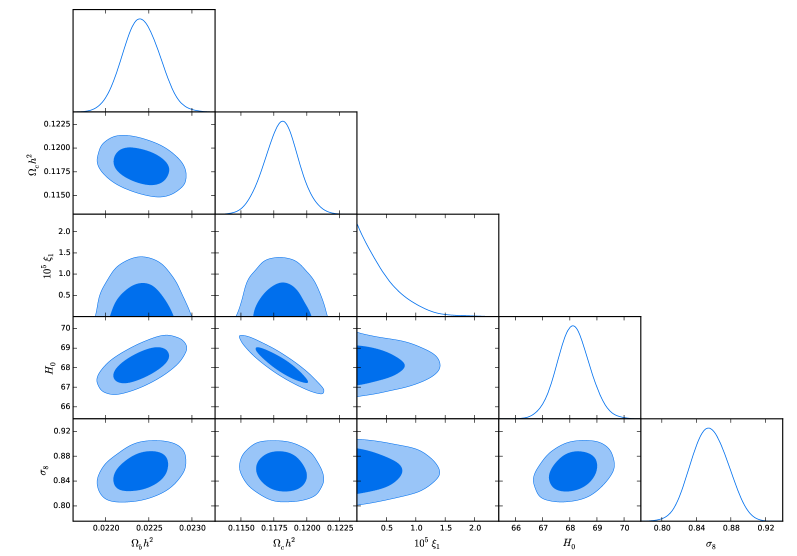
Figure 4: One and two-dimensional distributions of $\Omega_{b}h^{2}$, $\Omega_{c}h^{2}$, $10^{5}\xi_{1}$, $H_{0}$, and $\sigma_{8}$ for $\Lambda(\alpha)$CDM2 with ${\xi(a)}=3+\xi_{1}(1-a)$ with $\Sigma m_{\nu}$=0.06 eV, where the contour lines represent 68% and 95% C.L., respectively.

We also summary our fit for $\Lambda(\alpha)$CDM2 $\Sigma m_{\nu}=0.06$ eV in Table 3, where the corresponding results for $\Lambda$CDM are also given.

Table 3: Summary of the fitting results for $\Lambda(\alpha)$CDM2 with ${\xi(a)}=3+\xi_{1}(1-a)$ and ${\Sigma m_{\nu}=0.06\mathrm{eV}}$, the limits are given at 68$\%$ C.L.

Model	$100\Omega_{b}h^{2}$	$100\Omega_{c}h^{2}$	$H_{0}$	$\sigma_{8}$	$10^{5}\xi_{1}$	$\chi^{2}_{best-fit}$
$\Lambda(\alpha)$CDM2	$2.24\pm 0.02$	$11.8\pm 0.1$	$68.11^{+0.59}_{-0.60}$	$0.853\pm 0.021$	$0.418^{+0.089}_{-0.418}$	$1872.230$
$\Lambda$CDM	$2.24\pm 0.02$	$11.8\pm 0.1$	$68.13^{+0.59}_{-0.60}$	$0.855^{+0.019}_{-0.022}$	$0$	$1870.574$

Note that we are able to get a good fit for $\Lambda(\alpha)$CDM1 with $\Sigma m_{\nu}\sim 0$ as it favors a large $\Sigma m_{\nu}$ as indicated in Table 2. It is interesting to see that the best-fit value of $\chi^{2}$ for $\Lambda(\alpha)$CDM2 with $m_{\nu}$ fixed to be 0.06 eV is 1872.230, which is larger than 1870.837 without fixing $m_{\nu}$. Note that the corresponding values of $\chi^{2}_{best-fit}$ are 1870.574 and 1869.854 for $\Lambda$CDM with and without fixed $m_{\nu}$, respectively.

Finally, we remark that the model parameter of $\xi_{1}$ can be also constrained directly by using Eq. (19). For example, one can show that $\xi_{1}$ in $\Lambda(\alpha)$CDM is $O(10^{-4})$ for ${\Delta\alpha}/{\alpha}=\mathcal{O}(10^{-5})$.

IV Conclusions

We have studied the $\Lambda(\alpha)$CDM models with $\Lambda(\alpha)\propto\alpha^{-6}$, in which the fine structure constant $\alpha$ varies in time with the data of ${\Delta\alpha}/{\alpha}=\mathcal{O}(10^{-5})$. In particular, we have concentrated on two specific $\Lambda(\alpha)$CDM models in Eqs. (18) and (20) with two and one model parameters, respectively. We have performed global fits on the two models by using the available cosmological data in the CAMB and CosmoMC packages together with 313 data points for ${\Delta\alpha}/{\alpha}$ from distant quasars. We have shown that the model parameters are constrained to be around $10^{-4}$, which are similar to those given by Ref.  Wei:2016moy but with more accurate outcomes. For $\Lambda(\alpha)$CDM1, we have derived an interesting fitting value of ${\Sigma m_{\nu}}$ is $0.123^{+0.032}_{-0.122}$eV, which gives not only an upper bound of 0.155 eV but a lower one of $9.87\times 10^{-4}$ eV, instead of the only upper bounds in most of cosmological models, including $\Lambda$CDM and $\Lambda(\alpha)$CDM2. In addition, we have found that the best fitted $\chi^{2}$ values are 1844.132 and 1870.837 for the two models of $\Lambda(\alpha)$CDM1 and $\Lambda(\alpha)$CDM2, respectively.

References

• (1) A. Einstein, Sitzungsber. Preuss. Akad. Wiss. Berlin (Math. Phys. ) 1917, 142 (1917).
• (2) C. O’Raifeartaigh, M. O’Keeffe, W. Nahm and S. Mitton, arXiv:1711.06890 [physics.hist-ph].
• (3) P. J. E. Peebles and B. Ratra, Rev. Mod. Phys.  75, 559 (2003).
• (4) A. G. Riess et al. [Supernova Search Team], Astron. J.  116, 1009 (1998).
• (5) S. Perlmutter et al. [Supernova Cosmology Project Collaboration], Astrophys. J.  517, 565 (1999).
• (6) J. P. Ostriker and P. J. Steinhardt, astro-ph/9505066.
• (7) N. Arkani-Hamed, L. J. Hall, C. F. Kolda and H. Murayama, Phys. Rev. Lett.  85, 4434 (2000).
• (8) S. Weinberg, Rev. Mod. Phys.  61, 1 (1989).
• (9) S. Weinberg, Gravitation and Cosmology, (Wiley and Sons, New York, 1972).
• (10) L. Amendola and S. Tsujikawa, Dark Energy Theory and Observations, (Cambridge University Press, Cambridge, 2010).
• (11) C. Beck, Physica A 388, 3384 (2009).
• (12) A. I. Khinchin, Mathematical Foundations of Information Theory, Dover Publications, New York (1957).
• (13) C. G. Boehmer and T. Harko, Phys. Lett. B 630, 73 (2005).
• (14) P. S. Wesson, Mod. Phys. Lett. A 19, 1995 (2004).
• (15) C. G. Boehmer and T. Harko, Found. Phys.  38, 216 (2008).
• (16) A. Eddington, Proc. Camb. Philos. Soc. 27, 15 (1931); Relativity Theory of Proton and Electrons, Cambridge University Press (1936).
• (17) P. A. M. Dirac, Nature 139, 323 (1937).
• (18) H. Weyl, Ann. Physik 59, 129 (1919).
• (19) L. Nottale, Mach’s Principle, Dirac’s Large Numbers, and the Cosmological Constant Problem, preprint (1993).
• (20) H. Wei, X. B. Zou, H. Y. Li and D. Z. Xue, Eur. Phys. J. C77, 14 (2017).
• (21) J. K. Webb, V. V. Flambaum, C. W. Churchill, M. J. Drinkwater and J. D. Barrow, Phys. Rev. Lett.  82, 884 (1999).
• (22) J. K. Webb, M. T. Murphy, V. V. Flambaum, V. A. Dzuba, J. D. Barrow, C. W. Churchill, J. X. Prochaska and A. M. Wolfe, Phys. Rev. Lett.  87, 091301 (2001).
• (23) J. A. King, J. K. Webb, M. T. Murphy, V. V. Flambaum, R. F. Carswell, M. B. Bainbridge, M. R. Wilczynska and F. E. Koch, Mon. Not. Roy. Astron. Soc.  422, 3370 (2012).
• (24) J. K. Webb, J. A. King, M. T. Murphy, V. V. Flambaum, R. F. Carswell and M. B. Bainbridge, Phys. Rev. Lett.  107, 191101 (2011).
• (25) J. P. Uzan, Living Rev. Rel.  14, 2 (2011).
• (26) H. Wei, Phys. Lett. B 682, 98 (2009).
• (27) H. Wei, X. P. Ma and H. Y. Qi, Phys. Lett. B 703, 74 (2011).
• (28) H. Terazawa, Nonlin. Phenom. Complex Syst.  20, 241 (2014).
• (29) H. Terazawa, Phys. Lett. B 101, 43 (1981).
• (30) M. T. Murphy, J. K. Webb, V. V. Flambaum, V. A. Dzuba, C. W. Churchill, J. X. Prochaska, J. D. Barrow and A. M. Wolfe, Mon. Not. Roy. Astron. Soc.  327, 1208 (2001).
• (31) A. Lewis, A. Challinor and A. Lasenby, Astrophys. J.  538, 473 (2000) [astro-ph/9911177].
• (32) A. Lewis and S. Bridle, Phys. Rev. D 66, 103511 (2002).
• (33) http://astronomy.swin.edu.au/ mmurphy/files/KingJ.12a.VLT+Keck.dat
• (34) http://mnras.oxfordjournals.org/content/422/4/3370/suppl/DC1
• (35) http://mnras.oxfordjournals.org/content/suppl/2013/01/17/j.1365-2966.2012.20852.x.DC1/mnras0422- 3370-SD1.txt
• (36) M. R. Wilczynska, J. K. Webb, J. A. King, M. T. Murphy, M. B. Bainbridge and V. V. Flambaum, Mon. Not. Roy. Astron. Soc.  454, no. 3, 3082 (2015) doi:10.1093/mnras/stv2148 [arXiv:1510.02536 [astro-ph.CO]].
• (37) R. G. Cai, L. M. Cao and N. Ohta, Phys. Rev. D 81, 061501 (2010) doi:10.1103/PhysRevD.81.061501 [arXiv:1001.3470 [hep-th]].
• (38) N. Dalal, K. Abazajian, E. E. Jenkins and A. V. Manohar, Phys. Rev. Lett.  87, 141302 (2001).
• (39) Z. K. Guo, N. Ohta and S. Tsujikawa, Phys. Rev. D 76, 023508 (2007).
• (40) H. Wei, Phys. Lett. B 691, 173 (2010).
• (41) M. Chevallier and D. Polarski, Int. J. Mod. Phys. D 10, 213 (2001); E. V. Linder, Phys. Rev. Lett.  90, 091301 (2003).
• (42) C. P. Ma and E. Bertschinger, Astrophys. J.  455, 7 (1995).
• (43) J. Grande, A. Pelinson and J. Sola, Phys. Rev. D 79, 043006 (2009) doi:10.1103/PhysRevD.79.043006 [arXiv:0809.3462 [astro-ph]].
• (44) A. G mez-Valent and J. Sol , arXiv:1801.08501 [astro-ph.CO].
• (45) Y. Wang, D. Wands, G. B. Zhao and L. Xu, Phys. Rev. D 90, no. 2, 023502 (2014) doi:10.1103/PhysRevD.90.023502 [arXiv:1404.5706 [astro-ph.CO]].
• (46) Y. Wang, D. Wands, L. Xu, J. De-Santiago and A. Hojjati, Phys. Rev. D 87, no. 8, 083503 (2013) doi:10.1103/PhysRevD.87.083503 [arXiv:1301.5315 [astro-ph.CO]].
• (47) R. Adam et al. [Planck Collaboration], Astron. Astrophys.  594, A10 (2016).
• (48) N. Aghanim et al. [Planck Collaboration], Astron. Astrophys.  594, A11 (2016).
• (49) P. A. R. Ade et al. [Planck Collaboration], Astron. Astrophys.  594, A15 (2016).
• (50) C. Heymans et al., Mon. Not. Roy. Astron. Soc.  432, 2433 (2013).
• (51) F. Beutler et al., Mon. Not. Roy. Astron. Soc.  416, 3017 (2011).
• (52) L. Anderson et al. [BOSS Collaboration], Mon. Not. Roy. Astron. Soc.  441, 24 (2014).
• (53) G. Bazin et al., Astron. Astrophys.  534, A43 (2011).
• (54) C. Q. Geng, C. C. Lee and J. L. Shen, Phys. Lett. B 740, 285 (2015).