Gyrokinetic simulation of ITG turbulence with toroidal geometry including the magnetic axis by using field-aligned coordinates

Abstract

Simulation domain in field-aligned coordinates of the electrostatic gyrokinetic nonlinear turbulence global code, NLT, is extended to include the magnetic axis. The artificial boundary near the magnetic axis is replaced by the natural boundary. The singularity at the magnetic axis in Vlasov solver is treated by considering the spatial relation of fixed grid points in field-aligned coordinates. A new Poisson’s equation solver is developed, the coefficient matrix of algebraic equations is derived by using Gauss’s theorem. Nonlinear relaxation test of the ITG turbulence with adiabatic electrons is performed. The gyrocenter conservation is much improved by including the magnetic axis in the simulation domain. The zonal field and the radial distribution of the perturbed electrostatic potential are different from previous results without the magnetic axis.

1 Introduction

Gyrokinetic simulation is an important tool for investigating properties of the low frequency turbulence in magnetized plasmas[1]. In a tokamak, the low frequency drift wave turbulence and the guiding center drift motion are inseparable, 3D toroidal geometry is necessary for gyrokinetic simulation. There are two kinds of space domain selection in gyrokinetic simulation with 3D toroidal geometry. One is the flux-tube domain[2, 3]. This domain is several correlation lengths wide in both radial and poloidal directions and extended along the field line. Flux-tube simulations require less computational cost. But the zonal field in the simulation domain cannot be evolved self-consistently, and researchers have realized that the zonal field plays an important role in turbulence nonlinear saturation[4, 5]. The other one is the global domain[4, 6, 7]. It includes most space in a tokamak. The self-consistent evolution of the zonal field is involved in global simulations. The computational cost of a global simulation is much more then that of a flux-tube simulation. With the development of computers, global simulations have been widely used in research of tokamak plasma physics.

However, the magnetic axis is not included in most global simulations[7, 8, 9, 10]. Usually, the artificial internal boundary in radial direction is used. This artificial boundary have an influence on field solver, guiding center motion and system conservation, which makes some simulation results difficult to grasp. Recently, in order to prevent particles from escaping the computational domain, researchers improve the radial boundaries of GYSELA code[11], but the magnetic axis is still not included in simulation and the internal radial boundary still exist. A new finite element field solver is used in GTC to extend the simulation domain including the magnetic axis[12], but a zero boundary condition at both inner and outer boundaries is imposed in this new field solver. Difficulty of simulation at the magnetic axis region mainly comes from the 3D toroidal geometry. Many equilibrium quantities are functions of the poloidal magnetic flux. Thus, it is natural to use magnetic coordinates (magnetic flux coordinates or field-aligned coordinates) in global simulation. Magnetic coordinates are generalized polar coordinates in the radial-poloidal plane. In equations of motion, the velocity of poloidal angular coordinate is singular at the magnetic axis[13].

The magnetic axis is included in the simulation domain of the PIC code ORB5[14, 15, 13] and the Eulerian code GT5D[16]. The finite element approach is used by these two codes to solve the Poisson’s equation[17, 18, 19], a natural boundary condition is imposed at the magnetic axis. In ORB5, in order to avoid the singularity at the magnetic axis, it is adequate to use the equivalent cylindrical coordinates, and equilibrium coefficients needed for the pushing are obtained with linear interpolations[13]. And also, the Vlasov solver of the GT5D is treated in cylindrical coordinates, thus a mapping between cylindrical coordinates and magnetic flux coordinates is used in the simulation[16].

In this paper, the numerical method to treat the magnetic axis in the electrostatic gyrokinetic nonlinear turbulence global code, NLT, by using field-aligned coordinates is presented. NLT is a continuum code based on the numerical Lie transform method[20, 21]. The key idea of the numerical Lie transform method is to decouple the perturbed motion of the gyrocenter from the unperturbed motion, and the perturbed distribution function is obtained from the unperturbed one by using pull-back transform[22, 23, 24, 25]. NLT is mainly composed of four parts: integration along the unperturbed orbit, pull-back transform, Poisson’s equation solver and numerical filter. Special numerical schemes are adopted in all these parts at the magnetic axis. The remaining part of this paper is organized as follows. In Sec. 2, the fundamental equations are introduced, the previous numerical schemes in NLT and its limitation at the magnetic axis are reviewed. Sec. 3, computation of the unperturbed guiding center orbit. Sec. 4, numerical scheme of pull-back transform at the magnetic axis. Sec. 5, a new Poisson’s equation solver is described. Sec. 6, numerical filter. Sec. 7, nonlinear relaxation test. Sec. 8, summary and discussion.

2 Review of the NLT code

In this section, the fundamental equations are introduced firstly. Then the previous numerical schemes in NLT and its limitation at the magnetic axis are reviewed.

2.1 Fundamental equations

The gyrocenter distribution function $F\left(\bm{Z}\right)$ satisfies the gyrokinetic Vlasov equation

$$\frac{\mathrm{d}F}{\mathrm{d}t}\equiv\partial_{t}F+\dot{\bm{X}}\cdot\nabla F+\dot{V}_{\parallel}\partial_{V_{\parallel}}F=0,$$ (1)

where $\bm{Z}=\left(\bm{X},V_{\parallel},\mu\right)$, and $V_{\parallel}$ is the parallel velocity, $\mu$ is the magnetic moment, $\bm{X}$ is the position of the gyro-center. The gyrokinetic quasi-neutrality equation in the long-wavelength approximation with adiabatic electron is[26]

$$\nabla\cdot\left(c_{0}\nabla_{\perp}\phi\right)-c_{1}\left(\phi-\left\langle\phi\right\rangle_{FA}\right)=c_{2}\rho_{i,gy}.$$ (2)

with $c_{0}=\frac{n_{0i}m_{i}}{B^{2}}$, $c_{1}=\frac{e^{2}n_{0e}}{T_{e}}$, $c_{2}=-e_{i}$. Here $n_{0i}$ and $n_{0e}$ represent the equilibrium density of ion and electron, respectively, $m_{i}$ is the mass of ion, $B$ is the equilibrium magnetic field, $T_{e}$ is the temperature of electron, $e$ and $e_{i}$ respectively represent electric charge of electron and ion. $\rho_{i,gy}$ is the gyrocenter density of the ion, which is given by

$$\rho_{i,gy}=\int\mathrm{d}V_{\parallel}\mathrm{d}\mu 2\pi B_{\parallel}^{*}\left\langle\delta F\right\rangle_{GA},$$ (3)

with

$$B_{\parallel}^{*}=B+\frac{m_{i}V_{\parallel}}{e_{i}}\bm{b}\cdot\nabla\times\bm{b},$$ (4)

$\bm{b}=\frac{\bm{B}}{B}$. The gyro-average operator $\left\langle\cdot\right\rangle_{GA}$ is defined as

$$\left\langle f\right\rangle_{GA}\left(\bm{r},\mu\right)\equiv\frac{1}{2\pi}\int_{0}^{2\pi}f\left(\bm{X}+\bm{\rho}\left(\mu,\xi\right)-\bm{r}\right)\mathrm{d}\xi,$$ (5)

$\left\langle\phi\right\rangle_{FA}$ represents the magnetic surface averaged electrostatic potential. The magnetic surface averaged operator $\left\langle\cdot\right\rangle_{FA}$ is defined as

$$\left\langle f\right\rangle_{FA}\equiv\frac{\int_{0}^{2\pi}\mathrm{d}\alpha\int_{0}^{2\pi}\mathrm{d}\theta J_{\bm{X}}f}{\int_{0}^{2\pi}\mathrm{d}\alpha\int_{0}^{2\pi}\mathrm{d}\theta J_{\bm{X}}},$$ (6)

with $J_{\bm{X}}$ being the space Jacobian.

The equilibrium magnetic field can be expressed in terms of magnetic flux coordinates $\bm{X}_{f}\equiv(\psi^{*},\theta^{*},\zeta^{*})$ as

$$\bm{B}=g\left(\psi^{*}\right)\nabla\zeta^{*}+I\left(\psi^{*}\right)\nabla\theta^{*}+g\left(\psi^{*}\right)\delta\left(\psi^{*},\theta^{*}\right)\nabla\psi^{*},$$ (7)

where $\psi^{*}$ is the poloidal magnetic flux, $\theta^{*}$ is the poloidal angle, $\zeta^{*}$ is the toroidal angle. $I\left(\psi^{*}\right)$ and $g\left(\psi^{*}\right)$ represent the toroidal and poloidal components of the magnetic field in the covariant form, respectively. For micro-turbulence in tokamak plasmas, the perpendicular wavenumber is much larger then the parallel wavenumber, $k_{\perp}\gg k_{\parallel}$. Therefore, field-aligned coordinates $\bm{X}_{l}\equiv(\psi,\theta,\alpha)$ can be used to improve the computational efficiency, where

$$\psi=\psi^{*},$$ (8)

$$\theta=\theta^{*},$$ (9)

$$\alpha=q\left(\psi^{*}\right)\theta^{*}-\zeta^{*},$$ (10)

$q\left(\psi^{*}\right)$ is the safety factor. The space Jacobian is

$$J_{\bm{X}}\equiv J_{\psi,\theta,\alpha}=J_{\psi^{*},\theta^{*},\zeta^{*}}=\frac{gq+I}{B^{2}}.$$ (11)

For convenience, $\bm{Z}\equiv\left(\bm{X}_{l},V_{\parallel},\mu\right)$ in the rest part of this paper.

2.2 Numerical algorithm

Unlike traditional continuum methods, the process of solving the Vlasov equation in numerical Lie transform is divided into $2$ sub-processes, the unperturbed solver and the perturbed solver[22, 23]. The unperturbed solver is treated by integrating along the unperturbed orbit. The perturbed solver is treated by pull-back transform, which is equivalent to compute the perturbed orbit. Thus, NLT is mainly composed of $4$ parts: integration along the unperturbed orbit, pull-back transform, Poisson’s equation solver and numerical filter.

In the first part, $\delta\bar{F}$ and $S_{1}$ are computed[20], the former represents the evolution of the perturbed distribution function $\delta F$ under the equilibrium field, the latter represents the gauge function of the I-transform[22, 23],

$$\frac{\mathrm{d}_{0}}{\mathrm{d}t}\delta\bar{F}=0,$$ (12)

$$\frac{\mathrm{d}_{0}}{\mathrm{d}t}S_{1}=e_{i}\left\langle\phi\right\rangle_{GA},$$ (13)

the total time derivative $\frac{\mathrm{d}_{0}}{\mathrm{d}t}$ is taken along the unperturbed orbit. At the beginning of each time step, $S_{1}=0$, $\delta\bar{F}=\delta F$. Numerically, we can obtain the solution by using the semi-Lagrangian method and the high dimensional fixed point interpolation algorithm[27],

$$\delta\bar{F}\left(\bm{Z},t+\Delta t\right)=\delta\bar{F}\left(\bm{Z}+\Delta\bm{Z}_{0}\left(-\Delta t\right),t\right)=\delta F\left(\bm{Z}+\Delta\bm{Z}_{0}\left(-\Delta t\right),t\right),$$ (14)

$$S_{1}\left(\bm{Z},t+\Delta t\right)=e_{i}\int_{t}^{t+\Delta t}\left\langle\phi\right\rangle_{GA}\left(\bm{Z}+\Delta\bm{Z}_{0}\left(t-\tau\right),\tau\right)\mathrm{d}\tau,$$ (15)

where

$$\Delta\bm{Z}_{0}\left(t\right)\equiv\int_{0}^{t}\left\{\bm{Z},H_{0}\right\}\mathrm{d}t,$$ (16)

$H_{0}$ is the unperturbed guiding center Hamiltonian,

$$H_{0}=\frac{1}{2}mV_{\parallel}^{2}+\mu B,$$ (17)

$\{\text{},\text{}\}$ is the Poisson bracket,

$$\left\{f,g\right\}=\frac{\partial f}{\partial Z^{a}}J^{Z^{a}Z^{b}}\frac{\partial g}{\partial Z^{b}},$$ (18)

$J^{Z^{a}Z^{b}}$ is the component of the unperturbed Poisson matrix, which can be expressed as[21]

$$J^{\psi\theta}=-J^{\theta\psi}=J^{\psi^{*}\theta^{*}},$$ (19)

$$J^{\psi\alpha}=-J^{\alpha\psi}=qJ^{\psi^{*}\theta^{*}}-J^{\psi^{*}\zeta^{*}},$$ (20)

$$J^{\psi V_{\parallel}}=-J^{V_{\parallel}\psi}=J^{\psi^{*}V_{\parallel}},$$ (21)

$$J^{\theta\alpha}=-J^{\alpha\theta}=-J^{\theta^{*}\zeta^{*}}-q^{\prime}\theta J^{\psi^{*}\theta^{*}},$$ (22)

$$J^{\theta V_{\parallel}}=-J^{V_{\parallel}\theta}=J^{\theta^{*}V_{\parallel}},$$ (23)

$$J^{\alpha V_{\parallel}}=-J^{V_{\parallel}\alpha}=qJ^{\theta^{*}V_{\parallel}}+q^{\prime}\theta J^{\psi^{*}V_{\parallel}}-J^{\zeta^{*}V_{\parallel}},$$ (24)

with $J^{Z_{f}^{a}Z_{f}^{b}}$ the form of the unperturbed Poisson matrix component in $\bm{Z}_{f}\equiv\left(\bm{X}_{f},V_{\parallel},\mu\right)$

$$J^{\psi^{*}\theta^{*}}=-\frac{g}{e_{i}D},$$ (25)

$$J^{\psi^{*}\zeta^{*}}=\frac{I}{e_{i}D},$$ (26)

$$J^{\psi^{*}V_{\parallel}}=\frac{V_{\parallel}B}{e_{i}D}\partial_{\theta^{*}}\left(\frac{g}{B}\right),$$ (27)

$$J^{\theta^{*}\zeta^{*}}=\frac{g\delta}{e_{i}D},$$ (28)

$$J^{\theta^{*}V_{\parallel}}=-J^{V_{\parallel}\theta}=\frac{B}{m_{i}D}\left[1-\frac{m_{i}V_{\parallel}}{e_{i}}\partial_{\psi^{*}}\left(\frac{g}{B}\right)\right],$$ (29)

$$J^{\zeta^{*}V_{\parallel}}=\frac{B}{m_{i}D}\left\{q+\frac{m_{i}V_{\parallel}}{e_{i}}\left[\partial_{\psi^{*}}\left(\frac{I}{B}\right)+\partial_{\theta^{*}}\left(\frac{g\delta}{B}\right)\right]\right\},$$ (30)

$$q^{\prime}=\frac{\mathrm{d}q}{\mathrm{d}\psi^{*}},$$ (31)

$$D=qg+I+\rho_{\parallel}\left(I^{\prime}g-g^{\prime}I\right)-\rho_{\parallel}g^{2}\partial_{\theta^{*}}\delta,$$ (32)

$$\rho_{\parallel}=\frac{m_{i}V_{\parallel}}{e_{i}B}.$$ (33)

Usually, in the region away from the magnetic axis, $J^{\theta V_{\parallel}}\approx\frac{B}{m_{i}D}$. However, in the region near the magnetic axis, when $\psi\to 0$, $J^{\theta V_{\parallel}}\approx\frac{BV_{\parallel}}{De_{i}}\partial_{\psi}\left(\frac{g}{B}\right)\propto r^{-1}$, where $r$ is the minor radius. $J^{\theta V_{\parallel}}$ contributes the velocity of guilding center in $V_{\parallel}$ and $\theta$ directions. The contribution in $V_{\parallel}$ direction is $-J^{\theta V_{\parallel}}\partial_{\theta}H_{0}$, near the magnetic axis, $\partial_{\theta}H_{0}\propto r$, thus this contribution is not divergent, but it is difficult to be treated numerically. The contribution in $\theta$ direction is $J^{\theta V_{\parallel}}\partial_{V_{\parallel}}H_{0}=V_{\parallel}J^{\theta V_{\parallel}}$, it is divergent; as is mentioned in the introduction, this singularity is due to the properties of the generalized polar coordinates.

In the second part, $\delta F$ is computed by using pull-back transform[21]

$$\delta F=\delta\bar{F}+\delta F_{A}+\delta F_{B},$$ (34)

$$\delta F_{A}=G_{1}^{Z^{a}}\frac{\partial}{\partial Z^{a}}\left(F_{0}+\delta\bar{F}\right),$$ (35)

$$\delta F_{B}=\frac{1}{2}G_{1}^{Z^{a}}\frac{\partial}{\partial Z^{a}}\delta F_{A},$$ (36)

where $\bm{G}_{1}$ is the 1st order generating vector field,

$$\bm{G}_{1}=\left\{S_{1},\bm{Z}\right\}.$$ (37)

The main task of this part is to compute numerical differentiations. Note that the Poisson matrix is needed for computing $\bm{G}_{1}$, the singularity will also appear at the magnetic axis. Considering that the pull-back transform is equivalent to the computation of the perturbed orbit, the problem and the solution of this singularity are same as that in the first part.

The gyrokinetic quasi-neutrality equation is solved in the third part[21]. $\left\langle\phi\right\rangle_{FA}$ is solved approximately from the equation by taking the magnetic surface average on both sides of the Eq. (2). The partial differential operator in $\alpha$ direction is converted to algebraic operator by the toroidal Fourier transform. Further, by considering that the $\theta$ direction is parallel to the magnetic field line in field-aligned coordinates and $k_{\perp}\gg k_{\parallel}$, we regard the term containing $\partial_{\theta}$ as a correction in numerical, which can be computed iteratively. Thus, the three-dimensional second-order partial differential operators reduced to one-dimensional second-order differential operators. In numerical, $\phi$ is solved iteratively by using the finite difference method with the Dirichlet boundary conditions.

There are three shortcomings in this field solver. First, $\left\langle\phi\right\rangle_{FA}$ is an approximate solution; Second, the Dirichlet boundary condition at the inner boundary is not self-consistent; Third, at the magnetic axis, $\partial_{\theta}=-q\partial_{\alpha}$, thus the term containing $\partial_{\theta}$ cannot be treated as a correction in numerical.

The last part is the numerical filter. The Fourier filter, zeroing the coefficients of Fourier components with wavelengths of these components being less than three times the width of the grid, is adopted in NLT[21]. The phase-space density function $J_{\bm{Z}}\delta F$ is filtered in each time step, where $J_{\bm{Z}}$ is the phase-space Jacobian. Note that $\delta F$ is very small near the computational velocity boundary and the damping buffer regions are used near the radial boundaries, the Gibbs phenomenon has a less impact on the simulation. Thus, although the boundary conditions in both $\psi$ and $V_{\parallel}$ directions are not periodic, the Fourier filter is still used in these directions. Considering that $\theta$ is also non-periodic in the field-aligned coordinates, we transform $J_{\bm{Z}}\delta F$ from field-aligned coordinates into magnetic flux coordinates$J_{\bm{Z}_{f}}\delta F_{f}$ to truncate the shortwave in the parallel direction by using the Fourier filter, with $J_{\bm{Z}_{f}}$ the phase-space Jacobian of $\bm{Z}_{f}$. $\left(J_{\bm{Z}_{f}}\delta F_{f}\right)_{mn}$ is the Fourier component of $J_{\bm{Z}_{f}}\delta F_{f}$, $n$ and $m$ are the mode number in $\zeta^{*}$ and $\theta^{*}$ directions, respectively. Filter conditions are determined by fixed grid points in field-aligned coordinates, $\left(J_{\bm{Z}_{f}}\delta F_{f}\right)_{mn}=0$ when $n>N_{\alpha}/3$, $m<nq-N_{\theta}/3$ or $m\text{>}nq+N_{\theta}/3$, where $N_{\theta}$ and $N_{\alpha}$ are the total number of grid points in the $\theta$ and $\alpha$ directions.

If the magnetic axis is included in the simulation domain, the inner damping buffer region should not be used any more, the filter in the radial direction need to be redesigned. And note that the fluctuation with high wave number in $\theta^{*}$ direction, $k_{\theta}=m/r$, will not be truncated near the magnetic axis by taking only the Fourier filter condition

3 Computation of the unperturbed guiding center orbit near the magnetic axis

The numerical singularity will appear if the orbit near the magnetic axis is computed by using Hamilton’s equations in magnetic coordinates. For treating this problem, we compute the unperturbed orbit by using Hamiltonian equations in cylindrical coordinates $\bm{X}_{c}\equiv\left(R,Z,\zeta\right)$ if the radial position of the guiding center is close to the magnetic axis. This method has been used in previous work[28].

$\mathcal{T}_{l\to c}$ and $\mathcal{T}_{c\to l}$ represent the coordinate transformation and inverse transformation between $\bm{Z}$ and $\bm{Z}_{c}\equiv\left(\bm{X}_{c},V_{\parallel},\mu\right)$, respectively,

$$\bm{Z}_{c}=\mathcal{T}_{l\to c}\left(\bm{Z}\right),$$ (38)

$$\bm{Z}=\mathcal{T}_{c\to l}\left(\bm{Z}_{c}\right).$$ (39)

Hamiltonian equations in cylindrical coordinates are

$$\frac{\mathrm{d}\bm{Z}_{c}}{\mathrm{d}t}=\left\{\bm{Z}_{c},H_{c,0}\right\}_{c}\biggl{|}_{\bm{Z}_{c}=\mathcal{T}_{l\to c}\left(\bm{Z}\right)},$$ (40)

where $H_{c,0}$ is the unperturbed Hamiltonian in cylindrical coordinates

$$H_{c,0}\left(\bm{Z}_{c}\right)=H_{0}\left(\bm{Z}\right)=H_{0}\left(\mathcal{T}_{c\to l}\left(\bm{Z}_{c}\right)\right),$$ (41)

$\left\{,\right\}_{c}$ is the Poisson bracket in cylindrical coordinates, with components of the Poisson matrix

$$J^{RV_{\parallel}}= -J^{V_{\parallel}R}=\frac{\bm{B}_{0}^{*}\cdot\nabla R}{m_{s}B_{0\parallel}^{*}}$$

$$= \frac{1}{m_{s}B_{0\parallel}^{*}}\left(-\frac{1}{R}\partial_{Z}\psi+\frac{m_{s}V_{\parallel}}{e_{s}BR}\left(\partial_{Z}g-\frac{g}{B}\partial_{Z}B\right)\right),$$ (42)

$$J^{ZV_{\parallel}}= -J^{V_{\parallel}Z}=\frac{\bm{B}_{0}^{*}\cdot\nabla Z}{m_{s}B_{0\parallel}^{*}}$$

$$= \frac{1}{m_{s}B_{0\parallel}^{*}}\left(\frac{1}{R}\partial_{R}\psi+\frac{m_{s}V_{\parallel}}{e_{s}BR}\left(-\partial_{Z}g+\frac{g}{B}\partial_{Z}B\right)\right),$$ (43)

$$J^{\zeta V_{\parallel}}= -J^{V_{\parallel}\zeta}=\frac{\bm{B}_{0}^{*}\cdot\nabla\zeta}{m_{s}B_{0\parallel}^{*}}=\frac{1}{m_{s}B_{0\parallel}^{*}}\Bigg{[}\frac{g}{R^{2}}+\frac{m_{s}V_{\parallel}}{e_{s}BR}$$

$$\left(-\frac{1}{R}\partial_{R}\psi-\frac{1}{B}\partial_{R}B\partial_{R}\psi+\partial_{RR}^{2}\psi+\partial_{ZZ}^{2}\psi-\frac{1}{B}\partial_{Z}B\partial_{Z}\psi\right)\Bigg{]},$$ (44)

$$J^{RZ}= -J^{ZR}=-\frac{\bm{b}_{0}\cdot\nabla R\times\nabla Z}{e_{s}B_{0\parallel}^{*}}=-\frac{g}{e_{s}B_{0\parallel}^{*}BR},$$ (45)

$$J^{R\zeta}= -J^{\zeta R}=-\frac{\bm{b}_{0}\cdot\nabla R\times\nabla\zeta}{e_{s}B_{0\parallel}^{*}}=\frac{\partial_{R}\psi}{e_{s}B_{0\parallel}^{*}BR^{2}},$$ (46)

$$J^{Z\zeta}= -J^{\zeta Z}=-\frac{\bm{b}_{0}\cdot\nabla Z\times\nabla\zeta}{e_{s}B_{0\parallel}^{*}}=\frac{\partial_{Z}\psi}{e_{s}B_{0\parallel}^{*}BR^{2}},$$ (47)

and

$$J^{\psi V_{\parallel}}=\frac{V_{\parallel}g}{e_{s}B_{0\parallel}^{*}BR}\left(\partial_{R}B\partial_{Z}\psi-\partial_{Z}B\partial_{R}\psi\right),$$ (48)

$$B_{0\parallel}^{*}=B_{0}+\frac{m_{s}V_{\parallel}}{e_{s}B^{2}R^{2}}\left(g\Delta^{*}\psi-g^{\prime}|\nabla\psi|^{2}\right).$$ (49)

Informations of the unperturbed orbit will be recorded in field-aligned coordinates by using Eqs. (38) and (39).

It is worth to point out that the unperturbed orbit is independent of perturbations, which can be computed only once by using the high-precisional numerical algorithm in the initial of NLT simulation[20].

4 Pull-back transform at the magnetic axis

$\left(\psi_{i},\theta_{j},\alpha_{k}\right)$ represents the spatial grid point in NLT, with $i=0,1,\cdots,N_{\psi}-1$, $\psi_{0}=0$, $\psi_{N_{\psi}-1}=\psi_{b}$, $j=0,1,\cdots,N_{\theta}-1$, $\theta_{0}=-\pi$, $\theta_{N_{\theta}-1}=\pi-\Delta_{\theta}$, $k=0,1,\cdots,N_{\alpha}-1$, $\alpha_{0}=0$, $\alpha_{N_{\alpha}-1}=2\pi-\Delta_{\alpha}$. The grid width in $\psi$, $\theta$, $\alpha$ directions are $\Delta_{\psi}=\psi_{b}/\left(N_{\psi}-1\right)$, $\Delta_{\theta}=2\pi/N_{\theta}$, $\Delta_{\alpha}=2\pi/N_{\alpha}$ respectively. The distribution function satisfies the scalar invariance

$$\delta F\left(\bm{Z}\right)=\delta F_{c}\left(\mathcal{T}_{l\to c}\left(\bm{Z}\right)\right),$$ (50)

thus the pull-back transform at the magnetic axis is computed by using formulations in cylindrical coordinates to avoid the singularity,

$$\delta F_{c}=\delta\bar{F}_{c}+\delta F_{c,A}+\delta F_{c,B},$$ (51)

$$\delta F_{c,A}=G_{c,1}^{Z_{c}^{a}}\frac{\partial}{\partial Z_{c}^{a}}\left(F_{c,0}+\delta\bar{F}_{c}\right),$$ (52)

$$\delta F_{c,B}=\frac{1}{2}G_{c,1}^{Z_{c}^{a}}\frac{\partial}{\partial Z_{c}^{a}}\delta F_{c,A},$$ (53)

with

$$\delta\bar{F}_{c}\left(\bm{Z}_{c}\right)=\delta\bar{F}\left(\bm{Z}\right)=\delta\bar{F}\left(\mathcal{T}_{c\to l}\left(\bm{Z}_{c}\right)\right),$$ (54)

$$S_{c,1}\left(\bm{Z}_{c}\right)=S_{1}\left(\bm{Z}\right)=S_{1}\left(\mathcal{T}_{c\to l}\left(\bm{Z}_{c}\right)\right),$$ (55)

$$\bm{G}_{c,1}=\left\{\bm{Z}_{c},S_{c,1}\right\}_{c}.$$ (56)

Numerically, the coordinate transform from field-aligned coordinates to the cylindrical coordinates is usually needed to compute $\partial_{R}$, $\partial_{Z}$ and $\partial_{\zeta}$ in field-aligned coordinates, which leads to numerical errors. However, it is not used in NLT. By noticing the spatial relation of fixed grid points in field-aligned coordinates, we compute partial derivatives at the magnetic axis in the $R$ direction of cylindrical coordinates by using values at grid points $\left(\psi=\Delta_{\psi},\theta=-\pi\right)$ and $\left(\psi=\Delta_{\psi},\theta=0\right)$ in field-aligned coordinates. Similarly, the partial derivatives in the $Z$ direction of cylindrical coordinates can be computed by using values of grid points $\left(\psi=\Delta_{\psi},\theta=-\pi/2\right)$ and $\left(\psi=\Delta_{\psi},\theta=\pi/2\right)$ in field-aligned coordinates. If $N_{\theta}$ is an integer multiple of $4$, the above $4$ points are all existed grid points on $\psi-\theta$ plane, $\left(\psi=\Delta_{\psi},\theta=-\pi\right)=\left(\psi_{1},\theta_{0}\right)$, $\left(\psi=\Delta_{\psi},\theta=-\pi/2\right)=\left(\psi_{1},\theta_{\frac{1}{4}N_{\theta}}\right)$, $\left(\psi=\Delta_{\psi},\theta=0\right)=\left(\psi_{1},\theta_{\frac{1}{2}N_{\theta}}\right)$, $\left(\psi=\Delta_{\psi},\theta=\pi/2\right)=\left(\psi_{1},\theta_{\frac{3}{4}N_{\theta}}\right)$. In nonlinear ITG simulations, $N_{\theta}=16$. Thus, only the 1D transform of toroidal coordinate from $\alpha$ in field-aligned coordinates to $\zeta$ in cylindrical coordinates is needed, and this transform can be computed by using the high-precisional 1D Fourier transform.

Coordinates of a space point $p$ can be expressed as

$$\bm{X}_{l}|_{p}=\left(\psi|_{p},\theta|_{p},\alpha|_{p}\right),$$ (57)

$$\bm{X}_{f}|_{p}=\left(\psi^{*}|_{p},\theta^{*}|_{p},\zeta^{*}|_{p}\right),$$ (58)

$$\bm{X}_{c}|_{p}=\left(R|_{p},Z|_{p},\zeta|_{p}\right),$$ (59)

where

$$\alpha|_{p}=q\left(\psi^{*}|_{p}\right)\theta^{*}|_{p}-\zeta^{*}|_{p},$$ (60)

$$\zeta^{*}|_{p}=q\left(\psi|_{p}\right)\theta|_{p}-\alpha|_{p},$$ (61)

$$\zeta|_{p}=\zeta^{*}|_{p}.$$ (62)

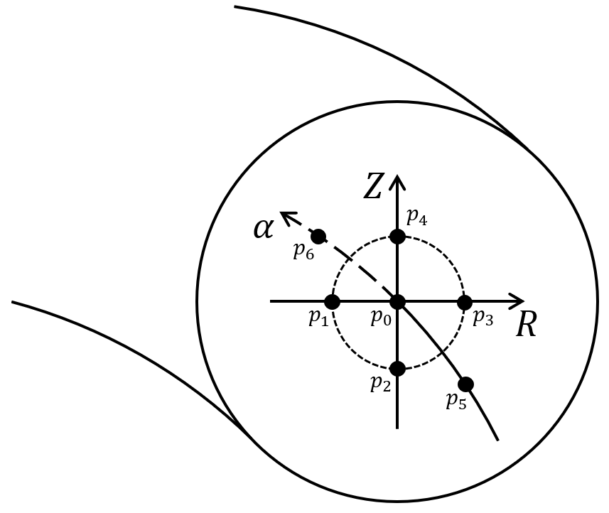
Figure 1: Partial derivative computation at the magnetic axis in field-aligned coordinates.

As is shown in Fig. (1), $p_{0}$ is a fixed grid point at the magnetic axis in field-aligned coordinates.

$$\psi|_{p_{0}} =\psi_{0},$$ (63)

$$\theta|_{p_{0}} =\theta_{j},$$ (64)

$$\alpha|_{p_{0}} =\alpha_{k}.$$ (65)

Thus, in cylindrical coordinates, partial derivatives of any scalar function $f\left(p\right)$ at $p=p_{0}$ can be numerically computed by

$$\partial_{R}f\left(p_{0}\right)=\frac{1}{R|_{p_{3}}-R|_{p_{1}}}\left(f\left(p_{3}\right)-f\left(p_{1}\right)\right),$$ (66)

$$\partial_{Z}f\left(p_{0}\right)=\frac{1}{Z|_{p_{4}}-Z|_{p_{2}}}\left(f\left(p_{4}\right)-f\left(p_{2}\right)\right),$$ (67)

$$\partial_{\zeta}f\left(p_{0}\right)=\frac{1}{\zeta|_{p_{6}}-\zeta|_{p_{5}}}\left(f\left(p_{6}\right)-f\left(p_{5}\right)\right),$$ (68)

For avoiding the high dimensional interpolation on $\psi-\theta$ plane, we take

$$\bm{X}_{f}|_{p_{1}}=\left(\psi_{1},-\pi,\zeta^{*}|_{p_{0}}\right)=\left(\psi_{1},\theta_{0},\zeta^{*}|_{p_{0}}\right),$$ (69)

$$\bm{X}_{f}|_{p_{2}}=\left(\psi_{1},-\frac{\pi}{2},\zeta^{*}|_{p_{0}}\right)=\left(\psi_{1},\theta_{\frac{1}{4}N_{\theta}},\zeta^{*}|_{p_{0}}\right),$$ (70)

$$\bm{X}_{f}|_{p_{3}}=\left(\psi_{1},0,\zeta^{*}|_{p_{0}}\right)=\left(\psi_{1},\theta_{\frac{1}{2}N_{\theta}},\zeta^{*}|_{p_{0}}\right),$$ (71)

$$\bm{X}_{f}|_{p_{4}}=\left(\psi_{1},\frac{\pi}{2},\zeta^{*}|_{p_{0}}\right)=\left(\psi_{1},\theta_{\frac{3}{4}N_{\theta}},\zeta^{*}|_{p_{0}}\right),$$ (72)

$$\bm{X}_{f}|_{p_{5}}=\left(\psi_{0},\theta|_{p_{5}},\zeta^{*}|_{p_{0}}-\Delta\zeta\right),$$ (73)

$$\bm{X}_{f}|_{p_{6}}=\left(\psi_{0},\theta|_{p_{6}},\zeta^{*}|_{p_{0}}+\Delta\zeta\right).$$ (74)

By using Eq. (61), we have

$$\zeta^{*}|_{p_{0}}=q_{0}\theta_{j}-\alpha_{k},$$ (75)

$q_{i}\equiv q\left(\psi_{i}\right)$. For convenience of computation, we choose

$$\theta|_{p_{5}} =\theta|_{p_{6}}=\theta_{j},$$ (76)

$$\Delta\zeta =\Delta\alpha,$$ (77)

then we obtain

$$\bm{X}_{l}|_{p_{1}}=\left(\psi_{1},\theta_{0},\alpha_{k}+q_{0}\left(\theta_{0}-\theta_{j}\right)\right),$$ (78)

$$\bm{X}_{l}|_{p_{2}}=\left(\psi_{1},\theta_{\frac{1}{4}N_{\theta}},\alpha_{k}+q_{0}\left(\theta_{\frac{1}{4}N_{\theta}}-\theta_{j}\right)\right),$$ (79)

$$\bm{X}_{l}|_{p_{3}}=\left(\psi_{1},\theta_{\frac{1}{2}N_{\theta}},\alpha_{k}+q_{0}\left(\theta_{\frac{1}{2}N_{\theta}}-\theta_{j}\right)\right),$$ (80)

$$\bm{X}_{l}|_{p_{4}}=\left(\psi_{1},\theta_{\frac{3}{4}N_{\theta}},\alpha_{k}+q_{0}\left(\theta_{\frac{3}{4}N_{\theta}}-\theta_{j}\right)\right),$$ (81)

$$\bm{X}_{l}|_{p_{5}}=\left(\psi_{0},\theta_{j},\alpha_{k}+\Delta_{\alpha}\right)=\begin{cases}\left(\psi_{0},\theta_{j},\alpha_{k+1}\right),&k\neq N_{\alpha}-1\\ \left(\psi_{0},\theta_{j},\alpha_{1}\right),&k=N_{\alpha}-1\end{cases}$$ (82)

$$\bm{X}_{l}|_{p_{6}}=\left(\psi_{0},\theta_{j},\alpha_{k}-\Delta_{\alpha}\right)=\begin{cases}\left(\psi_{0},\theta_{j},\alpha_{k-1}\right),&k\neq 1\\ \left(\psi_{0},\theta_{j},\alpha_{N_{\alpha}-1}\right).&k=1\end{cases}$$ (83)

By using the spatial relation of fixed grid points in field-aligned coordinates and the high-precisional 1D Fourier transform, partial derivatives in $R$, $Z$ and $\zeta$ directions of cylindrical coordinates are computed at the magnetic axis in field-aligned coordinates. Further, pull-back transform for computing the perturbed distribution function at the magnetic axis is computed by using Eqs. (51) and (54).

5 Poisson’s equation solver

In Ref. [29], Gauss’s law is used to discretized 2D Poisson’s equation in polar coordinates, thus the artificial boundary condition at the polar is not needed. We extend this algorithm from 2D polar coordinates to 3D field-aligned coordinates. In field-aligned coordinates, a scalar function is provided with the following $3$ properties.

$1$, periodic condition in $\alpha$ direction

$$f\left(\psi,\theta,\alpha\right)=\sum_{n}f_{n}\left(\psi,\theta\right)\mathrm{e}^{\mathrm{i}n\alpha}.$$ (84)

Thus, the partial differential operator in $\alpha$ direction $\partial_{\alpha}$ is converted to the algebraic operator $\mathrm{i}n$.

$2$, field-aligned periodic condition in $\theta$ direction

$$f\left(\psi,\theta\pm 2\pi,\alpha\right)=f\left(\psi,\theta,\alpha\mp 2q\left(\psi\right)\pi\right),$$ (85)

in the form of Fourier components

$$f_{n}\left(\psi_{i},\theta_{j}\pm 2\pi\right)=f_{n}\left(\psi_{i},\theta_{j}\right)\mathrm{e}^{\mp 2\mathrm{i}nq_{i}\pi},$$ (86)

which ensures that the central difference formula can be used at the boundary of $\theta$.

$3$, single valued condition at the magnetic axis. In magnetic flux coordinates, a scalar function $f_{f}\left(\bm{X}_{f}\right)$ satisfies

$$\partial_{\theta^{*}}f_{f}\biggl{|}_{\psi^{*}=0}=0.$$ (87)

In field-aligned coordinates, $f\left(\psi,\theta,\alpha\right)=f_{f}\left(\psi^{*},\theta^{*},\zeta^{*}\right)$. By using Eqs. (8)-(10), we can obtain

$$f\left(\psi_{0},\theta,\alpha\right)=f\left(\psi_{0},\theta_{0},\alpha+q_{0}\left(\theta_{0}-\theta\right)\right),$$ (88)

in the form of Fourier components

$$f_{n}\left(\psi_{0},\theta_{j}\right)=f_{n}\left(\psi_{0},\theta_{0}\right)\mathrm{e}^{\mathrm{i}nq_{0}\left(\theta_{0}-\theta_{j}\right)}.$$ (89)

The partial differential operator in $\theta$ direction $\partial_{\theta}$ are converted to the algebraic operator $-inq_{0}$.

The boundary condition in radial direction is $\phi\left(\psi_{N_{\psi}-1}\right)=0$. For each toroidal mode number $n$, by considering that $N_{\theta}-1$ equations are obtained with the single valued condition at the magnetic axis, we need another $N_{\theta}\times\left(N_{\psi}-2\right)+1$ equations to solve the perturbed field. By integrating both sides of the Eq. (2) with $\int\mathrm{d}\psi\mathrm{d}\theta J_{\bm{X}}$ and discretizing it numerically, we can obtain

$$A_{n,\mathcal{V}}\Phi_{n,\mathcal{V}}=R_{n,\mathcal{V}}\left[\rho_{n}\right]_{\mathcal{V}},$$ (90)

$$A_{n,\mathcal{V}}\equiv D_{n,\mathcal{V}}-P_{n,\mathcal{V}}+Z_{n,\mathcal{V}},$$ (91)

where $\mathcal{V}$ is the integral domain, $D_{n,\mathcal{V}}\Phi_{n,\mathcal{V}}$, $P_{n,\mathcal{V}}\Phi_{n,\mathcal{V}}$, $Z_{n,\mathcal{V}}\Phi_{n,\mathcal{V}}$ represent contributions of $\int_{\mathcal{V}_{i,j}}\mathrm{d}\psi\mathrm{d}\theta J_{\bm{X}}\nabla\cdot\left(c_{0}\nabla_{\perp}\phi_{n}\right)$, $\int_{\mathcal{V}_{i,j}}\mathrm{d}\psi\mathrm{d}\theta J_{\bm{X}}c_{1}\phi_{n}$, $\int_{\mathcal{V}_{i,j}}\mathrm{d}\psi\mathrm{d}\theta J_{\bm{X}}c_{1}\langle\phi\rangle_{FA}$, respectively; the subscript $n$ is understood in the way similar to Eq. (84). If $n\neq 0$, then $Z_{n,\mathcal{V}}=0$. In numerical, differential is discretized by using the central difference formula, the surface integral of the electric field flux is discretized by using the composite midpoint rule, the integral of the ion density is discretized by using the composite trapezoidal rule.

In the non-magnetic axis domain, $i=1,2,\cdots,N_{\psi}-2$, the integral region is $\mathcal{V}_{i,j}=\left[\psi_{i}-\frac{1}{2}\Delta_{\psi},\psi_{i}+\frac{1}{2}\Delta_{\psi}\right]\times\left[\theta_{j}-\frac{1}{2}\Delta_{\theta},\theta_{j}+\frac{1}{2}\Delta_{\theta}\right]$. We can obtain that

$$D_{n,\mathcal{V}_{i,j}}\Phi_{n,\mathcal{V}_{i,j}} =\sum_{i^{\prime}=i-1}^{i+1}\sum_{j^{\prime}=j-1}^{j+1}d_{n,\mathcal{V}_{i,j}}^{i^{\prime},j^{\prime}}\phi_{n}^{i^{\prime},j^{\prime}},$$ (92)

$$P_{n,\mathcal{V}_{i,j}}\Phi_{n,\mathcal{V}_{i,j}} =p_{n,\mathcal{V}_{i,j}}^{i,j}\phi_{n}^{i,j},$$ (93)

$$Z_{n,\mathcal{V}_{i,j}}\Phi_{n,\mathcal{V}_{i,j}} =\begin{cases}0&n\neq 0,\\ \sum_{i^{\prime}=i-1}^{i+1}\sum_{j^{\prime}=0}^{N_{\theta}-1}z_{0,\mathcal{V}_{i,j}}^{i^{\prime},j^{\prime}}\phi_{0}^{i^{\prime},j^{\prime}}&n=0,\end{cases}$$ (94)

$$R_{n,\mathcal{V}_{i,j}}\left[\rho_{n}\right]_{\mathcal{V}_{i,j}} =\sum_{i^{\prime}=i-1}^{i+1}r_{n,\mathcal{V}_{i,j}}^{i^{\prime},j}\rho_{n}^{i^{\prime},j}.$$ (95)

For example, we compute the $z_{0,\mathcal{V}_{i,j}}$ used in Eq. (94), which represents the contribution of $\int_{\mathcal{V}_{i,j}}\mathrm{d}\psi\mathrm{d}\theta J_{\bm{X}}c_{1}\langle\phi\rangle_{FA}$. If $i>1$, by using Eq. (6), we can obtain that

$$\int_{\mathcal{V}_{i,j}}\mathrm{d}\psi\mathrm{d}\theta J_{\bm{X}}c_{1}\langle\phi\rangle_{FA}= \frac{1}{8}\Delta_{\psi}\Delta_{\theta}J_{\bm{X}}^{i-1,j}c_{1}^{i-1,j}\frac{\sum_{j^{\prime}=0}^{N_{\theta}-1}J_{\bm{X}}^{i-1,j^{\prime}}\phi_{0}^{i-1,j^{\prime}}}{\sum_{j^{\prime\prime}=0}^{N_{\theta}-1}J_{\bm{X}}^{i-1,j^{\prime\prime}}}$$

$$+\frac{6}{8}\Delta_{\psi}\Delta_{\theta}J_{\bm{X}}^{i,j}c_{1}^{i,j}\frac{\sum_{j^{\prime}=0}^{N_{\theta}-1}J_{\bm{X}}^{i,j^{\prime}}\phi_{0}^{i,j^{\prime}}}{\sum_{j^{\prime\prime}=0}^{N_{\theta}-1}J_{\bm{X}}^{i,j^{\prime\prime}}}$$

$$+\frac{1}{8}\Delta_{\psi}\Delta_{\theta}J_{\bm{X}}^{i+1,j}c_{1}^{i+1,j}\frac{\sum_{j^{\prime}=0}^{N_{\theta}-1}J_{\bm{X}}^{i+1,j^{\prime}}\phi_{0}^{i+1,j^{\prime}}}{\sum_{j^{\prime\prime}=0}^{N_{\theta}-1}J_{\bm{X}}^{i+1,j^{\prime\prime}}},$$ (96)

thus,

$$z_{0,\mathcal{V}_{i,j}}^{i^{\prime},j^{\prime}}=\begin{cases}\frac{1}{8}\Delta_{\psi}\Delta_{\theta}J_{\bm{X}}^{i-1,j}c_{1}^{i-1,j}\frac{J_{\bm{X}}^{i-1,j^{\prime}}}{\sum_{j^{\prime\prime}=0}^{N_{\theta}-1}J_{\bm{X}}^{i-1,j^{\prime\prime}}}&i^{\prime}=i-1,\\ \frac{6}{8}\Delta_{\psi}\Delta_{\theta}J_{\bm{X}}^{i,j}c_{1}^{i,j}\frac{J_{\bm{X}}^{i,j^{\prime}}}{\sum_{j^{\prime\prime}=0}^{N_{\theta}-1}J_{\bm{X}}^{i,j^{\prime\prime}}}&i^{\prime}=i,\\ \frac{1}{8}\Delta_{\psi}\Delta_{\theta}J_{\bm{X}}^{i+1,j}c_{1}^{i+1,j}\frac{J_{\bm{X}}^{i+1,j^{\prime}}}{\sum_{j^{\prime\prime}=0}^{N_{\theta}-1}J_{\bm{X}}^{i+1,j^{\prime\prime}}}&i^{\prime}=i+1.\end{cases}$$ (97)

Else if $i=1$, the fomulation of the magnetic surface average at the magnetic axis need to be used. It is reduced to

$$\left\langle f\right\rangle_{FA}|_{\psi=0}=\frac{1}{4\pi^{2}}\int_{0}^{2\pi}\mathrm{d}\alpha\int_{0}^{2\pi}\mathrm{d}\theta f=f_{0}|_{\psi=0},$$ (98)

which can be used in simulation even if the space Jacobian is equal to zero. Note that $J_{\bm{X}}$ and $c_{1}$ is independent of $\theta$ at the axis, it is not difficult to obtain that

$$z_{0,\mathcal{V}_{1,j}}^{i^{\prime},j^{\prime}}=\begin{cases}\frac{1}{8}\Delta_{\psi}\Delta_{\theta}J_{\bm{X}}^{0,0}c_{1}^{0,0}&i^{\prime}=0,\\ \frac{6}{8}\Delta_{\psi}\Delta_{\theta}J_{\bm{X}}^{1,j}c_{1}^{1,j}\frac{J_{\bm{X}}^{1,j^{\prime}}}{\sum_{j^{\prime\prime}=0}^{N_{\theta}-1}J_{\bm{X}}^{1,j^{\prime\prime}}}&i^{\prime}=1,\\ \frac{1}{8}\Delta_{\psi}\Delta_{\theta}J_{\bm{X}}^{2,j}c_{1}^{2,j}\frac{J_{\bm{X}}^{2,j^{\prime}}}{\sum_{j^{\prime\prime}=0}^{N_{\theta}-1}J_{\bm{X}}^{2,j^{\prime\prime}}}&i^{\prime}=2.\end{cases}$$ (99)

It is worth pointing out that if $j=0$ or $N_{\theta}-1$, then $\phi_{n}^{i,-1}$ or $\phi_{n}^{i,N_{\theta}}$ will appear in the computation. By using the field-aligned periodic condition, we can obtain $\phi_{n}^{i,-1}=\phi_{n}^{i,N_{\theta}-1}\mathrm{e}^{2\mathrm{i}nq_{i}\pi}$ and $\phi_{n}^{i,N_{\theta}}=\phi_{n}^{i,0}\mathrm{e}^{-2\mathrm{i}nq_{i}\pi}$, and absorb $\mathrm{e}^{\pm 2\mathrm{i}nq_{i}\pi}$ into $z_{0,\mathcal{V}_{i,j}}^{i^{\prime},j^{\prime}}$. The discretized equation can always be written in the form of Eq. (90).

At the magnetic axis, $i=0$, the integral domain is $\mathcal{V}_{A}=\left[0,\frac{1}{2}\Delta_{\psi}\right]\times\left[-\pi-\frac{1}{2}\Delta_{\theta},\pi-\frac{1}{2}\Delta_{\theta}\right]$. We have

$$D_{n,\mathcal{V}_{A}}\Phi_{n,\mathcal{V}_{A}} =d_{n,\mathcal{V}_{A}}^{0,0}\phi_{n}^{0,0}+\sum_{j=0}^{N_{\theta}-1}d_{n,\mathcal{V}_{A}}^{1,j}\phi_{n}^{1,j},$$ (100)

$$P_{n,\mathcal{V}_{A}}\Phi_{n,\mathcal{V}_{A}} =p_{n,\mathcal{V}_{A}}^{0,0}\phi_{n}^{0,0}+\sum_{j^{\prime}=0}^{N_{\theta}-1}p_{n,\mathcal{V}_{A}}^{1,j^{\prime}}\phi_{0}^{1,j^{\prime}},$$ (101)

$$Z_{n,\mathcal{V}_{A}}\Phi_{n,\mathcal{V}_{A}} =\begin{cases}0&n\neq 0,\\ z_{0,\mathcal{V}_{A}}\phi_{0}^{0,0}+\sum_{j^{\prime}=0}^{N_{\theta}-1}z_{0,\mathcal{V}_{A}}^{1,j^{\prime}}\phi_{0}^{1,j^{\prime}}&n=0,\end{cases}$$ (102)

$$R_{n,\mathcal{V}_{A}}\left[\rho_{n}\right]_{\mathcal{V}_{A}} =r_{n,\mathcal{V}_{A}}^{0,0}\rho_{n}^{0,0}+\sum_{j^{\prime}=0}^{N_{\theta}-1}r_{n,\mathcal{V}_{A}}^{1,j^{\prime}}\rho_{n}^{1,j^{\prime}}.$$ (103)

For example, we compute the $d_{n,\mathcal{V}_{A}}$ used in Eq. (100), which represent the contribution of $\int_{\mathcal{V}_{i,j}}\mathrm{d}\psi\mathrm{d}\theta J_{\bm{X}}\nabla\cdot\left(c_{0}\nabla_{\perp}\phi_{n}\right)$.

$$\int_{\mathcal{V}_{A}}\mathrm{d}\psi\mathrm{d}\theta J_{s}\nabla\cdot\left(c_{0}\nabla_{\perp}\phi_{n}\right)=I_{n,\mathcal{V}_{A}}^{\psi}+I_{n,\mathcal{V}_{A}}^{\theta}+I_{n,\mathcal{V}_{A}}^{\alpha},$$ (104)

with

$$I_{n,\mathcal{V}_{A}}^{\psi}\equiv \int\mathrm{d}\psi\mathrm{d}\theta\partial_{\psi}\left(C_{\psi\psi}\partial_{\psi}\phi_{n}+C_{\psi\theta}\partial_{\theta}\phi_{n}+\mathrm{i}nC_{\psi\alpha}\phi_{n}\right)$$

$$= \int_{-\pi-\frac{1}{2}\Delta_{\theta}}^{\pi-\frac{1}{2}\Delta_{\theta}}\mathrm{d}\theta\left(C_{\psi\psi}\partial_{\psi}\phi_{n}+C_{\psi\theta}\partial_{\theta}\phi_{n}+\mathrm{i}nC_{\psi\alpha}\phi_{n}\right)|_{\psi=\frac{1}{2}\Delta_{\psi}},$$ (105)

$$I_{n,\mathcal{V}_{A}}^{\theta}\equiv \int_{\mathcal{V}_{A}}\mathrm{d}\psi\mathrm{d}\theta\partial_{\theta}\left(C_{\theta\psi}\partial_{\psi}\phi_{n}+C_{\theta\theta}\partial_{\theta}\phi_{n}+\mathrm{i}nC_{\theta\alpha}\phi_{n}\right)$$

$$= \int_{0}^{\frac{1}{2}\Delta_{\psi}}\mathrm{d}\psi\left(C_{\theta\psi}\partial_{\psi}\phi_{n}+C_{\theta\theta}\partial_{\theta}\phi_{n}+\mathrm{i}nC_{\theta\alpha}\phi_{n}\right)|_{\theta=\pi-\frac{1}{2}\Delta_{\psi}}$$

$$-\int_{0}^{\frac{1}{2}\Delta_{\psi}}\mathrm{d}\psi\left(C_{\theta\psi}\partial_{\psi}\phi_{n}+C_{\theta\theta}\partial_{\theta}\phi_{n}+\mathrm{i}nC_{\theta\alpha}\phi_{n}\right)|_{\theta=-\pi-\frac{1}{2}\Delta_{\psi}},$$ (106)

$$I_{n,\mathcal{V}_{A}}^{\alpha}\equiv \int_{\mathcal{V}_{A}}\mathrm{d}\psi\mathrm{d}\theta\mathrm{i}n\left(C_{\alpha\psi}\partial_{\psi}\phi_{n}+C_{\alpha\theta}\partial_{\theta}\phi_{n}+C_{\alpha\alpha}\mathrm{i}n\phi_{n}\right),$$ (107)

and

$$C_{X_{l}^{a}X_{l}^{b}} \left(\psi,\theta\right)=\begin{cases}J_{s}c_{0}\nabla\theta\cdot\nabla\theta-\frac{c_{0}}{J_{\bm{X}}B^{2}},&X_{l}^{a}=X_{l}^{b}=\theta\\ J_{s}c_{0}\nabla X_{l}^{a}\cdot\nabla X_{l}^{b},&other\end{cases}.$$ (108)

The natural boundary condition

$$\left(C_{\psi\psi}\partial_{\psi}\phi_{n}+C_{\psi\theta}\partial_{\theta}\phi_{n}+\mathrm{i}nC_{\psi\alpha}\phi_{n}\right)_{\psi=0}=0,$$ (109)

is always satisfied, which makes the artificial boundary condition unnecessary. If $\psi$ is chosen as the radial coordinate $x$, $\nabla x\cdot\nabla x\partial_{x}\phi=\nabla x\cdot\nabla\theta\partial_{\theta}\phi=\nabla x\cdot\nabla\alpha\partial_{\alpha}\phi=0$; If $\sqrt{\psi}$ or $r$ is chosen as $x$, $J_{x,\theta,\alpha}\partial_{x}\phi=J_{x,\theta,\alpha}\partial_{\theta}\phi=J_{x,\theta,\alpha}\partial_{\alpha}\phi=0$. It can be obtained that

$$d_{n,\mathcal{V}_{A}}^{0,0}= \left[-\frac{1}{2}C_{\psi\theta}^{1/4,N_{\theta}-1/2}-\frac{3}{8}\mathrm{i}n\Delta_{\psi}\left(q_{0}C_{\theta\theta}^{1/4,N_{\theta}-1/2}-C_{\theta\alpha}^{1/4,N_{\theta}-1/2}\right)\right]\mathrm{e}^{-\mathrm{i}nq_{0}(2\pi-\Delta_{\theta}/2)}$$ (110)

$$+\left[\frac{1}{2}C_{\psi\theta}^{1/4,-1/2}+\frac{3}{8}\mathrm{i}n\Delta_{\psi}\left(q_{0}C_{\theta\theta}^{1/4,-1/2}-C_{\theta\alpha}^{1/4,-1/2}\right)\right]\mathrm{e}^{\mathrm{i}nq_{0}\Delta_{\theta}/2}$$

$$-\sum_{j=0}^{N_{\theta}-1}\biggl{[}h_{\psi}\Delta_{\theta}C_{\psi\psi}^{1/2,j}+\frac{1}{2}\mathrm{i}n\Delta_{\theta}\left(q_{0}C_{\psi\theta}^{1/2,j}-C_{\psi\alpha}^{1/2,j}+c_{\psi\alpha}^{1/4,j}\right)$$

$$-\frac{3}{8}n^{2}\Delta_{\psi}\Delta_{\theta}\left(q_{0}C_{\theta\alpha}^{1/4,j}-C_{\alpha\alpha}^{1/4,j}\right)\biggr{]}\mathrm{e}^{\mathrm{i}nq_{0}(\theta_{0}-\theta_{j})},$$

and

$$d_{n,\mathcal{V}_{A}}^{1,j}= \begin{cases}h_{\psi}\Delta_{\theta}C_{\psi\psi}^{1/2,0}+\frac{1}{2}\mathrm{i}n\Delta_{\theta}C_{\psi\alpha}^{1/2,0}\\ +\frac{1}{4}\left(C_{\psi\theta}^{1/2,N_{\theta}-1}\mathrm{e}^{-\mathrm{i}n2q_{1}\pi}-C_{\psi\theta}^{1/2,1}\right)+\frac{1}{2}\mathrm{i}n\Delta_{\theta}C_{\psi\alpha}^{1/4,0}\\ +\frac{1}{16}\mathrm{i}n\Delta_{\psi}\left(C_{\theta\alpha}^{1/4,N_{\theta}-1}\mathrm{e}^{-\mathrm{i}n2q_{1}\pi}-C_{\theta\alpha}^{1/4,1}\right)-\frac{1}{8}n^{2}\Delta_{\psi}\Delta_{\theta}C_{\alpha\alpha}^{1/4,0}\\ +\left(\frac{1}{4}C_{\psi\theta}^{1/4,N_{\theta}-1/2}+\frac{1}{8}\Delta_{\psi}h_{\theta}C_{\theta\theta}^{1/4,N_{\theta}-1/2}+\frac{1}{16}\mathrm{i}n\Delta_{\psi}C_{\theta\alpha}^{1/4,N_{\theta}-1/2}\right)\mathrm{e}^{-\mathrm{i}n2q_{1}\pi}\\ -\left(\frac{1}{4}C_{\psi\theta}^{1/4,-1/2}+\frac{1}{8}\Delta_{\psi}h_{\theta}c_{\theta\theta}^{1/4,-1/2}+\frac{1}{16}\mathrm{i}n\Delta_{\psi}C_{\theta\alpha}^{1/4,-1/2}\right),&j=0\\ \\ h_{\psi}\Delta_{\theta}C_{\psi\psi}^{1/2,N_{\theta}-1}+\frac{1}{2}\mathrm{i}n\Delta_{\theta}C_{\psi\alpha}^{1/2,N_{\theta}-1}\\ +\frac{1}{4}\left(C_{\psi\theta}^{1/2,N_{\theta}-2}-C_{\psi\theta}^{1/2,0}\mathrm{e}^{\mathrm{i}n2q_{1}\pi}\right)+\frac{1}{2}\mathrm{i}n\Delta_{\theta}C_{\psi\alpha}^{1/4,N_{\theta}-1}\\ +\frac{1}{16}\mathrm{i}n\Delta_{\psi}\left(C_{\theta\alpha}^{1/4,N_{\theta}-2}-C_{\theta\alpha}^{1/4,0}\mathrm{e}^{\mathrm{i}n2q_{1}\pi}\right)-\frac{1}{8}n^{2}\Delta_{\psi}\Delta_{\theta}C_{\alpha\alpha}^{1/4,N_{\theta}-1}\\ +\left(\frac{1}{4}C_{\psi\theta}^{1/4,N_{\theta}-1/2}-\frac{1}{8}\Delta_{\psi}h_{\theta}C_{\theta\theta}^{1/4,N_{\theta}-1/2}+\frac{1}{16}\mathrm{i}n\Delta_{\psi}C_{\theta\alpha}^{1/4,N_{\theta}-1/2}\right)\\ -\left(\frac{1}{4}C_{\psi\theta}^{1/4,-1/2}-\frac{1}{8}\Delta_{\psi}h_{\theta}C_{\theta\theta}^{1/4,-1/2}+\frac{1}{16}\mathrm{i}n\Delta_{\psi}C_{\theta\alpha}^{1/4,-1/2}\right)\mathrm{e}^{\mathrm{i}n2q_{1}\pi},&j=N_{\theta}-1\\ \\ h_{\psi}\Delta_{\theta}C_{\psi\psi}^{1/2,j}+\frac{1}{2}\mathrm{i}n\Delta_{\theta}\left(c_{\psi\alpha}^{1/2,j}+C_{\psi\alpha}^{1/4,j}\right)+\frac{1}{4}(C_{\psi\theta}^{1/2,j-1}-C_{\psi\theta}^{1/2,j+1})\\ +\frac{1}{16}\mathrm{i}n\Delta_{\psi}\left(C_{\theta\alpha}^{1/4,j-1}-C_{\theta\alpha}^{1/4,j+1}\right)-\frac{1}{8}n^{2}\Delta_{\psi}\Delta_{\theta}C_{\alpha\alpha}^{1/4,j}.&other\end{cases}$$ (111)

where $C_{X_{l}^{a}X_{l}^{b}}^{i,j}\equiv C_{X_{l}^{a}X_{l}^{b}}\left(i\Delta_{\psi},\theta_{0}+j\Delta_{\theta}\right)$. Similarly, we can obtain elements $p_{n,\mathcal{V}_{A}}^{i,j}$, $z_{n,\mathcal{V}_{A}}^{i,j}$, $r_{n,\mathcal{V}_{A}}^{i,j}$ of matrix $P_{n,\mathcal{V}_{A}}$, $Z_{n,\mathcal{V}_{A}}$, $R_{n,\mathcal{V}_{A}}$, respectively.

Thus, $1$ equation is obtained at the magnetic axis domain. Combined with $N_{\theta}\times\left(N_{\psi}-2\right)$ equations obtained in the non-magnetic axis domain and another $N_{\theta}-1$ equations obtained by the single valued condition at the magnetic axis, we have got Eq. (90), $N_{\theta}\times\left(N_{\psi}-1\right)$ equations in total, for solving the perturbed electrostatic potential.

To reduce the computational cost, we organize the field matrix as follow

$$\begin{aligned} \Phi_{n}\end{aligned}=\left[\begin{array}[]{ccccc}\Phi_{n,0},&\cdots,&\Phi_{n,i},&\cdots,&\Phi_{n,N_{\psi}-1}\end{array}\right]^{T},$$ (113)

$$\Phi_{n,i}=\left[\phi_{n}^{i,0},\cdots,\phi_{n}^{i,j},\cdots,\phi_{n}^{i,N_{\theta}-1}\right],$$ (114)

and $\left[\rho_{n}\right]$ is also organized as $\Phi_{n}$. Thus, the coefficient matrix $\left[A_{n}\right]$ is composed of block matrix $\left[A_{n}^{i,i^{\prime}}\right]$

$$A_{n}=\left[A_{n}^{i,i^{\prime}}\right],$$ (115)

$$A_{n}^{i,i^{\prime}}=\left[a_{n,i,i^{\prime}}^{j,j^{\prime}}\right],$$ (116)

$$a_{n,i,i^{\prime}}^{j,j^{\prime}}=\begin{cases}d_{n,\mathcal{V}_{i,j}}^{i^{\prime},j^{\prime}}-p_{n,\mathcal{V}_{i,j}}^{i^{\prime},j^{\prime}}+z_{n,\mathcal{V}_{i,j}}^{i^{\prime},j^{\prime}}&i\neq 0,\\ d_{n,\mathcal{V}_{A}}^{i^{\prime},j^{\prime}}-p_{n,\mathcal{V}_{A}}^{i^{\prime},j^{\prime}}+z_{n,\mathcal{V}_{A}}^{i^{\prime},j^{\prime}}&i=0,j=0,\\ \delta_{ii^{\prime}}\mathrm{e}^{\mathrm{i}nq_{0}\left(\theta_{0}-\theta_{j}\right)}&i=0,j\neq 0,j^{\prime}=0,\\ -\delta_{ii^{\prime}}\delta_{jj^{\prime}}&i=0,j\neq 0,j^{\prime}\neq 0,\end{cases}$$ (117)

and $a_{n,i,i^{\prime}}^{j,j^{\prime}}$ represents the matrix element of $A_{n}^{i,i^{\prime}}$. We can easily find that $A_{n}^{i,i^{\prime}}=0$ if $\left|i^{\prime}-i\right|>1$, $A_{n}$ is a block tridiagonal matrix. The algebraic equations can be solved by using the tridiagonal matrix algorithm.

6 Numerical filter

On the one hand, because the inner damping buffer region is not used, the filter in the radial direction is replaced by the low-pass filter. On the other hand, an additional condition for truncating the shortwave in poloidal direction is used,

$$k_{\theta}\rho_{s}=\frac{|m|}{r}\frac{\sqrt{m_{i}T_{i}}}{e_{i}B}<\left[k_{\theta}\rho\right]_{max}.$$ (118)

Thus, we have

$$|m|<m_{max}\equiv\min\left\{r\frac{e_{i}B}{\sqrt{m_{i}T_{i}}}\left[k_{\theta}\rho\right]_{max},\frac{\tilde{N}_{\theta}}{3}\right\},$$ (119)

where $\tilde{N}_{\theta^{*}}$ represents the total number of the poloidal grid point in the $\theta^{*}$ direction. It is necessary that $N_{\theta^{*}}\ll N_{\theta}$ to describe poloidal mode structures. By considering the parallel wavelength truncated condition $-\frac{N_{\theta}}{3}<m-nq\left(\psi\right)<\frac{N_{\theta}}{3}$, we have

$$|n|<n_{max}\equiv\min\left\{\frac{1}{q}\left(m_{max}+\frac{N_{\theta}}{3}\right),\frac{N_{\alpha}}{3}\right\}.$$ (120)

Finally, the filter conditions of $m$ and $n$ are

$$n \in\left(-n_{max},n_{max}\right),$$ (121)

$$m \in\left(-m_{max},m_{max}\right)\text{$\bigcap$}\left(nq-\frac{N_{\theta}}{3},nq+\frac{N_{\theta}}{3}\right).$$ (122)

In the ITG turbulence, the typical value of $k_{\perp}\rho_{i}$ is about $0.3$, thus we take $\left[k_{\theta}\rho\right]_{max}=3$ and $\tilde{N}_{\theta}=512$.

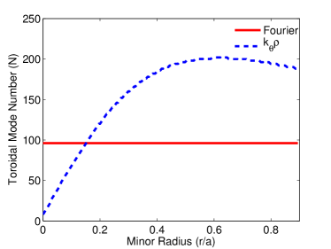
Figure 2: Relation between the truncation of the toroidal mode number and the radial positon. Red solid line: The truncated condition decided by the parallel and the poloidal wavelength, $\frac{1}{q}\left(m_{max}+\frac{N_{\theta}}{3}\right)$. Blue dash line: The truncated condition decided by the toroidal wavelength. Read solid line is the truncated condition, $\frac{N_{\alpha}}{3}$. The applied truncated condition in simulation is determined by the smaller one of above $2$ conditions.

As is shown in Fig. (2), the untruncated toroidal mode number in the ITG simulation is reduced with the radius near the magnetic axis.

7 Simulation results

In this section, nonlinear simulation results of the cyclone base test are shown. The parameters are chosen as those in Ref. [30] to compare with the results computed by GENE, ORB5. $q$ profile is

$$q\left(r\right)=0.86-0.16\frac{r}{a}+2.52\left(\frac{r}{a}\right)^{2}.$$ (123)

$q\left(r_{0}\right)=1.41$, magnetic share $\hat{s}\left(r_{0}\right)\equiv\frac{r}{q}\frac{\mathrm{d}q}{\mathrm{d}r}\left(r_{0}\right)=0.84$ with $r_{0}=0.5a$. The initial ion temperature and density profile are

$$\hat{A}\left(r\right)=\frac{A\left(r\right)}{A\left(r_{0}\right)}=\exp\left[-\kappa_{A}\frac{a}{R_{0}}\Delta_{A}\tanh\left(\frac{r-r_{0}}{a}\right)\right],$$ (124)

where $A$ can be chosen as either $T_{i}$ or $n_{i}$, and $T_{i}\left(r_{0}\right)=1.97\mathrm{keV}$, $n\left(r_{0}\right)=10^{19}\mathrm{m}^{-3}$, $\Delta_{A}=0.30$, $\kappa_{n}\equiv R_{0}/L_{n}=2.23$, $\kappa_{T_{i}}=R_{0}/L_{T_{i}}=6.96$. $L_{n}$ and $L_{T_{i}}$ represents the scale length of density and ion temperature, respectively. The pure deuterium ion and the adiabatic electron are adopted. The ratio of the ion Larmor radius and the minor radius is $\rho^{*}\equiv\rho_{s}/a=1/179$ with $\rho_{s}=c_{s}/\Omega_{i}$, $c_{s}=\sqrt{T_{i0}/m_{i}}$, $\Omega_{i}=e_{i}B_{0}/m_{i}$. The radial simulation domain including the magnetic axis is about $160\rho_{s}$, the grid resolution of this simulation is taken as $N_{\psi}\times N_{\theta}\times N_{\alpha}\times N_{V_{\parallel}}\times N_{\mu}=189\times 16\times 141\times 64\times 16$. Note that if $\psi$ is chosen as the radial coordinate, the radial resolution is coarse near the magnetic axis. The simulation with $\sqrt{\psi}$ being the radial coordinate is also computed as a comparison. In the rest of this section, NLT1, NLT2, NLT3 represent simulations by using the version of NLT without magnetic axis, with magnetic axis and $\psi$ being the radial coordinate, with magnetic axis and $\sqrt{\psi}$ being the radial coordinate, respectively.

Time evolutions of the ion heat diffusivity are shown in Fig. (3).

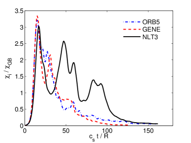
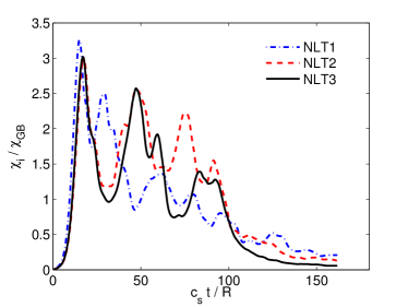
Figure 3: Time evolutions of the ion heat diffusivity $\chi_{i}/\chi_{GB}$, with $\chi_{GB}\equiv\frac{\rho_{i}^{2}c_{s}}{a}$.

It can be seen that the relaxation process obtained by using NLT with magnetic axis is step-like, which is not observed in previous simulation of relaxation process. Perturbation of the ion gyrocenter center number with time is shown in Fig. (4).

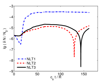
Figure 4: Time evolutions of the perturbed ion gyrocenter number, with $\delta N=\int\mathrm{d}^{6}Z\delta F$, $N_{0}=\int\mathrm{d}^{6}ZF_{0}$.

The gyrocenter conservation is much improved by including the magnetic axis in the simulation domain. The zonal field is shown in Fig. (5).

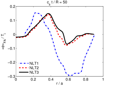
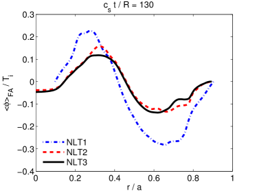
Figure 5: Zonal field $\left\langle\phi\right\rangle_{FA}$. Left and right figures show the zonal field at $\frac{c_{s}t}{R}=50$ and $\frac{c_{s}t}{R}=130$, respectively.

Zonal fields obtained in NLT2 and NLT3 are similar with each other, however, they are obviously different from the result obtained in NLT1. The zonal electrostatic potential is nonzero, and the gradient of the zonal electrostatic potential at the magnetic axis is almost zero, which is reasonable. Fig. (6) shows the contours of the non-zonal electrostatic potential.

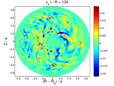
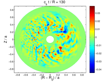
Figure 6: Contours of the non-zonal electrostatic potential $\phi-\left\langle\phi\right\rangle_{FA}$ at $\frac{c_{s}t}{R}=130$. Left and right figures are the results in NLT3 and NLT1, respectively.

The radial distribution of the perturbed electrostatic potential obtained in simulation with magnetic axis is also different from that in simulation without magnetic axis.

8 Summary and discussion

Simulation domain of the electrostatic gyrokinetic nonlinear turbulence global code, NLT, is extended to include the magnetic axis in field-aligned coordinates. In the first part of NLT for computing the unperturbed guiding center orbit, Hamilton’s equations in cylindrical coordinates are solved when the guiding center is close to the magnetic axis, thus the singularity of Poisson matrix in field-aligned coordinates are avoided. Note that the unperturbed orbit is unchanged in NLT simulation, which can be computed only once by using the high-precisional numerical algorithm in the initial. The second part of NLT is the pull-back transform, which is equivalent to compute the perturbed orbit. As the method used in the first part, the pull-back transform at the magnetic axis is computed by using formulations in cylindrical coordinates for avoiding the singularity of Poisson matrix in field-aligned coordinates. Numerically, partial derivatives in $R$ and $Z$ directions of cylindrical coordinates are computed by using values at grid points $\left(\psi=\Delta_{\psi},\theta=-\pi\right)$, $\left(\psi=\Delta_{\psi}\theta=0\right)$ and $\left(\psi=\Delta_{\psi},\theta=-\pi/2\right)$, $\left(\psi=\Delta_{\psi},\theta=\pi/2\right)$ in field-aligned coordinates and combining the toroidal Fourier transform. All these four points are grid points in the $\psi-\theta$ plane. Thus, the coordinate transform from field-aligned coordinates to cylindrical coordinates is not needed in NLT. The third part, Birdsell’s method[29] is extended from 2D polar coordinates to 3D field-aligned coordinates for solving the gyrokinetic quasi-neutrality equation in the long-wavelength approximation with adiabatic electrons. The integral format is used to discretized the equation, the boundary condition at the magnetic axis is the natural boundary condition instead of a artificial boundary condition. The zonal field is solved directly from the equation without using the magenetic surface averaged equation. The coefficient matrix of the discretized algebraic equation is a block tridiagonal matrix, the tridiagonal matrix algorithm is used to reduce the computational cost. In the fourth part, numerical filtering, a new condition for limiting the shortwave in the $\theta^{*}$ direction,$\frac{m}{r}\rho_{s}<\left[k_{\theta}\rho\right]_{max}$, is considered. At the region near the magnetic axis, the retained toroidal mode number is reduced with the radius by considering this new condition.

In the nonlinear ITG test, the gyrocenter conservation is much improved by including the magnetic axis in the simulation domain. The zonal field and the radial distribution of the perturbed electrostatic potential are different from previous results without the magnetic axis.

The numerical algorithm for treating the self-consistent simulation including the magnetic axis in field-aligned coordinates is presented in this paper. Although the algorithm is used in numerical Lie transform code, the key idea for treating the singularity and boundary condition at magnetic axis can also be used in different simulation codes. In the electromagnetic simulation, equation of Ampere’s law is also in the form same with Poisson’s equation, should be numerically discretized with integral format.

Reference