Adversarial Propagation and Zero-Shot Cross-Lingual Transfer
of Word Vector Specialization

Abstract

Semantic specialization is a process of fine-tuning pre-trained distributional word vectors using external lexical knowledge (e.g., WordNet) to accentuate a particular semantic relation in the specialized vector space. While post-processing specialization methods are applicable to arbitrary distributional vectors, they are limited to updating only the vectors of words occurring in external lexicons (i.e., seen words), leaving the vectors of all other words unchanged. We propose a novel approach to specializing the full distributional vocabulary. Our adversarial post-specialization method propagates the external lexical knowledge to the full distributional space. We exploit words seen in the resources as training examples for learning a global specialization function. This function is learned by combining a standard $L_{2}$-distance loss with a adversarial loss: the adversarial component produces more realistic output vectors. We show the effectiveness and robustness of the proposed method across three languages and on three tasks: word similarity, dialog state tracking, and lexical simplification. We report consistent improvements over distributional word vectors and vectors specialized by other state-of-the-art specialization frameworks. Finally, we also propose a cross-lingual transfer method for zero-shot specialization which successfully specializes a full target distributional space without any lexical knowledge in the target language and without any bilingual data.

1 Introduction

Word representation learning is a mainstay of modern Natural Language Processing (NLP), and its usefulness has been proven across a wide spectrum of NLP applications (Collobert et al., 2011; Chen and Manning, 2014; Melamud et al., 2016b, inter alia). Standard distributional word vector models are grounded in the distributional hypothesis Harris (1954), that is, they leverage information about word co-occurrences in large text corpora Mikolov et al. (2013); Pennington et al. (2014); Levy and Goldberg (2014); Bojanowski et al. (2017). This dependence on contextual signal results in a well-known tendency to conflate semantic similarity with other types of semantic association Hill et al. (2015); Schwartz et al. (2015); Vulić et al. (2017) in the induced word vector spaces.

A common remedy is to move beyond purely unsupervised word representation learning, in a process referred to as semantic specialization or retrofitting. Specialization methods exploit lexical knowledge from external resources, such as WordNet Fellbaum (1998) or the Paraphrase Database Ganitkevitch et al. (2013) to refine the semantic properties of pre-trained vectors and specialize the distributional spaces for a particular relation, e.g., synonymy (i.e., true similarity) Faruqui et al. (2015); Mrkšić et al. (2017) or hypernymy Nickel and Kiela (2017); Nguyen et al. (2017); Vulić and Mrkšić (2018).

The best-performing specialization models (cf. Mrkšić et al. 2017) are deployed as post-processors of the vector space: distributional vectors are fine-tuned to satisfy linguistic constraints extracted from external resources to offer improved support to downstream NLP applications Faruqui (2016). Such models are versatile as they can be applied to arbitrary distributional spaces, but they have a major drawback: they locally update only vectors of words present in linguistic constraints (i.e., seen words), whereas vectors of all other (i.e., unseen) words remain intact (see Figure 1).

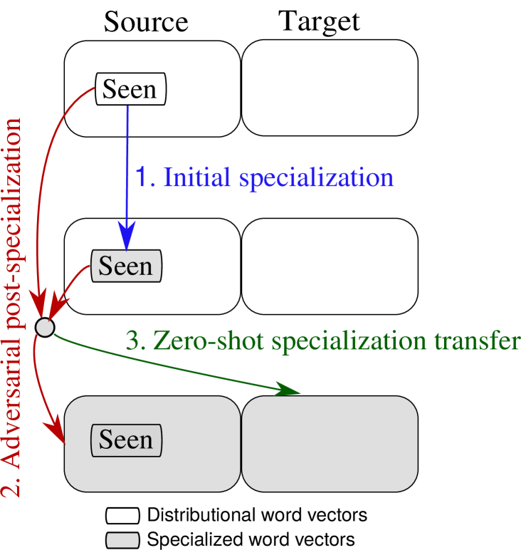
Figure 1: High-level illustration of the adversarial post-specialization process and cross-lingual zero-shot specialization, described in detail in §2.

Vulić et al. (2018) have recently proposed a model which, based on the updates of vectors of seen words, learns a global specialization function that can be applied to the large subspace of unseen words. Their global method, termed post-specialization and implemented as a deep feed-forward network, effectively specializes all distributional vectors.

In this paper, we propose a new approach to post-specialization which addresses the following two research questions: a) Is it possible to use a more sophisticated learning approach to yield more realistic specialized vectors for the full vocabulary? b) Given that specialization methods inherently require a large number of constraints, is it possible to specialize distributional word vectors where such resources are scarce or non-existent? Our novel model learns the global specialization function by casting the feed-forward specialization network as a generator component of an adversarial architecture, see Figure 2. The corresponding discriminator component learns to discern original specialized vectors (produced by any local specialization model) from vectors produced by transforming distributional vectors with the feed-forward post-specialization network (i.e., the generator).

We show that the proposed adversarial model yields state-of-the-art performance on standard word similarity benchmarks, outperforming the post-specialization model of Vulić et al. (2018). We further demonstrate the effectiveness of the proposed model in two downstream tasks: lexical text simplification and dialog state tracking. Finally, we demonstrate that, by coupling our adversarial specialization model with any unsupervised model for inducing bilingual vector spaces, such as the algorithm proposed by Conneau et al. (2018), we can successfully perform zero-shot language transfer of the specialization, that is, we can specialize distributional spaces of languages without any linguistic constraints in those languages, and without any bilingual data.

2 Methodology

The post-specialization procedure Vulić et al. (2018) is a two-step process. First, a subspace of vectors for words observed in external resources is fine-tuned using any off-the-shelf specialization model, such as the original retrofitting model Faruqui et al. (2015), counter-fitting Mrkšić et al. (2016), dLCE Nguyen et al. (2016), or state-of-the-art attract-repel (ar) specialization Mrkšić et al. (2017); Vulić et al. (2017). We outline the initial specialization algorithms in §2.1. In the second step, the initial specialization is propagated to the entire vocabulary, including words not observed in the resources, relying on an adversarial architecture augmented with a distance loss. This adversarial post-specialization model, compatible with any specialization model, is described in §2.2.

Finally, in §2.3, we introduce a cross-lingual zero-shot specialization model which transfers the specialization to a target language without any lexical resources. An overview of the proposed methodology from this section is provided in Figure 1.

2.1 Initial Specialization

Linguistic Constraints.

Adopting the nomenclature from Mrkšić et al. (2017), post-processing models are generally guided by two broad sets of constraints: 1) attract constraints specify which words should be close to each other in the fine-tuned vector space (e.g. synonyms like graceful and amiable); 2) repel constraints describe which words should be pulled away from each other (e.g. antonyms like innocent and sinful). Earlier post-processors Faruqui et al. (2015); Jauhar et al. (2015); Wieting et al. (2015) operate only with attract constraints, and are thus not suited to model both aspects contributing to the specialization process.

We first outline the state-of-the-art attract-repel specialization model Mrkšić et al. (2017) which leverages both sets of constraints. Here, we again stress two important aspects relevant to our post-specialization model: a) all initial specialization models fine-tune only representations for the subspace of words seen in the external constraints, while all other words remain unaffected by specialization; b) post-specialization is not tied to attract-repel in particular; it is applicable on top of any other post-processor.

Specialization of Seen Words.

The key idea is to inject the knowledge from linguistic constraints into pre-trained distributional word vectors. Given a set $A$ of attract word pairs and a set $R$ of repel word pairs, each word pair $(v_{l},v_{r})$ from the vocabulary $\mathcal{V}_{s}$ of seen words present in these sets can be represented as a vector pair ($\textbf{x}_{l},\textbf{x}_{r})$.

The optimization is driven by mini-batches of attract pairs $\mathcal{B}_{A}$ (batch size $k_{A}$), and of repel pairs $\mathcal{B}_{R}$ (size $k_{R}$). For both of these, two sets of negative example pairs of equal size are drawn from the $2(k_{A}+k_{R})$ vectors occurring in $\mathcal{B}_{A}$ and $\mathcal{B}_{R}$. This defines the mini-batches $T_{A}({B}_{A})=[(\mathbf{t}_{l}^{1},\mathbf{t}_{r}^{1})\dots(\mathbf{t}_{l}^{k_{A}},\mathbf{t}_{r}^{k_{A}})]$ and $T_{R}({B}_{R})=[(\mathbf{t}_{l}^{1},\mathbf{t}_{r}^{1})\dots(\mathbf{t}_{l}^{k_{R}},\mathbf{t}_{r}^{k_{R}})]$. Negative examples $\textbf{t}_{l}$ and $\textbf{t}_{r}$ for attract (or repel) pairs are the nearest (or farthest) neighbours by cosine similarity to $\textbf{x}_{l}$ and $\textbf{x}_{r}$, respectively. They ensure that the paired vectors for words in the constraints are closer to each other (or more distant for antonyms) than to their respective negative examples.

The overall objective function consists of three terms. The first term pulls attract pairs together:

$$Att(\mathcal{B}_{A},\mathcal{T}_{A})=\sum_{i=1}^{k_{A}}\Big{[}\tau\big{(}\delta_{A}+\mathbf{x}_{l}^{i}\mathbf{t}_{l}^{i}-\mathbf{x}_{l}^{i}\mathbf{x}_{r}^{i}\big{)}+\\[-0.28453pt] +\tau\big{(}\delta_{A}+\mathbf{x}_{r}^{i}\mathbf{t}_{r}^{i}-\mathbf{x}_{l}^{i}\mathbf{x}_{r}^{i}\big{)}\Big{]}$$ (1)

$\tau(z)=\text{max}(0,z)$ is the standard rectifier (Nair and Hinton, 2010). $\delta_{A}$ is the attract margin: it specifies the tolerance for the difference between the two distances (with the other pair member and with the negative example). The second term, $Rep(\mathcal{B}_{R},\mathcal{T}_{R})$, is similar but now pushes repel pairs away from each other, relying on the repel margin $\delta_{R}$:

$$Rep(\mathcal{B}_{R},\mathcal{T}_{R})=\sum_{i=1}^{k_{R}}[\tau\left(\delta_{R}-\mathbf{x}_{l}^{i}\mathbf{t}_{l}^{i}+\mathbf{x}_{l}^{i}\mathbf{x}_{r}^{i}\right)+\\ +\tau\left(\delta_{R}-\mathbf{x}_{r}^{i}\mathbf{t}_{r}^{i}+\mathbf{x}_{l}^{i}\mathbf{x}_{r}^{i}\right)]$$ (2)

The final term is tasked to preserve the quality of the original vectors through $L_{2}$-regularization:

$$Pre(\mathcal{B}_{A},\mathcal{B}_{R})=\sum_{\textbf{x}_{i}\in\mathcal{B}_{A}\cup\mathcal{B}_{R}}\lambda_{P}||\textbf{y}_{i}-\textbf{x}_{i}||_{2}$$ (3)

$\textbf{y}_{i}$ is the vector specialized from the original distributional vector $\textbf{x}_{i}$, and $\lambda_{P}$ is a regularization hyper-parameter. The optimizer finally minimizes the following objective: $\mathcal{L}_{AR}=Att(\mathcal{B}_{A},\mathcal{T}_{A})+Rep(\mathcal{B}_{R},\mathcal{T}_{R})+Pre(\mathcal{B}_{A},\mathcal{B}_{R})$.

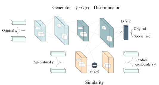
Figure 2: Architecture of the AuxGAN: an adversarial generator-discriminator loss (above) is combined with a max-margin $L_{2}$-distance loss with random confounders (below).

2.2 Adversarial Post-Specialization

Motivation.

The AR method affects only a subset of the full vocabulary $\mathcal{V}$, and consequently only a (small) subspace of the original space X (see Figure 1). In particular, it specializes the embeddings $\textbf{X}_{s}$ corresponding to $\mathcal{V}_{s}$, the vocabulary of words observed in the constraints. It leaves the embeddings $\textbf{X}_{u}$ corresponding to all other (unseen) words $\mathcal{V}_{u}$ identical.

Nevertheless, the perturbation underwent by the original observed embeddings can provide evidence about the general effects of specialization. In particular, it allows to learn a global mapping function $f:\textbf{X}\in\mathbb{R}^{d}\rightarrow\textbf{Y}\in\mathbb{R}^{d}$ for d-dimensional vectors. The parameters for this function can be trained in a supervised fashion from pairs of original and initially specialized word embeddings ($\textbf{x}_{i}^{(s)}$, $\textbf{y}_{i}^{(s)}$) from $\mathcal{V}_{s}$, as illustrated by Figure 2. Subsequently, the mapping can be applied to distributional word vectors $\textbf{x}_{u}$ from the vocabulary of unseen words $\mathcal{V}_{u}$ to predict $\textbf{\^{y}}_{u}$, their specialized counterpart. This procedure, called post-specialization, effectively propagates the information stored in the external constraints to the entire word vector space.

However, this mapping should not just model the inherent transformation, but also ensure that the resulting vector is ‘natural’. In particular, assuming that word representations lie on a manifold, the mapping should return one of its values. The intuition behind our formulation of the training objective is that: a) an $L_{2}$-distance loss can retrieve a faithful mapping whereas b) an adversarial loss can prevent unrealistic outputs, as already proven in the the visual domain Pathak et al. (2016); Ledig et al. (2017); Odena et al. (2017).

Objective Function.

The pairs of original and specialized embeddings for seen words allow to train the global mapping function. In principle, this can be any differentiable parametrized function $G(\textbf{x};\theta_{G})$. Vulić et al. (2018) showed that non-linear functions ensure a better mapping than linear transformations which seem inadequate to mimic the complex perturbations of the specialization process, guided by possibly millions of pairwise constraints. Our preliminary experiments corroborate this intuition. Thus, in this work we also opt for implementing $G(\textbf{x};\theta_{G})$ as a deep neural network. Each of the l hidden layers of size h non-linearly transforms its input. The output layer is a linear transformation into the prediction $\textbf{\^{y}}\in\mathcal{R}^{d}$.

The parameters $\theta_{G}$ are learned by minimizing the $L_{2}$ distance between the training pairs. In particular, the loss is a contrastive margin-based ranking loss with negative sampling (MM) as proposed by Weston et al. (2011, inter alia). The gist of this loss is that the first component increases the cosine similarity cos of predicted and initially specialized vectors of the same word up to a margin $\delta_{MM}$. On the other hand, the second component encourages the predicted vectors to distance themselves from $k$ random confounders. These are negative examples sampled uniformly from the batch $\mathcal{B}$ excluding the current vector:

$$\mathcal{L}_{MM}=\sum_{i=1}^{||\mathcal{V}_{s}||}\sum_{j=1|j\neq i}^{k}\tau[\delta_{MM}-\cos(G(\mathbf{x}_{i}^{(s)};\theta_{G}),\mathbf{y}_{i}^{(s)})+\\[-1.42262pt] +\cos(G(\mathbf{x}_{i}^{(s)};\theta_{G}),\mathbf{y}_{j}^{(s)})]$$ (4)

One of the original contributions of this work is combining the $L_{2}$ distance with an adversarial loss, resulting in an auxiliary-loss Generative Adversarial Network (AuxGAN) as shown in Figure 2. The role of the adversarial component, as mentioned above, is to ‘soften’ the mapping and guarantee realistic outputs from the target distribution.

The mapping can be considered a generator $G(\textbf{x}|\theta_{G})$. On top of this, a discriminator $D(\textbf{x}|\theta_{D})$, implemented also as a multi-layer neural net, tries to distinguish whether a vector is sampled from the predicted vectors or the ar-specialized vectors. Its output layer performs binary classification through softmax. The objective minimizes the loss $\mathcal{L}_{D}$:

$$\mathcal{L}_{D}=-\sum_{i=1}^{n}\log P(\text{specialized}=0|G(\mathbf{x}_{i};\theta_{G});\theta_{D})-\\[-0.28453pt] -\sum_{i=1}^{m}\log P(\text{specialized}=1|\mathbf{y}_{i};\theta_{D})$$ (5)

In a two-player game Goodfellow et al. (2014), the generator is trained to fool the discriminator by maximizing $\text{log}(1-P(0|G(\mathbf{x}_{i};\theta_{G});\theta_{D}))$. However, to avoid vanishing gradients of $G$ early on, the loss $\mathcal{L}_{G}$ is reformulated by swapping the labels of Eq. (5) as follows:

$$\mathcal{L}_{G}=-\sum_{i=1}^{n}\log P(\text{specialized}=1|G(\mathbf{x}_{i};\theta_{G});\theta_{D})-\\[-0.28453pt] -\sum_{i=1}^{m}\log P(\text{specialized}=0|\mathbf{y}_{i};\theta_{D})$$ (6)

During the optimization procedure through stochastic gradient descent, we alternate among s steps for $\mathcal{L}_{D}$, one step for $\mathcal{L}_{G}$, and one step for $\mathcal{L}_{\mathit{MM}}$ to avoid the overfitting of $D$. The reason why $s\geq 1$ is that $D$ can be kept close to a minimum of its loss function by updating $G$ less frequently.

2.3 Zero-shot Transfer to Other Languages

Once the AuxGAN has learned a global mapping function $G(\textbf{x};\theta_{G})$ in a resource-rich language, it can be directly applied to unseen words. In this work, we propose a method to additionally post-specialize the whole vocabulary $\mathcal{V}_{t}$ of a resource-poor target language. We assume a real-world scenario where no target language constraints are available to specialize it directly.

What is more, we assume that no bilingual data or dictionaries are available either. Hence, we rely on unsupervised cross-lingual word embedding induction, and in particular on Conneau et al. (2018)’s method. By virtue of these assumptions, there is no limitation to the range of potential target languages that can be specialized. Incidentally, please note that the proposed transfer method is equally applicable on top of other cross-lingual word embedding induction methods. These may require more bilingual supervision to learn the cross-lingual vector space.

After learning the shared cross-lingual word embedding space in an unsupervised fashion Conneau et al. (2018), the global post-specialization function learnt on the seen source language vectors is applied to the target language vectors, since they lie in the same shared space (see Figure 1 again). By virtue of the transfer, linguistic constraints in the source language can enhance the distributional vectors of target language vocabularies.

Conneau et al. (2018) learn a shared cross-lingual vector space as follows. They first learn a coarse initial mapping between two monolingual embedding spaces in two different languages through a GAN where the generator is a linear transformation with an orthogonal matrix Ŵ. Its loss is identical to Eq. (5) and Eq. (6), but unlike our AuxGAN model it discriminates between embeddings drawn from the source language and the target language distributions. Using the shared space, they extract for each source vector the closest target vector according to a distance metric designed to mitigate the hubness problem Radovanović et al. (2010), the Cross-Domain Similarity Local Scaling (CSLS).

This creates a bilingual synthetic dictionary that allows to further refine the coarse initial mapping. In particular, the optimal parameters for the linear mapping minimizing the $L_{2}$-distance between source-target pairs are provided by the closed-form Procrustes solution (Schönemann, 1966) based on singular value decomposition (SVD):

$$\textbf{\^{W}}=\text{arg min}_{W}||\textbf{W}\,\mathbf{X}_{t}-\mathbf{X}_{s}||_{F}=\textbf{UV}^{\top}\\ \mathbf{U\Sigma V}^{\top}=\text{SVD}(\mathbf{X}_{t}\mathbf{X}_{s}^{\top})$$ (7)

where $||\cdot||_{F}$ is the Frobenius norm. After mapping the original target embeddings into the shared space with this method, we post-specialize them with the function outlined in §2.2, learnt on the source language. This yields the specialized target vectors $\textbf{\^{Y}}_{t}=G(\textbf{\^{W}}\,\mathbf{X}_{t};\theta_{G})$.

3 Experimental Setup

Distributional Vectors.

We estimate the robustness of adversarial post-specialization by experimenting with three widely used collections of distributional English vectors. 1) sgns-w2 vectors are trained on the cleaned and tokenized Polyglot Wikipedia Al-Rfou et al. (2013) using Skip-Gram with Negative Sampling (SGNS) Mikolov et al. (2013) by Levy and Goldberg (2014) with bag-of-words contexts (window size is 2). 2) glove-cc are GloVe vectors trained on the Common Crawl Pennington et al. (2014). 3) fasttext are vectors trained on Wikipedia with a SGNS variant that builds word vectors by summing the vectors of their constituent character n-grams Bojanowski et al. (2017). All vectors are $300$-dimensional.

Constraints and Initial Specialization.

We experiment with the sets of linguistic constraints used in prior work Zhang et al. (2014); Ono et al. (2015); Vulić et al. (2018). These constraints, extracted from WordNet Fellbaum (1998) and Roget’s Thesaurus Kipfer (2009), comprise a total of 1,023,082 synonymy/attract word pairs and 380,873 antonymy/repel pairs.

Note that the sets of constraints cover only a fraction of the full distributional vocabulary, providing direct motivation for post-specialization methods which are able to specialize the full vocabulary. For instance, only 15.3% of the sgns-w2 vocabulary words are seen words present in the constraints.

The constraints are initially injected into the distributional vector space (see Figure 1 again) using attract-repel, a state-of-the-art specialization model, for which we adopt the original suggested model setup Mrkšić et al. (2017). Hyper-parameter values are set to: $\delta_{A}=0.6$, $\delta_{R}=0.0$, $\lambda_{P}=10^{-9}$. The models are trained for 5 epochs with Adagrad Duchi et al. (2011), with batch sizes set to $k_{A}=k_{R}=50$, again as in the original work.

AuxGAN Setup and Hyper-Parameters.

Both the generator and the discriminator are feed-forward nets with $l=2$ hidden layers, each of size $h=2048$, and LeakyReLU as non-linear activation Maas et al. (2013). The dropout for the input and hidden layers of the generator is 0.2 and for the input layer of the discriminator 0.1. In evaluation, the noise is blanketed out in order to ensure a deterministic mapping (Isola et al., 2017). Moreover, we smooth the golden labels for prediction by a factor of 0.1 to make the model less vulnerable to adversarial examples (Szegedy et al., 2016).

We train our model with SGD for 10 epochs of 1 million iterations each, feeding mini-batches of size 32. For each pair in a batch we generate 25 negative examples; $s=5$ (see §2.2). As a way to normalize the mini-batches (Salimans et al., 2016), these are constructed to contain exclusively either original or specialized vectors. At each epoch, the initial learning rate of 0.1 is decayed by a factor of 0.98, or 0.5 if the score on the validation set (computed as the average cosine similarity between the predicted and ar-specialized embeddings) has not increased. The hyper-parameters $k$ and $\delta_{MM}$ are tuned via grid search on the validation set.

Zero-Shot Specialization Setup.

The GAN discriminator for learning a shared cross-lingual vector space (see §2.3) has hyper-parameters identical to the AuxGAN. The generator instead is a linear layer initialized as an identity matrix and enforced to lie on the manifold of orthogonal matrices during training (Cisse et al., 2017). No dropout is used. The unsupervised validation metric for early stopping is the cosine distance between dictionary pairs extracted with the CSLS similarity metric.

4 Results and Discussion

4.1 Word Similarity

Evaluation Setup.

We first evaluate adversarial post-specialization intrinsically, using two standard word similarity benchmarks for English: SimLex-999 Hill et al. (2015) and SimVerb-3500 Gerz et al. (2016), a dataset containing human similarity ratings for 3,500 verb pairs. The evaluation measure is Spearman’s $\rho$ rank correlation between gold and predicted word pair similarity scores.

We evaluate word vectors in two settings, similar to Vulić et al. (2018). a) In the synthetic disjoint setting, we discard all linguistic constraints that contain any of the words found in SimLex or SimVerb. This means that all test words from SimLex and SimVerb are effectively unseen words, and through this setting we are able to in vitro evaluate the model’s ability to generalize the specialization function to unseen words. b) In the full setting we leverage all constraints. This is a standard “real-life” scenario where some test words do occur in the constraints, while the mapping is learned for the remaining words. We use the full setting in all subsequent downstream applications (§4.2).

	Setting: disjoint						Setting: full
	glove-cc		fasttext		sgns-w2		glove-cc		fasttext		sgns-w2
	SL	SV	SL	SV	SL	SV	SL	SV	SL	SV	SL	SV
Distributional ($\mathbf{X}$)	.407	.280	.383	.247	.414	.272	.407	.280	.383	.247	.414	.272
Specialized: Attract-Repel	.407	.280	.383	.247	.414	.272	.781	.761	.764	.744	.778	.761
Post-Specialized: post-dffn	.645	.531	.503	.340	.553	.430	.785	.764	.768	.745	.781	.763
Post-Specialized: auxgan	.652	.552	.513	.394	.581	.434	.789	.764	.766	.741	.782	.762

Table 1: Spearman’s $\rho$ correlation scores for three standard English distributional vectors spaces on English SimLex-999 (SL) and SimVerb-3500 (SV). post-dffn Vulić et al. (2018) uses a deep non-linear feed-forward network to learn the mapping function $f$. auxgan is our adversarial model (see §2.2).

We compare our model to Attract-Repel (ar), which specializes only the vectors of words occurring in the constraints. We also provide comparisons to a post-specialization model of Vulić et al. (2018) which specializes the full vocabulary, but substitutes the AuxGAN architecture from §2.2 with a deep $5$-layer feed-forward neural net also based on the max-margin loss (see Eq. (4)) to learn the mapping function (post-dffn).

Results and Analysis.

The results are summarized in Table 1. The scores suggest that the proposed adversarial post-specialization model is universally useful and robust: we observe gains over input distributional word vectors for all three vector collections. The results in the disjoint setting illustrate the core limitation of the initial specialization/post-processing models and indicate the extent of improvement achieved when generalizing the specialization function to unseen words through adversarial post-specialization. Moreover, the scores suggest that the more sophisticated adversarial post-specialization method (auxgan) outperforms post-dffn across a large number of experimental runs, verifying its effectiveness.

We observe only modest and inconsistent gains over attract-repel and post-dffn in the full setting. However, the explanation of this finding is straightforward: 99.2% of SimLex words and 99.9% of SimVerb words are present in the external constraints, making this an unrealistic evaluation scenario. The usefulness of the initial attract-repel specialization is less pronounced in real-life downstream applications in which such high coverage cannot be guaranteed, as shown in §4.2.

4.2 Downstream Tasks

We next evaluate the embedding spaces specialized with the AuxGAN method in two tasks in which discerning semantic similarity from semantic relatedness is crucial: lexical text simplification (LS) and dialog state tracking (DST).

4.2.1 Lexical Text Simplification

The goal of lexical simplification is to replace complex words (typically words that are used less often in language and are therefore less familiar to readers) with their simpler synonyms, without infringing the grammaticality and changing the meaning of the text. Replacing complex words with related words instead of true synonyms affects the original meaning (e.g., Ferrari pilot Vettel vs Ferrari airplane Vettel) and often yields ungrammatical text (e.g., they drink all pizzas).

LS Using Word Vectors.

We use Light-LS, a publicly available LS tool based on word embeddings Glavaš and Štajner (2015). Light-LS generates and then ranks substitution candidates based on similarity in the input word vector space. The quality of the space thus directly affects LS performance: by plugging any word vector space into Light-LS, we extrinsically evaluate that embedding space for LS. Furthermore, the better the embedding space captures true semantic similarity, the better the substitutions made by Light-LS.

Evaluation Setup.

We use the standard LS dataset of Horn et al. (2014). It contains 500 sentences with indicated complex words (one word per sentence) that have to be substituted with simpler synonyms. For each word, simplifications were crowdsourced from 50 human annotators. Following prior work Horn et al. (2014); Glavaš and Štajner (2015), we evaluate the performance of Light-LS using the metric that quantifies both the quality and the frequency of word replacements: Accurracy (Acc) metric is the number of correct simplifications made divided by the total number of complex words.

	glove-cc	fasttext	sgns-w2
Vector space	Acc	Acc	Acc
Distributional	.660	.578	.560
Specialized: ar	.676	.698	.644
Post-Specialized:
post-dffn	.723	.723	.709
auxgan	.717	.739	.721

Table 2: Lexical simplification results for three (post-specialized) distributional spaces.

Results and Analysis.

Scores for all three pre-trained vector spaces are shown in Table 2. Similar to the word similarity task, embedding spaces produced with post-specialization models outperform the vectors produced with ar and original distributional vectors. The gains are now more pronounced in the real-life full setup, as only 59.6 % of all indicated complex words and substitution candidates from the LS dataset are covered in the external constraints. Adversarial post-specialization (auxgan) has a slight edge over the post-specialization with a simple feed-forward network (post-dffn) for fasttext and sgns-w2 embeddings, but not for glove-cc vectors. In general, the fact that both post-specialization methods outperform attract-repel by a wide margin shows the importance of specializing the full word vector space for downstream NLP applications.

4.2.2 Dialog State Tracking

Finally, we evaluate the importance of full-vocabulary (adversarial) post-specialization in another language understanding task: dialog state tracking (DST) Henderson et al. (2014); Williams et al. (2016), which is a standard task to measure the impact of specialization in prior work Mrkšić et al. (2017). A DST model is typically the first component of a dialog system pipeline Young (2010), tasked with capturing user’s goals and updating the dialog belief state at each dialog turn. Distinguishing similarity from relatedness is crucial for DST (e.g., a dialog system should not recommend an “expensive restaurant in the west” when asked for an “affordable pub in the north”).

Evaluation Setup.

To evaluate the effects of specialized word vectors on DST, following prior work we utilize the Neural Belief Tracker (NBT), a statistical DST model that makes inferences purely based on pre-trained word vectors Mrkšić et al. (2017). Again, as in prior work the DST evaluation is based on the Wizard-of-Oz (WOZ) v2.0 dataset Wen et al. (2017); Mrkšić et al. (2017), comprising 1,200 dialogues split into training (600 dialogues), development (200), and test data (400). We report the standard DST metric: joint goal accuracy (JGA), the proportion of dialog turns where all the user’s search goal constraints were correctly identified, computed as average over 5 NBT runs.

glove-cc word vectors	JGA
Distributional	.797
Specialized: attract-repel	.817
Post-Specialized: post-dffn	.829
Post-Specialized: auxgan	.836

Table 3: English DST performance (joint goal accuracy). GloVe-CC word vectors.

Results and Analysis.

We show English DST performance in the full setting in Table 3. Only NBT performance with glove-cc vectors is reported for brevity, as similar performance gains are observed with the other two pre-trained vector collections. The results confirm our findings established in the other two tasks: a) initial ar specialization of distributional vectors is useful, but b) it is crucial to specialize the full vocabulary for improved performance (e.g., 57% of all WOZ words are present in the constraints), and c) the more sophisticated auxgan model yields additional gains.

	Similarity ($\rho$)		LS (Acc)		DST (JGA)
Vector space	IT	DE	IT	DE	IT	DE
Distrib.	.297	.417	.308	-	.681	.621
auxgan	.431	.525	.392	-	.714	.651

Table 4: Results of zero-shot specialization applied to IT and DE fasttext distributional vectors.

4.3 Cross-Lingual Zero-Shot Specialization

Evaluation Setup.

Large collections of linguistic constraints do not exist for many languages. Therefore, we test if the specialization knowledge from a resoure-rich language (i.e., English) can be transferred to resource-lean target languages (see §2.3). We simulate resource-lean scenarios using two target languages: Italian (IT) and German (DE). We evaluate zero-specialized IT and DE fasttext vectors, using English fasttext vectors as the source, on the same three tasks as before. We report the same evaluation measures, using the following evaluation data: 1) IT and DE SimLex-999 datasets Leviant and Reichart (2015) for word similarity; 2) IT lexical simplification data (SIMPITIKI) Tonelli et al. (2016); 3) IT and DE WOZ data Mrkšić et al. (2017) for DST.

Results and Analysis.

The results are summarized in Table 4. The gains over the original distributional vectors are substantial across all three tasks and for both languages. This finding indicates that the semantic content of distributional vectors can be enriched even for languages without any readily available lexical resources.

The gap between performances of language transfer and the monolingual setting is explained by the noise introduced by the bilingual vector alignment and the different ways concepts are lexicalized across languages, as studied by semantic typology (Ponti et al., 2018). Nonetheless, in the long run, these transfer results hold promise to support the specialization of vector spaces even for resource-lean languages, and their applications.

5 Related Work

Vector Space Specialization. Specialization methods embed external information into vector spaces. Some of them integrate external linguistic constraints into distributional training and jointly optimize distributional and non-distributional objectives: they modify the prior or the regularization Yu and Dredze (2014); Xu et al. (2014); Bian et al. (2014); Kiela et al. (2015), or use a variant of the SGNS-style objective Liu et al. (2015); Ono et al. (2015); Osborne et al. (2016).

Other models inject external knowledge from available lexical resources (e.g., WordNet, PPDB) into pre-trained word vectors as a post-processing step Faruqui et al. (2015); Rothe and Schütze (2015); Wieting et al. (2015); Nguyen et al. (2016); Mrkšić et al. (2016); Cotterell et al. (2016); Mrkšić et al. (2017). They offer a portable, flexible, and light-weight approach to incorporating external knowledge into arbitrary vector spaces, outperforming less versatile joint models and yielding state-of-the-art results on language understanding tasks Mrkšić et al. (2016); Kim et al. (2016); Vulić et al. (2017). By design, these methods fine-tune only vectors of words seen in external resources.

Vulić et al. (2018) suggest that specializing the full vocabulary is beneficial for downstream applications. Comparing to their work, we show that a more sophisticated adversarial post-specialization can yield further gains across different tasks and boost full-vocabulary specialization in resource-lean settings through cross-lingual transfer.

Generative Adversarial Networks. GANs were originally devised to generate images from input noise variables (Goodfellow et al., 2014). The generation process is typically conditioned on discrete labels or data from other modalities, such as text (Mirza and Osindero, 2014). Otherwise, the condition can take the form of real data in input rather than (or in addition to) noise: in this case, the generator parameters are better conceived as a mapping function. For instance, it can bridge between pixel-to-pixel (Isola et al., 2017) or character-to-pixel (Reed et al., 2016) transformations.

The GAN objective can be mixed with more traditional loss functions: in these cases, apart from trying to fool the discriminator, the generator also minimizes the distance between input and target data Pathak et al. (2016); Li and Wand (2016); Ledig et al. (2017). The distance can be formulated as the mean squared error between the input and the target (Pathak et al., 2016), their feature maps (Li and Wand, 2016), both (Zhu et al., 2016), or a loss calculated on feature maps of a deep convolutional network (Ledig et al., 2017).

In the textual domain, adversarial models have been proven to support domain adaptation (Ganin et al., 2016) and language transfer (Chen et al., 2016) by learning domain/language-invariant latent features. Adversarial training also powers unsupervised mapping between monolingual vector spaces to learn cross-lingual word embeddings Zhang et al. (2017); Conneau et al. (2018). In this work, we show how to apply adversarial techniques to the problem of vector specialization, which has a substantial impact on language understanding tasks.

6 Conclusion and Future Work

References

- Al-Rfou et al. (2013) Rami Al-Rfou, Bryan Perozzi, and Steven Skiena. 2013. Polyglot: Distributed word representations for multilingual NLP. In Proceedings of CoNLL, pages 183–192.
- Bansal et al. (2014) Mohit Bansal, Kevin Gimpel, and Karen Livescu. 2014. Tailoring continuous word representations for dependency parsing. In Proceedings of ACL, pages 809–815.
- Bian et al. (2014) Jiang Bian, Bin Gao, and Tie-Yan Liu. 2014. Knowledge-powered deep learning for word embedding. In Proceedings of ECML-PKDD, pages 132–148.
- Bojanowski et al. (2017) Piotr Bojanowski, Edouard Grave, Armand Joulin, and Tomas Mikolov. 2017. Enriching word vectors with subword information. Transactions of the ACL, 5:135–146.
- Bruni et al. (2014) Elia Bruni, Nam-Khanh Tran, and Marco Baroni. 2014. Multimodal distributional semantics. Journal of Artificial Intelligence Research, 49:1–47.
- Chen and Manning (2014) Danqi Chen and Christopher D. Manning. 2014. A fast and accurate dependency parser using neural networks. In Proceedings of EMNLP, pages 740–750.
- Chen et al. (2016) Xilun Chen, Yu Sun, Ben Athiwaratkun, Claire Cardie, and Kilian Weinberger. 2016. Adversarial deep averaging networks for cross-lingual sentiment classification. arXiv preprint arXiv:1606.01614.
- Cisse et al. (2017) Moustapha Cisse, Piotr Bojanowski, Edouard Grave, Yann Dauphin, and Nicolas Usunier. 2017. Parseval networks: Improving robustness to adversarial examples. In Proceedings of ICML, pages 854–863.
- Collobert et al. (2011) Ronan Collobert, Jason Weston, Léon Bottou, Michael Karlen, Koray Kavukcuoglu, and Pavel P. Kuksa. 2011. Natural language processing (almost) from scratch. Journal of Machine Learning Research, 12:2493–2537.
- Conneau et al. (2018) Alexis Conneau, Guillaume Lample, Marc’Aurelio Ranzato, Ludovic Denoyer, and Hervé Jégou. 2018. Word translation without parallel data. In Proceedings of ICLR (Conference Track).
- Cotterell et al. (2016) Ryan Cotterell, Hinrich Schütze, and Jason Eisner. 2016. Morphological smoothing and extrapolation of word embeddings. In Proceedings of ACL, pages 1651–1660.
- Duchi et al. (2011) John C. Duchi, Elad Hazan, and Yoram Singer. 2011. Adaptive subgradient methods for online learning and stochastic optimization. Journal of Machine Learning Research, 12:2121–2159.
- Faruqui (2016) Manaal Faruqui. 2016. Diverse Context for Learning Word Representations. Ph.D. thesis, Carnegie Mellon University.
- Faruqui et al. (2015) Manaal Faruqui, Jesse Dodge, Sujay Kumar Jauhar, Chris Dyer, Eduard Hovy, and Noah A. Smith. 2015. Retrofitting word vectors to semantic lexicons. In Proceedings of NAACL-HLT, pages 1606–1615.
- Fellbaum (1998) Christiane Fellbaum. 1998. WordNet.
- Finkelstein et al. (2002) Lev Finkelstein, Evgeniy Gabrilovich, Yossi Matias, Ehud Rivlin, Zach Solan, Gadi Wolfman, and Eytan Ruppin. 2002. Placing search in context: The concept revisited. ACM Transactions on Information Systems, 20(1):116–131.
- Ganin et al. (2016) Yaroslav Ganin, Evgeniya Ustinova, Hana Ajakan, Pascal Germain, Hugo Larochelle, François Laviolette, Mario Marchand, and Victor Lempitsky. 2016. Domain-adversarial training of neural networks. Journal of Machine Learning Research, 17(1):59:1–59:35.
- Ganitkevitch et al. (2013) Juri Ganitkevitch, Benjamin Van Durme, and Chris Callison-Burch. 2013. PPDB: The Paraphrase Database. In Proceedings of NAACL-HLT, pages 758–764.
- Gerz et al. (2016) Daniela Gerz, Ivan Vulić, Felix Hill, Roi Reichart, and Anna Korhonen. 2016. SimVerb-3500: A large-scale evaluation set of verb similarity. In Proceedings of EMNLP, pages 2173–2182.
- Glavaš and Štajner (2015) Goran Glavaš and Sanja Štajner. 2015. Simplifying lexical simplification: Do we need simplified corpora? In Proceedings of ACL, pages 63–68.
- Goodfellow et al. (2014) Ian Goodfellow, Jean Pouget-Abadie, Mehdi Mirza, Bing Xu, David Warde-Farley, Sherjil Ozair, Aaron Courville, and Yoshua Bengio. 2014. Generative adversarial nets. In Proceedings of NIPS, pages 2672–2680.
- Harris (1954) Zellig S. Harris. 1954. Distributional structure. Word, 10(23):146–162.
- Henderson et al. (2014) Matthew Henderson, Blaise Thomson, and Jason D. Wiliams. 2014. The Second Dialog State Tracking Challenge. In Proceedings of SIGDIAL, pages 263–272.
- Hill et al. (2015) Felix Hill, Roi Reichart, and Anna Korhonen. 2015. SimLex-999: Evaluating semantic models with (genuine) similarity estimation. Computational Linguistics, 41(4):665–695.
- Horn et al. (2014) Colby Horn, Cathryn Manduca, and David Kauchak. 2014. Learning a lexical simplifier using Wikipedia. In Proceedings of ACL, pages 458–463.
- Isola et al. (2017) Phillip Isola, Jun-Yan Zhu, Tinghui Zhou, and Alexei A Efros. 2017. Image-to-image translation with conditional adversarial networks. In Proceedings of CVPR, pages 1125–1134.
- Jauhar et al. (2015) Sujay Kumar Jauhar, Chris Dyer, and Eduard H. Hovy. 2015. Ontologically grounded multi-sense representation learning for semantic vector space models. In Proceedings of NAACL, pages 683–693.
- Kiela et al. (2015) Douwe Kiela, Felix Hill, and Stephen Clark. 2015. Specializing word embeddings for similarity or relatedness. In Proceedings of EMNLP, pages 2044–2048.
- Kim et al. (2016) Joo-Kyung Kim, Gokhan Tur, Asli Celikyilmaz, Bin Cao, and Ye-Yi Wang. 2016. Intent detection using semantically enriched word embeddings. In Proceedings of SLT.
- Kipfer (2009) Barbara Ann Kipfer. 2009. Roget’s 21st Century Thesaurus (3rd Edition). Philip Lief Group.
- Ledig et al. (2017) Christian Ledig, Lucas Theis, Ferenc Huszar, Jose Caballero, Andrew Cunningham, Alejandro Acosta, Andrew Aitken, Alykhan Tejani, Johannes Totz, Zehan Wang, et al. 2017. Photo-realistic single image super-resolution using a generative adversarial network. In Proceedings of CVPR, pages 4681–4690.
- Leviant and Reichart (2015) Ira Leviant and Roi Reichart. 2015. Separated by an un-common language: Towards judgment language informed vector space modeling. CoRR, abs/1508.00106.
- Levy and Goldberg (2014) Omer Levy and Yoav Goldberg. 2014. Dependency-based word embeddings. In Proceedings of ACL, pages 302–308.
- Li and Wand (2016) Chuan Li and Michael Wand. 2016. Precomputed real-time texture synthesis with markovian generative adversarial networks. In Proceedings of ECCV, pages 702–716.
- Liu et al. (2015) Quan Liu, Hui Jiang, Si Wei, Zhen-Hua Ling, and Yu Hu. 2015. Learning semantic word embeddings based on ordinal knowledge constraints. In Proceedings of ACL, pages 1501–1511.
- Maas et al. (2013) Andrew L. Maas, Awni Y. Hannun, and Andrew Y. Ng. 2013. Rectifier nonlinearities improve neural network acoustic models. In Proceedings of ICML.
- Melamud et al. (2016a) Oren Melamud, Jacob Goldberger, and Ido Dagan. 2016a. Context2vec: Learning generic context embedding with bidirectional LSTM. In Proceedings of CoNLL, pages 51–61.
- Melamud et al. (2016b) Oren Melamud, David McClosky, Siddharth Patwardhan, and Mohit Bansal. 2016b. The role of context types and dimensionality in learning word embeddings. In Proceedings of NAACL-HLT, pages 1030–1040.
- Mikolov et al. (2013) Tomas Mikolov, Ilya Sutskever, Kai Chen, Gregory S. Corrado, and Jeffrey Dean. 2013. Distributed representations of words and phrases and their compositionality. In Proceedings of NIPS, pages 3111–3119.
- Mirza and Osindero (2014) Mehdi Mirza and Simon Osindero. 2014. Conditional generative adversarial nets. arXiv preprint arXiv:1411.1784.
- Mrkšić et al. (2017) Nikola Mrkšić, Diarmuid Ó Séaghdha, Tsung-Hsien Wen, Blaise Thomson, and Steve Young. 2017. Neural belief tracker: Data-driven dialogue state tracking. In Proceedings of ACL, pages 1777–1788.
- Mrkšić et al. (2016) Nikola Mrkšić, Diarmuid Ó Séaghdha, Blaise Thomson, Milica Gašić, Lina Maria Rojas-Barahona, Pei-Hao Su, David Vandyke, Tsung-Hsien Wen, and Steve Young. 2016. Counter-fitting word vectors to linguistic constraints. In Proceedings of NAACL-HLT, pages 142–148.
- Mrkšić et al. (2017) Nikola Mrkšić, Ivan Vulić, Diarmuid Ó Séaghdha, Ira Leviant, Roi Reichart, Milica Gašić, Anna Korhonen, and Steve Young. 2017. Semantic specialisation of distributional word vector spaces using monolingual and cross-lingual constraints. Transactions of the ACL, 5:309–324.
- Nair and Hinton (2010) Vinod Nair and Geoffrey E. Hinton. 2010. Rectified linear units improve restricted Boltzmann machines. In Proceedings of ICML, pages 807–814.
- Nguyen et al. (2017) Kim Anh Nguyen, Maximilian Köper, Sabine Schulte im Walde, and Ngoc Thang Vu. 2017. Hierarchical embeddings for hypernymy detection and directionality. In Proceedings of EMNLP, pages 233–243.
- Nguyen et al. (2016) Kim Anh Nguyen, Sabine Schulte im Walde, and Ngoc Thang Vu. 2016. Integrating distributional lexical contrast into word embeddings for antonym-synonym distinction. In Proceedings of ACL, pages 454–459.
- Nickel and Kiela (2017) Maximilian Nickel and Douwe Kiela. 2017. Poincaré embeddings for learning hierarchical representations. In Proceedings of NIPS, pages 6341–6350.
- Odena et al. (2017) Augustus Odena, Christopher Olah, and Jonathon Shlens. 2017. Conditional image synthesis with auxiliary classifier gans. In Proceedings of ICML, pages 2642–2651.
- Ono et al. (2015) Masataka Ono, Makoto Miwa, and Yutaka Sasaki. 2015. Word embedding-based antonym detection using thesauri and distributional information. In Proceedings of NAACL-HLT, pages 984–989.
- Osborne et al. (2016) Dominique Osborne, Shashi Narayan, and Shay Cohen. 2016. Encoding prior knowledge with eigenword embeddings. Transactions of the ACL, 4:417–430.
- Pathak et al. (2016) Deepak Pathak, Philipp Krähenbühl, Jeff Donahue, Trevor Darrell, and Alexei A. Efros. 2016. Context encoders: Feature learning by inpainting. In Proceedings of CVPR, pages 2536–2544.
- Pennington et al. (2014) Jeffrey Pennington, Richard Socher, and Christopher Manning. 2014. Glove: Global vectors for word representation. In Proceedings of EMNLP, pages 1532–1543.
- Ponti et al. (2018) Edoardo Maria Ponti, Helen O’Horan, Yevgeni Berzak, Ivan Vulić, Roi Reichart, Thierry Poibeau, Ekaterina Shutova, and Anna Korhonen. 2018. Modeling language variation and universals: A survey on typological linguistics for natural language processing. arXiv preprint arXiv:1807.00914.
- Radovanović et al. (2010) Milos Radovanović, Alexandros Nanopoulos, and Mirjana Ivanović. 2010. Hubs in space: Popular nearest neighbors in high-dimensional data. Journal of Machine Learning Research, 11:2487–2531.
- Reed et al. (2016) Scott Reed, Zeynep Akata, Xinchen Yan, Lajanugen Logeswaran, Bernt Schiele, and Honglak Lee. 2016. Generative adversarial text to image synthesis. In Proceedings of ICML, pages 1060–1069.
- Rothe and Schütze (2015) Sascha Rothe and Hinrich Schütze. 2015. AutoExtend: Extending word embeddings to embeddings for synsets and lexemes. In Proceedings of ACL, pages 1793–1803.
- Ruder et al. (2017) Sebastian Ruder, Ivan Vulić, and Anders Søgaard. 2017. A survey of cross-lingual embedding models. CoRR, abs/1706.04902.
- Salimans et al. (2016) Tim Salimans, Ian Goodfellow, Wojciech Zaremba, Vicki Cheung, Alec Radford, and Xi Chen. 2016. Improved techniques for training GANs. In Proceedings of NIPS, pages 2234–2242.
- Schönemann (1966) Peter H Schönemann. 1966. A generalized solution of the orthogonal Procrustes problem. Psychometrika, 31(1):1–10.
- Schwartz et al. (2015) Roy Schwartz, Roi Reichart, and Ari Rappoport. 2015. Symmetric pattern based word embeddings for improved word similarity prediction. In Proceedings of CoNLL, pages 258–267.
- Szegedy et al. (2016) Christian Szegedy, Vincent Vanhoucke, Sergey Ioffe, Jon Shlens, and Zbigniew Wojna. 2016. Rethinking the inception architecture for computer vision. In Proceedings of CVPR, pages 2818–2826.
- Tonelli et al. (2016) Sara Tonelli, Alessio Palmero Aprosio, and Francesca Saltori. 2016. SIMPITIKI: A simplification corpus for Italian. In Proceedings of CLiC-it.
- Upadhyay et al. (2016) Shyam Upadhyay, Manaal Faruqui, Chris Dyer, and Dan Roth. 2016. Cross-lingual models of word embeddings: An empirical comparison. In Proceedings of ACL, pages 1661–1670.
- Vulić et al. (2018) Ivan Vulić, Goran Glavaš, Nikola Mrkšić, and Anna Korhonen. 2018. Post-specialisation: Retrofitting vectors of words unseen in lexical resources. In Proceedings of NAACL-HLT, pages 516–527.
- Vulić and Korhonen (2016) Ivan Vulić and Anna Korhonen. 2016. On the role of seed lexicons in learning bilingual word embeddings. In Proceedings of ACL, pages 247–257.
- Vulić and Mrkšić (2018) Ivan Vulić and Nikola Mrkšić. 2018. Specialising word vectors for lexical entailment. In Proceedings of NAACL-HLT, pages 1134–1145.
- Vulić et al. (2017) Ivan Vulić, Nikola Mrkšić, Roi Reichart, Diarmuid Ó Séaghdha, Steve Young, and Anna Korhonen. 2017. Morph-fitting: Fine-tuning word vector spaces with simple language-specific rules. In Proceedings of ACL, pages 56–68.
- Vulić et al. (2017) Ivan Vulić, Roy Schwartz, Ari Rappoport, Roi Reichart, and Anna Korhonen. 2017. Automatic selection of context configurations for improved class-specific word representations. In Proceedings of CoNLL, pages 112–122.
- Wen et al. (2017) Tsung-Hsien Wen, David Vandyke, Nikola Mrkšić, Milica Gašić, Lina M. Rojas-Barahona, Pei-Hao Su, Stefan Ultes, and Steve Young. 2017. A network-based end-to-end trainable task-oriented dialogue system. In Proceedings of EACL.
- Weston et al. (2011) Jason Weston, Samy Bengio, and Nicolas Usunier. 2011. WSABIE: Scaling up to large vocabulary image annotation. In Proceedings of IJCAI, pages 2764–2770.
- Wieting et al. (2015) John Wieting, Mohit Bansal, Kevin Gimpel, and Karen Livescu. 2015. From paraphrase database to compositional paraphrase model and back. Transactions of the ACL, 3:345–358.
- Williams et al. (2016) Jason D. Williams, Antoine Raux, and Matthew Henderson. 2016. The Dialog State Tracking Challenge series: A review. Dialogue & Discourse, 7(3):4–33.
- Xu et al. (2014) Chang Xu, Yalong Bai, Jiang Bian, Bin Gao, Gang Wang, Xiaoguang Liu, and Tie-Yan Liu. 2014. RC-NET: A general framework for incorporating knowledge into word representations. In Proceedings of CIKM, pages 1219–1228.
- Young (2010) Steve Young. 2010. Cognitive User Interfaces. IEEE Signal Processing Magazine.
- Yu and Dredze (2014) Mo Yu and Mark Dredze. 2014. Improving lexical embeddings with semantic knowledge. In Proceedings of ACL, pages 545–550.
- Zhang et al. (2014) Jingwei Zhang, Jeremy Salwen, Michael Glass, and Alfio Gliozzo. 2014. Word semantic representations using bayesian probabilistic tensor factorization. In Proceedings of EMNLP, pages 1522–1531.
- Zhang et al. (2017) Meng Zhang, Yang Liu, Huanbo Luan, and Maosong Sun. 2017. Adversarial training for unsupervised bilingual lexicon induction. In Proceedings of ACL, volume 1, pages 1959–1970.
- Zhu et al. (2016) Jun-Yan Zhu, Philipp Krähenbühl, Eli Shechtman, and Alexei A. Efros. 2016. Generative visual manipulation on the natural image manifold. In Proceedings of ECCV, pages 597–613.
- Zhu et al. (2017) Jun-Yan Zhu, Taesung Park, Phillip Isola, and Alexei A Efros. 2017. Unpaired image-to-image translation using cycle-consistent adversarial networks. In Proceedings of CVPR, pages 2223–2232.