Stability of fixed life histories to perturbation by rare diapause

Abstract.

Our work [ST18] considered the growth rates of populations growing at different sites, with different randomly varying growth rates at each site, in the limit as migration between sites goes to 0. We extend this work here to the special case where the maximum average log growth rate is achieved at two different sites. The primary motivation is to cover the case where “sites” are understood as age classes for the same individuals. The theory then calculates the effect on growth rate of introducing a rare delay in development, a diapause, into an otherwise fixed-length semelparous life history.

Whereas the increase in stochastic growth rate due to rare migrations was found to grow as a power of the migration rate, we show that under quite general conditions that in the diapause model — or in the migration model with two or more sites having equal individual stochastic growth rates — the increase in stochastic growth rate due to diapause at rate $\epsilon$ behaves like $(\log\epsilon^{-1})^{-1}$ as $\epsilon\downarrow 0$. In particular, this implies that a small random disruption to the deterministic life history will always be favored by natural selection, in the sense that it will increase the stochastic growth rate relative to the zero-delay deterministic life history.

1. Introduction

1.1. Biological motivation

In considering the evolution of developmental delays, it is crucial to consider the effect on population fitness of perturbations around a base state where organisms are constrained to a fixed developmental sequence. It has long been argued [Col54] that populations of individuals who delay or spread reproduction over time will suffer reduced growth rate. Within the framework of matrix population models in a deterministic environment — where demographic rates are the same every year — this follows from a theorem of Karlin [Kar82].

But Cohen [Coh66] and Cohen and Levin [CL91] used analysis and simulations to show that long-run growth of a population could increase as a result of a life cycle delay when there are some kinds of random variation in time, or by migration when there are some kinds of random variation across space. These kinds of stochastic variation have been formulated as random matrix models whose Lyapunov exponent is the long-run growth rate of the population, as discussed by [TW00, WT94]. In this general setting, we would like to know whether the long-run growth rate increases when there is mixing in time [TW00] — biologically, when should delay be favored to evolve? A general and precise answer has been difficult because previous work [WT94] shows that the long-run growth rate can be singular (e.g., non-differentiable) in the limit of no mixing. A similar singularity arises in random-matrix models used in models of disordered matter [DH83].

Here we consider a random-matrix model of migration among sites whose individual growth rates vary stochastically over time, and characterize the behavior of the Lyapunov exponent in the limit of zero migration. This model can be used to study a number of models of migration, life cycle delay, or a combination of these. Our results address evolutionary stability (in a fitness-maximising context) of a small amount of mixing, via migration or life-cycle delays. Whereas the companion paper [ST18] considers the generic case (for migration) where there is a single optimal site, we consider here the special case — which is inevitable, though, in the diapause setting, since the “sites” are age-classes of a single population — the sensitivity of stochastic growth rate to changes in migration rate is extreme, varying near 0 like $1/\log\epsilon^{-1}$. This implies that a sufficiently small delay will always increase the population growth rate, hence will be favored by natural selection, regardless of the cost due to increased mortality or lost reproduction among those suffering the delay.

We note that the genetic consequences of populations experiencing diapause and dormancy have been the subject of considerable mathematical interest [SL18, BCK⁺16, HMTŽ18]. The growth-rate effects of diapause in stochastic environments was analyzed for special cases in [TI93], but the methods applied there were unable to shed light on the behavior near the crucial boundary of zero diapause. While there has been application of simulation methods to these problems, such as [EE00], as far as we are aware this paper represents the first analytic solution of the problem of evolutionary stability of deterministic life histories relative to perturbation by diapause.

1.2. The migration model

The mathematical setting is essentially the same as that of [ST18], though some of the particular assumptions differ. Suppose $D_{1},D_{2},\dots$ is an i.i.d.  sequence of $d\times d$ diagonal matrices, representing population growth rates at $d$ separate sites in a succession of times. We write $\xi_{t}^{(0)},\dots,\xi_{t}^{(d-1)}$ for the diagonal elements of $D_{t}$. We assume that $X_{t}^{(j)}\mathrel{\mathop{\mathchar 58\relax}}=\log\xi_{t}^{(j)}$ has finite variance.

We define the migration graph $\mathcal{M}$ to be a simple and irreducible directed graph whose vertices are the sites $\{0,\dots,d-1\}$, representing the transitions that have nonzero probability. We let $A_{t}$ be an i.i.d. sequence of nonnegative $d\times d$ matrices with zeros on the diagonal, representing migration rates in time-interval $t$. We follow the convention from the matrix population model literature, that transition rates from state $i$ to state $j$ are found in matrix entry $(j,i)$. Population distributions are thus naturally column vectors, and the updating from time $t-1$ to time $t$ is effected by left multiplication.

We assume that the collection of pairs $(D_{t},A_{t})_{t=0}^{\infty}$ is jointly independent, but note that we do not assume for a given $t$ that $A_{t}$ and $D_{t}$ are independent, or that different matrix entries corresponding to the same $t$ are independent. It would be possible to proceed with minimal assumptions on the random variables $A_{t}(j,i)$ — for example, permitting cases where $A_{t}(j,i)$ has nonzero probability of being 0 even when $i\to j$ — but maximum generality would increase the complexity of the notation, the statement of the results, and the proof. Thus we proceed on the tolerably restrictive assumption that if $i\nrightarrow j$ then $A_{t}(j,i)$ is identically 0, while there are constants $A_{*}$ and $A^{*}$ such that if $i\rightarrow j$ then

(1) $$-A_{*}\leq\log A_{t}(j,i)\leq A^{*}\text{ almost surely}.$$

We let $\Delta_{t}$ be a random diagonal matrix with entries $\Delta_{t}^{(0)},\dots,\Delta_{t}^{(d-1)}$. (Generally we will be thinking of $\Delta$ as the growth or survival penalty for migration or diapause, so that the entries will be negative, but this is not essential.) We assume the penalty acts multiplicatively on growth and is proportional to $\epsilon$. We define

$$D_{t}(\epsilon)\mathrel{\mathop{\mathchar 58\relax}}=\mathrm{e}^{\epsilon\Delta}D_{t}+\epsilon A_{t}.$$

We will be assuming throughout that $\mathbb{E}[\Delta_{t}]$ is finite. Then the contribution of $\Delta$ to $a$ will be linear in $\epsilon$, hence negligible in comparison to the scale $1/\log\epsilon^{-1}$ that we will be considering. For clarity of exposition we will henceforth drop $\Delta$ from our notation and our proofs, understanding that the results hold equally well for any $\Delta$ with finite expectation.

For $\epsilon>0$ the i.i.d.  sequence $D_{t}(\epsilon)$ satisfies the conditions for the existence of a stochastic growth rate independent of starting condition.[Coh79] That is, if we define the partial products

$$R_{T}(\epsilon)\mathrel{\mathop{\mathchar 58\relax}}=D_{T-1}(\epsilon)\cdot D_{T-2}(\epsilon)\cdot\cdots\cdot D_{0}(\epsilon)$$

then

$$a(\epsilon)\mathrel{\mathop{\mathchar 58\relax}}=\lim_{T\to\infty}T^{-1}\log R_{T}(\epsilon)_{ij}$$

are well defined deterministic quantities, in the sense that the limit exists almost surely, is almost-surely constant, and is the same for any $0\leq i,j\leq d-1$. By the Strong Law of Large Numbers,

$$\lim_{T\to\infty}T^{-1}\log R_{T}(0)_{ii}=\mu_{i}.$$

For the upper bounds on growth rate (see Theorem 2) we will be assuming sub-Gaussian differences, which for present purposes will mean that there is a constant $\tau$ such that for all $i$ and $j$ and all $\lambda>0$,

(2) $$\log\mathbb{E}\left[\mathrm{e}^{\lambda|X^{(j)}_{t}-X^{(i)}_{t}|}\right]\leq\frac{\lambda^{2}\tau}{2}.$$

For any cycle $\gamma$ in $\mathcal{M}$ we define $\tilde{\gamma}$ to be the sequence of sites obtained by removing sites from $\gamma$ that do not have the maximum mean log growth rate — that is, sites $\gamma_{i}$ such that $\mathbb{E}[X_{t}^{(\gamma_{i})}]<\mu$. ($\tilde{\gamma}$ will, in general, not be a path in $\mathcal{M}$.) We define

$$\sigma_{\gamma}^{2}\mathrel{\mathop{\mathchar 58\relax}}=\frac{1}{|\gamma|}\sum_{i=0}^{|\tilde{\gamma}|-1}\operatorname{Var}(X_{t}^{(\tilde{\gamma}_{i})}-X_{t}^{(\tilde{\gamma}_{i+1})})\}.$$

Then

(3) $$\sigma_{*}^{2}\mathrel{\mathop{\mathchar 58\relax}}=\max_{\gamma}\sigma_{\gamma}^{2}.$$

where the maximum is taken over all cycles $\gamma$ in $\mathcal{M}$. Note that the cycle may pass through any sites, but the variance is counted only for those sites with optimal mean log growth rate. Note that the denominator counts all sites in the cycle. This effectively penalizes cycles that pass through nonoptimal sites, though these still need to be considered, as they may produce the maximum $\sigma_{\gamma}^{2}$ through passing through other sites of higher variance. We give an example of computing $\sigma_{*}^{2}$ in Figure 1.

$$\mathcal{M}$$

$i$	$\mathbb{E}[X_{t}^{(i)}]$
0	1
1	1
2	$0.5$
3	1

$\operatorname{Cov}(X_{t}^{(i)},X_{t}^{(j)})$

$$\blockarray{ccccc}&0123\\ \block{c(cccc)}010.5-0.7-0.5\\ 10.5100\\ 2-0.7010\\ 3-0.5001\\$$

$$\sigma_{\gamma}^{2} =\frac{1}{2}\cdot 2\operatorname{Var}\left(X_{t}^{(1)}-X_{t}^{(0)}\right)$$

$$=1+1-2\cdot(0.5)$$

$$=1.$$

$$\sigma_{\gamma}^{2} =\frac{1}{3}\left(\operatorname{Var}\left(X_{t}^{(3)}-X_{t}^{(0)}\right)+\operatorname{Var}\left(X_{t}^{(0)}-X_{t}^{(3)}\right)\right)$$

$$=\frac{2}{3}\left(1+1-2\cdot(-0.5)\right)$$

$$=2.$$

$$\sigma_{\gamma}^{2} =\frac{1}{4}\Bigl{(}\operatorname{Var}\left(X_{t}^{(1)}-X_{t}^{(0)}\right)+\operatorname{Var}\left(X_{t}^{(3)}-X_{t}^{(1)}\right)$$

$$\hskip 28.45274pt+\operatorname{Var}\left(X_{t}^{(0)}-X_{t}^{(3)}\right)\Bigr{)}$$

$$=1.5.$$

Figure 1. Example of calculating $\sigma_{*}$. We find that $\sigma_{*}^{2}=2$, determined by the cycle $0\to 2\to 3\to 0$.

1.3. Variation of the mathematical problem: Diapause

Consider a population in which individuals progress through immature life stages until reaching adulthood, when they reproduce and then die. Diapause is a life-cycle delay in which individuals can stay in some immature stage with some probability. We can describe diapause by reconceptualizing the “sites” of the previous section as life stages, and also describe an organism’s progress using matrices that are not diagonal, but sub-diagonal. The life stages (or sites) are viewed as a cycle, described by matrices of the form

$$M_{t}\mathrel{\mathop{\mathchar 58\relax}}=\begin{pmatrix}0&0&\cdots&0&B_{t}\\ S_{t}^{(0)}&0&\cdots&0&0\\ 0&S_{t}^{(1)}&\cdots&0&0\\ \vdots&\vdots&\ddots&\vdots&\vdots\\ 0&0&\cdots&S_{t}^{(d-2)}&0\end{pmatrix}$$

Here ages run from $1$ to $d$, and are equivalently referred to as age classes that run from 0 to $d-1$. The quantity $S_{t}^{(j)}\in(0,1)$ is the proportion surviving from age $j$ to $j+1$ in year $t$, and $B_{t}$ is the average number of offspring produced when an individual becomes mature in age-class $d-1$. Offspring are born into age-class 0, and the parent — in age class $d-1$ — dies.To this we add $\epsilon A$, where now $A$ is a fixed diagonal matrix with nonnegative entries, and at least one positive entry, and also allow for penalties $\mathrm{e}^{-\epsilon\Delta_{i}}$.

We immediately have

(4) $$a(0)=\frac{1}{d}\Bigl{(}\mathbb{E}[\log B_{t}]+\sum_{j=0}^{d-2}\mathbb{E}[\log S_{t}^{(j)}]\Bigr{)}.$$

If we look at this in groups of $d$ generations, the product

$$D_{t}\mathrel{\mathop{\mathchar 58\relax}}=\bigr{(}\mathrm{e}^{\epsilon\Delta}M_{dt+d-1}+\epsilon A_{dt+d-1}\bigl{)}\bigr{(}\mathrm{e}^{\epsilon\Delta}M_{dt+d-2}+\epsilon A_{dt+d-2}\bigl{)}\cdots\bigr{(}\mathrm{e}^{\epsilon\Delta}M_{dt}+\epsilon A_{dt}\bigl{)}$$

is diagonal when $\epsilon=0$, and is of the form described in section 1.2. Consequently, we may apply Theorem 2 to this $D_{t}$, producing the same $1/\log\epsilon^{-1}$ rate of increase, as stated in Corollary 3. (To be precise, there will be additional terms corresponding to higher powers of $\epsilon$, but these will not affect the result.) The populations at different “sites” now correspond to populations shifted by time into different age classes

The migration graph $\mathcal{M}$ is simply the cyclic graph $0\to 1\to\cdots\to d-1\to 0$. Thus the quantity $\sigma_{*}^{2}$ defined at the end of section 1.2 is

(5) $$d^{-1}\left(\operatorname{Var}\left(\log\frac{S_{t}^{(0)}}{B_{t}}\right)+\operatorname{Var}\left(\log\frac{B_{t}}{S_{t}^{(d-2)}}\right)+\sum_{j=0}^{d-2}\operatorname{Var}\left(\log\frac{S_{t}^{(j)}}{S_{t}^{(j+1)}}\right)\right)$$

1.4. The Orlicz norm

The upper bounds on $a(\epsilon)$ depend on bounds on the tails of $X_{i}^{(t)}-X_{j}^{(t)}$. The most convenient (and general) assumption will be that these variables are sub-Gaussian. A random variable $Z$ is sub-Gaussian if $\mathbb{E}[\mathrm{e}^{\lambda Z^{2}}]$ is finite for some $\lambda$.

Let $\Psi(x)=e^{x^{2}}/5$. Following [Pol90] we define the Orlicz norm $\|Z\|_{\Psi}$ for a centered sub-Gaussian random variable $Z$ by

(6) $$\|Z\|_{\Psi}\mathrel{\mathop{\mathchar 58\relax}}=\inf\{C\,\mathrel{\mathop{\mathchar 58\relax}}\,\mathbb{E}[\Psi(|Z|/C)]<1\}.$$

The Orlicz norm is sub-additive, so that $\|Z_{1}+Z_{2}\|_{\Psi}\leq\|Z_{1}\|_{\Psi}+\|Z_{2}\|_{\Psi}$. If $Z$ is Gaussian with mean 0 and variance $\sigma$ then $\|Z\|_{\Psi}\leq\sqrt{2}\sigma$. When the random variables are independent we have a stronger result (which is a variation on Lemma 1.7 of [BK00].)

Lemma 1.

If $Z_{1},Z_{2},\dots,Z_{n}$ are mean-zero independent random variables, and $\tau$ a constant such that $\|Z_{i}\|_{\Psi}\leq\tau$ for all $i$, then

(7) $$\left\|Z_{1}+\cdots+Z_{n}\right\|_{\Psi}\leq 4\tau\sqrt{n}.$$

Proof.

We have for any $z>0$ that $\mathbb{P}\{Z_{i}\geq z\}\leq 5\mathrm{e}^{-z^{2}/\tau^{2}}$. It follows by direct calculation that for any $\lambda\geq 0$

$$\mathbb{E}\left[\mathrm{e}^{\lambda|Z_{i}|}\right]\leq\mathrm{e}^{3\tau^{2}\lambda^{2}}.$$

We then have

$$\mathbb{P}\left\{\left|\sum Z_{i}\right|\geq z\right\}\leq e^{-\lambda z}\mathbb{E}\left[\mathrm{e}^{\lambda|\sum Z_{i}|}\right]\leq\mathrm{e}^{3n\tau^{2}\lambda^{2}-\lambda z}$$

for all positive $\lambda$ and $z$. Choosing $\lambda$ to minimize the bound we obtain

$$\mathbb{P}\left\{\left|\sum Z_{i}\right|\geq z\right\}\leq\mathrm{e}^{-z^{2}/12n\tau^{2}}.$$

Integrating by parts we then obtain

$$\mathbb{E}\left[\exp\left\{\frac{1}{C^{2}}\left(\sum_{i=1}^{n}Z_{i}\right)^{2}\right\}\right] \leq-1+\frac{2}{C^{2}}\int_{0}^{\infty}z\exp\left\{z^{2}\left(\frac{1}{C^{2}}-\frac{1}{12n\tau^{2}}\right)\right\}$$

$$\leq\frac{12n\tau^{2}}{C^{2}-12n\tau^{2}}-1,$$

which is $\leq 5$ for $C^{2}\geq 14n\tau^{2}$. The bound (7) follows immediately from the definition. ∎

1.5. Main results

Theorem 2.

Suppose there exist sites $i$ and $j$ such that $\mu=\mathbb{E}[X_{t}^{(i)}]=\mathbb{E}[X_{t}^{(j)}]$ and $X^{(j)}_{t}-X^{(i)}_{t}$ is not almost surely zero. Then $a$ has modulus of continuity at least $1/\log\epsilon^{-1}$ at $\epsilon=0$. We have

(8) $$\frac{\sigma_{*}^{2}}{2\pi}\leq\liminf_{\epsilon\downarrow 0}(\log\epsilon^{-1})\Bigl{(}a(\epsilon)-a(0)\Bigr{)},$$

where $\sigma_{*}^{2}$ is defined by (3)

If, in addition, the log growth rates have sub-Gaussian differences then the modulus of continuity is $1/\log\epsilon^{-1}$ at $\epsilon=0$. That is,

(9) $$0<\liminf_{\epsilon\downarrow 0}(\log\epsilon^{-1})\Bigl{(}a(\epsilon)-a(0)\Bigr{)}\leq\limsup_{\epsilon\downarrow 0}(\log\epsilon^{-1})\Bigl{(}a(\epsilon)-a(0)\Bigr{)}<\infty.$$

Notice that this is a fairly generic result, as the lower bound does not depend on any assumptions about the tails. The upper bound does depend on the sub-Gaussian assumption for the logarithms of the matrix entries, meaning that heavy-tailed distributions — including, but not exclusively, those that are sub-exponential [Teu75], so a fortiori entries with polynomial order tail behaviour — could have an even slower convergence to 0 as $\epsilon$ approaches 0.

Corollary 3.

In the diapause setting with $M_{t}$ not deterministic — that is, at least one entry has nonzero variance — $a$ has modulus of continuity at least $1/\log\epsilon^{-1}$ at $\epsilon=0$. That is,

(10) $$0<\frac{\sigma^{2}_{*}}{2\pi}\leq\liminf_{\epsilon\downarrow 0}(\log\epsilon^{-1})\Bigl{(}a(\epsilon)-a(0)\Bigr{)}.$$

If $B_{t}$ and $S_{t}^{(j)}$ have sub-Gaussian tails for all $j$ then the modulus of continuity is $1/\log\epsilon^{-1}$ at $\epsilon=0$. That is,

(11) $$0<\liminf_{\epsilon\downarrow 0}(\log\epsilon^{-1})\Bigl{(}a(\epsilon)-a(0)\Bigr{)}\leq\limsup_{\epsilon\downarrow 0}(\log\epsilon^{-1})\Bigl{(}a(\epsilon)-a(0)\Bigr{)}<\infty.$$

2. Trajectories

In analyzing the generic migration problem in [ST18], a central role was played by the enumeration of “excursions” away from the optimal-growth site. The vast majority of the population will have an ancestry that spent nearly all of its time at that site, but made rare excursions to other sites at times when those happened to have periods of exceptionally large growth.

In the current setting the optimal ancestries will have divided their time more or less equally among the optimal sites. There is no home base from which to count excursions. What we need to enumerate are “trajectories”, which will simply be paths in the migration graph $\mathcal{M}$. The set of all trajectories of length $T$ will be denoted $\mathcal{F}_{T}$, and the set of trajectories that start at site $i$ and end at site $j$ will be $\mathcal{F}_{T}(i,j)$. The set of changepoints of a trajectory $f$ will be denoted

$$K(f)\mathrel{\mathop{\mathchar 58\relax}}=\{t\,\mathrel{\mathop{\mathchar 58\relax}}\,f_{t}\neq f_{t+1}\}.$$

We write $\mathcal{F}_{T,k}$ for the set of trajectories with exactly $k$ changepoints, and we have $\binom{T}{k}\leq\#\mathcal{F}_{T,k}\leq d^{k}\binom{T}{k}$. We endow $\mathcal{F}_{n}$ with the $L^{2}$ norm $\|\cdot\|_{2}$, defined to be the square root of the Hamming distance (the number of times at which the trajectories are not equal). The null trajectory $f^{(0)}$ will denote the path that stays at 0 for all $T$ steps.

We then have the random variables

$$Z_{f}\mathrel{\mathop{\mathchar 58\relax}}=f[\mathbf{X},\mathbf{A}]\mathrel{\mathop{\mathchar 58\relax}}=\sum_{t\in K(f)}\log A_{t}(f_{t+1},f_{t})+\sum_{t\in\{0,\dots,T-1\}\setminus K(f)}\left(X_{t}^{(f_{t})}-X_{t}^{(0)}\right).$$

Here $0$ is assumed to be a site with maximum mean log growth rate, but is otherwise arbitrary. (We will use the $Z_{f}$ notation for brevity when there is no need to emphasize the dependence on $\mathbf{X}$ and $\mathbf{A}$.)

Lemma 4.

(12) $$\log R_{T}(0,0)=\sum_{t=1}^{T}X_{t}^{(0)}+\log\Bigl{(}1+\sum_{f\in\mathcal{F}_{T}(0,0)\setminus\{f^{(0)}\}}\mathrm{e}^{f[\mathbf{X},\mathbf{A}]}\epsilon^{K(f)}\Bigr{)},$$

where $f^{(0)}$ is the null trajectory. Thus

(13) $$\begin{split}\liminf_{T\to\infty}T^{-1}\max_{f\in\mathcal{F}_{T}}f[\mathbf{X},\mathbf{A}]&-K(f)\log\epsilon^{-1}\leq a(\epsilon)-a(0)\\ &\leq\limsup_{T\to\infty}T^{-1}\Bigl{(}\log\#\mathcal{F}_{T}+\max_{f\in\mathcal{F}_{T}}f[\mathbf{X},\mathbf{A}]-K(f)\log\epsilon^{-1}\Bigr{)}\end{split}$$

Proof.

We have, by definition,

(14) $$R_{T}(0,0)=\sum_{(f_{0},\dots,f_{T})}\prod_{t=0}^{T-1}D_{t}(f_{t+1},f_{t}),$$

where the summation is over $(f_{0},\dots,f_{T})\in\{0,\dots,d-1\}^{T+1}$ with $f_{0}=f_{T}=0$. Note that we may restrict the summation to $(T+1)$-tuples such that $D_{t}(f_{t},f_{t-1})>0$, which will only be true when $(f_{t-1},f_{t})$ is an edge of $\mathcal{M}$. These are the trajectories in $\mathcal{F}_{T}(0,0)$.

We have $D_{t}(0,0)=\mathrm{e}^{X_{t}^{(0)}}$. Thus, we may write the log of the expression in (14) as

(15) $$\begin{split}\log R_{T}(0,0)&=\sum_{t=0}^{T-1}X_{t}^{(0)}+\log\left(\sum_{f\in\mathcal{F}_{T}(0,0)}\prod_{t=0}^{T-1}\frac{D_{t}(f_{t+1},f_{t})}{D_{t}(0,0)}\right)\\ &=\sum_{t=0}^{T-1}X_{t}^{(0)}+\log\left(1+\sum_{f\in\mathcal{F}_{T}(0,0)\setminus\{f^{(0)}\}}\exp\left\{\sum_{t=0}^{T-1}\log D_{t}(f_{t+1},f_{t})-X_{t}^{(0)}\right\}\right).\end{split}$$

The definition of $D_{t}$ (recall that we are taking the penalty terms $\Delta$ to be 0) immediately yields the expression $f[\mathbf{X},\mathbf{A}]-K(f)\log\epsilon^{-1}$, completing the proof. ∎

3. Proof of the lower bound

Let $\gamma=(0,1,\dots,k-1,0)$ be a cycle in $\{0,\dots,d-1\}$ that maximises $\sigma_{*}^{2}$. For convenience we will extend the definition of $\gamma$ to $\gamma_{t}$ for $t\in\mathbb{R}_{+}$ by $\gamma_{t}\mathrel{\mathop{\mathchar 58\relax}}=\gamma_{\lfloor t\rfloor\,\operatorname{mod}\,k}$. We begin by assuming the cycle includes only sites with the maximum mean log growth rate; that is, $\mathbb{E}[X^{(j)}_{t}]=\mu$ for all $0\leq j\leq k-1$, and write $\sigma_{i}^{2}\mathrel{\mathop{\mathchar 58\relax}}=\operatorname{Var}(X_{t}^{(\gamma_{i+1})}-X_{t}^{(\gamma_{i})})$, so that $\sigma_{*}^{2}=k^{-1}\sum_{j=0}^{k-1}\sigma_{j}^{2}$.

Figure 2. Base trajectory (red) and one element of $\mathcal{F}_{*}$ (green) on the cycle $(0,2,3,0)$, based on the cycle defined in the example of Figure 1, with $\ell_{0}=10$, $\ell_{2}=8$, $\ell_{3}=6$. We are assuming for purposes of this example that 0, 2, and 3 all have the maximum mean log growth rate. For this example we have $Z(0)=\sum_{t=7}^{9}\left(X_{t}^{(2)}-X_{t}^{(0)}\right)$, $Z(1)=\sum_{t=12}^{17}\left(X_{t}^{(3)}-X_{t}^{(2)}\right)$, $Z(2)=\left(X_{22}^{(0)}-X_{22}^{(3)}\right)$, $Z(3)=\sum_{t=28}^{33}\left(X_{t}^{(2)}-X_{t}^{(0)}\right)$.

Fix a cyclically repeating sequence of positive integers $\ell_{0},\dots,\ell_{k-1},\ell_{k},\dots$, where $\ell_{i}=\ell_{i^{\prime}}$ for $i\equiv i^{\prime}\operatorname{mod}k$, and define

$$L_{i}\mathrel{\mathop{\mathchar 58\relax}}=\sum_{j<i}\ell_{j}.$$

For any positive integer $s$ we define $\langle s\rangle$ to be the unique $i$ such that $L_{i}\leq s<L_{i+1}$. We also write $\ell\mathrel{\mathop{\mathchar 58\relax}}=L_{k-1}$, the sum of $\ell_{i}$ across one cycle.

We define a base trajectory $f_{*}$ that proceeds through the cycle $\gamma$ from step 0 to $T-1$, spending exactly $\ell_{i}$ time units at site $\gamma_{i}$ before moving on. We consider a set of trajectories $\mathcal{F}_{*}$, defined to be those that track $f_{*}$, but may advance one step beyond, without reversing direction. Thus, for example, a trajectory in $\mathcal{F}_{*}$ may move from 0 to 1 any time between $t=0$ and $t=\ell_{0}-1$; once arrived, it remains at least until time $\ell_{0}-1$. We write $\mathcal{F}_{*,T}$ for the trajectories in $\mathcal{F}_{*}$ of length $T$.

For integers $i$ consider the random variables

(16) $$Z(i)\mathrel{\mathop{\mathchar 58\relax}}=\max\Bigl{\{}\sum_{t=L_{i}+s}^{L_{i+1}-1}\left(X^{(\gamma_{i+1})}_{t}-X^{(\gamma_{i})}_{t}\right)\,\mathrel{\mathop{\mathchar 58\relax}}\,0\leq s\leq\ell_{i}-1\Bigr{\}}.$$

Note that for any fixed $T$ and $(\ell_{i})$, the collection of random variables $\{Z(i)\mathrel{\mathop{\mathchar 58\relax}}0\leq i\leq\langle T\rangle\}$ are independent and for each positive integer $m$

(17) $$\begin{split}\max\bigl{\{}Z_{f}\,\mathrel{\mathop{\mathchar 58\relax}}\,f\in\mathcal{F}_{m\ell,km}\bigr{\}}&\geq\max\bigl{\{}Z_{f}\,\mathrel{\mathop{\mathchar 58\relax}}\,f\in\mathcal{F}_{*,m\ell}\bigr{\}}\\ &\geq\sum_{i=0}^{km-1}Z\bigl{(}i)\,-\,kmA_{*}\,-\,\sqrt{m\ell}\cdot Y_{m,\ell}\,,\end{split}$$

where

$$Y_{m,\ell}\mathrel{\mathop{\mathchar 58\relax}}=(m\ell)^{-1/2}\sum_{s=0}^{km\ell-1}\left(X^{(0)}_{t}-X^{\gamma_{\langle s\rangle})}_{t}\right)$$

are variables with expectation 0 and variance constant in $m$. In addition, $Z(i)$ and $Z(i^{\prime})$ have the same distribution when $i\equiv i^{\prime}\operatorname{mod}\,k$. For $0\leq i\leq k-1$ we define

(18) $$\Gamma_{\ell,i}\mathrel{\mathop{\mathchar 58\relax}}=\ell_{i}^{-1/2}\mathbb{E}\bigl{[}Z(i)\bigr{]}.$$

It follows from (17) and the Strong Law of Large Numbers that for fixed $\ell$,

(19) $$\lim_{m\to\infty}m^{-1}\max\bigl{\{}Z_{f}\,\mathrel{\mathop{\mathchar 58\relax}}\,f\in\mathcal{F}_{km\ell,km}\bigr{\}}\geq\sum_{i=0}^{k-1}\ell^{1/2}_{i}\Gamma_{\ell,i}-kA_{*}$$

for any $\ell$.

We now fix

$$\ell_{i}=\left\lceil 2\pi\left(\frac{k\sigma_{i}}{\sum_{j=0}^{k-1}\sigma_{j}^{2}}\log\epsilon^{-1}\right)^{2}\right\rceil.$$

We have

$$2\pi\frac{k^{2}\log^{2}\epsilon^{-1}}{\sum_{j=0}^{k-1}\sigma_{j}^{2}}\leq\ell\leq k+2\pi\frac{k^{2}\log^{2}\epsilon^{-1}}{\sum_{j=0}^{k-1}\sigma_{j}^{2}}$$

For any $T\geq\ell$ we then have

$$T^{-1}\max\bigl{\{}Z_{f}-\#K(f)\log\epsilon^{-1}\,\mathrel{\mathop{\mathchar 58\relax}}\, f\in\mathcal{F}_{T}\bigr{\}}\geq T^{-1}\max\bigl{\{}Z_{f}-\#K(f)\log\epsilon^{-1}\,\mathrel{\mathop{\mathchar 58\relax}}\,f\in\mathcal{F}_{mk\ell}\bigr{\}}$$

$$\geq T^{-1}\max\bigl{\{}Z_{f}\,\mathrel{\mathop{\mathchar 58\relax}}\,f\in\mathcal{F}_{km\ell,km}\bigr{\}}-T^{-1}km\log\epsilon^{-1},$$

$$\qquad\text{ since }\#K(f)=km\text{ for any }f\in\mathcal{F}_{km\ell,km}$$

$$\geq\left(1-\frac{1}{m}\right)\ell^{-1}m^{-1}\max\bigl{\{}Z_{f}\,\mathrel{\mathop{\mathchar 58\relax}}\,f\in\mathcal{F}_{*,km\ell}\bigr{\}}-\frac{k}{\ell}\log\epsilon^{-1}+\frac{|Y_{m,\ell}|}{\sqrt{\ell m}}$$

where $m=\lfloor T/\ell\rfloor$.

Define for $0\leq t<1$

$$W_{t}^{(i)}\mathrel{\mathop{\mathchar 58\relax}}=\frac{1}{\sqrt{\ell_{i}}\sigma_{i}}\sum_{L_{i}+(1-t)\ell_{i}\leq s<L_{i+1}-1}\left(X^{(\gamma_{i+1})}_{i\ell+s}-X^{(\gamma_{i})}_{i\ell+s}\right).$$

Then

$$Z(i)=\sqrt{\ell_{i}}\sigma_{i}\max_{0\leq t<1}W_{t}.$$

By Donsker’s invariance principle (cf. Theorem 2.4.4 of [EKM97]) $(W_{t})_{0\leq t\leq 1}$ converges weakly (in supremum) to a Brownian motion $(\omega_{t})_{0\leq t\leq 1}$, so that

(20) $$\begin{split}\mathbb{E}\left[\max_{0<t\leq 1}\sigma_{i}W_{t}\right]\stackrel{{\scriptstyle\ell\to\infty}}{{----\longrightarrow}}&\sigma_{i}\mathbb{E}\left[\max_{0<t\leq 1}\omega_{t}\right]\\ =&\sigma_{i}\mathbb{E}\left[|\omega_{1}|\right]\\ =&\sqrt{2/\pi}\cdot\sigma_{i}\end{split}$$

by the reflection principle.

Thus, for any $\delta>0$ we may find $\epsilon_{0}$ such that for $0<\epsilon<\epsilon_{0}$ (hence $\ell_{i}$ sufficiently large)

$$\Gamma_{\ell,i}\geq\sqrt{2/\pi}\cdot\sigma_{i}-\delta\cdot\frac{\sum\sigma_{j}}{k\sqrt{2\pi}}.$$

By (19) it follows that

(21) $$\begin{split}\lim_{T\to\infty}T^{-1}\max\bigl{\{}Z_{f}-K(f)\log\epsilon^{-1}\,\mathrel{\mathop{\mathchar 58\relax}}\,&f\in\mathcal{F}_{T}\bigr{\}}\geq\ell^{-1}\Bigl{(}\sum_{i=0}^{k-1}\sqrt{\ell_{i}}\Gamma_{\ell,i}-k\log\epsilon^{-1}\Bigr{)}\\ &\geq\ell^{-1}\cdot\left(k\log\epsilon^{-1}-\delta\cdot\frac{\sum\sigma_{j}}{k^{2}\sqrt{2\pi}}\cdot\sum_{i=0}^{k-1}\sqrt{\ell_{i}}\right)\\ &\geq\frac{k}{\ell}(1-\delta)\log\epsilon^{-1}\\ &\geq\frac{\sigma_{*}^{2}}{2\pi}\log^{-1}\epsilon^{-1}\left(1-\frac{\sigma_{*}^{2}}{2\pi}\log^{-2}\epsilon^{-1}\right)(1-\delta).\end{split}$$

Since $\delta>0$ is arbitrary,

$$\lim_{\epsilon\downarrow 0}\log\epsilon^{-1}\bigl{(}a(\epsilon)-a(0)\bigr{)}\geq\frac{\sigma_{*}^{2}}{2\pi}.$$

It remains only to dispense with the assumption that we began with, that the cycle $\gamma$ includes only sites with optimal mean log growth. Suppose instead that there are $k^{\prime}$ sites in $\gamma$ with optimal mean log growth. The only change required is to redefine the basic trajectory $f_{*}$. Instead of spending time $\ell_{i}$ at site $i$, it passes through the non-optimal sites immediately, spending one time unit in each. The key relation (17) remains unchanged, except that $Z(i)$ is no longer the maximum over $0\leq s\leq\ell_{i}-1$ when $\gamma_{i^{\prime}}$ and $\gamma_{i}$ are successive optimal sites in $\gamma$, but rather over $i-i^{\prime}-1\leq s\leq\ell_{i}-1$. This has no effect on the limit in (20) as $\ell_{i}\to\infty$, so the rest of the calculation goes through as before.

Figure 3. Base trajectory (red) and one element of $\mathcal{F}_{*}$ (green) on the cycle $(0,2,3,0)$, based on the cycle defined in the example of Figure 1, with $\ell_{0}=10$, $\ell_{3}=6$. The trajectories have been corrected for the fact that site 2 does not have the maximum mean log growth rate. Hence $f_{*}$ and all trajectories in $\mathcal{F}_{*}$ spend only a single time unit in site 2.

‘

4. Proof of the upper bound

We replace $A_{t}(i,j)$ by $\max_{i^{\prime},j^{\prime}}A_{t}(i^{\prime},j^{\prime})\vee 1$ for all $i\neq j$. This can only increase the value of $a(\epsilon)$, so it suffices to prove the upper bound under this new condition. Similarly, the upper bound will only be increased if we add $\mu-\mathbb{E}[X_{t}^{(j)}]$ to each $X_{t}^{(j)}$, so it will suffice to prove the upper bound under the assumption that the expectations are all the same. Let $\tau/4$ be a bound on the Orlicz norm $\|X_{t}^{(i)}-X_{t}^{(j)}\|_{\Psi}$.

Define $\widetilde{Z}_{f}\mathrel{\mathop{\mathchar 58\relax}}=\sum_{t=0}^{T-1}X_{t}^{(f_{t})}$, the main term in $Z_{f}$. Then

$$\widetilde{Z}_{f}-\widetilde{Z}_{f^{\prime}}=\sum_{t=0}^{T-1}\bigl{(}X^{(f_{t})}-X^{(f^{\prime}_{t})}\bigr{)}$$

and by Lemma 1

$$\|Z_{f}-Z_{f^{\prime}}\|_{\Psi}\leq d(f,f^{\prime})\mathrel{\mathop{\mathchar 58\relax}}=\tau\|f-f^{\prime}\|_{2}.$$

We now fix an increasing sequence of integers $1=m_{0}<m_{1}<\cdots<m_{J}<m_{J+1}=T$, to be determined later, where we assume that $m_{J}=\lfloor T/2\rfloor$. We define for $J\geq j\geq 0$,

(22) $$\begin{split}Z_{*}^{j}&\mathrel{\mathop{\mathchar 58\relax}}=\max\{Z_{f}\,\mathrel{\mathop{\mathchar 58\relax}}\,f\in\bigcup_{m_{j}\leq k<m_{j+1}}\mathcal{F}_{T,k}\},\\ \widetilde{Z}_{*}^{j}&\mathrel{\mathop{\mathchar 58\relax}}=\max\{\widetilde{Z}\,\mathrel{\mathop{\mathchar 58\relax}}\,f\in\bigcup_{m_{j}\leq k<m_{j+1}}\mathcal{F}_{T,k}\}.\end{split}$$

We then have

(23) $$Z_{*}^{j}\leq\widetilde{Z}_{*}^{j}-m_{j}\log\epsilon^{-1}+2m_{j+1}A_{*}.$$

We may then use (12) to obtain

(24) $$\begin{split}a(\epsilon)-a(0)\leq&\limsup_{T\to\infty}T^{-1}\log\biggl{(}1+\\ &\quad\sum_{j=0}^{J-1}\epsilon^{m_{j}}\mathrm{e}^{-2m_{j+1}A_{*}}(m_{j+1}-m_{j})\binom{T}{m_{j+1}}\mathrm{e}^{\widetilde{Z}^{*}_{j}}+T\epsilon^{m_{J}}\mathrm{e}^{-2TA_{*}}\binom{T}{m_{J}}\mathrm{e}^{\widetilde{Z}^{*}_{J}}\biggr{)}.\end{split}$$

To bound the Orlicz norm of $Z_{*}^{j}$ we use chaining, as described in [Pol90]. By Lemma 3.4 of [Pol90] we know that for any $\mathcal{F}_{*}\subset\mathcal{F}_{n}$,

(25) $$\|\max_{f\in\mathcal{F}_{*}}\widetilde{Z}_{f}\|_{\Psi}\leq\sum_{i=1}^{\infty}\frac{\tau\sqrt{T}}{2^{i}}\sqrt{2+\log D(\tau\sqrt{T}/2^{i},\mathcal{F}_{*})},$$

where the packing number $D(r,\mathcal{F}_{*})$ is the maximum number of points that may be selected from $\mathcal{F}_{*}$, with no two of them having $\|\cdot\|_{2}$ distance smaller than $r/C_{0}$. (In principle there would be an additional term for the norm of $Z_{f^{(0)}}$, but that is identically 0.)

The packing numbers for $\mathcal{F}_{T,k}$ are difficult to estimate precisely, particularly for large $k$, but fortunately we can make do with fairly crude bounds, such as we state below as Lemma 5. Substituting (30) into (25), and using the fact that the bound is increasing in $k$, we see that for $j\leq J-1$,

$$D\Biggl{(}\tau\sqrt{T}/2^{i}\;,\bigcup_{m_{j}<k\leq m_{j+1}}\mathcal{F}_{T,k}\Biggr{)}\leq Tm_{j+1}d^{m_{j+1}+1}\min\left\{\frac{T\mathrm{e}}{m_{j+1}},\frac{T\mathrm{e}}{T/4^{i}-m_{j+1}}+2\mathrm{e}\right\}^{m_{j+1}}$$

and

$$D\Biggl{(}\tau\sqrt{T}/2^{i}\;,\bigcup_{m_{J}<k\leq T}\mathcal{F}_{T,k}\Biggr{)}\leq T^{2}(8\mathrm{e}d\log d)^{T}$$

Consider some fixed $j\leq J-1$. If we let $i_{*}=\lfloor\log_{4}T/2m_{j+1}\rfloor$, then for $i\leq i_{*}-1,$

$$\frac{4^{i}m_{j+1}}{T}\leq\frac{1}{2},\quad\text{ and }\quad 2^{i_{*}}\geq\frac{1}{2}\sqrt{T/m_{j+1}}\geq\frac{1}{2d}\sqrt{\log(Td\mathrm{e}/m_{j+1})}.$$

So for $j\leq J-1$

$$\|\widetilde{Z}_{*}^{j}\|_{\Psi} \leq\sum_{i=1}^{i_{*}-1}\frac{\tau\sqrt{T}}{2^{i}}\sqrt{\log 8m_{j+1}Td+m_{j+1}\log Td\mathrm{e}/(4^{-i}T-m_{j+1})}$$

$$\qquad+\sum_{i=i_{*}}^{\infty}\frac{\tau\sqrt{T}}{2^{i}}\sqrt{\log 8m_{j+1}Td+m_{j+1}\log(Td\mathrm{e}/m_{j+1})}$$

$$\leq\sum_{i=1}^{i_{*}-1}\frac{\tau\sqrt{T}}{2^{i}}\sqrt{\log(8m_{j+1}Td)+im_{j+1}\log 4-m_{j+1}\log(1-4^{i}m_{j+1}/T)}$$

$$\qquad+\frac{\tau\sqrt{T}}{2^{i_{*}-1}}\sqrt{\log(8m_{j+1}Td)+m_{j+1}\log(Td\mathrm{e}/m_{j+1})}$$

$$\leq\sum_{i=1}^{\infty}\frac{C_{1}\sqrt{T}}{2^{i}}\sqrt{im_{j+1}}\;+\;\frac{C_{1}\sqrt{T}}{2^{i_{*}-1}}\sqrt{m_{j+1}\log(Td\mathrm{e}/m_{j+1})}$$

$$\leq C_{2}\sqrt{Tm_{j+1}}$$

for some constants $C_{1},C_{2}$. By choosing $C_{2}$ appropriately we may ensure that this bound holds as well for $j=J$.

By definition of the Orlicz norm, stated as (6), this means that for $1\leq j\leq J$,

$$\mathbb{E}\left[\exp\left\{(\widetilde{Z}_{*}^{j})^{2}/C_{2}^{2}Tm_{j+1}\right\}\right]<5.$$

Applying Markov’s inequality we have

$$\mathbb{P}\{\widetilde{Z}_{*}^{j}>z\sqrt{Tm_{j+1}}\}\leq 5\mathrm{e}^{-z^{2}/C_{2}^{2}}.$$

Let $z=\max\{1,C_{2}\}$, and for any $T\geq\log^{2}\epsilon^{-1}$ define $A_{z,T}$ to be the event on which $\widetilde{Z}_{*}^{j}\leq z\sqrt{Tm_{j+1}(j+1)}$ for all $j$. Note that

(26) $$\mathbb{P}(A_{z,T}^{\complement})\leq\sum_{j=1}^{\infty}\mathrm{e}^{-z^{2}j/C_{2}^{2}}\leq\left(\mathrm{e}^{z^{2}/C_{2}^{2}}-1\right)^{-1}.$$

This bound is smaller than 1, from which it follows that $\mathbb{P}(A_{z,T})>0$.

We now take $m_{j}\mathrel{\mathop{\mathchar 58\relax}}=\lfloor 4Tjz^{2}/\log^{2}\epsilon\rfloor$ as long as this is $<T/2$, then set $m_{J}=\lfloor T/2\rfloor$ and $m_{J+1}=T$. We note that $J+1\leq(\log^{2}\epsilon)/4z^{2}$. By the constraint on $z$, we have for $J-1\geq j\geq 1$

$$\frac{T\mathrm{e}}{m_{j}}\leq\frac{\mathrm{e}\log^{2}\epsilon/4}{jz^{2}-\log^{2}\epsilon/4T}\leq\frac{\log^{2}\epsilon}{jz^{2}},$$

so

$$\binom{T}{m_{j}}\leq\left(\frac{\log^{2}\epsilon}{jz^{2}}\right)^{4Tjz^{2}/\log^{2}\epsilon}.$$

Similarly, we have on $A_{z,T}$ the bound

$$\widetilde{Z}_{*}^{j}\leq z\sqrt{Tm_{j+1}(j+1)}\leq 2z^{2}(j+1)T/\log\epsilon^{-1}.$$

Substituting into (24) we see that on the event $A_{z,T}$,

(27) $$\begin{split}a(\epsilon)-a(0)\leq&\liminf_{T\to\infty}T^{-1}\log\biggl{(}1+T^{2}\mathrm{e}^{-2TA_{*}}(4\epsilon)^{T/2}\mathrm{e}^{Tz\sqrt{J+1}}\,+\\ &\quad T\sum_{j=1}^{\infty}\epsilon^{4Tjz^{2}/\log^{2}\epsilon}\mathrm{e}^{8A_{*}Tjz^{2}/\log^{2}\epsilon}\left(\frac{\log^{2}\epsilon}{jz^{2}}\right)^{4Tjz^{2}/\log^{2}\epsilon}\mathrm{e}^{2z^{2}(j+1)T/\log\epsilon^{-1}}\biggr{)}.\end{split}$$

We restrict now to $\epsilon$ sufficiently small so that

(28) $$\log\epsilon^{-1}\geq 16A_{*}+\log 16\text{ and }\frac{\log\epsilon^{-1}}{\log\log\epsilon^{-1}}\geq 16.$$

The sum may then be bounded by

$$\sum_{j=1}^{\infty}\exp\biggl{\{}\frac{Tz^{2}}{\log\epsilon^{-1}}\left(2-j\right)\biggr{\}}=\frac{\exp\left\{Tz^{2}/\log\epsilon^{-1}\right\}}{1-\exp\left\{-Tz^{2}/\log\epsilon^{-1}\right\}}$$

while the additional term on the first line is bounded by

$$T^{2}\mathrm{e}^{-\frac{T}{4}(\log\epsilon^{-1}-2A_{*}-\log 16)}\leq 1$$

for $\epsilon$ in the stated range. Thus

(29) $$\begin{split}a(\epsilon)-a(0)&\leq\liminf_{T\to\infty}T^{-1}\log\left(2+\exp\biggl{\{}\frac{Tz^{2}}{\log\epsilon^{-1}}\biggr{\}}\right)\\ &=\frac{z^{2}}{\log\epsilon^{-1}}\end{split}$$

on the event $A_{z,T}$. Since the event has positive probability, and since $a(\epsilon)-a(0)$ is almost surely constant, the bound holds with probability 1.

Lemma 5.

For any $r$ and positive integers $T,k$, with $\sqrt{T}>r>k>0$,

(30) $$D(r,\mathcal{F}_{T,k})\leq d^{k+1}\min\left\{\frac{T\mathrm{e}}{k},\frac{T\mathrm{e}}{(r/\tau)^{2}-k}+2\mathrm{e}\right\}^{k}.$$

Proof.

Let $r^{\prime}=(r/\tau)^{2}$. Suppose that $r^{\prime}>k$, let $j=\lfloor r^{\prime}/k\rfloor$, and let $m=\lceil T/j\rceil$. Let $\mathcal{F}_{*}$ be the set of ordered (non-decreasing) sequences of length $k$ from $\{0,\dots,m-1\}$, crossed with $\{0,\dots,d-1\}^{k+1}$, and define a map $(\phi,\psi)\mathrel{\mathop{\mathchar 58\relax}}\mathcal{F}_{T,k}\to\mathcal{F}_{*}$ by letting $\{f\}_{i}$ be the $i$-th coordinate where $f$ changes, and defining

$$\phi(f)_{i}=\bigl{\lfloor}\frac{\{f\}_{i}}{j}\bigr{\rfloor}$$

and $\psi(f)_{i}=f_{\{f\}_{i}}$; that is, the site that $f$ moves to at its $i$-th change.

If $f$ and $f^{\prime}$ are two elements of $\mathcal{F}_{T,k}$ with $\phi(f)=\phi(f^{\prime})$ and $\psi(f)=\psi(f^{\prime})$, then $f_{i}=f^{\prime}_{i}$ as long as $\lfloor i/j\rfloor\notin\phi(f)$, since any $t\notin\phi(f)$ corresponds to a span of $tj,tj+1,\dots,tj+j-1$ where $f_{tj}=f^{\prime}_{tj}$ (because they started with $f_{0}=f^{\prime}_{0}$, and the number of changes in $f_{0},\dots,f_{tj-1}$ is the same as the number of changes in $f^{\prime}_{0},\dots,f^{\prime}_{ti-1}$). Thus $d(f,f^{\prime})\leq k\dot{j}\leq r^{\prime}$, meaning that $\|f-f^{\prime}\|_{2}\leq\tau\sqrt{r^{\prime}}=r$. By the pigeonhole principle, any subset of $\mathcal{F}_{T,k}$ of size greater than $\#\mathcal{F}_{*}$ has points with $\|\cdot\|_{2}$-separation no more than $r$. Hence

$$D(r,\mathcal{F}_{T,k})\leq\#\mathcal{F}_{*}=\binom{m+k}{k}d^{k+1}.$$

Combining this with the trivial bound $D(r,\mathcal{F}_{T,k})\leq\#\mathcal{F}_{T,k}=\binom{n}{k}$ and the bound

$$\binom{a}{b}\leq\left(\frac{a\mathrm{e}}{b}\right)^{b}$$

completes the proof. ∎

5. Simulations

We illustrate the result with a very simple $2\times 2$ example:

$$M_{t}=\begin{pmatrix}0&B_{t}\\ S_{t}&0\end{pmatrix},\qquad A_{t}=\begin{pmatrix}1&0\\ 0&0\end{pmatrix},\qquad\text{with }S_{t}\sim\operatorname{Unif}(0.05,0.99),\quad B_{t}\sim\operatorname{Gam}(5,2),$$

with $S_{t}$ and $B_{t}$ independent. We have $a(0)=\frac{1}{2}(\mathbb{E}[\log S_{t}]+\mathbb{E}[\log B_{t}])=-0.0193$. We also have

$$\sigma_{*}^{2}=\operatorname{Var}(\log S_{t})+\operatorname{Var}(\log B_{t})\approx 0.732.$$

$\epsilon$	$1/\log\epsilon^{-1}$	$a(\epsilon)$
0.500	1.443	0.305
0.400	1.091	0.256
0.300	0.831	0.206
0.200	0.621	0.153
0.100	0.434	0.097
0.050	0.334	0.065
0.010	0.217	0.028
0.005	0.189	0.022
0.001	0.145	0.012
$10^{-4}$	0.109	0.003
$10^{-5}$	0.087	-0.001
$10^{-6}$	0.072	-0.005
0	0.000	-0.019

Table 1. Simulated diapause example

The results are tabulated in Table 1, for values of $\epsilon$ down to $10^{-6}$. In Figure 4 we plot $a(\epsilon)$ against $1/\log\epsilon^{-1}$, and see that for small values of $\epsilon$ the values are very close to a line, with slope approximately $0.2$. This is consistent with Theorem 2, which states that it should converge (as $\log\epsilon^{-1}\to 0$) to a line with slope at least $\sigma_{*}^{2}/2\pi=0.116$.

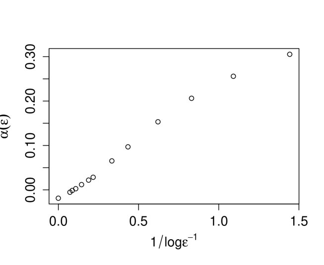
Figure 4. Simulated diapause example.

References

• [BCK+16] Jochen Blath, Adrián González Casanova, Noemi Kurt, Maite Wilke-Berenguer, et al. A new coalescent for seed-bank models. The Annals of Applied Probability, 26(2):857–891, 2016.
• [BK00] V. V. Buldygin and Yu. V. Kozachenko. Metric characterization of random variables and random processes, volume 188 of Translations of Mathematical Monographs. American Mathematical Society, Providence, RI, 2000. Translated from the 1998 Russian original by V. Zaiats.
• [CL91] Dan Cohen and Simon A Levin. Dispersal in patchy environments: the effects of temporal and spatial structure. Theoretical Population Biology, 39(1):63–99, 1991.
• [Coh66] Dan Cohen. Optimizing reproduction in a randomly varying environment. Journal of theoretical biology, 12(1):119–129, 1966.
• [Coh79] Joel E. Cohen. Ergodic theorems in demography. Bulletin of the American Mathematical Society, 1:275–95, 1979.
• [Col54] L.C. Cole. The Population Consequences of Life History Phenomena. The Quarterly Review of Biology, 29(2):103, 1954.
• [DH83] B Derrida and HJ Hilhorst. Singular behaviour of certain infinite products of random 2$\times$ 2 matrices. Journal of Physics A: Mathematical and General, 16(12):2641, 1983.
• [EE00] Michael R Easterling and Stephen P Ellner. Dormancy strategies in a random environment: comparing structured and unstructured models. Evolutionary Ecology Research, 2(4):387–407, 2000.
• [EKM97] Paul Embrechts, Claudia Klüppelberg, and Thomas Mikosch. Modelling extremal events, volume 33 of Applications of Mathematics (New York). Springer-Verlag, Berlin, 1997.
• [HMTŽ18] Lukas Heinrich, Johannes Mueller, Aurelien Tellier, and Daniel Živković. Effects of population-and seed bank size fluctuations on neutral evolution and efficacy of natural selection. Theoretical population biology, 2018.
• [Kar82] Samuel Karlin. Classifications of selection migration structures and conditions for a protected polymorphism. Evolutionary biology, 14:61–204, 1982.
• [Pol90] David Pollard. Empirical Processes: Theory and Applications, volume 2 of CBMS-NSF Regional Conference Series in Probability and Statistics. Institute of Mathematical, Hayward, California, 1990.
• [SL18] William R Shoemaker and Jay T Lennon. Evolution with a seed bank: The population genetic consequences of microbial dormancy. Evolutionary applications, 11(1):60–75, 2018.
• [ST18] David Steinsaltz and Shripad Tuljapurkar. Stochastic growth rates for populations in random environments with rare migration. 2018.
• [Teu75] Jozef L Teugels. The class of subexponential distributions. The Annals of Probability, pages 1000–1011, 1975.
• [TI93] Shripad Tuljapurkar and Conrad Istock. Environmental uncertainty and variable diapause. Theoretical Population Biology, 43(3):251–280, 1993.
• [TW00] S. Tuljapurkar and P. Wiener. Escape in time: stay young or age gracefully? Ecological Modelling, 133(1-2):143–159, 2000.
• [WT94] P. Wiener and S. Tuljapurkar. Migration in variable environments: exploring life-history evolution using structured population models. Journal of Theoretical Biology, 166(1):75–90, 1994.