Stochastic growth rates for populations in random environments with rare migration

Abstract.

The growth of a population divided among spatial sites, with migration between the sites, is sometimes modelled by a product of random matrices, with each diagonal elements representing the growth rate in a given time period, and off-diagonal elements the migration rate. The randomness of the matrices then represents stochasticity of environmental conditions. We consider the case where the off-diagonal elements are small, representing a situation where migration has been introduced into an otherwise sessile meta-population. We examine the asymptotic behaviour of the long-term growth rate. When there is a single site with the highest growth rate, under the assumption of Gaussian log growth rates at the individual sites (or having Gaussian-like tails) we show that the behavior near zero is like a power of $\epsilon$, and derive upper and lower bounds for the power in terms of the difference in the growth rates and the distance between the sites. In particular, when the difference in mean log growth rate between two sites is sufficiently small, or the variance of the difference between the sites sufficiently large, migration will always be favored by natural selection, in the sense that introducing a small amount of migration will increase the growth rate of the population relative to the zero-migration case.

1. Introduction

1.1. Biological motivation

If a population is divided among spatial sites with distinct fixed growth rates, with no migration between sites, the numbers in the best site will become overwhelmingly larger than those at the other sites, and the overall population growth rate will be determined by the rate prevailing at the best site. Introducing migration between sites, as Karlin showed [Kar82], will always reduce the long-run growth rate of the total population.

Karlin’s theorem assumes deterministic growth. den Boer [dB68] argued that migration may increase long-run growth when there is independent or weakly correlated stochastic variation in growth among sites. But Cohen [Coh66] and Cohen and Levin [CL91] used analysis and simulations to show that long-run growth of a population could increase as a result of a life cycle delay when there are some kinds of random variation in time, or by migration when there are some kinds of random variation across space. These kinds of stochastic variation have been formulated as random matrix models whose Lyapunov exponent is the long-run growth rate of the population, as discussed by [TW00, WT94]. In this general setting, we would like to know whether the long-run growth rate increases when there is mixing in space and/or time [TW00] — biologically, when should migration and/or delay be favoured to evolve? A general and precise answer has been difficult because previous work [WT94] shows that the long-run growth rate can be singular (e.g., non-differentiable) in the limit of no mixing. A similar singularity arises in random-matrix models used in models of disordered matter [DH83].

In the companion paper [ST18] we consider a simple model of migration among multiple sites, where two or more sites have the same optimal average log growth rate. We show there that a small increase from zero migration to migration at a small rate $\epsilon$ is associated with an increase on the order of $1/\log\epsilon^{-1}$, a change that overwhelms any cost of migration that is on the order of $\epsilon$ itself. As discussed there, while such a specification strains credulity when our life-history story is of individuals migrating among independently varying sites or patches, it arises naturally when we turn from geographic to demographic structure, reinterpreting “sites” as age classes. Rare migration becomes, in this framework, rare diapause, a rare random delay in an otherwise deterministic life history.

In this paper we consider the more generic situation for migration, where there is a single optimal site, where the mean log growth rate is highest, and then one or more alternative sites where growth is slower on average. We show that, under some plausible conditions, the increase in population growth rate with migration at rate $\epsilon$ (from $\epsilon=0$) is approximately proportional to a power $\epsilon^{p}$. We can bound $p$, yielding conditions under which $p<1$, making small deviations from zero migration advantageous in spite of migration costs on the order of $\epsilon$. Our results complement the analysis in [ERSS12] of optimal migration rates for populations divided among sites with varying stochastic growth rates. There interacting diffusions are used to characterize the migration rate that maximizes the long-run stochastic growth rate.

1.2. Notation and basic assumptions

Suppose $D_{1},D_{2},\dots$ is an i.i.d.  sequence of $d\times d$ diagonal matrices, representing population growth rates at $d$ separate sites in a succession of times. We write $\xi_{t}^{(0)},\dots,\xi_{t}^{(d-1)}$ for the diagonal elements of $D_{t}$, and assume $X_{t}^{(i)}\mathrel{\mathop{\mathchar 58\relax}}=\log\xi_{t}^{(i)}$ all have finite mean $\mu_{i}$ and finite variance $\tau_{i}$. We order them so that $\mu_{0}$ is the largest. We also write $\tilde{\mu}^{(i)}\mathrel{\mathop{\mathchar 58\relax}}=\mu_{0}-\mu_{i}$. We assume that $\tilde{\mu}^{(i)}>0$ for all $i=1,\dots,d-1$.

We will be assuming throughout that $X_{t}^{(0)}$ is Gaussian with mean $\mu_{0}$ and variance $\tau^{(0)}<\infty$, and that for $j\geq 1$

$$\widetilde{X}_{t}^{(j)}\mathrel{\mathop{\mathchar 58\relax}}=X_{t}^{(j)}-X_{t}^{(0)},$$

is Gaussian with mean $-\tilde{\mu}^{(j)}$ and variance $\tau^{(j)}<\infty$. This assumption is made to simplify the notation in the proofs. It would suffice to assume these variables to be sub-Gaussian, in which case different versions of the sub-Gaussian variance factor would appear in the upper and lower bounds. The notation for sub-Gaussian random variables, and the appropriate modification of the main result, are outlined briefly in section 6.

We write $\mathbf{X}$ for the complete collection of all $X^{(j)}_{t}$ for $j=0,1,\dots,d-1$, $0\leq t<\infty$.

We define the migration graph $\mathcal{M}$ to be a simple and irreducible directed graph whose vertices are the sites $\{0,\dots,d-1\}$, representing the transitions that have nonzero probability. We let $A_{t}$ be an i.i.d. sequence of nonnegative $d\times d$ matrices with zeros on the diagonal, representing migration rates in time-interval $t$. We follow the convention from the matrix population model literature, that transition rates from state $i$ to state $j$ are found in matrix entry $(j,i)$. Population distributions are thus naturally column vectors, and are updated from time $t-1$ to time $t$ by left multiplication.

We assume $A_{t}(j,i)$ are bounded above almost surely. We assume that if $i\nrightarrow j$ then $A_{t}(j,i)$ is identically 0, while for $i\rightarrow j$

$$\mathbb{E}\bigl{[}A_{t}(j,i)\,\bigl{|}\,D_{t}\bigr{]}$$

is bounded below almost surely. We assume that the collection of pairs $(D_{t},A_{t})_{t=0}^{\infty}$ is jointly independent, but note that we do not assume for a given $t$ that $A_{t}$ and $D_{t}$ are independent, only that there is a lower bound to how close $A_{t}(j,i)$ can come to 0 that is independent of all $D_{t}$.

We let $\Delta_{t}$ be a random diagonal matrix with entries $\Delta_{t}^{0},\dots,\Delta_{t}^{d-1}$. (Generally we will be thinking of $\Delta$ as the growth or survival penalty for migration, so that the entries will be negative, but this is not essential.) We assume the penalty acts multiplicatively on growth — this seems reasonable from a modeling perspective, and avoids the problem of negative matrix entries — and is proportional to $\epsilon$. We assume that these penalties are almost surely bounded, with $\|\Delta\|\mathrel{\mathop{\mathchar 58\relax}}=\max_{i,j}\operatorname{ess}\sup\bigl{|}\Delta_{t}^{i}-\Delta_{t}^{j}\bigr{|}<\infty.$

We define

$$D_{t}(\epsilon)\mathrel{\mathop{\mathchar 58\relax}}=\mathrm{e}^{\epsilon\Delta}D_{t}+\epsilon A_{t}.$$

For $\epsilon>0$ the i.i.d.  sequence $D_{t}(\epsilon)$ satisfies the conditions for the existence of a stochastic growth rate independent of starting condition.[Coh79] That is, if we define the partial products

$$R_{T}(\epsilon)\mathrel{\mathop{\mathchar 58\relax}}=D_{T}(\epsilon)\cdot D_{T-1}(\epsilon)\cdot\cdots\cdot D_{1}(\epsilon)$$

then

$$a(\epsilon)\mathrel{\mathop{\mathchar 58\relax}}=\lim_{T\to\infty}T^{-1}\log R_{T}(\epsilon)_{ij}$$

are well defined deterministic quantities, in the sense that the limit exists almost surely, is almost-surely constant, and is the same for any $0\leq i,j\leq d-1$.

Of course, $R_{T}(0)$ is not so simple. The off-diagonal terms are all 0, while on the diagonal, by the Strong Law of Large Numbers,

$$\lim_{T\to\infty}T^{-1}\log R_{T}(0)_{ii}=\mu_{i}.$$

1.3. The effect of the penalty $\Delta$

We will mostly be concerned with analyzing the case $\Delta\equiv 0$. For most purposes, $\Delta$ has no effect. But this is not always true.

The crucial point is that the effect of $\Delta$ is always nearly linear in $\epsilon$, while the increase of $a$ near 0 is often superlinear, growing as $\epsilon^{\beta}$. If the power $\beta$ is strictly less than 1, the rapid increase in $a$ near 0 will be qualitatively unaffected by a linear term for $\epsilon$ sufficiently small. Even when the linear term is negative (as we will generally be assuming it to be), the growth rate $a$ will still be increasing on a small interval of $\epsilon>0$.

On the other hand, as discussed in section 1.4 in some cases we cannot exclude the possibility that the growth rate when $\Delta\equiv 0$ is qualitatively like $\epsilon^{\beta}$ with $\beta\geq 1$. If $\beta>1$ and $\Delta_{0}<0$ then $a$ will be decreasing near 0; if $\beta=1$ then a more sensitive analysis would be required.

Since the upper and lower bounds on the appropriate power of $\epsilon$ in Theorem 1 are distinct, with the lower bound on the growth rate (the upper bound on the power of $\epsilon$) being sometimes larger than 1, the current results will not always permit us to ascertain whether the growth rate increases or decreases for small increases in $\epsilon$.

1.4. Main result

If $d=2$ we have an upper bound that $a(\epsilon)-a(0)$ is smaller than $\epsilon^{4\tilde{\mu}^{(1)}/(2\tilde{\mu}^{(1)}+\tau^{(1)})}$, and lower bound $\epsilon^{4\tilde{\mu}^{(1)}/\tau^{(1)}}$. For $d>2$ this becomes slightly more complicated for two reasons: First, the growth will be dominated by one dimension that has the fastest growth; second, the increment to growth will be smaller if direct transition between the best two sites is impossible. For this purpose, for each $1\leq j\leq d-1$ we define $\kappa_{j}$ to be the smallest length of a cycle in $\mathcal{M}$ that starts and ends at 0, and passes through $j$. (Thus $\kappa_{j}\geq 2$, and is equal to 2 when $A(0,j)>0$ and $A(j,0)>0$ both with positive probability.) Define also

(1) $$\rho^{(j)}\mathrel{\mathop{\mathchar 58\relax}}=\frac{\tilde{\mu}^{(j)}}{\tau^{(j)}}\,.$$

The calculation of $\rho$ is illustrated in Figure 1.

$$\mathcal{M}$$

$\operatorname{Cov}(X_{t}^{(i)},X_{t}^{(j)})$

$$\blockarray{ccccc}&0123\\ \block{c(cccc)}01-0.50.70.5\\ 1-0.5100\\ 20.701-0.3\\ 30.50-0.32\\$$

$j$	$\mathbb{E}[X_{t}^{(j)}]$	$\tau^{(j)}$	$\rho^{(j)}$	$\kappa_{j}$
0	1
1	$0.4$	3	$0.2$	3
2	$0.7$	$0.6$	$0.5$	3
3	0	$2$	$0.5$	2

Figure 1. Calculating $\rho$ on a four-site graph. We see that both $\kappa\rho$ and $\kappa\rho/(1+2\rho)$ are minimized at site 1, despite the fact that it is not in the shortest cycle, nor does it have the smallest mean difference in log growth rate from the optimal site 0.

Theorem 1.

Under the assumptions of section 1.2, let $j$ be the site that minimises $\kappa_{j}\rho^{(j)}$, and $j^{\prime}$ the site that minimises $\kappa_{j^{\prime}}\rho^{(j^{\prime})}/(1+2\rho^{(j^{\prime})})$. If $\Delta_{0}=0$ then for any $c^{\prime}>0$ there are positive constants $C,C^{\prime}$ (depending on the $\kappa,\rho,\rho_{*},d,\mu_{A},\tau_{A}$) such that for all $\epsilon>0$ sufficiently small,

(2) $$\frac{C}{\log\epsilon^{-1}}\epsilon^{2\kappa_{j}\rho^{(j)}}\leq a(\epsilon)-a(0)\leq C^{\prime}\bigl{(}\epsilon\log\epsilon^{-1}\bigr{)}^{2\kappa_{j^{\prime}}\rho^{(j^{\prime})}/(1+2\rho^{(j^{\prime})})}(\log\epsilon^{-1})^{c^{\prime}}.$$

Suppose now $\mathbb{E}[\Delta_{0}]<0$. Then

• If $2\kappa_{j}\rho^{(j)}<1$ then both bounds in (2) still hold;

• If $\frac{2\kappa_{j^{\prime}}\rho^{(j^{\prime})}}{1+2\rho^{(j^{\prime})}}<1\leq 2\kappa_{j}\rho^{(j)}$ then the upper bound in (2) holds;

• If $\frac{2\kappa_{j^{\prime}}\rho^{(j^{\prime})}}{1+2\rho^{(j^{\prime})}}>1$ then $a$ is differentiable at $0$, with $a^{\prime}(0)=-\Delta_{0}$.

In the Appendix we discuss that the requirement for these

Note that $\rho^{(j)}=\infty$ when the distribution of $\xi_{t}^{(j)}$ is not heavy-tailed — for example, very natural choices such as gamma-distributed diagonal elements — making the lower bound on the left-hand side vacuous, but it remains an open question whether zero subvariance (see the Appendix for definitions) implies that the approach of $a(\epsilon)$ to 0 is faster than polynomial in $\epsilon$.

2. Excursion decompositions

Since we are assuming the unique maximum average growth rate is at site 0, the maximum growth for the perturbed process will arise from rare excursions away from 0; in particular, from those that include the (not necessarily unique) site that minimises $\rho\kappa$ in (1).

Define $\mathcal{E}$ to be the set — called the excursions from 0 — of cycles in the migration graph that start and end at 0, with no intervening returns to 0. For an excursion $\mathbf{e}$ we write $|\mathbf{e}|$ for the length of the cycle minus 2 — that is, the number of time steps spent away from 0.

For a given excursion $\mathbf{e}$ we define

$$K(\mathbf{e}) \mathrel{\mathop{\mathchar 58\relax}}=\bigl{\{}0\leq t\leq|\mathbf{e}|+1\,\mathrel{\mathop{\mathchar 58\relax}}\,\mathbf{e}_{t}\neq\mathbf{e}_{t+1}\bigr{\}}$$

$$\kappa(\mathbf{e}) \mathrel{\mathop{\mathchar 58\relax}}=\max\bigl{\{}\kappa_{j}\,\mathrel{\mathop{\mathchar 58\relax}}\,j\in\mathbf{e}\bigr{\}};$$

$$\rho(\mathbf{e}) \mathrel{\mathop{\mathchar 58\relax}}=\min\left\{\rho^{(j)}\,\mathrel{\mathop{\mathchar 58\relax}}\,j\in\mathbf{e}\right\}.$$

Note that 0 and $T$ are always in $K(\mathbf{e})$, and the definition of $\kappa_{j}$ implies that $\kappa(\mathbf{e})\leq\#K(\mathbf{e})$. We will refer to $\kappa(\mathbf{e})$ as the diameter of $\mathbf{e}$.

We write $\hat{\mathcal{E}}_{T}$ for the collection of sequences of excursions that can be fit into time $\{1,\dots,T\}$. That is, an element $\hat{\mathbf{e}}\in\hat{\mathcal{E}}_{T}$ has an excursion count $k(\hat{\mathbf{e}})$, such that each $i\in\{1,\dots,k(\hat{\mathbf{e}})\}$ there is a pair $(t_{i},\hat{\mathbf{e}}_{i})$ with $t_{i}\in\{2,\dots,T-1\}$ and $\hat{\mathbf{e}}_{i}\in\mathcal{E}$ satisfying

$$t_{i}+|\hat{\mathbf{e}}_{i}| <t_{i+1},$$

$$t_{k(\hat{\mathbf{e}})}+|\hat{\mathbf{e}}_{k(\hat{\mathbf{e}})}| \leq T.$$

We write the total length of an excursion sequence as

$$\|\hat{\mathbf{e}}\|\mathrel{\mathop{\mathchar 58\relax}}=\sum_{i=1}^{k(\hat{\mathbf{e}})}|\hat{\mathbf{e}}_{i}|.$$

We also write $\hat{\mathcal{E}}_{T;k,n,m}$ for the subset of $\hat{\mathcal{E}}_{T}$ comprising excursion sequences whose excursion count is $k$, whose total length is $n$, and the sum of whose change-point counts $\#K(\hat{\mathbf{e}}_{i})$ is $m$. The null excursion sequence is the element of $\hat{\mathcal{E}}_{T}$ with $k(\hat{\mathbf{e}})=\|\hat{\mathbf{e}}\|=0$. We illustrate an excursion sequence in Figure 2.

Figure 2. An excursion sequence for $T=70$ comprising $k=5$ excursions. This is based on the migration graph example from Figure 1. Three excursions (red) have diameter 3, and one (green) has diameter 2. Note that one timepoint ($t=21$) is included in two different excursions. The red excursions all have $\rho(\hat{\mathbf{e}})=0.2$, and the green excursion has $\rho(\hat{\mathbf{e}})=0.5$. The lengths are 6, 2, 3, 5, 5, giving the sequence a total length $n=21$. The change-point counts are 3, 2, 3, 3, 4, summing to $m=15$.

The $(0,0)$ entry of the product $R_{T}$ will be a sum of terms that are enumerated by elements of $\hat{\mathcal{E}}_{T}$, corresponding to paths through the sites. We define new random variables as a function of the realizations of $\mathbf{X}$ and of $\mathbf{A}$ (the collection of all matrices $A$)

(3) $$\alpha_{t}(i,j)\mathrel{\mathop{\mathchar 58\relax}}=\begin{cases}\log\epsilon+\log A_{t}(j,i)-X_{t}^{(0)}&\text{ if }i\neq j,\\ 0&\text{ if }i=j.\end{cases}$$

Given an excursion $\mathbf{e}$ and a starting time $t_{0}\in\{2,\dots,T-|\mathbf{e}|\}$ we define the random variables

(4) $$\begin{split}\mathbf{e}[t_{0};\mathbf{X},\mathbf{A}]&\mathrel{\mathop{\mathchar 58\relax}}=\sum_{t\in K(\mathbf{e})}\alpha_{t+t_{0}}(\mathbf{e}_{t},\mathbf{e}_{t+1})+\sum_{t\in\{1,\dots,|\mathbf{e}|\}\setminus K(\mathbf{e})}\widetilde{X}_{t+t_{0}}^{(\mathbf{e}_{t})}\,,\\ \mathbf{e}^{\Delta}[t_{0};\mathbf{X},\mathbf{A}]&\mathrel{\mathop{\mathchar 58\relax}}=-\sum_{t\in K(\mathbf{e})}\Delta_{t_{0}+t}+\sum_{t\in\{1,\dots,|\mathbf{e}|\}\setminus K(\mathbf{e})}\left(\Delta_{t}^{\mathbf{e}_{t}}-\Delta_{t}^{0}\right).\end{split}$$

Of course, this sum may be $-\infty$, if it includes a transition at which the corresponding entry of $A$ is 0. But the assumptions imply that it is finite with nonzero probability if $\mathbf{e}\in\mathcal{E}$. Given an excursion sequence $\hat{\mathbf{e}}=\bigl{(}(t_{i},\hat{\mathbf{e}}_{i})\bigr{)}_{i=1}^{k}\in\hat{\mathcal{E}}_{T}$, we define

(5) $$\hat{\mathbf{e}}[\mathbf{X},\mathbf{A}]\mathrel{\mathop{\mathchar 58\relax}}=\sum_{i=1}^{k}\hat{\mathbf{e}}_{i}^{\Delta}[t_{i};\mathbf{X},\mathbf{A}],\quad\text{ and }\hat{\mathbf{e}}[\mathbf{X},\mathbf{A}]\mathrel{\mathop{\mathchar 58\relax}}=\sum_{i=1}^{k}\hat{\mathbf{e}}^{\Delta}_{i}[t_{i};\mathbf{X},\mathbf{A}].$$

The quantity we are trying to approximate is

(6) $$a(\epsilon)-a(0)=\lim_{T\to\infty}T^{-1}\Bigl{(}\log R_{T}(\epsilon)_{0,0}-\sum_{i=1}^{T}X_{i}^{(0)}\Bigr{)}.$$

Lemma 2.

(7) $$\log R_{T}(0,0)=\sum_{t=1}^{T}X_{t}^{(0)}+\epsilon\sum_{t=1}^{T}\Delta_{t}^{0}+\log\Bigl{(}1+\sum_{\hat{\mathbf{e}}\in\hat{\mathcal{E}}_{T}\setminus\{\hat{\mathbf{e}}^{0}\}}\mathrm{e}^{\hat{\mathbf{e}}[\mathbf{X},\mathbf{A}]+\epsilon\hat{\mathbf{e}}^{\Delta}[\mathbf{X},\mathbf{A}]}\Bigr{)},$$

where $\hat{\mathbf{e}}^{0}$ is the null excursion sequence.

Proof.

We have, by definition,

$$R_{T}(0,0)=\sum_{(x_{0},\dots,x_{T})}\prod_{t=1}^{T}D_{t}(\epsilon)(x_{t},x_{t-1}),$$

where the summation is over $(x_{0},\dots,x_{T})\in\{0,\dots,d-1\}^{T+1}$ with $x_{0}=x_{T}=0$. Note that we may restrict the summation to $(T+1)$-tuples such that $D_{t}(\epsilon)(x_{t},x_{t-1})>0$, which will only be true when $(x_{t-1},x_{t})$ is an edge of $\mathcal{M}$. Such sequences of states map one-to-one onto excursion sequences. The product corresponding to excursion sequence $\hat{\mathbf{e}}=\bigl{(}(t_{i},\hat{\mathbf{e}}_{i})\bigr{)}_{i=1}^{k}$ is

(8) $$\prod_{i=1}^{k+1}\Bigl{(}\prod_{t=t_{i-1}+1}^{t_{i}}D_{t}(\epsilon)(0,0)\Bigr{)}\cdot\prod_{i=1}^{k}\Bigl{(}\prod_{t=1}^{|\hat{\mathbf{e}}_{i}|}D_{t+t_{i}}(\epsilon)\bigl{(}(\hat{\mathbf{e}}_{i})_{t},(\hat{\mathbf{e}}_{i})_{t+1}\bigr{)}\Bigr{)},$$

where $t_{0}=0$ and $t_{k+1}=T$.

We have $D_{t}(\epsilon)(0,0)=\mathrm{e}^{X_{t}^{0)}+\epsilon\Delta_{0}}$. Thus, we may write the log of the expression in (8) as

(9) $$\sum_{t=1}^{T}\bigl{(}X_{t}^{(0)}+\epsilon\Delta_{0}\bigr{)}-\sum_{i=1}^{k}\sum_{t=1}^{|\hat{\mathbf{e}}_{i}|}\log\frac{D_{t+t_{i}}(\epsilon)\bigl{(}(\hat{\mathbf{e}}_{i})_{t},(\hat{\mathbf{e}}_{i})_{t+1}\bigr{)}}{D^{*}_{t+t_{i}}(0,0)}$$

We note that

$$\log\frac{D_{t+t_{i}}(\epsilon)(j,j)}{D_{t+t_{i}}(\epsilon)(0,0)}=\widetilde{X}_{t+t_{i}}^{(j)}+\epsilon\left(\Delta_{t+t_{i}}^{j}-\Delta_{t+t_{i}}^{0}\right)$$

and for $j\neq j^{\prime}$,

$$\log\frac{D_{t+t_{i}}(\epsilon)(j,j^{\prime})}{D_{t+t_{i}}(\epsilon)(0,0)}=\log\epsilon A_{t}(j,j^{\prime})-X_{t}^{(0)}-\epsilon\Delta_{t+t_{i}}^{0}.$$

Since $K(\hat{\mathbf{e}}_{i})$ is precisely the set of $t$ such that $(\hat{\mathbf{e}}_{i})_{t}\neq(\hat{\mathbf{e}}_{i})_{t+1}$, this means that (9) is precisely the same as $\hat{\mathbf{e}}_{i}[t_{i};\mathbf{X},\mathbf{A}]$, which completes the proof. ∎

Thus

(10) $$\log R_{T}(0,0)-\epsilon\sum_{t=1}^{T}\Delta_{t}^{0}-\sum_{t=1}^{T}X_{t}^{(0)}\geq\max_{\hat{\mathbf{e}}\in\hat{\mathcal{E}}_{T}}\hat{\mathbf{e}}[\mathbf{X},\mathbf{A}]-\max_{\hat{\mathbf{e}}\in\hat{\mathcal{E}}_{T}}\hat{\mathbf{e}}^{\Delta}[\mathbf{X},\mathbf{A}],$$

and

(11) $$\begin{split}\log R_{T}(0,0)&-\epsilon\sum_{t=1}^{T}\Delta_{t}^{0}-\sum_{t=1}^{T}X_{t}^{(0)}\\ &\leq 3\log T+\max_{1\leq k,n,m\leq T}\Bigl{(}\log\#\hat{\mathcal{E}}_{T;k,n,m}+\max_{\hat{\mathbf{e}}\in\hat{\mathcal{E}}_{T;k,n,m}}\hat{\mathbf{e}}[\mathbf{X},\mathbf{A}]\Bigr{)}+\max_{\hat{\mathbf{e}}\in\hat{\mathcal{E}}_{T}}\hat{\mathbf{e}}^{\Delta}[\mathbf{X},\mathbf{A}].\end{split}$$

Combining this with (6) yields the bounds we will use:

(12) $$a(\epsilon)-a(0)\geq\liminf_{T\to\infty}T^{-1}\max_{\hat{\mathbf{e}}\in\hat{\mathcal{E}}_{T}}\hat{\mathbf{e}}[\mathbf{X},\mathbf{A}]-\epsilon\|\Delta\|,$$

and

(13) $$\begin{split}a(\epsilon)&-a(0)\leq\limsup_{T\to\infty}T^{-1}\max_{1\leq k,n,m\leq T}\Bigl{(}\log\#\hat{\mathcal{E}}_{T;k,n,m}+\max_{\hat{\mathbf{e}}\in\hat{\mathcal{E}}_{T;k,n,m}}\hat{\mathbf{e}}[\mathbf{X},\mathbf{A}]\Bigr{)}+\epsilon\|\Delta\|.\end{split}$$

3. Derivation of the upper bound

We prove the upper bound in (2). We may replace $A_{t}(i,j)$ by $A_{t}(i,j)\vee 1$ for any $(i,j)\in\mathcal{M}$, since decreasing $A_{t}$ can only decrease $a(\epsilon)-a(0)$. That is, we put a floor under those off-diagonal elements which are allowable migrations. This avoids the nuisance of having entries be sometimes 0, and an upper bound that holds under these conditions will hold a fortiori under the original conditions. Indeed, we may assume without loss of generality that all $A_{t}(j,i)=1$ identically for $i\neq j$, since $a(\epsilon)$ — the stochastic growth rate with the correct values of $A_{t}$ — is no larger than $a(A_{*}\epsilon;\mathbf{1})$, the stochastic growth rate where all values of $A_{t}$ are replaced by 1. This changes our upper bound only by a constant, which may be absorbed into the constant of the theorem. Thus, we will proceed under this assumption.

An element of $\hat{\mathcal{E}}_{T;k,n,m}$ may be determined by the following choices:

1. Choose $k$ points out of $T$ where the excursions begin, yielding no more than $\binom{T}{k}$ possibilities;

2. Choose $k$ numbers for the lengths of the excursions that add up to $n$, yielding no more than $\binom{n}{k}$ possibilities;

3. Choose $m-2k$ timepoints within these excursions as times when there is a change of site, yielding at most $\binom{n}{m-2k}$ possibilities;

4. There are no more than $d^{m}$ ways to choose the sites to which the excursions move at the $m$ times when there is a change.

A crude bound based on Stirling’s Formula is

$$\log\binom{a}{b}\leq b+b\log\frac{a}{b},$$

which holds for all positive integers $b$ and $0\leq a\leq b$, as long as we adopt the convention $0\cdot\log 0=0\cdot\log\infty=0$. Then

(14) $$\log\#\hat{\mathcal{E}}_{T;k,n,m}\leq m\log d+(m-2k)\log\frac{n}{m-2k}+k\log\frac{n}{k}+T\log\frac{T}{k}.$$

Claim 3.

Suppose that $\rho_{j}$ and $\kappa_{j}$ are each minimised at site $j=1$. For any positive $c^{\prime}>0$, and any

$$z\geq\bigl{(}\epsilon\log\epsilon^{-1}\bigr{)}^{2\kappa_{1}\rho_{1}/(1+2\rho_{1})}\cdot(\log\epsilon^{-1})^{c^{\prime}},$$

we have

(15) $$\limsup_{T\to\infty}T^{-1}\log\mathbb{P}\bigl{\{}\max_{\hat{\mathbf{e}}\in\hat{\mathcal{E}}_{T;k,n,m}}\bigl{(}\hat{\mathbf{e}}[\mathbf{X},\mathbf{1}]+\log\#\hat{\mathcal{E}}_{T;k,n,m}\bigr{)}\geq zT\bigr{\}}<0$$

for all $\epsilon>0$ sufficiently small.

We prove this claim in section 5, and proceed here under this assumption. This means that

$$\sum_{T=T_{0}}^{\infty}\mathbb{P}\left\{T^{-1}\max_{1\leq k,n,m\leq T}\Bigl{(}\log\#\hat{\mathcal{E}}_{T;k,n,m}+\max_{\hat{\mathbf{e}}\in\hat{\mathcal{E}}_{T;k,n,m}}\hat{\mathbf{e}}[\mathbf{X},\mathbf{A}]\Bigr{)}\geq z\right\}<\infty.$$

By the Borel–Cantelli Lemma, this implies that with probability 1 this event occurs only finitely often. It follows that the limsup is smaller than $z$ almost surely, and hence, by (13), that

(16) $$a(\epsilon)-a(0)\leq\bigl{(}\epsilon\log\epsilon^{-1}\bigr{)}^{2\kappa_{1}\rho_{1}/(1+2\rho_{1})}\cdot(\log\epsilon^{-1})^{c^{\prime}}.$$

It remains only to clear away the assumption that that $\kappa_{j}$ and $\rho_{j}$ are both minimized at site 1. We do this by stratifying the excursions further by their diameter (recall the definition from section 2). Define

$$\breve{\rho}(\kappa)\mathrel{\mathop{\mathchar 58\relax}}=\min\bigl{\{}\rho_{j}\,\mathrel{\mathop{\mathchar 58\relax}}\,\kappa_{j}\leq\kappa\bigr{\}}.$$

If $\mathbf{e}$ is an excursion with diameter $\kappa$, then any site $j$ included in $\mathbf{e}$ has $\kappa_{j}\leq\kappa$, hence also $\rho_{j}\geq\breve{\rho}(\kappa)$. Furthermore,

(17) $$\min_{1\leq j\leq d-1}2\rho_{j}\kappa_{j}/(1+2\rho_{j})=\min_{2\leq\kappa\leq d-1}2\rho(\kappa)\kappa/(1+2\rho(\kappa))$$

The maximum in (13) may be written as a maximum over $(k_{2},\dots,k_{d-1})$, representing the number of excursions whose diameter is $2,3,\dots,d-1$, with the constraint $\sum k_{\kappa}=k$. We write $\hat{\mathcal{E}}_{T;k,n,m}^{(\kappa)}$ for the excursion sequences consisting of $k$ excursions, all of which have diameter $\kappa$; and $\hat{\mathcal{E}}_{T;(k_{\kappa}),n,m}$ for the set of excursion sequences that have exactly $k_{\kappa}$ excursions with diameter $\kappa$. Then $\hat{\mathcal{E}}_{T;(k_{\kappa}),n,m}$ naturally includes the direct sum of $\hat{\mathcal{E}}_{T;k_{\kappa},n,m}^{(\kappa)}$. (A sequence of mixed diameters $\hat{\mathbf{e}}\in\hat{\mathcal{E}}_{T;(k_{\kappa}),n,m}$ may be decomposed into sequences $\hat{\mathbf{e}}_{(\kappa)}\in\hat{\mathcal{E}}_{T;k_{\kappa},n,m}^{(\kappa)}$ of excursions with each particular diameter. Referring back to the example in Figure 2, this would entail making one excursion sequence by dropping out the green excursions, and a separate one by dropping out the red excursions.) Thus

$$\max_{\hat{\mathbf{e}}\in\hat{\mathcal{E}}_{T;k,n,m}}\hat{\mathbf{e}}[\mathbf{X},\mathbf{A}] =\max_{\sum k_{\kappa}=k}\>\max_{\hat{\mathbf{e}}\in\hat{\mathcal{E}}_{T;(k_{\kappa}),n,m}}\hat{\mathbf{e}}[\mathbf{X},\mathbf{A}]$$

$$\leq\max_{\sum k_{\kappa}=k}\>\max_{\hat{\mathbf{e}}_{(\kappa)}\in\hat{\mathcal{E}}_{T;k_{\kappa},n,m}^{(\kappa)}}\sum_{\kappa}\hat{\mathbf{e}}_{(\kappa)}[\mathbf{X},\mathbf{A}]$$

$$\leq\sum_{\kappa}\max_{1\leq k_{\kappa}\leq T}\>\max_{\hat{\mathbf{e}}_{(\kappa)}\in\hat{\mathcal{E}}_{T;k_{\kappa},n,m}^{(j)}}\hat{\mathbf{e}}_{(\kappa)}[\mathbf{X},\mathbf{A}],$$

using the general fact that the maximum of a sum is smaller than the sum of maxima. Thus we have

$$\max_{1\leq k,n,m\leq T}\Bigl{(}\log\#\hat{\mathcal{E}}_{T;k,n,m}+\max_{\hat{\mathbf{e}}\in\hat{\mathcal{E}}_{T;k,n,m}}\hat{\mathbf{e}}[\mathbf{X},\mathbf{A}]\Bigr{)} \leq\sum_{\kappa}\max_{1\leq k_{\kappa},n_{\kappa},m_{\kappa}\leq T}\>\max_{\hat{\mathbf{e}}_{(\kappa)}\in\hat{\mathcal{E}}_{T;k_{\kappa},n_{\kappa},m_{\kappa}}^{(\kappa)}}\hat{\mathbf{e}}_{(\kappa)}[\mathbf{X},\mathbf{A}].$$

Because all excursions in $\hat{\mathcal{E}}_{T;k_{\kappa},n_{\kappa},m_{\kappa}}^{(\kappa)}$ pass through only sites $j$ with $\rho_{j}\geq\breve{\rho}(\kappa)$, the same argument used for the upper bound in (16) may be applied to show that almost surely

$$\limsup_{T\to\infty}T^{-1}\max_{1\leq k_{\kappa},n_{\kappa},m_{\kappa}\leq T}\>\max_{\hat{\mathbf{e}}_{(\kappa)}\in\hat{\mathcal{E}}_{T;k_{\kappa},n_{\kappa},m_{\kappa}}^{(\kappa)}}\hat{\mathbf{e}}_{(\kappa)}[\mathbf{X},\mathbf{A}]\leq c_{\kappa}(\log\epsilon^{-1})^{c^{\prime}_{\kappa}}\epsilon^{2\kappa\breve{\rho}(\kappa)/(1+2\breve{\rho}(\kappa))}.$$

It follows that for $c\mathrel{\mathop{\mathchar 58\relax}}=(d-2)\cdot\max c_{\kappa}$ and $c^{\prime}\mathrel{\mathop{\mathchar 58\relax}}=\max c^{\prime}_{\kappa}$,

$$\limsup_{T\to\infty}T^{-1}\max_{1\leq k,n,m\leq T}\Bigl{(}\log\#\hat{\mathcal{E}}_{T;k,n,m}+ \max_{\hat{\mathbf{e}}\in\hat{\mathcal{E}}_{T;k,n,m}}\hat{\mathbf{e}}[\mathbf{X},\mathbf{A}]\Bigr{)}$$

$$\leq\sum_{\kappa}c_{\kappa}(\log\epsilon^{-1})^{c^{\prime}_{\kappa}}\epsilon^{2\kappa\breve{\rho}(\kappa)/(1+2\breve{\rho}(\kappa))}$$

$$\leq c(\log\epsilon^{-1})^{c^{\prime}}\epsilon^{\min_{1\leq j\leq d-1}2\kappa_{j}\rho_{j}/(1+2\rho_{j})}$$

by (17), which completes the proof.

4. Derivation of the lower bound

We show that the upper bound applies for each $j$; it will then hold in particular for the $j$ at which $\kappa_{j}\rho_{j}$ attains its minimum. We may assume without loss of generality that this optimal site is $j=1$, and we will write simply $\kappa$, $\tilde{\mu}$, and $\rho$ for $\kappa_{1}$, $\tilde{\mu}^{(1)}$, and $\rho_{1}$.

Let $0=j_{0},j_{1},j_{2},\dots,j_{I}=1,j_{I+1},\dots,j_{\kappa-1},j_{\kappa}=0$, be a cycle from 0 in $\mathcal{M}$, passing through 1. We may fix a real number $A_{*}$ and $p>0$ such that

(18) $$\mathbb{P}\Bigl{\{}\sum_{i=0}^{\kappa-1}\bigl{(}\log X_{t}^{(0)}-\log A_{t+i}(j_{i},j_{i+1})\bigr{)}<\kappa A_{*}\,\Bigm{|}\,\mathcal{D}\,\Bigr{\}}\geq p\text{ almost surely},$$

where $\mathcal{D}$ is the sigma-algebra generated by all the matrices $D_{t}(0)$.

Assume that $\epsilon\leq\mathrm{e}^{-1}$ and $T>\log\epsilon^{-1}$. Defining $k=\lfloor T/m\rfloor$ and $m=\lfloor\kappa\log\epsilon^{-1}/\tilde{\mu}\rfloor+\kappa$, we will apply (12) by considering only excursions of length exactly $m-1$, which proceed exactly through the sequence of sites $0=j_{0},j_{1},\dots,j_{I-1},1,\dots,1,j_{I+1},\dots,j_{\kappa-1},j_{\kappa}=0$, where site 1 is repeated exactly $m-\kappa+1$ times. The basic idea is that the excursion fills a time block of length $m$, proceeding as quickly as possible from 0 to 1, remaining as long as possible at 1, and then returning to 0.

We define the standard excursion $\mathbf{e}_{\circ}\mathrel{\mathop{\mathchar 58\relax}}=(j_{1},\dots,j_{I-1},1,\dots,1,j_{I+1},\dots,j_{\kappa-1})$, with $m-\kappa+1$ repetitions of site 1; and an excursion sequence $\hat{\mathbf{e}}_{\circ}$ consisting of those pairs $(\ell m+1,\mathbf{e}_{\ell})$ for which

(19) $$Y_{\ell}\mathrel{\mathop{\mathchar 58\relax}}=\mathbf{e}_{\circ}\bigl{[}\ell m+1;\mathbf{X},\mathbf{A}\bigr{]}>0.$$

That is, $\hat{\mathbf{e}}_{\circ}$ is put together from identical excursions of form $\mathbf{e}_{\circ}$ which can start only at times $\ell m+1$. Each one of the $k$ possible excursions is included precisely when its contribution to the sum would be positive.

We have

$$\hat{\mathbf{e}}[\mathbf{X},\mathbf{A}]=\sum_{\ell=0}^{k-1}(Y_{\ell})_{+}\,.$$

Since the excursion contributions $Y_{\ell}$ are all independent, combining (12) with the Strong Law of Large Numbers yields

(20) $$a(\epsilon)-a(0)\geq\frac{\mathbb{E}[(Y_{\ell})_{+}]}{m}-\epsilon\|\Delta\|.$$

We now observe that for any $\ell$

$$Y_{\ell}=\sum_{i=0}^{I-1}\alpha_{\ell m+i}(j_{i},j_{i+1})+\sum_{i=I}^{\kappa-1}\alpha_{(\ell+1)m-\kappa+i}(j_{i},j_{i+1})\,+\,\sum_{t=\ell m+I}^{(\ell+1)m-\kappa+I-1}\widetilde{X}_{t}^{(1)}.$$

Note that the $\alpha_{t}$ terms are independent of the $\widetilde{X}_{t}^{(1)}$ terms.

By (18), for any $y>0$,

$$\mathbb{P}\bigl{\{}Y_{\ell}>(m-\kappa+1)y\bigr{\}} \geq p\mathbb{P}\Bigl{\{}\left(\frac{\tilde{\mu}}{\rho}(m-\kappa+1)\right)^{1/2}Z>(m-\kappa+1)(y+\tilde{\mu})+\kappa\bigl{(}\log\epsilon^{-1}+A_{*}\bigr{)}\Bigr{\}}$$

$$\geq p\mathbb{P}\Bigl{\{}\left(\frac{\tilde{\mu}}{\rho}(m-\kappa+1)\right)^{1/2}Z>(m-\kappa+1)(y+2\tilde{\mu})+\kappa A_{*}\Bigr{\}}$$

$$\geq p\mathbb{P}\left\{Z>\left(\frac{m\rho}{\tilde{\mu}}\right)^{1/2}\left(y+\tilde{\mu}\left(2+\delta\right)\right)\right\},$$

where

$$Z\mathrel{\mathop{\mathchar 58\relax}}=\left(\frac{\tilde{\mu}}{\rho}(m-\kappa+1)\right)^{-1/2}\sum_{t=\ell m+I}^{(\ell+1)m-\kappa+I-1}(\widetilde{X}_{t}^{(1)}+\tilde{\mu})$$

is a standard Gaussian random variable and $\delta\mathrel{\mathop{\mathchar 58\relax}}=A_{*}/\log\epsilon^{-1}$. By Formula 7.1.13 of [AS65] we know that for all $z\geq 0$,

(21) $$\frac{\mathrm{e}^{-z^{2}/2}}{\geq}\frac{\mathrm{e}^{-z^{2}/2}}{2z+1}\geq\mathbb{P}\left\{Z>z\right\}\geq\frac{\mathrm{e}^{-z^{2}/2}}{2z+2}.$$

Hence for any $z_{*}>0$ we have

$$\mathbb{E}\left[\frac{(Y_{\ell})_{+}}{m-k+1}\right] =\int_{0}^{\infty}\mathbb{P}\bigl{\{}Y_{\ell}>(m-\kappa+1)y\bigr{\}}\operatorname{d\!}y$$

$$\geq\int_{0}^{\infty}p\mathbb{P}\left\{Z>\left(\frac{m\rho}{\tilde{\mu}}\right)^{1/2}\left(y+\tilde{\mu}\left(2+\delta\right)\right)\right\}\operatorname{d\!}y$$

$$\geq\frac{pz_{*}}{(4+2\delta)\tilde{\mu}+2z_{*}+2}\exp\left\{-\frac{m\rho}{2\tilde{\mu}}\left(z_{*}+\tilde{\mu}(2+\delta)\right)^{2}\right\}$$

Taking $z_{*}=1/(4+2\delta)m\rho$ yields

$$\mathbb{E}\left[\frac{(Y_{\ell})_{+}}{m-\kappa+1}\right] \geq\frac{p}{(25\tilde{\mu}+10)m\rho+2}\exp\left\{-\frac{1}{2}(2+\delta)^{2}m\rho\tilde{\mu}-1\right\}$$

$$\geq\frac{p\mathrm{e}^{-1-3\kappa\rho\tilde{\mu}}}{\kappa(1+\rho(25+10/\tilde{\mu})\log\epsilon^{-1})}\mathrm{e}^{2\kappa\rho(1+\delta/2)^{2}\log\epsilon}$$

$$\geq\frac{p\mathrm{e}^{-1-3\kappa\rho\tilde{\mu}}}{\kappa(1+\rho(25+10/\tilde{\mu})\log\epsilon^{-1})}\mathrm{e}^{2\kappa\rho(1+\delta/2)^{2}\log\epsilon}$$

$$\geq\frac{p\mathrm{e}^{-1-\kappa\rho(3\tilde{\mu}+5A_{*})}}{\kappa(1+\rho(25+10/\tilde{\mu})\log\epsilon^{-1})}\epsilon^{2\kappa\rho}$$

for $\epsilon$ sufficiently small that $\delta\leq 0.4$ and $m^{2}\rho^{2}\geq\frac{1}{8}$.

Combining this with (20), and assuming $\epsilon$ small enough that $\tilde{\mu}/\log\epsilon^{-1}<\frac{1}{2}$, we have $1-\kappa/m\geq\frac{1}{2}$ so

$$a(\epsilon)-a(0)\geq\frac{C}{\log\epsilon^{-1}}\epsilon^{2\kappa\rho}$$

where

$$C=\frac{p\mathrm{e}^{-1-\kappa\rho(3\tilde{\mu}+5A_{*})}}{2\kappa(1+\rho(25+5/\tilde{\mu})}.$$

5. Proof of Claim 3

Since the probability is decreasing in $z$, it will suffice to show the statement is true for

(22) $$z=\epsilon^{2\kappa_{1}\rho_{1}/(1+2\rho_{1})}\cdot(\log\epsilon^{-1})^{c^{\prime}},$$

where $c^{\prime}$ is any constant larger than $2\kappa_{1}$.

We define

$$\zeta\mathrel{\mathop{\mathchar 58\relax}}=\frac{k}{T},\quad\nu\mathrel{\mathop{\mathchar 58\relax}}=\frac{n}{k},\quad\beta\mathrel{\mathop{\mathchar 58\relax}}=\frac{m}{k}.$$

That is, $\zeta$ is the rate of excursions per unit time; $\nu$ is the average length of excursions; and $\beta$ is the average diameter of excursions. We have the constraints $1/\zeta\geq\nu\geq\beta\geq\kappa_{1}\geq 1$ (since $\kappa_{1}$ is the minimum $\kappa_{j}$, hence the minimum number of changes in each excursion). Then the bound (14) may be written as

(23) $$\log\#\hat{\mathcal{E}}_{T;k,n,m}\leq\zeta T\left(\beta\log d+(\beta-1)\log\nu-(\beta-2)\log(\beta-2)-\log\zeta\right).$$

Suppose now we fix some element $\hat{\mathbf{e}}$ of $\hat{\mathcal{E}}_{T;k,n,m}$, and list all the states of all the excursions in order as $j_{1},\dots,j_{n}$, we have

$$\mathbb{E}\bigl{[}\hat{\mathbf{e}}[\mathbf{X};\boldsymbol{1}]\bigr{]}\leq m\log\epsilon-\sum_{i=1}^{n}\tilde{\mu}^{(j_{i})}$$

and the random variable $Y\mathrel{\mathop{\mathchar 58\relax}}=\hat{\mathbf{e}}[\mathbf{X};\boldsymbol{1}]-\mathbb{E}[\hat{\mathbf{e}}[\mathbf{X};\boldsymbol{1}]]$ is Gaussian with variance bounded by $\sum_{i=1}^{n}\tau^{(j_{i})}$.

For any $x,z>0$, by (21)

$$\mathbb{P}\bigl{\{}\bigl{(}\hat{\mathbf{e}}[\mathbf{X},\boldsymbol{1}] +x\bigr{)}\geq zT\bigr{\}}\leq\mathbb{P}\Bigl{\{}Y\geq\sum_{i=1}^{n}\tilde{\mu}^{(j_{i})}+m\log\epsilon^{-1}+zT-x\Bigr{\}}$$

$$\leq\exp\biggl{\{}-\frac{1}{2}\left(\sum_{i=1}^{n}\tau^{(j_{i})}\right)^{-1}\left(\sum_{i=1}^{n}\tilde{\mu}^{(j_{i})}\,+\,m\log\epsilon^{-1}+zT-x\right)^{2}\biggr{\}}.$$

We are assuming that $\rho_{j}$ is minimized at $j=1$, $\tau^{(j_{i})}\leq\tilde{\mu}^{(j_{i})}/\rho_{1}$, so that

$$\log\mathbb{P}\bigl{\{}\bigl{(}\hat{\mathbf{e}}[\mathbf{X},\boldsymbol{1}] +x\bigr{)}\geq zT\bigr{\}}$$

$$\leq-\frac{1}{2}\left(\frac{1}{\rho_{1}}\sum_{i=1}^{n}\tilde{\mu}^{(j_{i})}\right)^{-1}\left(\sum_{i=1}^{n}\tilde{\mu}^{(j_{i})}+m\log\epsilon^{-1}+zT-x\right)^{2}.$$

Taking $x=\log\#\hat{\mathcal{E}}_{T;k,n,m}$ and substituting (23), we get

(24) $$\begin{split}\log\,\mathbb{P}\bigl{\{}&\max_{\hat{\mathbf{e}}\in\hat{\mathcal{E}}_{T;k,n,m}}\bigl{(}\hat{\mathbf{e}}[\mathbf{X},\boldsymbol{1}]+\log\#\hat{\mathcal{E}}_{T;k,n,m}\bigr{)}\geq zT\bigr{\}}\\ &\leq\log\#\hat{\mathcal{E}}_{T;k,n,m}+\max_{\hat{\mathbf{e}}\in\hat{\mathcal{E}}_{T;k,n,m}}\log\mathbb{P}\bigl{\{}\bigl{(}\hat{\mathbf{e}}[\mathbf{X},\boldsymbol{1}]+\log\#\hat{\mathcal{E}}_{T;k,n,m}\bigr{)}\geq zT\bigr{\}}\\ &\leq T\sup_{S\geq\kappa_{1}}\sup_{\beta\geq\kappa_{1}}\sup_{0\leq\zeta\leq 1}\zeta\biggl{[}\beta\log dS-\log\zeta-(\beta-2)\log(\beta-2)\\ &\hskip 28.45274pt-\frac{\rho_{1}}{2S}\biggl{(}S+\log\zeta+\frac{z}{\zeta}+(\beta-2)\log(\beta-2)-\beta\log dS+\beta\log\epsilon^{-1}\Bigr{)}\biggr{)}^{2}\,\biggr{]},\end{split}$$

where

$$S\mathrel{\mathop{\mathchar 58\relax}}=k^{-1}\sum_{i=1}^{n}\tilde{\mu}^{(j_{i})}\geq\nu\tilde{\mu}_{*}\geq\beta\tilde{\mu}_{*}\geq\kappa_{1}\tilde{\mu}_{*}$$

and $\tilde{\mu}_{*}\mathrel{\mathop{\mathchar 58\relax}}=\min_{j}\tilde{\mu}^{(j)}$. Our assumptions ensure that $\tilde{\mu}_{*}>0$.

We need to show that this supremum is strictly negative. We write this as $\sup\frac{z}{u}\Theta$, where $u=z/\zeta$ and

(25) $$\begin{split}\Theta=&\Theta(S,\beta,u)\\ \mathrel{\mathop{\mathchar 58\relax}}=&-\frac{\rho_{1}}{2S}\left(S+\beta\log\epsilon^{-1}+\log z+(\beta-2)\log(\beta-2)-\beta\log dS-\log u+u\right)^{2}\\ &\hskip 56.9055pt-\log z-(\beta-2)\log(\beta-2)+\beta\log dS+\log u.\end{split}$$

Here we have taken advantage of the fact that $\log\zeta<0$.

We will now show that there are positive constants $C$, $\Theta_{0}$, and $\epsilon_{0}$ (expressible in terms only of $c^{\prime},\rho_{1},\kappa_{1},\mu_{*},d$, such that for any fixed $\epsilon\in(0,\epsilon_{0})$,

$$z=\epsilon^{2\kappa_{1}\rho_{1}/(1+2\rho_{1})}(\log\epsilon^{-1})^{c^{\prime}},$$

and any $S\geq 1$, $\beta\geq\kappa_{1}$, and $u\geq 0$,

$$\Theta(S,\beta,u)\leq-\Theta_{0}-Cu.$$

The result then follows immediately, since then for all $T$,

$$T^{-1}\log\,\mathbb{P}\bigl{\{}\max_{\hat{\mathbf{e}}\in\hat{\mathcal{E}}_{T;k,n,m}}\bigl{(}\hat{\mathbf{e}}[\mathbf{X},\boldsymbol{1}]+\log\#\hat{\mathcal{E}}_{T;k,n,m}\bigr{)}\geq zT\bigr{\}}\leq zT\sup_{S\geq 1}\sup_{\beta\geq\kappa_{1}}\sup_{u\geq 0}\frac{1}{u}\Theta(S,\beta,u)\leq-Cz.$$

We consider three different regions for the parameters:

1. $S>\log^{2}\epsilon$ and $\beta>\frac{dS}{\log^{2}dS}+2$;

2. $S>\log^{2}\epsilon$ and $\beta\leq\frac{dS}{\log^{2}dS}+2$;

3. $\tilde{\mu}_{*}\kappa_{1}\leq S\leq\log^{2}\epsilon.$

In range (i) we have,

$$(\beta-2)\log(\beta-2)-\beta\log dS\geq-2\log dS-2\beta\log\log\epsilon^{-1}.$$

For $\epsilon$ sufficiently small

$$\Theta \leq-\frac{\rho_{1}}{2S}\left(S+(\beta-2\kappa_{1})\log\epsilon^{-1}-2\beta\log\log\epsilon^{-1}-2\log dS+u-\log u\right)^{2}$$

$$\hskip 113.81102pt+2\kappa_{1}\log\epsilon^{-1}+2\log dS+2\beta\log\log\epsilon^{-1}+\log u$$

$$\leq-\frac{\rho_{1}}{2}\left(\log^{2}\epsilon^{-1}-8\log\log\epsilon^{-1}\right)-\frac{\rho_{1}}{2}u-\beta\left(\rho_{1}\log\epsilon^{-1}-4\log\log\epsilon^{-1}-2\kappa_{1}\right)+(\rho_{1}+1)\log\left(\frac{2\rho_{1}+2}{\mathrm{e}\rho_{1}}\right)+(\rho_{1}+2)\log d$$

$$\leq-\frac{\rho_{1}}{3}\log^{2}\epsilon^{-1}-\frac{\rho_{1}}{2}u$$

for $\epsilon$ sufficiently small.

In the range (ii)

$$\Theta \leq-\frac{\rho_{1}}{2S}\left(S-\frac{dS}{\log dS}-\kappa_{1}\log\epsilon^{-1}+u-\log u\right)^{2}+\frac{dS}{\log dS}+\kappa_{1}\log\epsilon^{-1}+\log u$$

$$\leq-\log^{2}\epsilon^{-1}\left(\frac{\rho_{1}}{2}-\frac{(\rho_{1}+1)d}{\log\log\epsilon^{-1}}\right)-\frac{\rho_{1}}{2}u+\kappa_{1}(\rho_{1}+1)\log\epsilon^{-1}+(\rho_{1}+1)\log\left(\frac{2\rho_{1}+2}{\mathrm{e}\rho_{1}}\right)$$

$$\leq-\frac{\rho_{1}}{3}\log^{2}\epsilon^{-1}-\frac{\rho_{1}}{2}u$$

for $\epsilon$ sufficiently small.

In the range (iii) we rewrite $\Theta$ as

$$\Theta=-\frac{\rho_{1}}{2S}\left(y+S\right)^{2}-y+\beta\log\epsilon^{-1}+u,$$

where

$$y\mathrel{\mathop{\mathchar 58\relax}}=\beta\log\epsilon^{-1}+\log z+(\beta-2)\log(\beta-2)-\beta\log dS-\log u+u.$$

We note that

$$y \geq-\beta\log dS+(\beta-\kappa_{1})\log\epsilon^{-1}+c^{\prime}\log\log\epsilon^{-1}+u-\log u$$

$$\geq\left(u-\log u\right)+(c^{\prime}-2\kappa_{1})\log\log\epsilon^{-1}-\kappa_{1}\log d\tilde{\mu}_{*}$$

$$\hskip 28.45274pt+(\beta-\kappa_{1})\left(\log\epsilon^{-1}-\log\log\epsilon^{-1}-\log d\tilde{\mu}_{*}\right)$$

$$\geq 0$$

for $\epsilon$ sufficiently small. Applying the AM–GM inequality to the first term, we see that

$$\Theta \leq-(2\rho_{1}+1)y+\beta\log\epsilon^{-1}+u$$

$$\leq-2\rho_{1}\beta\log\epsilon^{-1}-\rho_{1}u-(2\rho_{1}+1)\log z$$

$$\hskip 85.35826pt+(2\rho_{1}+1)\left[\log\left(1+\frac{1}{2\rho_{1}}\right)-(\beta-2)\log(\beta-2)+\beta\log dS\tilde{\mu}_{*}\right]$$

$$\leq-\rho_{1}u-(\beta-\kappa_{1})\left(2\rho_{1}\log\epsilon^{-1}-(2\rho_{1}+1)\log d\log^{2}\epsilon^{-1}\right)$$

$$\hskip 85.35826pt-(2\rho_{1}+1)\left[(c^{\prime}-2\kappa_{1})\log\log\epsilon^{-1}-\mathrm{e}^{-1}-\log\left(1+\frac{1}{2\rho_{1}}\right)\right].$$

The last term on the right-hand side is negative for $\epsilon$ sufficiently small (and goes to $-\infty$ as $\epsilon\to 0$); the same is true of the second term unless $\beta=\kappa_{1}$, in which case that term is 0.

6. Sub-Gaussian log growth rates

In our analysis of the case of migration where the optimal site is unique, we have assumed that our log growth rates are Gaussian. This is for convenience, simplifying the notation. In fact, the results depend only on the asymptotic tail behavior. In this section we outline the modifications that are required for the extension to the sub-Gaussian case.

In [BLM13] a random variable $Z$ is said to be sub-Gaussian if it has finite variance factor $\tau(Z)$, defined as

(26) $$\tau^{*}(Z)\mathrel{\mathop{\mathchar 58\relax}}=\inf\left\{c\geq 0\,\mathrel{\mathop{\mathchar 58\relax}}\,\mathbb{E}\left[\mathrm{e}^{\lambda Z}\right]\leq\mathrm{e}^{c\lambda^{2}/2}\,\forall\lambda\in\mathbb{R}\right\}.$$

(The square-root of this is called the sub-Gaussian standard in [BK00].) This may be thought of as an upper bound on the scale of the tails, and it is this that determines the lower bound on the sensitivity of $a$. That is, in Theorem 1 the upper bounds still hold when the assumption that $\widetilde{X}_{t}^{(j)}$ is Gaussian with variance $\tau$ is replaced by sub-Gaussian with variance factor $\tau^{*}$.

Similarly, the lower bound on $a(\epsilon)$ only depends on a Gaussian lower bound on the tails

(27) $$\tau_{*}(Z)\mathrel{\mathop{\mathchar 58\relax}}=\liminf_{z\to\infty}\frac{z^{2}}{-2\log\mathbb{P}\bigl{\{}Z>z\bigr{\}}}$$

being nonzero. That is, in Theorem 1 the upper and lower bounds still hold when the assumption Gaussian with variance $\tau$ is replaced by $\tau^{*}$ and $\tau_{*}$ respectively.

We point out here that the assumption that $\widetilde{X}_{t}=\log(\xi_{t}^{(1)}/\xi_{t}^{(0)})$ have nonzero $\tau_{*}$ implies what may be considered exceptionally heavy tails for the growth rates — effectively, something like log-normal. This is what is required for a nontrivial lower bound in Theorem 1. Thus, it seems plausible to infer that the population will obtain no long-term benefit from sending occasional individuals to a site with lower average growth, unless the low average growth is compensated by fat positive tails, meaning that there is a small chance of a very large payoff. (These nearly heavy tails may also be generated if $\xi_{t}^{(0)}$ puts too much probability near 0 — that is, a population crash.)

The proof of the lower bound can easily be generalized to the sub-Gaussian case, if we replace the specific calculation of tail probabilities based on the Gaussian distribution with a bound based on Cramér’s Theorem [DZ09, Theorem 2.2.3]. (The power in the lower bound would need to be increased by an arbitrarily small $\delta$.) The extension of the upper bound of Theorem 1 can be done with the methods of [Pol90] for bounding the tails of maxima in terms of the Orlicz norm. Letting $\Psi(x)=e^{x^{2}}/5$, the Orlicz norm $\|Z\|_{\Psi}$ for a centered random variable $Z$ is defined to be

(28) $$\|Z\|_{\Psi}\mathrel{\mathop{\mathchar 58\relax}}=\inf\{C\,\mathrel{\mathop{\mathchar 58\relax}}\,\mathbb{E}[\Psi(|Z|/C)]<1\}.$$

We present here some elementary results about Orlicz norms and their relationship to the sub-Gaussian variance factors.

Lemma 4.

A sub-Gaussian centered random variable $Z$ satisfies

(29) $$\|Z\|_{\Psi} \leq\sqrt{\frac{5\tau^{*}(Z)}{2}};$$

(30) $$\tau_{*}(Z) \leq\tau^{*}(Z)<\infty.$$

If $Z$ is Gaussian with mean 0 and variance $\sigma^{2}$ then

(31) $$\tau_{*}(Z)=\tau^{*}(Z)=\sigma^{2}.$$

Proof.

The statement (31) is trivial.

If $\tau^{*}=\tau^{*}(Z)$ is finite then for any $\lambda,z,\delta>0$,

$$\mathbb{P}\bigl{\{}|Z|>z\bigr{\}}\leq\mathrm{e}^{\frac{(\tau^{*}+\delta)\lambda^{2}}{2}-\lambda z}.$$

Taking $\lambda=z/(\tau^{*}+\delta)$, we have $\mathbb{P}\bigl{\{}|Z|>z\bigr{\}}\leq\mathrm{e}^{-z^{2}/2(\tau^{*}+\delta)}$, which implies

(32) $$\mathbb{P}\bigl{\{}|Z|>z\bigr{\}}\leq\mathrm{e}^{-z^{2}/2\tau^{*}},$$

since $\delta$ is arbitrary. This immediately proves (30).

Integrating by parts, we have for $C>\sqrt{2\tau}$,

$$\mathbb{E}\left[\mathrm{e}^{Z^{2}/C^{2}}\right] =1+\frac{2}{C^{2}}\int_{0}^{\infty}z\mathrm{e}^{z^{2}/C^{2}}\mathbb{P}\bigl{\{}|Z|>z\bigr{\}}$$

$$\leq 1+\frac{2}{C^{2}}\int_{0}^{\infty}z\mathrm{e}^{z^{2}/C^{2}}\mathrm{e}^{-z^{2}/2\tau^{*}}$$

$$=1+\frac{2\tau^{*2}}{C^{2}-2\tau^{*}}.$$

If $C=\sqrt{5\tau^{*}/2}$ then this bound is 5, proving (29). ∎

Since it is a norm, the Orlicz norm of an arbitrary sum of random variables is no greater than the sum of the Orlicz norms. For independent sub-Gaussian random variables $X_{1},\dots,X_{k}$ the variance factors are also sub-additive.

Lemma 5.

For any independent centered sub-Gaussian random variables $X_{1},\dots,X_{k}$,

(33) $$\tau^{*}\Bigl{(}\sum X_{i}\Bigr{)}\leq\sum\tau^{*}(X_{i}),$$

and

(34) $$\mathbb{P}\Bigl{\{}\Bigl{|}\sum X_{i}\Bigr{|}>x\Bigr{\}}\leq\exp\Bigl{\{}-\left(2\sum\tau^{*}(X_{i})\Bigr{)}^{-1}x^{2}\right\}.$$

Also

(35) $$\|X_{1}+\cdots+X_{k}\|_{\Psi}\leq\sqrt{5/2}\left(\sum\tau^{*}(X_{i})\right)^{1/2}.$$

If $\max\tau^{*}(X_{i})\leq\tau$ then

(36) $$\mathbb{P}\Bigl{\{}\Bigl{|}\sum X_{i}\Bigr{|}>x\Bigr{\}}\leq\exp\left\{-\frac{x^{2}}{2k\tau}\right\}.$$

and

(37) $$\|X_{1}+\cdots+X_{k}\|_{\Psi}\leq\sqrt{\frac{5k}{2}\tau}.$$

Proof.

Statement (33) is Lemma 1.7 of [BK00], and (34) follows by (32). The remainder follows by Lemma 4. ∎

7. Simulations

We consider a $3\times 3$ example:

$$M_{t}(\mu,\sigma^{2})=\begin{pmatrix}e^{\sigma Z_{t}^{(0)}}&0&0\\ 0&e^{\sigma Z_{t}^{(1)}-0.1}&0\\ 0&0&e^{\sigma Z_{t}^{(2)}-0.2}\end{pmatrix},\qquad A_{t}(C)=\begin{pmatrix}0&C&1\\ 1&0&C\\ C&1&0\end{pmatrix},$$

with $Z_{t}^{(0)},Z_{t}^{(1)},Z_{t}^{(2)}$ i.i.d.  standard normal random variables, and $C$ is a nonnegative constant. If $C=0$ then the migration graph is a cycle of length 3, so $\kappa_{1}=\kappa_{2}=3$; if $C>0$ then $\kappa_{1}=\kappa_{2}=2$.

We consider three different cases for $(\sigma^{2},C)$: $I\mathrel{\mathop{\mathchar 58\relax}}(0.5,1)$, $II\mathrel{\mathop{\mathchar 58\relax}}(0.5,0)$, and $III\mathrel{\mathop{\mathchar 58\relax}}(1,1)$. We expect to find $\log a(\epsilon)/\log\epsilon^{-1}$ converging to a constant as $\epsilon\downarrow 0$. We have $\tilde{\mu}^{(1)}=0.1$ in all three cases. For cases I and II we have $\rho^{(1)}=0.1$, so that the power for case I is between

$$2\cdot 2\cdot 0.1=0.4\qquad\text{and}\qquad\frac{2\cdot 2\cdot 0.1}{1+2\cdot 0.1}=\frac{1}{3},$$

and for case II is between

$$2\cdot 3\cdot 0.1=0.6\qquad\text{and}\qquad\frac{2\cdot 3\cdot 0.1}{1+2\cdot 0.1}=0.5.$$

For case III $\rho^{(1)}$ is decreased to 0.05, so the power is between

$$2\cdot 2\cdot 0.05=0.2\qquad\text{and}\qquad\frac{2\cdot 2\cdot 0.05}{1+2\cdot 0.05}=\frac{2}{11}.$$

(Setting $\mu=0$ would put this into the setting of [ST18], with $a(\epsilon)$ behaving like $c/\log\epsilon^{-1}$ for some constant $c$, when $\epsilon$ is small.)

We plot some simulated results in Figures 3 through 5, plotting the $\log a(\epsilon)$ against $\log\epsilon^{-1}$. In the limit as $\epsilon\to 0$ this should approach a line whose slope is in the range given for the power of $\epsilon$ in Theorem 1. We plot lines with those slopes in each figure, and see that in the lowest range of $\epsilon$ (we take it down to $\epsilon=10^{-6}$) the slope comes down close to the upper limit, but is still higher. Of course, this is completely consistent with the true exponent being at the upper limit, particularly since we don’t know anything yet about how small $\epsilon$ would need to be before the asymptotic slope becomes apparent.

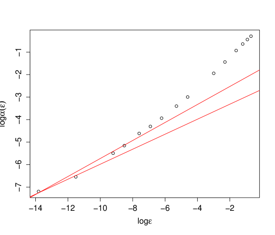
Figure 3. Simulated migration example with path length 2. The red lines have slope $0.4$ and $1/3$.

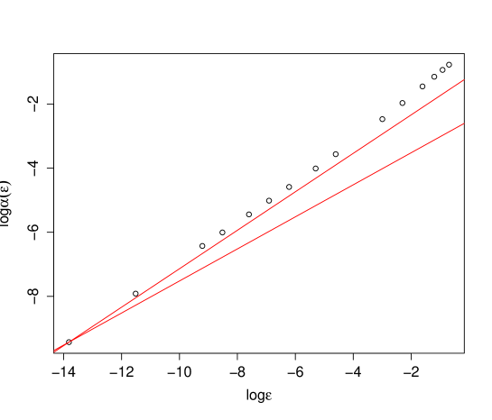
Figure 4. Simulated migration example with path length 3. The red lines have slope $0.5$ and $0.6$.

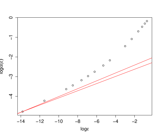
Figure 5. Simulated migration example with path length 2, and $\sigma^{2}=1$. The red lines have slope $0.2$ and $2/11$.

References

• [AS65] Milton Abramowitz and Irene Stegun. Handbook of mathematical functions, with formulas, graphs, and mathematical tables. Dover, New York, 1965.
• [BK00] V. V. Buldygin and Yu. V. Kozachenko. Metric characterization of random variables and random processes, volume 188 of Translations of Mathematical Monographs. American Mathematical Society, Providence, RI, 2000. Translated from the 1998 Russian original by V. Zaiats.
• [BLM13] Stéphane Boucheron, Gábor Lugosi, and Pascal Massart. Concentration Inequalities: A Nonasymptotic Theory of Independence. Oxford University Press, 2013.
• [CL91] Dan Cohen and Simon A Levin. Dispersal in patchy environments: the effects of temporal and spatial structure. Theoretical Population Biology, 39(1):63–99, 1991.
• [Coh66] Dan Cohen. Optimizing reproduction in a randomly varying environment. Journal of theoretical biology, 12(1):119–129, 1966.
• [Coh79] Joel E. Cohen. Ergodic theorems in demography. Bulletin of the American Mathematical Society, 1:275–95, 1979.
• [dB68] P. J. den Boer. Spreading of risk and stabilization of animal numbers. Acta biotheoretica, 18(1):165–194, 1968.
• [DH83] B Derrida and HJ Hilhorst. Singular behaviour of certain infinite products of random 2$\times$ 2 matrices. Journal of Physics A: Mathematical and General, 16(12):2641, 1983.
• [DZ09] A. Dembo and O. Zeitouni. Large Deviation Techniques and Applications. Springer Verlag, 2nd edition, 2009.
• [ERSS12] Steven N. Evans, Peter L. Ralph, Sebastian J. Schreiber, and Arnab Sen. Stochastic population growth in spatially heterogeneous environments. Jornal of Mathematical Biology, 66(3):423–76, February 2012.
• [Kar82] Samuel Karlin. Classifications of selection migration structures and conditions for a protected polymorphism. Evolutionary biology, 14:61–204, 1982.
• [Pol90] David Pollard. Empirical Processes: Theory and Applications, volume 2 of CBMS-NSF Regional Conference Series in Probability and Statistics. Institute of Mathematical, Hayward, California, 1990.
• [ST18] David Steinsaltz and Shripad Tuljapurkar. Stability of fixed life histories to perturbation by rare diapause. 2018.
• [TW00] S. Tuljapurkar and P. Wiener. Escape in time: stay young or age gracefully? Ecological Modelling, 133(1-2):143–159, 2000.
• [WT94] P. Wiener and S. Tuljapurkar. Migration in variable environments: exploring life-history evolution using structured population models. Journal of Theoretical Biology, 166(1):75–90, 1994.