Projective quantum Monte Carlo simulations guided by unrestricted neural network states

Abstract

We investigate the use of variational wave-functions that mimic stochastic recurrent neural networks, specifically, unrestricted Boltzmann machines, as guiding functions in projective quantum Monte Carlo (PQMC) simulations of quantum spin models. As a preliminary step, we investigate the accuracy of such unrestricted neural network states as variational Ansätze for the ground state of the ferromagnetic quantum Ising chain. We find that by optimizing just three variational parameters, independently on the system size, accurate ground-state energies are obtained, comparable to those previously obtained using restricted Boltzmann machines with few variational parameters per spin. Chiefly, we show that if one uses optimized unrestricted neural network states as guiding functions for importance sampling the efficiency of the PQMC algorithms is greatly enhanced, drastically reducing the most relevant systematic bias, namely that due to the finite random-walker population. The scaling of the computational cost with the system size changes from the exponential scaling characteristic of PQMC simulations performed without importance sampling, to a polynomial scaling, even at the ferromagnetic quantum critical point. The important role of the protocol chosen to sample hidden-spins configurations, in particular at the critical point, is analyzed. We discuss the implications of these findings for what concerns the problem of simulating adiabatic quantum optimization using stochastic algorithms on classical computers.

I Introduction

Quantum Monte Carlo (QMC) algorithms are generally believed to be capable of predicting equilibrium properties of quantum many-body systems at an affordable computational cost, even for relatively large system sizes, at least when the sign problem does not occur. However, it has recently been shown that the computational cost to simulate the ground state of a quantum Ising model with a simple projective QMC (PQMC) algorithm that does not exploit importance sampling techniques scales exponentially with the system size, making large-scale simulations unfeasible Inack et al. (2018). This happens in spite of the fact that the Hamiltonian is sign-problem free. PQMC methods have found vast use in condensed matter physics, in chemistry, and beyond (see, e.g., Refs. Ceperley and Alder (1986); Hammond et al. (1994); Foulkes et al. (2001); Carlson et al. (2015)). Shedding light on their computational complexity, and possibly improving it by using importance sampling techniques based on novel variational wave-functions, are therefore very important tasks. We address them in this Article.

PQMC algorithms have recently emerged as useful computational tools also to investigate the potential efficiency of adiabatic quantum computers in solving large-scale optimization problems via quantum annealing Finnila et al. (1994); Santoro et al. (2002); Boixo et al. (2014); Inack and Pilati (2015); Heim et al. (2015). In particular, it has been shown that the (stochastic) dynamics of simple PQMC simulations allows to tunnel through tall barriers of (effectively) double-well models even more efficiently than an adiabatic quantum computer which exploits incoherent quantum tunneling Isakov et al. (2016); Jiang et al. (2017); Mazzola et al. (2017); Inack et al. (2018). This result seems to suggest that there might be no systematic quantum speed-up in using a quantum annealing device to solve an optimization problem, compared to a stochastic QMC simulation performed on a classical computer Isakov et al. (2016). Remarkably, this computational advantage of the PQMC simulations with respect to the expected behavior of a quantum annealing device occurs also in more challenging models with frustrated couplings Inack et al. (2018), as in the recently introduced Shamrock model, where QMC algorithms based on the (finite temperature) path-integral formalism display instead an exponential slowdown of the tunneling dynamics Andriyash and Amin (2017). This result further stresses the importance of shedding light on the computational complexity of PQMC algorithms: if these computational techniques allowed one to simulate, with a polynomially scaling computational cost, both the ground-state properties of a model Hamiltonian, and also the tunneling dynamics of a quantum annealing device described by such Hamiltonian Inack et al. (2018), then the quantum speedup mentioned above would be very unlikely to be achieved. We focus in this paper on the first of the two aspects, specifically, on analyzing and improving the scaling of the computational cost to simulate ground-state properties of quantum Ising models.

It is well known that the efficiency of PQMC algorithms can be enhanced by implementing importance sampling techniques using as guiding functions accurate variational Ansätze Foulkes et al. (2001). However, building accurate variational wave-functions for generic many-body systems is a highly non trivial task. Recently, variational wave-functions that mimic the structure of neural networks have been shown to accurately describe ground-state properties of quantum spin and lattice models Carleo and Troyer (2017); Saito (2017); Saito and Kato (2018). The representational power and the entanglement content of such variational states, now referred to as neural network states, have been investigated Deng et al. (2017); Chen et al. (2018); Glasser et al. (2018); Gao and Duan (2017); Freitas et al. (2018), showing, among other properties, that they are capable of describing volume-law entanglement. The authors of Ref. Carleo and Troyer (2017) considered neural network states that mimic restricted Boltzmann machines (RBM), i.e. such that no interaction among hidden spins is allowed. One very appealing feature of such restricted neural network states is that the role of the hidden spins can be accounted for analytically, without the need of Monte Carlo sampling over hidden variables. Furthermore, such states provide very accurate ground-state energy predictions, which can be systematically improved by increasing the number of hidden spins per visible spin (later on referred to as hidden-spin density). However, this high accuracy is obtained at the cost of optimizing a number of variational parameters that increases with the system size. This optimization task can be tackled using powerful optimization algorithms such as the stochastic reconfiguration method (see, e.g, Ref. Sorella et al. (2007)). Yet, having to optimize a large number of variational parameters is not desirable in the context of quantum annealing simulations, since one would be dealing with a variational optimization problem, potentially even more difficult than the original classical optimization problem.

In this Article, we consider instead neural network states that mimic unrestricted Boltzmann machines (uRBMs), allowing intra-layer correlations among hidden spins, beyond the inter-layer hidden-visible correlations and the intra-layer visible-visible correlations (see Fig. 1). The structure of these states resembles the one of the shadow wave functions originally introduced to describe quantum fluids and solids Vitiello et al. (1988); Reatto and Masserini (1988). We test their representational power considering as a testbed the ferromagnetic quantum Ising chain. We find that by optimizing just three variational parameters, independently on the system size, very accurate ground-state energies are obtained, comparable to the case of restricted neural network states with one hidden spin per visible spin. Such a small number of variational parameters is a particularly appealing feature in the context of quantum annealing problems. However, it comes at the prize of having to perform Monte Carlo sampling over hidden-spin configurations.

The main goal of this Article is to show that the above-mentioned unrestricted neural network states can be used as a guide for importance sampling in PQMC simulations. This also implies that the development of neural network states can be limited to obtaining reasonably accurate, but not necessarily exact, variational Ansätze, since the residual error can be eliminated within the PQMC simulation. In particular, we provide numerical evidence that the major source of systematic bias of the PQMC algorithms, namely the bias originating from the finite size of the random-walker population which has to be stochastically evolved in any PQMC simulation, can be drastically reduced using optimized unrestricted neural network states, even at the point of changing the scaling of the required population size from exponential (corresponding to the case without importance sampling) to polynomial in the system size. This also implies a change of computational complexity from exponential to polynomial. For comparison, we show that a conventional variational wave-function of the Boltzmann type (with no hidden spins), instead, does not determine a comparable efficiency improvement.

The rest of the Article is organized as follows: in Section II we define the conventional Boltzmann-type variational wave functions and the unrestricted neural network states, and we then analyze how accurately they predict the ground-state energy of the quantum Ising chain via optimization of, respectively one and three, variational parameters. Section III deals with the continuous-time PQMC algorithm and with the implementation of importance sampling using both Boltzmann-type wave functions and, chiefly, unrestricted neural network states, showing how the systematic bias due to the finite random-walker population is affected, both at and away from the quantum critical point. The important effect of choosing different sampling protocols for the hidden spins is also analyzed. Our conclusions and the outlook are reported in Section IV.

II Unrestricted neural network states for quantum Ising models

In this article, we consider as a test bed the one-dimensional ferromagnetic quantum Ising Hamiltonian:

$$\hat{H}=\hat{H}_{\mathrm{cl}}+\hat{H}_{\mathrm{kin}},$$ (1)

where $\hat{H}_{\mathrm{cl}}=-J\sum_{i=1}^{N}{\sigma}^{z}_{i}{\sigma}^{z}_{i+1}$ and $\hat{H}_{\mathrm{kin}}=-\Gamma\sum_{i=1}^{N}{\sigma}^{x}_{i}$. $\sigma^{x}_{i}$, $\sigma^{y}_{i}$, and $\sigma^{z}_{i}$ indicate Pauli matrices acting on spins at the lattice site $i$. $N$ is the total number of spins, and we adopt periodic boundary conditions, i.e. ${\sigma}^{\alpha}_{N+1}={\sigma}^{\alpha}_{1}$, with $\alpha=x,y,z$. The parameter $J>0$ fixes the strength of the ferromagnetic interactions among nearest-neighbor spins. In the following, we set $J=1$. All energy scales are henceforth expressed in units of $J$. The parameter $\Gamma$ fixes the intensity of a transverse magnetic field. Given $\left|x_{i}\right>$ an eigenstate of the Pauli matrix ${\sigma^{z}_{i}}$ with eigenvalue $x_{i}=1$ when $\left|x\right>=\left|\uparrow\right>$ and $x_{i}=-1$ when $\left|x\right>=\left|\downarrow\right>$, the quantum state of $N$ spins is indicated by $\left|\mathit{\boldsymbol{x}}\right>=\left|x_{1}x_{2}...x_{N}\right>$. Notice that the function $E_{\mathrm{cl}}(\mathit{\boldsymbol{x}})=\langle\mathit{\boldsymbol{x}}|\hat{H}_{\mathrm{cl}}|\mathit{\boldsymbol{x}}\rangle$ (with $\mathit{\boldsymbol{x}}=\left(x_{1},x_{2},\dots,x_{N}\right)$) corresponds to the Hamiltonian function of a classical Ising model, while the operator $\hat{H}_{\mathrm{kin}}$ introduces quantum (kinetic) fluctuations.

Our first goal is to develop trial wave functions that closely approximate the ground state wave function $\Psi_{0}{(\mathit{\boldsymbol{x}})}=\left<\mathit{\boldsymbol{x}}|\Psi_{0}\right>$ of the Hamiltonian (1). A simple Ansatz can be defined as

$$\Psi_{\boldsymbol{\kappa}}{(\mathit{\boldsymbol{x}})}=e^{-\beta E_{\mathrm{cl}}({\mathit{\boldsymbol{x}}})}=e^{-K_{1}\sum_{i=1}^{N}x_{i}x_{i+1}}\;.$$ (2)

$\boldsymbol{\kappa}$ is here a set of real variational parameters to be optimized. Their values are obtained by minimizing the average of the energy, as in standard variational quantum Monte Carlo approaches. In this case, only one parameter $K_{1}=\beta$ is present, $\boldsymbol{\kappa}=\{K_{1}\}$. This choice is inspired by the classical Boltzmann distribution where $\beta$ would play the role of a fictitious inverse temperature. The above Ansatz will be referred to as Boltzmann-type wave function.

A more sophisticated Ansatz can be constructed by using a generative stochastic artificial neural network, namely an uRBM (see Fig. 1). Beyond the visible spin variables $\mathit{\boldsymbol{x}}=\left(x_{1},x_{2},\dots,x_{N}\right)$, one introduces $N$ hidden spin variables $\mathit{\boldsymbol{h}}=\left(h_{1},h_{2},\dots,h_{N}\right)$, taking values $h_{i}=\pm 1$ (with $i=1,\dots,N$). Periodic boundary conditions within the layers are also incorporated, i.e $x_{N+1}=x_{1}$ and $h_{N+1}=h_{1}$. The trial wave function is thus written in the following integral form:

$$\Psi_{\boldsymbol{\kappa}}(\mathit{\boldsymbol{x}})=\sum_{\mathit{\boldsymbol{h}}}\phi_{\boldsymbol{\kappa}}\left(\mathit{\boldsymbol{x}},\mathit{\boldsymbol{h}}\right)\;,$$ (3)

where,

$$\phi_{\boldsymbol{\kappa}}(\mathit{\boldsymbol{x}},\mathit{\boldsymbol{h}})=e^{-\sum_{i=1}^{N}\left(K_{1}x_{i}x_{i+1}+K_{2}h_{i}h_{i+1}+K_{3}x_{i}h_{i}\right)}\;.$$ (4)

Notice that the architecture of this uRBM includes correlations between nearest-neighbor visible spins, between nearest-neighbor hidden spins, as well as between pairs of visible and hidden spins with the same index $i$. These three correlations are parametrized by the three constants $K_{1}$, $K_{2}$, and $K_{3}$, respectively. With this uRBM trial Ansatz, the set of variational parameters is $\boldsymbol{\kappa}=\{K_{1},K_{2},K_{3}\}$. It is straightforward to generalize the uRBM Ansatz including more layers of hidden spins. Every additional hidden-spin layer adds two more variational parameters, and it effectively represents the application of an imaginary-time Suzuki-Trotter step $e^{-\Delta\tau\hat{H}}$ for a certain time step $\Delta\tau$. Thus, a deep neural network state with many hidden layers can represent a long imaginary-time dynamics, which projects out the ground state provided that the initial state is not orthogonal to it. In fact, the mapping between deep neural networks and the imaginary time projection has been exploited in Refs. Carleo et al. (2018); Freitas et al. (2018) to construct more complex neural network states. In this article we consider only the single hidden-spin layer uRBM, since this Ansatz turns out to be adequate for the ferromagnetic quantum Ising chain. The multi hidden-spin layer Ansatz might be useful to address more complex models as, e.g, frustrated Ising spin glasses. Extensions along these lines are left as future work.

In a recent work Carleo and Troyer (2017), Carleo and Troyer considered a restricted Boltzmann machine (RBM), where direct correlations among hidden spins were not allowed. Their Ansatz included a larger number of hidden spins, as well as more connections between visible and hidden spins, leading to an extensive number of variational parameter proportional to $\alpha N$, where $\alpha=1,2,\dots$. One advantage of the RBM, due to the absence of hidden-hidden correlations, is that the role of hidden spins can be analytically traced out. The uRBM we employ, which is analogous to the shadow wave functions used to describe quantum fluid and solids, includes only three variational parameters, independently of the system size. However, their effect has to be addressed by performing sampling of hidden spins configurations, as described below. It is worth pointing out that correlations beyond nearest-neighbor spins could also be included in the uRBM Ansatz, with straightforward modifications in the sampling algorithms described below. We mention here also that, as shown in Ref. Gao and Duan (2017), neural network states with intra-layer correlations can be mapped to deep neural networks with more hidden layers, but no intra-layer correlations.

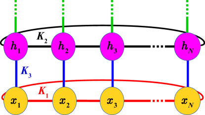
Figure 1: (color online). Structure of the unrestricted Boltzmann machine. The lower (yellow) nodes depict visible spins, the upper (magenta) nodes depict the hidden spins. The horizontal segments indicate intralayer visible-visible and hidden-hidden correlations. The vertical (blue) segments represent the interlayer correlations between the corresponding visible and hidden spins. The green lines allude to a possible extension to deep layers architectures.

In the case of an uRBM variational wave function, the average value of the energy $E={\langle\hat{H}\rangle}$ is computed as follows

$${\langle\hat{H}\rangle} = \frac{\langle\Psi_{\boldsymbol{\kappa}}|\hat{H}|\Psi_{\boldsymbol{\kappa}}\rangle}{\langle\Psi_{\boldsymbol{\kappa}}|\Psi_{\boldsymbol{\kappa}}\rangle}=\frac{\sum_{\mathit{\boldsymbol{x}},\mathit{\boldsymbol{x}}^{\prime}}\Psi_{\boldsymbol{\kappa}}(\mathit{\boldsymbol{x}})H_{\mathit{\boldsymbol{x}},\mathit{\boldsymbol{x}}^{\prime}}\Psi_{\boldsymbol{\kappa}}(\mathit{\boldsymbol{x}}^{\prime})}{\sum_{\mathit{\boldsymbol{x}}}\Psi_{\boldsymbol{\kappa}}(\mathit{\boldsymbol{x}})\Psi_{\boldsymbol{\kappa}}(\mathit{\boldsymbol{x}})}$$ (5)

$$= \frac{\sum_{\mathit{\boldsymbol{x}},\mathit{\boldsymbol{x}}^{\prime}}\left[\sum_{\mathit{\boldsymbol{h}}_{\bf a}}\phi_{\boldsymbol{\kappa}}(\mathit{\boldsymbol{x}},\mathit{\boldsymbol{h}}_{\bf a})\right]H_{\mathit{\boldsymbol{x}},\mathit{\boldsymbol{x}}^{\prime}}\left[\sum_{\mathit{\boldsymbol{h}}_{\bf b}}\phi_{\boldsymbol{\kappa}}(\mathit{\boldsymbol{x}}^{\prime},\mathit{\boldsymbol{h}}_{\bf b})\right]}{\sum_{\mathit{\boldsymbol{x}}}\left[\sum_{\mathit{\boldsymbol{h}}_{\bf a}}\phi_{\boldsymbol{\kappa}}(\mathit{\boldsymbol{x}},\mathit{\boldsymbol{h}}_{\bf a})\right]\left[\sum_{\mathit{\boldsymbol{h}}_{\bf b}}\phi_{\boldsymbol{\kappa}}(\mathit{\boldsymbol{x}},\mathit{\boldsymbol{h}}_{\bf b})\right]}$$

$$= \ll E_{\mathrm{loc}}(\mathit{\boldsymbol{x}},\mathit{\boldsymbol{h}}_{\bf b})\gg\;,$$

where the local energy $E_{\mathrm{loc}}(\mathit{\boldsymbol{x}},\mathit{\boldsymbol{h}})$ is defined as

$$E_{\mathrm{loc}}(\mathit{\boldsymbol{x}},\mathit{\boldsymbol{h}})=\frac{\sum_{\mathit{\boldsymbol{x}}^{\prime}}H_{\mathit{\boldsymbol{x}},\mathit{\boldsymbol{x}}^{\prime}}\phi_{\boldsymbol{\kappa}}(\mathit{\boldsymbol{x}}^{\prime},\mathit{\boldsymbol{h}})}{\phi_{\boldsymbol{\kappa}}(\mathit{\boldsymbol{x}},\mathit{\boldsymbol{h}})}\;,$$ (6)

with $H_{\mathit{\boldsymbol{x}},\mathit{\boldsymbol{x}}^{\prime}}=\langle\mathit{\boldsymbol{x}}|\hat{H}|\mathit{\boldsymbol{x}}^{\prime}\rangle$. $\mathit{\boldsymbol{h}}_{\bf a}$ and $\mathit{\boldsymbol{h}}_{\bf b}$ indicate two hidden spin configurations. Notice that the formula for the local energy can be symmetrized with respect to the two sets of hidden spins $\mathit{\boldsymbol{h}}_{\bf a}$ and $\mathit{\boldsymbol{h}}_{\bf b}$, providing results with slightly reduced statistical fluctuations. The double brackets $\ll\cdots\gg$ indicate the expectation value over the visible-spin configurations $\mathit{\boldsymbol{x}}$ and two sets of hidden spins configurations $\mathit{\boldsymbol{h}}_{\bf a}$ and $\mathit{\boldsymbol{h}}_{\bf b}$, sampled from the following normalized probability distribution:

$$p(\mathit{\boldsymbol{x}},\mathit{\boldsymbol{h}}_{\bf a},\mathit{\boldsymbol{h}}_{\bf b})=\frac{\phi_{\boldsymbol{\kappa}}(\mathit{\boldsymbol{x}},\mathit{\boldsymbol{h}}_{\bf a})\phi_{\boldsymbol{\kappa}}(\mathit{\boldsymbol{x}},\mathit{\boldsymbol{h}}_{\bf b})}{\sum_{\mathit{\boldsymbol{x}},\mathit{\boldsymbol{h}}_{\bf a},\mathit{\boldsymbol{h}}_{\bf b}}\phi_{\boldsymbol{\kappa}}(\mathit{\boldsymbol{x}},\mathit{\boldsymbol{h}}_{\bf a})\phi_{\boldsymbol{\kappa}}(\mathit{\boldsymbol{x}},\mathit{\boldsymbol{h}}_{\bf b})}\;.$$ (7)

As in standard Monte Carlo approaches, this expectation value is estimated as the average of $E_{\mathrm{loc}}(\mathit{\boldsymbol{x}},\mathit{\boldsymbol{h}})$ over a (large) set of uncorrelated configurations, sampled according to $p(\mathit{\boldsymbol{x}},\mathit{\boldsymbol{h}}_{\bf a},\mathit{\boldsymbol{h}}_{\bf b})$. The statistical uncertainty can be reduced at will by increasing the number of sampled configurations. The optimal variational parameters $\boldsymbol{\kappa}_{\mathrm{opt}}$ that minimize the energy expectation value can be found using a stochastic optimization method. We adopt a relatively simple yet quite efficient one, namely the stochastic gradient descent algorithm (see, e.g., Becca and Sorella (2017)). While more sophisticated algorithms exist as, e.g., the stochastic reconfiguration method Sorella et al. (2007), such methods are not necessary here since the Ansätze that we consider include a very small number of variational parameters, one or three. In fact, in these cases the optimal variational parameters can be obtained also by performing a scan on a fine grid. By doing so, we obtain essentially the same results provided by the stochastic gradient descent algorithm.

We assess the accuracy of the optimized variational wave functions by calculating the relative error

$$e_{\mathrm{rel}}=\frac{\left|E-E_{\mathrm{JW}}\right|}{\left|E_{\mathrm{JW}}\right|}\;,$$ (8)

in the obtained variational estimate $E$ of the ground state energy of the Hamiltonian in Eq. (1). $E_{\mathrm{JW}}$ is the exact finite size ground state energy of the quantum Ising chain. It is obtained by performing the Jordan–Wigner transformation, followed by a Fourier and the Bogoliubov transformations.

Figure 2 displays the relative error $e_{\mathrm{rel}}$ in Eq. (8) corresponding to the variational wave functions introduced above, as a function of the transverse field $\Gamma$. The system size is $N=80$, which is here representative of the thermodynamic limit. The Boltzmann-type Ansatz does not provide particularly accurate predictions. In the ferromagnetic phase $\Gamma<1$, the relative error is up to $10\%$. The uRBM, instead, provides very accurate predictions. The relative error is always below $0.1\%$. The largest discrepancy occurs at the quantum critical point $\Gamma=1$. Such high accuracy is remarkable, considering that the uRBM Ansatz involves only $3$ variational parameters. It is also worth mentioning that very similar accuracies are obtained also for different system sizes. Therefore, the uRBM Ansatz represents a promising guiding function for simulations of quantum annealing optimization of disordered models. As a term of comparison, we show in Fig. 2 the results obtained in Ref. Carleo and Troyer, 2017 using the RBM Ansatz. The relative errors corresponding to the RBM with hidden-unit density $\alpha=1$ are larger than those corresponding to the uRBM, despite the fact that the RBM Ansatz involves a larger number of variational parameters. However, it is worth stressing that the RBM results can be systematically improved by increasing $\alpha$. For example, with $\alpha=2$ the RBM relative errors are approximately an order of magnitude smaller than those corresponding to the uRBM Ansatz.

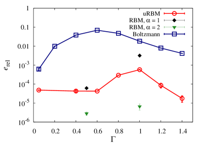
Figure 2: (color online). Relative error $e_{\mathrm{rel}}$ in the variational estimates of the ground-state energy, see Eq. (8), as a function of the transverse field $\Gamma$, obtained using the simple Boltzmann wave function and for the unrestricted Boltzmann machine (uRBM) Ansatz. The system size is $N=80$. For comparison, we also show the data corresponding to the restricted Boltzmann machine (RBM) from Ref. Carleo and Troyer, 2017, where $\alpha$ indicates the hidden-spin density. The thin lines are guides to the eyes.

III Importance sampling guided by unrestricted neural network states

In this section we discuss how optimized variational wave functions can be utilized to boost the performance of PQMC simulations. First, we consider the implementation of the PQMC algorithm without guiding functions. PQMC methods allow one to extract ground-state properties of quantum many-body systems Anderson (1975); Kalos and Whitlock (2008) by stochastically simulating the Schrödinger equation in imaginary-time $\tau=it$. In the Dirac notation, this equation is written as:

$$-\frac{\partial}{\partial\tau}|\Psi(\tau)\rangle=(\hat{H}-E_{\mathrm{ref}})|\Psi(\tau)\rangle.$$ (9)

The reduced Planck constant is set to $\hbar=1$ throughout this Article. $E_{\mathrm{ref}}$ is a reference energy introduced to stabilize the simulation, as discussed later. Eq. (9) is simulated by iteratively applying the equation $\Psi(\mathit{\boldsymbol{x}},\tau+\Delta\tau)=\sum_{\mathit{\boldsymbol{x}}^{\prime}}G(\mathit{\boldsymbol{x}},\mathit{\boldsymbol{x}}^{\prime},\Delta\tau)\Psi(\mathit{\boldsymbol{x}}^{\prime},\tau)$. $\Delta\tau$ is a (short) time step and $G({\mathit{\boldsymbol{x}}},{\mathit{\boldsymbol{x}}}^{\prime},\Delta\tau)=\langle\mathit{\boldsymbol{x}}|e^{-\Delta\tau(\hat{H}-E_{\mathrm{ref}})}|\mathit{\boldsymbol{x}}^{\prime}\rangle$ is the Green’s function of Eq. (9). Below it is discussed how one can write a suitable explicit expression. Long propagation times $\tau$ are achieved by iterating many (small) time steps $\Delta\tau$, allowing one to sample, in the $\tau\rightarrow\infty$ limit, spin configurations with a probability density proportional to the ground state wave function $\Psi_{0}(\mathit{\boldsymbol{x}})$ (assumed to be real and non negative). One should notice that the Green’s function $G({\mathit{\boldsymbol{x}}},{\mathit{\boldsymbol{x}}}^{\prime},\Delta\tau)$ does not define a stochastic matrix; while its elements are nonnegative, one has $\sum_{\mathit{\boldsymbol{x}}}G({\mathit{\boldsymbol{x}}},{\mathit{\boldsymbol{x}}}^{\prime},\Delta\tau)\neq 1$, in general. Therefore, it cannot be utilized to define the transition matrix of a conventional Markov chain Monte Carlo simulation. This problem can be circumvented by rewriting the Green’s function as $G({\mathit{\boldsymbol{x}}},{\mathit{\boldsymbol{x}}}^{\prime},\Delta\tau)=G_{\mathrm{T}}({\mathit{\boldsymbol{x}}},{\mathit{\boldsymbol{x}}}^{\prime},\Delta\tau)b_{\mathit{\boldsymbol{x}}^{\prime}}$, where $G_{\mathrm{T}}({\mathit{\boldsymbol{x}}},{\mathit{\boldsymbol{x}}}^{\prime},\Delta\tau)$ is by definition stochastic, and the normalization factor is $b_{\mathit{\boldsymbol{x}}^{\prime}}=\sum_{\mathit{\boldsymbol{x}}}G({\mathit{\boldsymbol{x}}},{\mathit{\boldsymbol{x}}}^{\prime},\Delta\tau)$. A stochastic process can then be implemented, where a large population of equivalent copies of the system, in jargon called walkers, is evolved. Each walker represents one possible spin configuration ${\mathit{\boldsymbol{x}}}_{n}^{\prime}$ (the index $n$ labels different walkers), and is gradually modified by performing spin-configuration updates according to $G_{\mathrm{T}}({\mathit{\boldsymbol{x}}}_{n},{\mathit{\boldsymbol{x}}}_{n}^{\prime},\Delta\tau)$. Thereafter, their (relative) weights $w_{n}$ are accumulated according to the rule $w_{n}\rightarrow w_{n}b_{\mathit{\boldsymbol{x}}_{n}^{\prime}}$, starting with equal initial weights $w_{n}=1$ for all the walkers in the initial population. While this implementation is in principle correct, it is known to lead to an exponentially fast signal loss as the number of Monte Carlo steps increases. This is due to the fact that the relative weight of few walkers quickly becomes dominant, while most other walkers give a negligible contribution to the signal. An effective remedy consists in introducing a branching process, where each walker is replicated (or annihilated) a number of times corresponding, on average, to the weight $w_{n}$. The simplest correct rule consists in generating, for each walker in the population at a certain imaginary time $\tau$, a number of descendants $n_{\mathrm{d}}$ in the population at imaginary time $\tau+\Delta\tau$. $n_{\mathrm{d}}$ is defined as $\mathrm{int}\left[w_{n}+\eta\right]$, where $\eta\in\left[0,1\right]$ is a uniform random number, and the function $\mathrm{int}\left[\right]$ gives the integer part of the argument Thijssen (2007). Clearly, after branching has been performed, all walkers have the same weight $w_{n}=1$. Therefore, the number of walkers in the population fluctuates at each PQMC iteration and can be kept close to a target value by adjusting the reference energy $E_{\mathrm{ref}}$. Introducing the branching process provides one with a feasible, possibly efficient algorithm. However, such as process might actually introduce a systematic bias if the average population size $N_{w}$ is not large enough. The bias originates from the spurious correlations among walkers generated from the same ancestor Becca and Sorella (2017). This effect becomes negligible in the $N_{w}\rightarrow\infty$ limit, but might be sizable for finite $N_{w}$. It is known to be the most relevant and subtle possible source of systematic errors in PQMC algorithms Nemec (2010); Boninsegni and Moroni (2012); Pollet et al. (2018). In fact, it was shown in Ref. Inack et al. (2018) that in order to determine with a fixed target relative error, the ground state energy of the ferromagnetic quantum Ising chain with the (simple) diffusion Monte Carlo algorithm (which belongs to the category of PQMC methods), the walker-population size $N_{w}$ has to exponentially increase with the system size $N$. This implies an exponentially scaling computational cost.

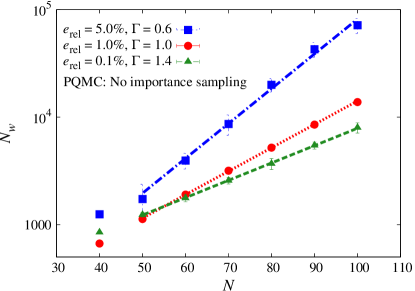
Figure 3: (color online). Number of random walkers $N_{w}$ required to determine, using the PQMC algorithm without importance sampling, the ground-state energy with a relative error $e_{\mathrm{rel}}$, see Eq. (8), as a function of the system size $N$. Different datasets correspond to different transverse field intensities $\Gamma$ and different relative errors. The lines represent exponential fitting functions.

A promising strategy to circumvent the aforementioned problem is to introduce the so-called importance sampling technique. This is indeed a well established approach to boost the efficiency of PQMC simulations (see, e.g, Ref. Foulkes et al. (2001)) because it has the potential to reduce the number of walkers needed to attain a given accuracy Becca and Sorella (2017). It consists in evolving a function $f({\mathit{\boldsymbol{x}}},\tau)=\Psi({\mathit{\boldsymbol{x}}},\tau)\psi_{T}({\mathit{\boldsymbol{x}}})$ via a modified imaginary-time Schrödinger equation. $\psi_{T}({\mathit{\boldsymbol{x}}})$ is a guiding function designed to accurately approximate the ground-state wave function. Its role is to favor the sampling of configurations with high probability amplitude. The obtained modified imaginary-time Schrödinger equation is solved via a Markov process defined by the following equation:

$$f(\mathit{\boldsymbol{x}},\tau+\Delta\tau)=\sum_{\mathit{\boldsymbol{x}}^{\prime}}\tilde{G}(\mathit{\boldsymbol{x}},\mathit{\boldsymbol{x}}^{\prime},\Delta\tau)f(\mathit{\boldsymbol{x}}^{\prime},\tau),$$ (10)

where the modified Green’s function is given by $\tilde{G}({\mathit{\boldsymbol{x}}},{\mathit{\boldsymbol{x}}}^{\prime},\Delta\tau)=G(\mathit{\boldsymbol{x}},\mathit{\boldsymbol{x}}^{\prime},\Delta\tau)\frac{\psi_{T}({\mathit{\boldsymbol{x}}})}{\psi_{T}({\mathit{\boldsymbol{x}}^{\prime}})}$. A suitable approximation for the modified Green’s function can be obtained by dividing the time step $\Delta\tau$ into $M$ shorter time steps $\delta\tau=\Delta\tau/M$. If $\delta\tau$ is sufficiently short, one can employ a Taylor expansion truncated at the linear term, $\tilde{G}({\mathit{\boldsymbol{x}}},{\mathit{\boldsymbol{x}}}^{\prime},\Delta\tau)\cong\left[\tilde{g}({\mathit{\boldsymbol{x}}},{\mathit{\boldsymbol{x}}}^{\prime},\delta\tau)\right]^{M}$, where:

$$\tilde{g}({\mathit{\boldsymbol{x}}},{\mathit{\boldsymbol{x}}}^{\prime},\delta\tau)=\big{[}\delta_{\mathit{\boldsymbol{x}},\mathit{\boldsymbol{x}}^{\prime}}-\delta\tau(H_{\mathit{\boldsymbol{x}},\mathit{\boldsymbol{x}}^{\prime}}-E_{\mathrm{ref}}\delta_{\mathit{\boldsymbol{x}},\mathit{\boldsymbol{x}}^{\prime}})\big{]}\frac{\psi_{T}({\mathit{\boldsymbol{x}}})}{\psi_{T}({\mathit{\boldsymbol{x}}^{\prime}})}\;.$$ (11)

With this approximation, Eq. (10) defines a stochastic implementation of the power method of linear algebra. Convergence to the exact ground state is guaranteed as long as $\delta\tau$ is smaller than a finite value, sufficiently small to ensure that all matrix elements of $\tilde{g}({\mathit{\boldsymbol{x}}},{\mathit{\boldsymbol{x}}}^{\prime},\delta\tau)$ are not negative Schmidt et al. (2005). As the system size increases, shorter and shorter time steps $\delta\tau$ are required. This leads to pathologically inefficient simulations, since in this regime the identity operator dominates, resulting in extremely long autocorrelation times. This problem can be solved by adopting the continuous-time Green’s function Monte Carlo (CTGFMC) algorithm. The derivation and the details of this algorithm are given in Ref. Becca and Sorella (2017); Sorella and Capriotti (2000), and so we only sketch it here. The idea is to formally take the $M\rightarrow\infty$ limit, and determine the (stochastic) time interval $\delta\tau^{\prime}$ that passes before the next configuration update occurs. It is convenient to bookkeep the remaining time $\delta\tau_{t}$ left to complete a total interval of time $\Delta\tau$. This is to ensure that each iteration of the PQMC simulation corresponds to a time step of duration $\Delta\tau$. The time interval $\delta\tau^{\prime}$ is sampled using the formula $\delta\tau^{\prime}=\mathrm{Min}\big{(}\delta\tau_{t},\frac{\ln(1-\xi)}{E_{\mathrm{loc}}(\mathit{\boldsymbol{x}}^{\prime})-E_{\mathrm{cl}}(\mathit{\boldsymbol{x}}^{\prime})}\big{)}$ with $\xi\in(0,1)$ being a uniform random number. The spin-configuration update $\mathit{\boldsymbol{x}}^{\prime}\rightarrow\mathit{\boldsymbol{x}}$ (with $\mathit{\boldsymbol{x}}^{\prime}\neq\mathit{\boldsymbol{x}}$) is randomly selected from the probability distribution

$$\begin{array}[]{ll}t_{{\mathit{\boldsymbol{x}}},{\mathit{\boldsymbol{x}}}^{\prime}}&=\displaystyle\frac{p_{{\mathit{\boldsymbol{x}}},{\mathit{\boldsymbol{x}}}^{\prime}}}{\sum_{\mathit{\boldsymbol{x}}\neq\mathit{\boldsymbol{x}}^{\prime}}p_{{\mathit{\boldsymbol{x}}},{\mathit{\boldsymbol{x}}}^{\prime}}}\vspace{2mm}\\ p_{{\mathit{\boldsymbol{x}}},{\mathit{\boldsymbol{x}}}^{\prime}}&=\displaystyle\frac{\tilde{g}({\mathit{\boldsymbol{x}}},{\mathit{\boldsymbol{x}}}^{\prime},\delta\tau^{\prime})}{\sum_{\mathit{\boldsymbol{x}}}\tilde{g}({\mathit{\boldsymbol{x}}},{\mathit{\boldsymbol{x}}}^{\prime},\delta\tau^{\prime})}\end{array}\;.$$ (12)

Notice that, with the Hamiltonian (1), $\mathit{\boldsymbol{x}}$ differs from $\mathit{\boldsymbol{x}}^{\prime}$ only for one spin flip. The weight-update factor for the branching process takes the exponential form $b_{\mathit{\boldsymbol{x}}^{\prime}}=e^{-\delta\tau^{\prime}[E_{\mathrm{loc}}(\mathit{\boldsymbol{x}}^{\prime})-E_{\mathrm{ref}}]}$, where the local energy is now $E_{\mathrm{loc}}(\mathit{\boldsymbol{x}}^{\prime})=\sum_{\mathit{\boldsymbol{x}}}H_{\mathit{\boldsymbol{x}},\mathit{\boldsymbol{x}}^{\prime}}\frac{\psi_{T}({\mathit{\boldsymbol{x}}})}{\psi_{T}({\mathit{\boldsymbol{x}}^{\prime}})}$.

In summary, the CTGFMC algorithm requires to perform, for each walker $n$ in the population, the following steps:

i)

initialize the time interval $\delta\tau_{t}=\Delta\tau$, and the weight factor $w_{n}=1$;

ii)

sample the time $\delta\tau^{\prime}$ at which the the configuration update $\mathit{\boldsymbol{x}}^{\prime}\rightarrow\mathit{\boldsymbol{x}}$ might occur;

iii)

if $\delta\tau^{\prime}<\delta\tau_{t}$, update $\mathit{\boldsymbol{x}}^{\prime}$ with a transition probability $t_{{\mathit{\boldsymbol{x}}},{\mathit{\boldsymbol{x}}}^{\prime}}$ in Eq. (12), else set $\delta\tau^{\prime}=\delta\tau_{t}$;

iv)

accumulate the weight factor according to the rule $w_{n}\rightarrow w_{n}b_{\mathit{\boldsymbol{x}}^{\prime}}$ and set $\delta\tau_{t}\rightarrow\delta\tau_{t}-\delta\tau^{\prime}$;

v)

Go back to step ii) until $\delta\tau_{t}=0$;

vi)

finally, perform branching according to the total accumulated weight factor $w_{n}$.

This continuous-time algorithm implicitly implements the exact imaginary-time modified Green’s function $\tilde{G}({\mathit{\boldsymbol{x}}},{\mathit{\boldsymbol{x}}}^{\prime},\Delta\tau)$.

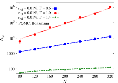
Figure 4: (color online). Number of random walkers $N_{w}$ required to determine, using the optimized Boltzmann-type wave function to guide importance sampling in the PQMC simulation, the ground-state energy with a relative error $e_{\mathrm{rel}}$, see Eq. (8), as a function of the system size $N$. Different datasets correspond to different transverse field intensities $\Gamma$. The (red) dotted and (blue) dot-dashed lines represent exponential fitting functions, while the (green) dashed line represents a power-law fit with power $b=0.54(5)$.

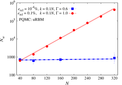
Figure 5: (color online). Number of random walkers $N_{w}$ required to determine, using the optimized uRBM Ansatz to guide importance sampling in the PQMC simulation, the ground-state energy with a relative error $e_{\mathrm{rel}}$, see Eq. (8), as a function of the system size $N$. The number of single-spin Metropolis updates of the hidden spins per CTGFMC hidden-spin update is $k=0.1N$. The (red) dotted line represents and exponential fit, while the (blue) dot-dashed line represents a linear fit.

In the long imaginary-time limit, the walkers sample spin configurations with a probability distribution proportional to $f(\mathit{\boldsymbol{x}},\tau\rightarrow\infty)=\Psi_{0}({\mathit{\boldsymbol{x}}})\psi_{T}({\mathit{\boldsymbol{x}}})$. If $\psi_{T}({\mathit{\boldsymbol{x}}})$ is a good approximation of the ground-state wave function, this distribution closely approximates the quantum-mechanical probability of finding the system in the spin configuration $\mathit{\boldsymbol{x}}$. It is important to notice that if our guiding wave function was exact, i.e. if $\psi_{T}({\mathit{\boldsymbol{x}}})=\Psi_{0}({\mathit{\boldsymbol{x}}})$, then the local energy $E_{\mathrm{loc}}(\mathit{\boldsymbol{x}})$ would be a constant function. This would completely suppress the fluctuations of the number of walkers, therefore eliminating the bias due to the finite walkers population $N_{w}$. If $\psi_{T}({\mathit{\boldsymbol{x}}})$ is, albeit not exact, a good approximation of $\Psi_{0}({\mathit{\boldsymbol{x}}})$, the fluctuations of the number of walkers are still reduced compared to the case of the simple CTGFMC algorithm (which corresponds to setting $\psi_{T}(\mathit{\boldsymbol{x}})=1$) giving a faster convergence to the exact $N_{w}\rightarrow\infty$ limit. Below we consider the use of the variational wave-functions $\Psi_{\boldsymbol{\kappa}}(\mathit{\boldsymbol{x}})$ described in Sec. II as guiding wave-functions for the PQMC algorithm, setting the variational parameters $\boldsymbol{\kappa}$ at their optimal values.

In order to employ the unrestricted neural-network states as guiding functions, the PQMC algorithm has to be modified. One has to implement a combined dynamics of the visible-spin configurations $\mathit{\boldsymbol{x}}$ and of the hidden-spin configurations $\mathit{\boldsymbol{h}}$. We will indicate the global configuration as $\mathit{\boldsymbol{y}}=(\mathit{\boldsymbol{x}},\mathit{\boldsymbol{h}})$. The goal is to sample global configurations with the (normalized) probability distribution

$$p(\mathit{\boldsymbol{y}})=\frac{\Psi_{0}(\mathit{\boldsymbol{x}})\phi_{\boldsymbol{\kappa}}(\mathit{\boldsymbol{x}},\mathit{\boldsymbol{h}})}{\sum_{\mathit{\boldsymbol{x}},\mathit{\boldsymbol{h}}}\Psi_{0}(\mathit{\boldsymbol{x}})\phi_{\boldsymbol{\kappa}}(\mathit{\boldsymbol{x}},\mathit{\boldsymbol{h}})}\;.$$ (13)

This allows one to compute the ground state energy as $E=\lim_{N_{c}\rightarrow\infty}\sum_{i=1}^{N_{c}}E_{\mathrm{loc}}(\mathit{\boldsymbol{x}}_{i},\mathit{\boldsymbol{h}}_{i})/N_{c}$, where $N_{c}$ is a number of uncorrelated configurations $\left\{\mathit{\boldsymbol{y}}_{i}\right\}$ sampled from $p(\mathit{\boldsymbol{y}})$. The local energy $E_{\mathrm{loc}}(\mathit{\boldsymbol{x}},\mathit{\boldsymbol{h}})$ is defined as in Eq. (6). A suitable algorithm was implemented in Ref. Vitiello and Whitlock (1991) in the case of the continuous-space Green’s function Monte Carlo algorithm, where importance sampling was implemented using shadow wave functions. Here we modify the approach of Ref. Vitiello and Whitlock (1991) to address quantum spin models. The visible-spins configurations $\mathit{\boldsymbol{x}}$ are evolved according to the CTGFMC described above, keeping the hidden-spin configuration $\mathit{\boldsymbol{h}}^{\prime}$ fixed. The modified imaginary-time Green’s function is now $\tilde{G}({\mathit{\boldsymbol{x}}},{\mathit{\boldsymbol{x}}}^{\prime},\Delta\tau|\mathit{\boldsymbol{h}}^{\prime})=G(\mathit{\boldsymbol{x}},\mathit{\boldsymbol{x}}^{\prime},\Delta\tau)\frac{\phi_{\boldsymbol{\kappa}}(\mathit{\boldsymbol{x}},\mathit{\boldsymbol{h}}^{\prime})}{\phi_{\boldsymbol{\kappa}}(\mathit{\boldsymbol{x}}^{\prime},\mathit{\boldsymbol{h}}^{\prime})}$. As discussed above, this has to be rewritten as the product of a stochastic matrix, which defines how the visible-spin configurations updates are selected, and a weight term, which is taken into account with the branching process. The weight-update factor is $b_{\mathit{\boldsymbol{y}}^{\prime}}=\sum_{\mathit{\boldsymbol{x}}}\tilde{G}({\mathit{\boldsymbol{x}}},{\mathit{\boldsymbol{x}}}^{\prime},\Delta\tau|\mathit{\boldsymbol{h}}^{\prime})$. The dynamics of the hidden-spins configurations is dictated by a (classical) Markov chain Monte Carlo algorithm. Considering $\phi_{\boldsymbol{\kappa}}(\mathit{\boldsymbol{x}},\mathit{\boldsymbol{h}})$ as an unnormalized probability distribution allows one to write — for any fixed visible-spin configuration $\mathit{\boldsymbol{x}}$ — the Master equation:

$$\phi_{\boldsymbol{\kappa}}(\mathit{\boldsymbol{x}},\mathit{\boldsymbol{h}})=\sum_{\mathit{\boldsymbol{h}}^{\prime}}T(\mathit{\boldsymbol{h}},\mathit{\boldsymbol{h}}^{\prime}|\mathit{\boldsymbol{x}})\phi_{\boldsymbol{\kappa}}(\mathit{\boldsymbol{x}},\mathit{\boldsymbol{h}}^{\prime}),$$ (14)

where $T(\mathit{\boldsymbol{h}},\mathit{\boldsymbol{h}}^{\prime}|\mathit{\boldsymbol{x}})$ is the transition matrix that defines the Markov process. Clearly, the following condition must be fulfilled $\sum_{\mathit{\boldsymbol{h}}}T(\mathit{\boldsymbol{h}},\mathit{\boldsymbol{h}}^{\prime}|\mathit{\boldsymbol{x}})=1$, for any $\mathit{\boldsymbol{x}}$.

Our choice is a single spin flip Metropolis algorithm, where the flip of a randomly selected spin is proposed, and accepted with the probability

$$A(\mathit{\boldsymbol{h}}^{\prime}\rightarrow\mathit{\boldsymbol{h}}|\mathit{\boldsymbol{x}})=\mathrm{Min}\left\{1,\frac{\phi_{\boldsymbol{\kappa}}(\mathit{\boldsymbol{x}},\mathit{\boldsymbol{h}})}{\phi_{\boldsymbol{\kappa}}(\mathit{\boldsymbol{x}},\mathit{\boldsymbol{h}}^{\prime})}\right\}.$$ (15)

Here, $\mathit{\boldsymbol{h}}$ differs from $\mathit{\boldsymbol{h}}^{\prime}$ only for the (randomly selected) flipped spin. One could perform a certain number, call it $k$, of Metropolis updates, without modifying the formalism. In fact, this turns out to be useful, as discussed below. The combined dynamics of the visible and the hidden spins is driven by the following equation:

$$f(\mathit{\boldsymbol{y}},\tau+\Delta\tau)=\sum_{\mathit{\boldsymbol{y}}^{\prime}}G(\mathit{\boldsymbol{y}},\mathit{\boldsymbol{y}}^{\prime},\Delta\tau)f(\mathit{\boldsymbol{y}}^{\prime},\tau),$$ (16)

with $G(\mathit{\boldsymbol{y}},\mathit{\boldsymbol{y}}^{\prime},\Delta\tau)=T(\mathit{\boldsymbol{h}},\mathit{\boldsymbol{h}}^{\prime}|\mathit{\boldsymbol{x}})\tilde{G}({\mathit{\boldsymbol{x}}},{\mathit{\boldsymbol{x}}}^{\prime},\Delta\tau|\mathit{\boldsymbol{h}}^{\prime})$. It can be shown Vitiello and Whitlock (1991) that the equilibrium probability distribution of this equation is the desired joint probability distribution $p(\mathit{\boldsymbol{y}})$ in Eq. (13). The stochastic process corresponding to this equation can be implemented with the following steps:

i)

perform the visible-spin configuration update $\mathit{\boldsymbol{x}}^{\prime}\rightarrow\mathit{\boldsymbol{x}}$, keeping $\mathit{\boldsymbol{h}}^{\prime}$ fixed, according to the CTGFMC algorithm described above (including accumulation of the weight factor);

ii)

perform $k$ single-spin Metropolis updates of the hidden-spin configuration $\mathit{\boldsymbol{h}}^{\prime}$, keeping $\mathit{\boldsymbol{x}}$ fixed;

iii)

perform branching of the global configuration.

It is easily shown that the hidden-spin dynamics does not directly affect the weight factor since the normalization of the Green function of the combined dynamics is set by $b_{\mathit{\boldsymbol{y}}^{\prime}}$.

Since the optimized uRBM describes the ground state wave function with high accuracy, one expects that its use as guiding function leads to a drastic reduction of the systematic errors due to the finite random walker population. However, one should take into account that there might be statistical correlations among subsequent hidden-spin configurations along the Markov chain. This might in turn affect the systematic error. Clearly, increasing the number of Metropolis steps $k$ per CTGFMC visible-spin configuration update allows one to suppress such correlations, possibly reducing the systematic error. This will indeed turn out to be important, in particular at the quantum critical point where statistical correlations along the Markov chain are more significant.

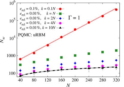
Figure 6: (color online). Number of random walkers $N_{w}$ required to determine, using the optimized uRBM to guide importance sampling in the PQMC simulation, the ground-state energy with a relative error $e_{\mathrm{rel}}$, see Eq. (8), as a function of the system size $N$. The transverse field intensity is set at the ferromagnetic quantum critical point $\Gamma=1$. Different datasets correspond to different values of the the number of single-spin Metropolis updates $k$. The (red) dotted line represents an exponential fit, while the (black) dot-dashed line represents a power-law fit, with power $b=0.55(1)$.

Following Ref. Inack et al., 2018, we analyze the computational complexity of the PQMC algorithm by determining the number of walkers $N_{w}$ needed to determine the ground state energy of the Hamiltonian (1) with a prescribed accuracy. All data described below have been obtained with a time step $\Delta\tau=0.1$, and all simulations have been run for a long enough total imaginary time to ensure equilibration.

First, we consider the simple PQMC algorithm i.e., performed without importance sampling. Fig. 3 displays the scaling with the system size $N$ of the number of walkers $N_{w}$ required to keep the relative error $e_{\mathrm{rel}}$, defined in Eq. (8), at the chosen threshold. This scaling is evidently exponential, below, above, and also at the quantum critical point. The most severe scaling comes from the ordered phase and could be attributed to the fact that the simple PQMC is formally equivalent to PQMC with a constant $\psi_{T}(\mathit{\boldsymbol{x}})$ for importance sampling. This turns out to be a very poor choice of the guiding function in the ordered regime given that it treats all configurations on an equal footing. Analogous results have been obtained in Ref. Inack et al., 2018 using the diffusion Monte Carlo algorithm. This is another PQMC method — in fact very similar to the CTGFMC algorithm employed here — whose transition matrix is defined from the imaginary time Green’s function derived within the symmetrized Trotter decomposition. Introducing importance sampling using the optimized Boltzmann-type Ansatz as guiding function significantly reduces the systematic error due to the finite random walker population, allowing one to reach quite small relative errors. In particular, in the paramagnetic phase at $\Gamma=1.4$, the scaling of $N_{w}$ versus $N$ is quite flat (see Fig. 4); it appears to be well described by the power-law $N_{w}\sim N^{b}$ with the small power $b=0.54(5)$, rather than by an exponential. However, in the ferromagnetic phase at $\Gamma=0.6$ and at the quantum critical point $\Gamma=1$ the scaling is still clearly exponential. This means that the simple Boltzmann-type Ansatz is, in general, insufficient to ameliorate the exponentially scaling computational cost of the PQMC algorithm. Fig. 5 shows the scaling of $N_{w}$ obtained using the optimized uRBM Ansatz as the guiding function. The number of hidden-spin Metropolis steps per visible-spin update is set to a (small) fraction of the system size $N$, namely to $k=0.1N$. At $\Gamma=0.6$, the required walker population size $N_{w}$ turns out to be essentially independent on the system size $N$. It is worth noticing that the prescribed relative error is here as small as $e_{\mathrm{rel}}=10^{-6}$, and that this high accuracy is achieved with a rather small walkers population $N_{w}\lesssim 1000$. However, at the quantum critical point, $N_{w}$ still displays an exponential scaling with system size. This effect can be traced back to the diverging statistical correlations among subsequent hidden-spin configurations along the Markov chain, due to quantum criticality. As anticipated above, these statistical correlations can be suppressed by increasing the number of hidden-spin updates $k$. Fig. 6 displays the scaling of $N_{w}$, at the quantum critical point, for different $k$ values. One observes that the scaling substantially improves already for moderately larger $k$ values, leading to a crossover from the exponential scaling obtained with $k=0.1N$, to a square-root like scaling $N_{w}\sim N^{0.55(1)}$ when $k=10N$. It is important to point out that increasing $k$ implies a correspondingly increasing contribution to the global computational cost of the PQMC algorithm. However, since $k$ is here linear in the system size, this contribution does not modify, to leading order, the scaling of the global computational cost. Therefore, one can conclude that the uRBM Ansatz is sufficient to change the scaling of the computational cost of the PQMC algorithm from exponential in the system size, to an amenable polynomial scaling. In the simulations presented here, single-spin flip Metropolis updates are employed for the hidden variables. It is possible that cluster spin updates would lead to an even faster convergence to the exact $N_{w}\rightarrow\infty$ limit, due to the more efficient sampling of the hidden-spin configurations. However, such cluster updates cannot always be implemented, in particular for frustrated disordered Hamiltonians relevant for optimization problems; therefore, we do not consider them here.

IV Conclusions

The accuracy of variational wave-functions that mimic unrestricted Boltzmann machines, which we refer to as unrestricted neural network states, has been analyzed using the one-dimensional ferromagnetic Ising model as a testbed. By optimizing just three variational parameters, ground-state energies with a relative error smaller than $10^{-3}$ have been obtained. The ferromagnetic quantum phase transition turns out to be the point where the relative error is the largest. This accuracy is comparable to the one previously obtained using restricted neural network states with few hidden variables per visible spin Carleo and Troyer (2017). These restricted neural network states involve a number of variational parameters proportional to the system size, as opposed to the unrestricted neural network states considered here, where the (small) number of variational parameters is fixed. This feature of the unrestricted states makes them very suitable in the context of quantum annealing simulations for Ising-type models (which are sign-problem free). However, since one has to integrate over hidden-spins configurations via Monte Carlo sampling, as opposed to the case of the restricted neural network states Carleo and Troyer (2017) — for which the hidden-spin configurations can be integrated out — they represent a less promising approach to model ground-states of Hamiltonian where the negative sign-problem occurs. Indeed, in such case an accurate variational Ansatz might have to include also hidden-spins configurations with negative wave-function amplitude, making Monte Carlo integration via random sampling inapplicable.

The variational study summarized here represented a necessary preliminary step to investigate the use of optimized unrestricted neural network states as guiding functions for importance sampling in PQMC simulations. We have found that unrestricted neural network states allow one to drastically reduce the systematic bias of the PQMC algorithm originating from the finite size of the random-walker population. Specifically, the scaling of the population size required to keep a fixed relative error as the system size increases changes from the exponential scaling characteristic of simple PQMC simulations performed without guiding functions, to a polynomial scaling. This also implies a corresponding change in the scaling of the computational cost. This qualitative scaling change occurs above, below, and also at the ferromagnetic quantum phase transition. Instead, a conventional variational Ansatz of the Boltzmann type was found to provide a significant improvement of the computational cost only above the critical point (in the paramagnetic phase), but to provide only a marginal improvement at and below the transition. It is worth emphasizing that the use of unrestricted neural network states as guiding functions in PQMC simulations requires the sampling of both the visible and the hidden spins, using the combined algorithm described in Sec. III (more efficient variants might be possible). The role of the statistical correlations among hidden-spin configurations shows up in particular at the ferromagnetic quantum critical point. We found that these correlations can be eliminated by performing several single-spin updates, still without affecting, to leading order, the global computational complexity of the simulation.

In Ref. Bravyi and Gosset (2017) it was proven that it is possible to devise polynomially-scaling numerical algorithms to determine the ground-state energy, with a small additive error, of various ferromagnetic spin models, including the ferromagnetic Ising chain considered here. However, practical implementations have not been provided. The numerical data we have reported in this manuscript indicate that the PQMC algorithm guided by an optimized unrestricted neural network state represents a practical algorithm with polynomial computational complexity for the ferromagnetic quantum Ising chain. More in general, it was shown in Ref. Bravyi (2015) that the problem of estimating the ground-state energy of a generic sign-problem free Hamiltonian with a small additive error is at least NP-hard. Indeed, this task encompasses hard optimization problems such as $k-$SAT and MAX-CUT. This suggest that there might be relevant models where the unrestricted neural network states discussed here are not sufficient to make the computational cost of the PQMC simulations affordable. Relevant candidates are Ising spin-glass models with frustrated couplings. Such systems might require more sophisticated guiding functions obtained, e.g., including more hidden-spin layers in the unrestricted neural network state, as discussed in Sec. II. In future work we plan to search for models that make PQMC simulation problematic. We argue that this will help us in understanding if and for which models a systematic quantum speed-up in solving optimization problems using quantum annealing devices, instead of PQMC simulations performed on classical computer, could be achieved.

We acknowledge insightful discussions with Giuseppe Carleo, Rosario Fazio, Guglielmo Mazzola, Francesco Pederiva, Sandro Sorella, and Matteo Wauters. S. P. and L. D. acknowledge financial support from the BIRD2016 project “Superfluid properties of Fermi gases in optical potentials” of the University of Padova. GES acknowledges support by the EU FP7 under ERC-MODPHYSFRICT, Grant Agreement No. 320796.

References

- Inack et al. (2018) E. M. Inack, G. Giudici, T. Parolini, G. Santoro, and S. Pilati, Phys. Rev. A 97, 032307 (2018).
- Ceperley and Alder (1986) D. Ceperley and B. Alder, Science 231, 555 (1986).
- Hammond et al. (1994) B. L. Hammond, W. A. Lester, and P. J. Reynolds, Monte Carlo methods in ab initio quantum chemistry, Vol. 1 (World Scientific, 1994).
- Foulkes et al. (2001) W. Foulkes, L. Mitas, R. Needs, and G. Rajagopal, Rev. Mod. Phys. 73, 33 (2001).
- Carlson et al. (2015) J. Carlson, S. Gandolfi, F. Pederiva, S. C. Pieper, R. Schiavilla, K. Schmidt, and R. B. Wiringa, Rev. Mod. Phys. 87, 1067 (2015).
- Finnila et al. (1994) A. B. Finnila, M. A. Gomez, C. Sebenik, C. Stenson, and J. D. Doll, Chem. Phys. Lett. 219, 343 (1994).
- Santoro et al. (2002) G. E. Santoro, R. Martoňák, E. Tosatti, and R. Car, Science 295, 2427 (2002).
- Boixo et al. (2014) S. Boixo, T. F. Rønnow, S. V. Isakov, Z. Wang, D. Wecker, D. A. Lidar, J. M. Martinis, and M. Troyer, Nat. Phys. 10, 218 (2014).
- Inack and Pilati (2015) E. M. Inack and S. Pilati, Phys. Rev. E 92, 053304 (2015).
- Heim et al. (2015) B. Heim, T. F. Rønnow, S. V. Isakov, and M. Troyer, Science 348, 215 (2015).
- Isakov et al. (2016) S. V. Isakov, G. Mazzola, V. N. Smelyanskiy, Z. Jiang, S. Boixo, H. Neven, and M. Troyer, Phys. Rev. Lett. 117, 180402 (2016).
- Jiang et al. (2017) Z. Jiang, V. N. Smelyanskiy, S. V. Isakov, S. Boixo, G. Mazzola, M. Troyer, and H. Neven, Phys. Rev. A 95, 012322 (2017).
- Mazzola et al. (2017) G. Mazzola, V. N. Smelyanskiy, and M. Troyer, Phys. Rev. B 96, 134305 (2017).
- Andriyash and Amin (2017) E. Andriyash and M. H. Amin, arXiv preprint arXiv:1703.09277 (2017).
- Carleo and Troyer (2017) G. Carleo and M. Troyer, Science 355, 602 (2017).
- Saito (2017) H. Saito, J. Phys. Soc. Jpn. 86, 093001 (2017).
- Saito and Kato (2018) H. Saito and M. Kato, J. Phys. Soc. Jpn. 87, 014001 (2018).
- Deng et al. (2017) D.-L. Deng, X. Li, and S. D. Sarma, Phys. Rev. X 7, 021021 (2017).
- Chen et al. (2018) J. Chen, S. Cheng, H. Xie, L. Wang, and T. Xiang, Phys. Rev. B 97, 085104 (2018).
- Glasser et al. (2018) I. Glasser, N. Pancotti, M. August, I. D. Rodriguez, and J. I. Cirac, Phys. Rev. X 8, 011006 (2018).
- Gao and Duan (2017) X. Gao and L.-M. Duan, Nat. Commun. 8, 662 (2017).
- Freitas et al. (2018) N. Freitas, G. Morigi, and V. Dunjko, arXiv preprint arXiv:1803.02118 (2018).
- Sorella et al. (2007) S. Sorella, M. Casula, and D. Rocca, J. Chem. Phys. 127, 014105 (2007).
- Vitiello et al. (1988) S. Vitiello, K. Runge, and M. H. Kalos, Phys. Rev. Lett. 60, 1970 (1988).
- Reatto and Masserini (1988) L. Reatto and G. Masserini, Phys. Rev. B 38, 4516 (1988).
- Carleo et al. (2018) G. Carleo, Y. Nomura, and M. Imada, arXiv preprint arXiv:1802.09558 (2018).
- Becca and Sorella (2017) F. Becca and S. Sorella, Quantum Monte Carlo Approaches for Correlated Systems (Cambridge University Press, 2017).
- Anderson (1975) J. B. Anderson, J. Chem. Phys. 63, 1499 (1975).
- Kalos and Whitlock (2008) M. H. Kalos and P. A. Whitlock, Monte carlo methods (John Wiley & Sons, 2008).
- Thijssen (2007) J. Thijssen, Computational physics (Cambridge University Press, 2007).
- Nemec (2010) N. Nemec, Phys. Rev. B 81, 035119 (2010).
- Boninsegni and Moroni (2012) M. Boninsegni and S. Moroni, Phys. Rev. E 86, 056712 (2012).
- Pollet et al. (2018) L. Pollet, N. V. Prokof’ev, and B. V. Svistunov, Phys. Rev. B 98, 085102 (2018).
- Schmidt et al. (2005) K. E. Schmidt, P. Niyaz, A. Vaught, and M. A. Lee, Phys. Rev. E 71, 016707 (2005).
- Sorella and Capriotti (2000) S. Sorella and L. Capriotti, Phys. Rev. B 61, 2599 (2000).
- Vitiello and Whitlock (1991) S. A. Vitiello and P. A. Whitlock, Phys. Rev. B 44, 7373 (1991).
- Bravyi and Gosset (2017) S. Bravyi and D. Gosset, Phys. Rev. Lett. 119, 100503 (2017).
- Bravyi (2015) S. Bravyi, Quantum Inf. Comput. 15, 1122 (2015).