Quantile Regression for Qualifying Match of
GEFCom2017 Probabilistic Load Forecasting

Abstract

We present a simple quantile regression-based forecasting method that was applied in a probabilistic load forecasting framework of the Global Energy Forecasting Competition 2017 (GEFCom2017). The hourly load data is log transformed and split into a long-term trend component and a remainder term. The key forecasting element is the quantile regression approach for the remainder term that takes into account weekly and annual seasonalities such as their interactions. Temperature information is only used to stabilize the forecast of the long-term trend component. Public holidays information is ignored. Still, the forecasting method placed second in the open data track and fourth in the definite data track with our forecasting method, which is remarkable given simplicity of the model. The method also outperforms the Vanilla benchmark consistently.

1 Introduction

The Global Energy Forecasting Competition 2017 (GEFCom2017) is an international forecasting challenge on probabilistic load forecasting. It is the successor of the second GEFCom2014, see Hong et al., (2016). The GEFCom2017 was a two stage competition with a qualifying match and a final match which contained different tasks.

This paper presents the forecasting methodology developed by one of the winning teams, ’simple_but_good’, during the qualifying match which involved about 100 participating teams. We explain briefly the competition settings and rules and introduce the underlying data. Then, we present the forecasting model which is essentially a quantile regression model. Afterwards, we show and discuss the obtained results.

Quantile regression elements are popular in probabilistic load and price forecasting literature, as in e.g. Haben and Giasemidis, (2016), Gaillard et al., (2016), Maciejowska and Nowotarski, (2016), Taieb et al., (2016) and Liu et al., (2017). These elements are especially useful in situations where forecasting evaluation is based on quantile rules.

2 Relevant Competition Setting

The GEFCom2017 is probabilistic hierarchical load forecasting competition. The main task of the qualifying match was to forecast the electricity load in the ISO New England zone in real time. In particular, the participants had to make predictions as to the electricity demands of 10 zones located within ISO New England. These zones follow a specific hierarchical structure, which is visualized in Figure 1. There are 8 zones on the lowest levels: Maine (ME), New Hampshire (NH), Vermont (VT), Connecticut (CT), Rhodes Island (RI) and three zones in Massachusetts (MA.SE, MA.WC and MA.NE). Then, are two additional zones, Massachusetts (MA) itself which contains the three sub-zones and the ISO New England zone (TOTAL).

Task	Subm. due date	Forecasting window
1	15 Dec 2016	1-31 Jan 2017
2	31 Dec 2016	1-28 Feb 2017
3	15 Jan 2017	1-28 Feb 2017
4	31 Jan 2017	1-31 Mar 2017
5	14 Feb 2017	1-31 Mar 2017
6	28 Feb 2017	1-30 Apr 2017

Figure 1: The hierarchical structure (left) of the zones ISO New England (TOTAL), Maine (ME), New Hampshire (NH), Vermont (VT), Connecticut (CT), Rhodes Island (RI) and Massachusetts (MA) with its three subregions MA.SE, MA.WC and MA.NE. The competition schedule (right) of all 6 tasks.

The qualifying match had a defined-data track and an open-data track. In the latter one all information the forecaster managed to find could be used to create forecasts. The former limited the scope of data allowed for making a prediction to past load and temperature (dry-bulb and dew-point) data as published by ISO New England such as public holiday information.

Each track contains in total six tasks with medium term forecasting horizons. The respective detailed schedule is given in Figure 1, the more thorough description of the content of the tasks is given in what follows. Since ISO New England publishes usually the data for the previous month prior to the 15th day of each month, the most recently available data for task 1 with January’s load was November’s load. Thus, the settings of the tasks 2 and 3 as well as 4 and 5 are not identical even though forecasting window is. Finally, the final task 6 got double weights in the final evaluation. Having completed the exercises, the respective code and a report had to be submitted confidentially to the organizer, Tao Hong.

The competition focuses on probabilistic forecasting and pays a particular attention to quantile forecasting. More specifically, we require the quantile forecasts of ${\mathcal{Q}}=\{0.1,0.2,\ldots,0.9\}$ to minimize the competition evaluation score function. The score function which is used for evaluation is based on the pinball score which can also be referred to as quantile loss. For a quantile level $\tau\in{\mathcal{Q}}$ the pinball score is given by

$$S_{\tau}(y,q)=\mathbbm{1}_{\{y\geq q\}}\tau(y-q)+\mathbbm{1}_{\{q>y\}}(1-\tau)(q-y)=(y-q)(\tau-\mathbbm{1}_{\{y-q<0\}})$$ (1)

where $q$ is the quantile forecast, $y$ is the observed load value and $\mathbbm{1}$ is the indicator function. An intermediate score for each task and for each zone is computed as average pinball score (1) over the forecasting horizon and all quantile levels in ${\mathcal{Q}}$.

Afterwards, these intermediate scores are normalized (to make zones with different load levels comparable) so that they measure the relative improvements of the forecasting model with respect to a benchmark model. This benchmark model is the Vanilla benchmark that was also used for similar purpose in the previous GEFCom2014, see Hong et al., (2016). Note that the final normalized score is minimized if the pinball scores in (1) is minimized for all forecasting horizons, quantile levels, zones and tasks.

3 Data and descriptive data analysis

To build a model for the GEFCom2017 we considered hourly load data of all 10 regions. Denote by $\ell_{i,t}$ the electricity load for region $i$ at time $t$. Additionally to the load data we also exploit temperature data (DryBulb) $T_{i,t}$ as provided in the competition.

Prior to the modeling we clock-change adjust the temperature and load data. Hence, $\ell_{i,t}$ and $T_{i,t}$ denotes the already clock-change adjusted data. We do standard day-light saving time adjustment for all locations, i.e. we average values of the doubling hour in November and linearly extrapolate values of the missing hour in March. This gives us 24 observations each day. For solving all tasks we always consider approximately 10.25 years ($365\times 10+92$ days) of in-sample data for the estimation. We also use this set for conducting summary statistics within this paper.

The weekly load profiles of $\ell_{i,t}$ for all ten zones are visualized in Figure 2. We created this Figure by taking sample means of every hour of the week given in the available data set. The figure shows that all time series share relatively similar weekly standard behavior. Their demand levels are lower during nights and higher during working hours from Monday to Friday. Furthermore, we also see weekend transition effects on Monday and Friday. As the overall behavior appears to be rather homogeneous in all zones, we consider the same model approach for all of them. Moreover, we only report and illustrate results for the ISO New England zone (TOTAL) in this paper.

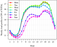
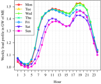
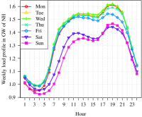
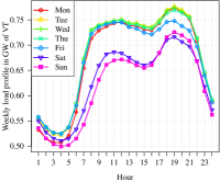
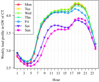
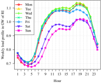
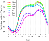
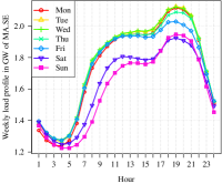
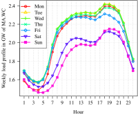
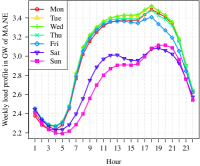
Figure 2: Weekly load profile for all ten zones in consideration in the ordering TOTAL, ME, NH, VT, CT, RI, MA, MA.SE, MA.WC and MA.NE.

Figure 3 shows the ISO New England zone (TOTAL) load and temperature data for the most recently available year. The figure depicts clearly a usual annual pattern. The load level peaks in winter and summer times. The former peak can be explained by higher needs in heating and illumination, the latter by a surge in the demand for air cooling.

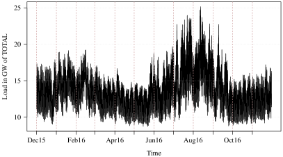
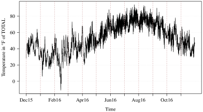
Figure 3: Load (left) and temperature (right) data from Dec 2015 to Nov 2016. This period is the last year of available data for the region TOTAL for the first task.

We have observed that the data exhibits annual and weekly seasonal patterns. Finally, we want to illustrate that there are so-called interaction effects between both seasonalities. Essentially, this means that the weekly (including the daily) periodic pattern is changing its shape over the year. To visualize this effect we transform the load data with respect to annual time periodicity into polar coordinates. Hence, we consider

$$\ell_{\text{x},i,t}=\ell_{i,t}\cos\left(\frac{2\pi t}{24A}\right)\ \ \text{ and }\ \ \ell_{\text{y},i,t}=\ell_{i,t}\sin\left(\frac{2\pi t}{24A}\right)$$

where $24A=24\times 365.24$ is the (meteorologic) period of a year.

Figure 4 plots $\ell_{\text{x},i,t}$ and $\ell_{\text{y},i,t}$ and thus visualizes the data in a form analogous to that of a wind rose popular in wind energy forecasting. The (Euclidean) distance to the center of the figure is the load level of the corresponding load value. The angle represents the time of the year, the four seasons match the four quadrants. We also highlight the hours of the day using different colors to put emphasis on interaction effects. We observe that the lower load values (those which are closer to the origin) occur during the night hours throughout the year. In summer (also late spring and early fall) we sometimes observe very extreme load values, also known as peaks. These peaks can occur at all day hours from around 9am to 9pm. In winter (also late fall) we similarly see large load values of around 20GW. However, in contrast to the summer peaks, they always occur during late afternoon and evening hours from around 4pm to 9pm. Hence, we can conclude that the structure of the weekly (including the daily) pattern changes over the year. Therefore, we have to take into account this effect when developing the forecasting model.

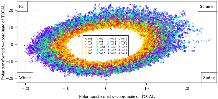
Figure 4: Polar transformed load data $\ell_{\text{x},i,t}$ and $\ell_{\text{y},i,t}$ in GW with respect to annual periodicity of TOTAL with hours of the day and seasons marked in different colors

Finally, we employ the logarithm of the load data for the main parts of the modeling procedure. Thus, we introduce $L_{i,t}=\log(\ell_{i,t})$ as log-load where we use MW as original unit for $\ell_{i,t}$.

4 The modeling and forecasting methodology

As mentioned previously, we model each load time series individually, i.e. we ignore the hierarchical structure. Note that incoherency in the load forecasting regarding the hierarchical structure is not penalized by the evaluation score. More details on coherent probabilistic load forecasts can be found in Taieb et al., (2017).

Thus, for each region $i$, the load $\ell_{i,t}$ (or log-load $L_{i,t}$) is modeled in exactly the same way. Therefore, we drop for convenience the index $i$ in the modeling and forecasting part.

A key element of the considered methodology is the decomposition of $L_{t}$ into a long-term trend component and a more stable component $Y_{t}$:

$$L_{t}=\text{trend}_{t}+Y_{t}.$$ (2)

This transformation is motivated from the stochastic point of view by the fact that $Y_{t}$ is closer than $L_{t}$ to a (periodically) stationary process. This simplifies the forthcoming analysis substantially. The long term trend component, $\text{trend}_{t}$, is modeled by a (smoothing) moving average type model. The main term, $Y_{t}$, is described by a simple quantile regression model.

4.1 The long term trend model

The trend component is not just modeled by a simple linear trend $\beta_{0}+\beta_{1}t$ but by a specific (smoothing) moving average type model. Therefore, we consider first the linear regression

$$L_{t}=\boldsymbol{\beta}^{\prime}\boldsymbol{X}_{t}+\epsilon_{t}$$ (3)

with $\boldsymbol{\beta}$ as a parameter vector, $\epsilon_{t}$ as an error term and $\boldsymbol{X}_{t}$ as a regression matrix containing daily/weekly dummies, annually periodic basis functions such as temperature impacts. Formally, we have

$$\boldsymbol{\beta}^{\prime}\boldsymbol{X}_{t}=\underbrace{\boldsymbol{\beta}_{1}{\mathcal{W}}_{t}+\sum_{j=1}^{4}\boldsymbol{\beta}_{1+j}{\mathcal{A}}^{\text{FB2}}_{t,j}{\mathcal{W}}_{t}+\sum_{j=1}^{11}\boldsymbol{\beta}_{5+j}{\mathcal{A}}^{\text{BS12}}_{t,j}{\mathcal{H}}_{t}}_{\text{periodically deterministic time effects}}+\underbrace{\boldsymbol{\beta}_{17}{\mathcal{T}}_{t}+\sum_{j=1}^{4}\boldsymbol{\beta}_{17+j}{\mathcal{A}}^{\text{FB2}}_{t,j}{\mathcal{T}}_{t}}_{\text{temperature effects}}$$ (4)

where ${\mathcal{T}}_{t}=(T_{t},T_{t}^{2},T_{t}^{3})^{\prime}$ is a vector with the first three temperature polynomials, ${\mathcal{H}}_{t}$ is a vector of length $24$ which includes all 24 hour-of-the-day dummies, ${\mathcal{W}}_{t}$ is a vector of length $24\times 7=168$ which contains all 168 hour-of-the-week dummies, ${\mathcal{A}}^{\text{FB2}}_{t}$ is a Fourier basis with annual periodicity of order 2 and ${\mathcal{A}}^{\text{BS12}}_{t}$ is cubic B-spline basis on an equidistant grid with 12 basis functions. All these components except the temperature part occur in the model description of $Y_{t}$ too and will be explained there in more detail. The polynomial temperature structure is assumed in many simple structured models, e.g. in Ziel et al., (2016). We consider a periodic cubic B-spline to benefits from the locality property. However, for $n$ Therefore we consider a mixture of periodic B-splines and Fourier-basis. However, considering only B-splines would have likely given similar results. Note that the last (12th) periodic B-spline component is dropped due to its collinearity with the day of the week dummy component. The overall parameter vector is $\boldsymbol{\beta}=(\boldsymbol{\beta}_{1},\boldsymbol{\beta}_{2},\ldots,\boldsymbol{\beta}_{21})^{\prime}$ where the vectors $\boldsymbol{\beta}_{i}$ have fitting model dimensions.

We estimate the linear regression equation (3) by ordinary least squares (OLS) using the given input data. This yields directly the residuals $\widehat{\epsilon}_{t}$ which we use for the estimation of the trend model.

The model for $\text{trend}_{t}$ is an annual (smoothing) moving average of $\epsilon_{t}$ given by

$$\text{trend}_{t}=\frac{1}{K}\sum_{k=1}^{K}\epsilon_{t-k}+e_{t}$$

with $e_{t}$ as an error term and a moving average window of about a year, so $K=52\times 7\times 24=8736$. To calculate $K$ we use a multiple of $7$ to avoid potential bias due to the weekly periodicity in $\epsilon_{t}$. Given the above results, we can easily estimate $\text{trend}_{t}$ using the plug-in principle:

$$\widehat{\text{trend}}_{t}=\frac{1}{K}\sum_{k=1}^{K}\widehat{\epsilon}_{t-k}.$$

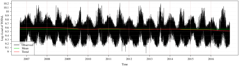
Figure 5: Log-load data $L_{t}$ (Observed, black) with its sample mean $\widehat{\mu}$ (Mean, green) and the estimated long-term trend plus sample mean component $\widehat{\text{trend}}_{t}+\widehat{\mu}$ (Trend, red).

In Figure 5 the estimate of the first task is visualized. There we see a downwards trend which is explained by $\widehat{\text{trend}}_{t}$. Moreover, we can vaguely see that for the first year the trend component is set to be constant (this can be better seen in Figure 6). Nevertheless, this has no impact on the current forecast.

The main purpose of removing the trend component is to create a more stationary type remainder process $Y_{t}$. If we would do only point forecasting, we could stop analyzing $\text{trend}_{t}$ as its forecast is simply the last known value. However, here we are interested in probabilistic forecasting. Thus, we have to take into account the uncertainty in the long-term component as well. To be more precise, we would like to know the quantiles $q_{\tau}(\text{trend}_{t_{\text{last}}+H})$ for all $\tau\in{\mathcal{Q}}$ at time $t_{\text{last}}+H$ within the out-of-sample range of interest where $t_{\text{last}}$ is the last in-sample time point and $H$ is the forecasting horizon. Here, we consider an extremely simple approach to estimate $q_{\tau}(\text{trend}_{t})$. We estimate it by taking the sample quantiles for each $\tau\in{\mathcal{Q}}$ of $\Delta_{H}\widehat{\text{trend}}_{t}=\widehat{\text{trend}}_{t}-\widehat{\text{trend}}_{t-H}$ within the in-sample period but ignore the first $K$ values as they are constant. Afterwards, we adjust the quantile forecasts by the corresponding median forecasts and add the last available trend value $\widehat{\text{trend}}_{t_{\text{last}}}$, as we assume that the median long-term trend is constant.

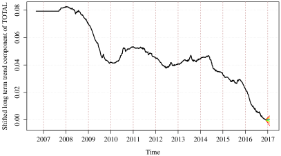
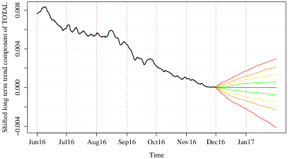
Figure 6: Long-term trend $\widehat{\text{trend}}_{t}$ shifted by $\widehat{\text{trend}}_{t_{\text{last}}}$ (black) with colored quantile forecasts of all $\tau\in{\mathcal{Q}}$ (0.1 and 0.9 red, 0.2 and 0.8 orange, 0.3 and 0.7 yellow, 0.4 and 0.6 green, 0.5 blue)

The corresponding result of task 1 is given in Figure 6 with the full in-sample period and only the last year of data. There we see that, compared to the 10 year in-sample period, the long term trend uncertainty is small as the forecasting horizon is relatively short. We also observe that the median forecast is fixed to be zero.

Note that from the theoretical point of view this approach is sloppy as we can not simply add quantile estimates to receive a consistent quantile estimate of $L_{t}$. However, we tested this procedure in out-of-sample test prior to the beginning of the competition and improved the forecasting accuracy in terms of the quantile loss.

4.2 The quantile regression model

For the remainder component $Y_{t}$ we exploit a simple quantile regression approach. However, instead of defining a single quantile regression, we consider 24 smaller models for each hour individually. For a more detailed discussion on this issue see Ziel and Weron, (2018). In turn, focusing on 24 models allows us to reduce computational costs and track the hourly specific structures in $Y_{t}$ more easily. To simplify notation we introduce the variable $Y_{d,h}$ which corresponds to the $Y_{t}$ value at hour $h$ and day $d$ (i.e. since $t=24(d-1)+h$). Similarly, this notation is used for all other objects (e.g. ${\mathcal{B}}_{d,h}$ for ${\mathcal{B}}_{t}$).

Remember that $Y_{d,h}$ carries all non-long term structures in the data, especially the annual, weekly and daily seasonal components. Hence, before we turn to the model definition, we denote another set of dummies, namely the day-of-the-week dummies. Thus, let ${\mathcal{D}}_{d}$ be a dummy vector of length $7$ with days of the week as its entries. Note that it holds that ${\mathcal{B}}_{d,h}=\text{vec}({\mathcal{H}}_{d,h}\otimes{\mathcal{D}}_{d})$, so the hour-of-the-week dummy basis is the vectorization of the outer product of the hour-of-the-week basis and the day-of-the-week basis.

As mentioned before, we consider a quantile regression model. Thus, we define a regression model for the quantile $q_{\tau}(Y_{d,h})$ for each $\tau\in{\mathcal{Q}}$. So the quantile regression model for $q_{\tau}(Y_{d,h})$ for each hour $h$ is given by

$$q_{\tau}(Y_{d,h})=\underbrace{\boldsymbol{\beta}_{\tau,h,1}{\mathcal{D}}_{d}}_{\text{day of the week effects}}+\underbrace{\sum_{j=1}^{4}\boldsymbol{\beta}_{\tau,h,1+j}{\mathcal{A}}^{\text{FB2}}_{d,h,j}{\mathcal{D}}_{d}}_{\text{annual effects with day of the week interaction}}+\underbrace{\sum_{j=1}^{11}\boldsymbol{\beta}_{\tau,h,5+j}{\mathcal{A}}^{\text{BS12}}_{d,h,j}}_{\text{annual effects}}+{\varepsilon}_{t}$$ (5)

The formula above implies that each quantile regression model has $46$ parameters, as the length of the vector $\boldsymbol{\beta}_{\tau,h}=(\boldsymbol{\beta}_{\tau,h,1},\ldots,\boldsymbol{\beta}_{\tau,h,16})^{\prime}$ equals to 46. The latter number can be calculated as follows. The vector $\boldsymbol{\beta}_{\tau,h,1}$ has the $7$ day-of-the-week dummy elements of ${\mathcal{D}}_{d}$. Then, since each of the vectors $\boldsymbol{\beta}_{\tau,h,2},\ldots,\boldsymbol{\beta}_{\tau,h,5}$ incorporates 7 factors, there are $4\times 7=28$ parameters for the annual-weekly interaction effects. Finally, there are 11 vectors $\boldsymbol{\beta}_{\tau,h,6},\ldots,\boldsymbol{\beta}_{\tau,h,16}$ of length 1 which account for the annual component. Through the above results it is clear that the number of the model parameters equals to $7+28+11=46$. Note that, analogously to the previous case, the last periodic B-spline component is dropped due to its collinearity with the day of the week dummies.

However, we observe that only three components in (5) characterize the full seasonal pattern. The day of the week effects are described by standard day of the week dummies with seven parameters. Thus, for every day of the week we assume a different load level.

The third term in (5) contains the periodic cubic B-splines with a periodicity of a (meteorologic) year ($A=365.24\times 24$). This term acts similarly to the monthly dummies but in a smooth manner, i.e. there is no abrupt jump if the month changes. To be able to achieve a higher performance of the constructed model, it is important that we extend the latter with a periodically smooth basis. Naturally, a simple Fourier basis which is based upon sine and cosine functions can do a similar job. Still, the locality property of the B-splines are their advantage. Note that the locality property is especially plausible if we would like to consider non-equidistant grids (e.g. to capture more distinct changes within the Christmas and New Years Day periods), but we refrain from doing so in this simple modeling approach. For more information on the construction and details of periodic B-splines we recommend Ziel and Liu, (2016) and Ziel et al., (2016).

Finally, there is the second term in (5) which models the interaction effect between the day of the week and annual seasonal components. Hence, this term describes how the weekly pattern is changing over the year. To capture this effect we simply multiply the day of the week basis functions ${\mathcal{D}}_{d}$ by an annual basis functions. Here we choose a Fourier basis of annual periodicity $A$ of order 2 (so it contains 2 sine and cosine waves of period $A$ and $A/2$). Similarly, to the case before, the periodic B-splines could be applied instead. Still, it is important that the number of parameters (here $4$) which describe the amount of annual components in the interaction effect is smaller than or at maximum equals to the plain (non-interactive) annual counterpart. This condition should be satisfied because the parameter space blows up speedily in response to a hike in the size of the interaction component. The correctness of this statement can be illustrated on the example of the current model: more than a half of all parameters (28 out of 46) come from the interaction component. Still, it appears rational to have at least four annual basis functions in the interaction component as we observe different effects during all four seasons, see Figure (4).

Note that the right hand side of (5) has the same structure as (4) except for the temperature components which are neglected. For many load forecasters it might sound counterintuitive that temperature effects are completely ignored here as the influence of temperature on electricity demand is often regarded as very important. However, this is only true for short term forecasting, where we have more accurate weather forecasts available. In turn, precision of the forecasts made for a longer horizon is poor. Therefore, the temperature carries only a small portion of relevant information for us. It is important to remember that all seasonal time-series information can be extracted without using temperature data, for example we can easily infer that the electricity demand is higher in winter than in spring just by studying load data (and its derivatives like $Y_{d,h}$). Because of similar reasons, we do not include any autoregressive components into the model, as we assume that the autoregressive memory is too weak on a forecasting horizon of at least a month. This implies that we can not substantially improve the forecasting accuracy by incorporating autoregressive effects.

Given the model specification in (5), we can easily estimate the $24\times 9\times 10$ (hours$\times$quantile levels$\times$zones) quantile regressions. Here the parameters $\boldsymbol{\beta}_{\tau,h}$ are optimized such that that the pinball score $S_{\tau}$ in (1) (or quantile loss) of $\boldsymbol{\beta}_{\tau,h}^{\prime}\boldsymbol{X}_{d,h}$ becomes minimal with respect to $Y_{d,h}$ over the full in-sample period. Formally, we get the quantile estimator by minimizing the following expression

$$\widehat{\boldsymbol{\beta}}_{\tau,h}=\operatorname*{arg\,min}_{\boldsymbol{\beta}}\sum_{d\in{\mathcal{D}}_{\text{InSample}}}S_{\tau}(Y_{d,h},\boldsymbol{\beta}^{\prime}\boldsymbol{X}_{d,h})$$ (6)

where ${\mathcal{D}}_{\text{InSample}}$ is the set of all in-sample days. We estimate the coefficients in (6) by noting that the minimization problem in (6) is equivalent to maximum likelihood estimation of the linear regression problem $Y_{d,h}=\boldsymbol{\beta}_{h}^{\prime}\boldsymbol{X}_{d,h}+{\varepsilon}_{d,h}$ where the error term ${\varepsilon}_{d,h}$ is assumed to follow an asymmetric Laplace distribution with skewness parameter $\tau$.

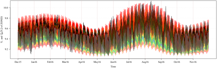
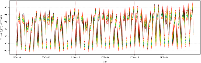
Figure 7: Observed log-load (black) with colored quantile fits of all quantiles $\tau\in{\mathcal{Q}}$ (0.1 and 0.9 red, 0.2 and 0.8 orange, 0.3 and 0.7 yellow, 0.4 and 0.6 green, 0.5 blue) for the most recent year and the most recent six weeks of ZONES.

For the implementation the outlined model above we consider the R-package quantreg (see Koenker, (2018)) with default inputs. Figure 7 shows the in-sample fit of the most recent year and the most recent six weeks of the assumed quantile model (referred to as ZONES). We see that, in general, the fit seems to capture not only the annual but also the weekly seasonal effects well. Also, the seasonal interaction effect is visible: In October the forecast of the magnitude of the evening peak is much less distinct than at the end of November, so the weekly pattern changes smoothly and appreciably over the six weeks. The figure also demonstrates that the range of the 10% quantile to 90% quantile is roughly 0.1. In contrast, the corresponding 10%-90% quantile range for the two month ahead forecast of $\text{trend}_{t}$ is less than 0.008, see Figure 6. Thus, most of the uncertainty in the forecast will be driven by the quantile regression component $Y_{d,h}$.

Using the estimated parameter vector $\widehat{\boldsymbol{\beta}}_{\tau,h}$ we can compute the quantile forecasts of $Y_{d,h}$ for each model by evaluating $\widehat{\boldsymbol{\beta}}_{\tau,h}^{\prime}\boldsymbol{X}_{t}$ for time point $t$. As all regressors in $\boldsymbol{X}_{t}$ are deterministic we can directly compute the forecasts with a forecasting horizon of $D$ days. These forecasts are denoted by $\widehat{q}_{\tau}(Y_{d_{\text{last}}+D,h})$. In turn, the latter expression can be index converted to $\widehat{q}_{\tau}(Y_{t_{\text{last}}+H})$. Afterwards, we estimate the final quantile log-load forecast by adding the quantile forecasts of $Y_{t}$ and $\text{trend}_{t}$ along the formula $\widehat{q}_{\tau}(L_{t_{\text{last}}+H})=\widehat{q}_{\tau}(Y_{t_{\text{last}}+H})+\widehat{q}_{\tau}(\text{trend}_{t_{\text{last}}+H})$. As mentioned before, this summation of quantiles can be ambiguous (it is only correct if $\text{trend}_{t}$ and $Y_{t}$ are comonotone), but the method seems to work sufficiently well in application. This was also tested in preliminary back-testing studies prior to the start of the competition. Finally, quantiles are preserved by strictly monotonic transforms and the exponential function $\exp$ as inverse of the logarithm $\log$ is strictly increasing. Thus, we obtain the quantile forecast of the load $\ell_{t}$ given by $\widehat{q}_{\tau}(\ell_{t_{\text{last}}+H})=\exp(\widehat{q}_{\tau}(L_{t_{\text{last}}+H}))$.

Figure 8 shows the forecast of the ISO New England zone for the first task. As the most recently available data was that at the end of November this is a two month ahead forecast. However, only the forecast for the latter month is submitted and evaluated. To emphasize this and visualize the the obtained results we removed the forecast values for January. We observe that the overall load level increased from November to January as we would expect it due to a respective drop in average daily temperature. However, the forecasted weekly pattern seem to be quite stable over January. Nevertheless, in contrast to Figure 7 we observe a small tendency that the evening peak decreases slightly at the end of January. This can be possibly explained by the fact that temperatures are starting to become warmer and the duration of the daylight increases. As a consequence, less electricity is being demanded.

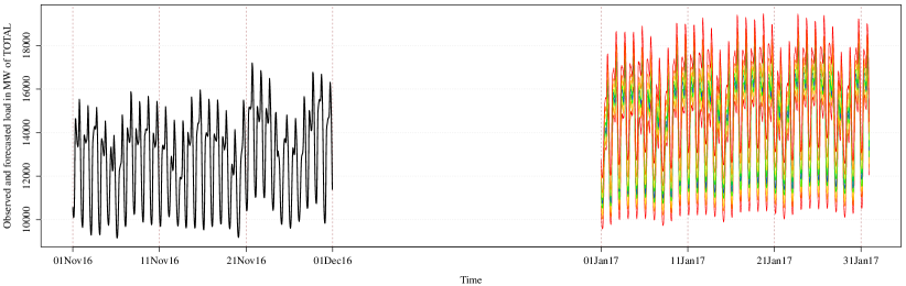
Figure 8: Observed load (black) and forecasted load (colored) for all quantiles $\tau\in{\mathcal{Q}}$ (0.1 and 0.9 red, 0.2 and 0.8 orange, 0.3 and 0.7 yellow, 0.4 and 0.6 green, 0.5 blue) for the first task.

5 Results and Conclusion

The proposed methodology allowed us to take 2nd place in the open data track and 4th place in the definite data track. In both tracks, only five teams succeed to achieve this excellent level of performance.

In Table 1 we show the overall results in terms of the pinball score for each task and each zone for the proposed model. There we also give the results of the Vanilla Benchmark (fore more details on the Vanilla Benchmark see Hong et al., (2016)) which is used in the final evaluation. Next to the pinball scores we highlight in Table 1 the improvement in the pinball score with respect to the benchmark. We see that in 90% of all cases the pinball score is smaller than the Vanilla benchmark. Given the simplicity of the model we developed, its forecasting accuracy appears remarkable and shows a high potential of the quantile regression methodology.

#	PB Score	TOTAL	ME	NH	VT	CT	RI	MASS	MA.SE	MA.WC	MA.NE
	Model (MW)	358.44	23.33	35.97	20.69	106.82	22.38	160.72	43.24	49.56	71.01
1	Benchmark (MW)	402.68	36.95	41.91	22.44	114.88	23.32	170.20	44.11	50.58	77.85
	Improvement (%)	$\pagecolor[rgb]{0.482,0.891,0.391}10.99$	$\pagecolor[rgb]{0.361,0.831,0.331}36.87$	$\pagecolor[rgb]{0.467,0.884,0.384}14.16$	$\pagecolor[rgb]{0.497,0.898,0.398}7.79$	$\pagecolor[rgb]{0.509,0.902,0.402}7.02$	$\pagecolor[rgb]{0.719,0.944,0.444}4.01$	$\pagecolor[rgb]{0.61,0.922,0.422}5.57$	$\pagecolor[rgb]{0.861,0.972,0.472}1.98$	$\pagecolor[rgb]{0.858,0.972,0.472}2.02$	$\pagecolor[rgb]{0.492,0.896,0.396}8.78$
	Model (MW)	369.05	22.72	31.65	14.91	111.28	24.56	179.17	48.75	58.29	75.29
2	Benchmark (MW)	401.51	29.11	35.34	15.49	115.72	24.18	190.36	50.69	60.32	81.02
	Improvement (%)	$\pagecolor[rgb]{0.496,0.898,0.398}8.08$	$\pagecolor[rgb]{0.431,0.865,0.365}21.95$	$\pagecolor[rgb]{0.485,0.892,0.392}10.44$	$\pagecolor[rgb]{0.736,0.947,0.447}3.77$	$\pagecolor[rgb]{0.732,0.946,0.446}3.83$	$\pagecolor[rgb]{1,0.922,0.5}-1.55$	$\pagecolor[rgb]{0.589,0.918,0.418}5.88$	$\pagecolor[rgb]{0.732,0.946,0.446}3.83$	$\pagecolor[rgb]{0.764,0.953,0.453}3.37$	$\pagecolor[rgb]{0.505,0.901,0.401}7.07$
	Model (MW)	369.05	22.72	31.65	14.91	111.28	24.56	179.17	48.75	58.29	75.29
3	Benchmark (MW)	401.51	29.11	35.34	15.49	115.72	24.18	190.36	50.69	60.32	81.02
	Improvement (%)	$\pagecolor[rgb]{0.496,0.898,0.398}8.08$	$\pagecolor[rgb]{0.431,0.865,0.365}21.95$	$\pagecolor[rgb]{0.485,0.892,0.392}10.44$	$\pagecolor[rgb]{0.736,0.947,0.447}3.77$	$\pagecolor[rgb]{0.732,0.946,0.446}3.83$	$\pagecolor[rgb]{1,0.922,0.5}-1.55$	$\pagecolor[rgb]{0.589,0.918,0.418}5.88$	$\pagecolor[rgb]{0.732,0.946,0.446}3.83$	$\pagecolor[rgb]{0.764,0.953,0.453}3.37$	$\pagecolor[rgb]{0.505,0.901,0.401}7.07$
	Model (MW)	346.68	23.52	30.37	20.33	95.81	20.34	173.63	47.63	53.84	73.48
4	Benchmark (MW)	351.89	23.96	29.43	21.07	98.91	21.54	175.86	49.62	55.43	73.32
	Improvement (%)	$\pagecolor[rgb]{0.896,0.979,0.479}1.48$	$\pagecolor[rgb]{0.872,0.974,0.474}1.83$	$\pagecolor[rgb]{1,0.841,0.5}-3.18$	$\pagecolor[rgb]{0.755,0.951,0.451}3.50$	$\pagecolor[rgb]{0.78,0.956,0.456}3.14$	$\pagecolor[rgb]{0.609,0.922,0.422}5.59$	$\pagecolor[rgb]{0.911,0.982,0.482}1.27$	$\pagecolor[rgb]{0.719,0.944,0.444}4.01$	$\pagecolor[rgb]{0.8,0.96,0.46}2.86$	$\pagecolor[rgb]{1,0.989,0.5}-0.22$
	Model (MW)	346.68	23.52	30.37	20.33	95.81	20.34	173.63	47.63	53.84	73.48
5	Benchmark (MW)	351.70	23.88	29.64	20.92	98.80	21.53	175.86	49.51	55.25	73.16
	Improvement (%)	$\pagecolor[rgb]{0.9,0.98,0.48}1.43$	$\pagecolor[rgb]{0.895,0.979,0.479}1.50$	$\pagecolor[rgb]{1,0.878,0.5}-2.45$	$\pagecolor[rgb]{0.804,0.961,0.461}2.81$	$\pagecolor[rgb]{0.788,0.958,0.458}3.03$	$\pagecolor[rgb]{0.612,0.922,0.422}5.54$	$\pagecolor[rgb]{0.911,0.982,0.482}1.27$	$\pagecolor[rgb]{0.734,0.947,0.447}3.80$	$\pagecolor[rgb]{0.822,0.964,0.464}2.55$	$\pagecolor[rgb]{1,0.978,0.5}-0.44$
	Model (MW)	180.12	15.78	15.67	14.45	49.05	10.34	93.20	30.01	31.35	37.07
6	Benchmark (MW)	202.83	29.71	16.74	17.23	55.11	11.19	106.5	34.19	34.91	44.41
	Improvement (%)	$\pagecolor[rgb]{0.481,0.891,0.391}11.19$	$\pagecolor[rgb]{0.315,0.807,0.307}46.89$	$\pagecolor[rgb]{0.551,0.91,0.41}6.42$	$\pagecolor[rgb]{0.458,0.879,0.379}16.12$	$\pagecolor[rgb]{0.482,0.891,0.391}11.00$	$\pagecolor[rgb]{0.498,0.899,0.399}7.60$	$\pagecolor[rgb]{0.475,0.888,0.388}12.49$	$\pagecolor[rgb]{0.476,0.888,0.388}12.24$	$\pagecolor[rgb]{0.486,0.893,0.393}10.21$	$\pagecolor[rgb]{0.456,0.878,0.378}16.53$

Table 1: Pinball (PB) scores of the considered model and the benchmark with corresponding improvement for all 6 tasks for all 10 zones.

More advanced effects, e.g. non-linear effects, public holidays effects or structural changes, were ignored in the present model. Incorporating structural changes in the long term trend appears to be the most prospective component which would likely boost the accuracy of a model. To show the correctness of the previous statement explicitly, consider, for example, that Massachusetts had a strong increase in solar power production in recent years, however, not as strong as the one recorded in Connecticut. This implies that not only the long term trend effect but also other model components vary over time. This can be seen especially clearly in summer periods, when the load volatility tends to be higher during the day hours due to stronger and less predictable meteorological impacts. Hence, including these effects would very likely improve the results substantially. Furthermore, we could also take into account the load time-series of other zones than the one we are actually forecasting, especially using the neighboring and hierarchical structure information might improve the forecasting performance.

Finally, there is always the curse of dimensionality in empirical data analytics to be acknowledged. Even though the considered models are still relatively low-dimensional, shrinkage algorithms are to be used to avoid the danger of overfitting. For quantile regression the quantile lasso is a plausible option to be applied in future. The R-package quantreg provides such an implementation.

References

References

- Gaillard et al., (2016) Gaillard, P., Goude, Y., and Nedellec, R. (2016). Additive models and robust aggregation for gefcom2014 probabilistic electric load and electricity price forecasting. International Journal of Forecasting, 32(3):1038–1050.
- Goude et al., (2014) Goude, Y., Nedellec, R., and Kong, N. (2014). Local short and middle term electricity load forecasting with semi-parametric additive models. IEEE transactions on smart grid, 5(1):440–446.
- Haben and Giasemidis, (2016) Haben, S. and Giasemidis, G. (2016). A hybrid model of kernel density estimation and quantile regression for GEFCom2014 probabilistic load forecasting. International Journal of Forecasting, 32(3):1017–1022.
- Hong et al., (2016) Hong, T., Pinson, P., Fan, S., Zareipour, H., Troccoli, A., and Hyndman, R. J. (2016). Probabilistic energy forecasting: Global energy forecasting competition 2014 and beyond. International Journal of Forecasting, 32(2):896–913.
- Koenker, (2018) Koenker, R. (2018). quantreg: Quantile Regression. R package version 5.35.
- Liu et al., (2017) Liu, B., Nowotarski, J., Hong, T., and Weron, R. (2017). Probabilistic load forecasting via quantile regression averaging on sister forecasts. IEEE Transactions on Smart Grid, 8(2):730–737.
- Maciejowska and Nowotarski, (2016) Maciejowska, K. and Nowotarski, J. (2016). A hybrid model for gefcom2014 probabilistic electricity price forecasting. International Journal of Forecasting, 32(3):1051–1056.
- Taieb et al., (2016) Taieb, S. B., Huser, R., Hyndman, R. J., and Genton, M. G. (2016). Forecasting uncertainty in electricity smart meter data by boosting additive quantile regression. IEEE Transactions on Smart Grid, 7(5):2448–2455.
- Taieb et al., (2017) Taieb, S. B., Taylor, J. W., and Hyndman, R. J. (2017). Coherent probabilistic forecasts for hierarchical time series. In International Conference on Machine Learning, pages 3348–3357.
- Ziel et al., (2016) Ziel, F., Croonenbroeck, C., and Ambach, D. (2016). Forecasting wind power–modeling periodic and non-linear effects under conditional heteroscedasticity. Applied Energy, 177:285–297.
- Ziel and Liu, (2016) Ziel, F. and Liu, B. (2016). Lasso estimation for gefcom2014 probabilistic electric load forecasting. International Journal of Forecasting, 32(3):1029–1037.
- Ziel and Weron, (2018) Ziel, F. and Weron, R. (2018). Day-ahead electricity price forecasting with high-dimensional structures: Univariate vs. multivariate modeling frameworks. Energy Economics, 70:396–420.