Novel all loop actions of interacting CFTs:
Construction, integrability and RG flows

George Georgiou^1,2 and  Konstantinos Sfetsos¹

¹Department of Nuclear and Particle Physics,
Faculty of Physics, National and Kapodistrian University of Athens,
Athens 15784, Greece

²Institute of Nuclear and Particle Physics,
National Center for Scientific Research Demokritos,
Ag. Paraskevi, GR-15310 Athens, Greece

georgiou@inp.demokritos.gr, ksfetsos@phys.uoa.gr

Abstract

We construct the all loop effective action representing, for small couplings, simultaneously self- and mutually interacting current algebra CFTs realized by WZW models. This non-trivially generalizes our previous works where such interactions were, at the linear level, not simultaneously present. For the two coupling case we prove integrability and calculate the coupled RG flow equations. We also consider non-Abelian T-duality type limits. Our models provide concrete realisations of integrable flows between exact CFTs and exhibit several new features which we discuss in detail.

1 Introduction

The purpose of the present work is to derive the all-loop effective action and study important properties such as integrability and the behavior under the renormalization group (RG) flow, of a class of theories based on WZW models for a group $G$ which encompasses and further generalizes all previous works in this research direction. Such models deviate from the conformal point in a way that can be quite involved. For small values of the coupling constants the deviation is driven by bilinears of the WZW model chiral and anti-chiral currents, denoted by $J^{a}_{\pm}$, where $a=1,2,\dots,\dim G$. These perturbations drive the theory away from the conformal point since they are generically not exactly marginal. Their form may serve also to distinguish between the different type of models existing in the literature and also singles out the present work in comparison with previous ones.

The first such example was worked out in [1] where the unperturbed conformal field theory (CFT) was a single WZW model for a group $G$ and level $k$ for the corresponding current algebra. In this case the perturbation contains terms proportional to

$$J^{a}_{+}J^{b}_{-}\ .$$ (1.1)

The currents belong to the same original CFT, so that this is a theory of self-interactions.

The next natural step in this program was to consider the case in which the original CFT is composed by two WZW models with currents $J^{a}_{i\pm}$, with $i=1,2$ and the perturbation being a linear combination of the two current bilinears of the form

$$J^{a}_{1+}J^{b}_{2-}\ ,\qquad J^{a}_{2+}J^{b}_{1-}\ .$$ (1.2)

Such perturbations presents a mutual interaction of the two WZW model theories and there are no self-interaction terms of currents in the same WZW model. The effective action for this case was constructed for equal current algebra levels in [2] and extended to the unequal level case in [3] which, although technically similar to the equal level case, encodes some new important physical features. An extension of these with several WZW models mutually interacting was constructed in [4].

These models were generically called $\lambda$-deformed from the letter-symbol $\lambda_{ab}$ used for the coefficients multiplying the perturbative terms in (1.1) and (1.2). Beyond the linear level the effective actions [1] and [2, 3] have of course non-trivial dependence on these $\lambda$-parameters.

Although the $\sigma$-model all-loop effective actions corresponding to the perturbations (1.1) and (1.2) are different, certain quantum characteristics of the models, concerning in particular the renormalization group (RG) are the same or closely related. To explain that, let us first recall that the RG flow equations for the $\sigma$-model of [1] were computed, exactly in $\lambda$ and for large $k$, using gravitational methods [5, 6] with results in perfect agreement with those obtained in the past using field theoretical methods [7, 8, 9] and more recently in [10]. In addition, all-loop correlators of current and primary field operators have been computed in [11, 12, 13]. In these computations a few terms obtained using perturbation theory and the non-perturbative symmetry, argued via path integral considerations in [14], were enough to obtain the exact results. In addition, for the $\sigma$-model of [2, 3] the anomalous dimensions of current and primaries in this theory were computed using CFT techniques in a field theoretical approach and symmetry arguments in [15]. As it turns out the $\beta$-functions for the couplings are identical to those of several non-coupled single $\lambda$-deformed models. Also, the anomalous dimensions of currents are related, though for the anomalous dimensions of generic primary field operators the results differ. The reason for such remarkable agreements is the fact that from a CFT point of view each of the two terms in (1.2) is the same as the one in (1.1) and moreover these two terms have vanishing operator product expansion (OPE), i.e. are mutually non-interacting. Hence, the corresponding couplings constants run independently under the RG flow and similar arguments can be made for the anomalous dimensions. In further support of the above, one can show [4] that the effective action of [2] is canonically equivalent to the sum of two actions as in [1].

We note that the most general expressions for the $\beta$-functions and anomalous dimensions for the operator driving the perturbation can be found in [16]. This includes the most general coupling matrix $\lambda_{ab}$ and having different levels for the chiral and anti-chiral currents. Remarkably, the above developments allowed the computation of Zamolodchikov’s $C$-function [17] exactly in the deformation parameter for the case of isotropic perturbations and to leading order in $k$ in [18]. The similarities mentioned above for the models corresponding to (1.1) and (1.2) extend to this case as well, the reason being the close relation of the $\beta$- and $C$-functions [17].

There were many other parallel developments or closely related to the above. Of particular importance is the extension to cases where the unperturbed CFT of a single WZW model is replaced by a coset CFT [1, 19, 20, 21]. The corresponding analysis for the case of supergroups was considered in [19, 20]. In addition, though integrability has not been a key factor in the computation of the $\beta$-functions and of the operators anomalous dimensions, in the case of isotropic deformations the above models have been demonstrated to be integrable [1, 19, 20, 22], [21] and [2, 3]. For the particular case of the isotropic deformation based on $SU(2)$ this has been proven before in [23]. Integrability was shown to persist in some other cases with more deformation parameters [24, 25]. Furthermore, deformed models of low dimensionality have been embedded to supergravity [26, 27, 28, 29]. Moreover, $\lambda$-deformations are related via Poisson-Lie T-duality, introduced for group spaces in [30] and extended for coset spaces in [31], and appropriate analytic continuations [32, 33], [25, 34, 35, 36] to $\eta$-deformations for group and coset spaces which were introduced in [37, 38, 39] and [40, 41, 42], respectively. The dynamics of scalar fields in some $\lambda$-deformed geometries corresponding to coset CFTs has been discussed in [43], the relation to Chern-Simons theories in [44] and D-branes in the context of $\lambda$-deformations in [45].

A very important remaining question is to construct a theory in which all current bilinears constructed form the original CFT based on two WZW models play rôle in the perturbation, that is all terms of the following type are present at the linear level and on equal footing

$$J^{a}_{1+}J^{b}_{1-}\ ,\qquad J^{a}_{2+}J^{b}_{2-}\ ,\qquad J^{a}_{1+}J^{b}_{2-}\ ,\qquad J^{a}_{2+}J^{b}_{1-}\ .$$ (1.3)

In this paper we overtake precisely this task and construct in section 2 the effective action taking into account all loop effects corresponding to the simultaneous presence of all of the above perturbations, self as well as mutual. In this case all terms have non-vanishing OPEs with each other at a sufficiently high order in perturbation theory. Therefore it its expected that the $\beta$-functions and anomalous dimensions for the operators will generically depend on all coupling constants. We focus for simplicity to a particular two parameter model case. We will provide a proof that the model is integrable and we will construct a non-Abelian T-duality limit in section 3. In section 4 we will derive and study in detail the RG flow equations for these couplings. We conclude the paper in section 5.

2 The Lagrangian and the equations of motion

In this section we construct our effective actions and the corresponding equations of motion.

Consider the group elements $g_{i}$, $i=1,2$ in a group $G$ and the corresponding actions for two WZW models at levels $k_{1}$ and $k_{2}$. We add to them the action of two PCMs which are mutually interacting and are constructed by two group elements $\tilde{g}_{i}$, $i=1,2$ in the same group $G$. Namely, we have that

$$\begin{split}&S_{k_{i},E_{i}}(g_{i},\tilde{g}_{i})=S_{k_{1}}(g_{1})+S_{k_{2}}(g_{2})-{1\over\pi}\int d^{2}\sigma\ \Big{(}\tilde{g}_{1}^{-1}\partial_{+}\tilde{g}_{1}E_{1}\tilde{g}_{1}^{-1}\partial_{-}\tilde{g}_{1}\\ &\qquad\qquad+\tilde{g}_{1}^{-1}\partial_{+}\tilde{g}_{1}E_{2}\tilde{g}_{2}^{-1}\partial_{-}\tilde{g}_{2}+\tilde{g}_{2}^{-1}\partial_{+}\tilde{g}_{2}E_{3}\tilde{g}_{1}^{-1}\partial_{-}\tilde{g}_{1}+\tilde{g}_{2}^{-1}\partial_{+}\tilde{g}_{2}E_{4}\tilde{g}_{2}^{-1}\partial_{-}\tilde{g}_{2}\Big{)}\ ,\end{split}$$ (2.1)

where the $E_{i}$, $i=1,2,3,4$ are generic coupling matrices. In the spirit of [1, 2] we gauge the global symmetry acting on the group elements as $g_{i}\to\Lambda_{i}^{-1}g_{i}\Lambda_{i}$ and $\tilde{g}_{i}\to\Lambda_{i}^{-1}\tilde{g}_{i}$, $i=1,2$. Hence, we will consider the gauge invariant action

$$S_{k_{i},E_{i}}(g_{i},\tilde{g}_{i},A_{\pm},B_{\pm})=S_{k_{1}}(g_{1},A_{\pm})+S_{k_{2}}(g_{2},B_{\pm})-{1\over\pi}\int d^{2}\sigma\ \Big{(}\tilde{g}_{1}^{-1}D_{+}\tilde{g}_{1}E_{1}\tilde{g}_{1}^{-1}D_{-}\tilde{g}_{1}$$

$$\qquad\ +\tilde{g}_{1}^{-1}D_{+}\tilde{g}_{1}E_{2}\tilde{g}_{2}^{-1}D_{-}\tilde{g}_{2}+\tilde{g}_{2}^{-1}D_{+}\tilde{g}_{2}E_{3}\tilde{g}_{1}^{-1}D_{-}\tilde{g}_{1}+\tilde{g}_{2}^{-1}D_{+}\tilde{g}_{2}E_{4}\tilde{g}_{2}^{-1}D_{-}\tilde{g}_{2}\Big{)}\ ,$$ (2.2)

where the standard gauged WZW action is

$$\begin{split}&S_{k_{1}}(g_{1},A_{\pm})=S_{k_{1}}(g_{1})+{k_{1}\over\pi}\int d^{2}\sigma\ {\rm Tr}\big{(}A_{-}\partial_{+}g_{1}g_{1}^{-1}-A_{+}g_{1}^{-1}\partial_{-}g_{1}\\ &\qquad\qquad\qquad+A_{-}g_{1}A_{+}g_{1}^{-1}-A_{-}A_{+}\big{)}\end{split}$$ (2.3)

and similarly for $S_{k_{2}}(g_{2},B_{\pm})$. The covariant derivatives are defined as $D_{\pm}\tilde{g}_{1}=(\partial_{\pm}-A_{\pm})\tilde{g}_{1}$ and $D_{\pm}\tilde{g}_{2}=(\partial_{\pm}-B_{\pm})\tilde{g}_{2}$. After fixing the gauge in (2) as $\tilde{g}_{1}=\tilde{g}_{2}=\mathbb{1}$ we arrive at the following action

$$\begin{split}&S_{k_{i},\lambda_{i}}(g_{1},g_{2},A_{\pm},B_{\pm})=S_{k_{1}}(g_{1})+S_{k_{2}}(g_{2})\\ &\qquad\quad+{k_{1}\over\pi}\int d^{2}\sigma\ {\rm Tr}\big{(}A_{-}\partial_{+}g_{1}g_{1}^{-1}-A_{+}g_{1}^{-1}\partial_{-}g_{1}+A_{-}g_{1}A_{+}g_{1}^{-1}\big{)}\\ &\qquad\quad+{k_{2}\over\pi}\int d^{2}\sigma\ {\rm Tr}\big{(}B_{-}\partial_{+}g_{2}g_{2}^{-1}-B_{+}g_{2}^{-1}\partial_{-}g_{2}+B_{-}g_{2}B_{+}g_{2}^{-1}\big{)}\\ &\qquad\quad-{\sqrt{k_{1}k_{2}}\over\pi}\int d^{2}\sigma\ \Big{(}B_{+}\lambda_{1}^{-1}A_{-}+A_{+}\lambda_{2}^{-1}B_{-}+B_{+}\lambda_{3}^{-1}B_{-}+A_{+}\lambda_{4}^{-1}A_{-}\Big{)}\ ,\end{split}$$ (2.4)

where for later convenience we have redefined the coupling matrices appearing in the PCM models as

$$\begin{split}&\sqrt{k_{1}k_{2}}\ \lambda_{1}^{-1}=E_{3}\ ,\qquad\sqrt{k_{1}k_{2}}\ \lambda_{2}^{-1}=E_{2}\ ,\\ &\sqrt{k_{1}k_{2}}\ (\lambda_{3}^{-1}-\lambda_{0}^{-1})=E_{4}\ ,\qquad\sqrt{k_{1}k_{2}}\ (\lambda_{4}^{-1}-\lambda_{0})=E_{1}\ .\end{split}$$ (2.5)

In order to obtain the $\sigma$-model we can integrate out the gauge fields since they appear only quadratically. To do that we use their equations of motion which we prefer to present later in (2.13). In this way we find that

$$\begin{split}&A_{+}=i\Big{(}(\lambda_{0}\lambda_{3}^{-T}-D_{2})\lambda_{1}^{T}(\lambda_{0}^{-1}\lambda_{4}^{-T}-D_{1})-\lambda_{2}^{-T}\Big{)}^{-1}\Big{(}(\lambda_{0}\lambda_{3}^{-T}-D_{2})\lambda_{1}^{T}J_{1+}-\lambda_{0}^{-1}J_{2+}\Big{)}\ ,\\ &B_{+}=i\Big{(}(\lambda_{0}^{-1}\lambda_{4}^{-T}-D_{1})\lambda_{2}^{T}(\lambda_{0}\lambda_{3}^{-T}-D_{2})-\lambda_{1}^{-T}\Big{)}^{-1}\Big{(}(\lambda_{0}^{-1}\lambda_{4}^{-T}-D_{1})\lambda_{2}^{T}J_{2+}-\lambda_{0}J_{1+}\Big{)}\end{split}$$ (2.6)

and that

$$\begin{split}&A_{-}=-i\Big{(}(\lambda_{0}\lambda_{3}^{-1}-D_{2}^{T})\lambda_{2}(\lambda_{0}^{-1}\lambda_{4}^{-1}-D_{1}^{T})-\lambda_{1}^{-1}\Big{)}^{-1}\Big{(}(\lambda_{0}\lambda_{3}^{-1}-D_{2}^{T})\lambda_{2}J_{1-}-\lambda_{0}^{-1}J_{2-}\Big{)}\ ,\\ &B_{-}=-i\Big{(}(\lambda_{0}^{-1}\lambda_{4}^{-1}-D_{1}^{T})\lambda_{1}(\lambda_{0}\lambda_{3}^{-1}-D_{2}^{T})-\lambda_{2}^{-1}\Big{)}^{-1}\Big{(}(\lambda_{0}^{-1}\lambda_{4}^{-1}-D_{1}^{T})\lambda_{1}J_{2-}-\lambda_{0}J_{1-}\Big{)}\ .\end{split}$$ (2.7)

The definition of the matrices $D_{ab}$ and the currents $J^{a}_{\pm}$ is as follows

$$J^{a}_{+}=-i\,{\rm Tr}(t^{a}\partial_{+}gg^{-1}),\qquad J^{a}_{-}=-i\,{\rm Tr}(t^{a}g^{-1}\partial_{-}g)\ ,\qquad D_{ab}={\rm Tr}(t_{a}gt_{b}g^{-1})\ ,$$ (2.8)

where the $t^{a}$’s are Hermitian matrices obeying $[t_{a},t_{b}]=if_{ab}{}^{c}t_{c}$, for some real algebra structure constants. When a current or the orthogonal matrix $D$ has an index $1$ or $2$ this implies that one should use the corresponding group element in its definition. In addition, we have defined the ratio of the two levels

$$\lambda_{0}=\sqrt{{k_{1}\over k_{2}}}\ .$$ (2.9)

Substitution of the expressions for the gauge fields into (2.4) results into a $\sigma$-model action which can be written in matrix notation as

$$\begin{split}&S_{k_{i},\lambda_{i}}(g_{1},g_{2})=S_{k_{1}}(g_{1})+S_{k_{2}}(g_{2})\\ &+{1\over\pi}\int d^{2}\sigma\ \Big{[}k_{1}J_{1+}\Big{(}(\lambda_{0}\lambda_{3}^{-1}-D_{2}^{T})\lambda_{2}(\lambda_{0}^{-1}\lambda_{4}^{-1}-D_{1}^{T})-\lambda_{1}^{-1}\Big{)}^{-1}\Big{(}(\lambda_{0}\lambda_{3}^{-1}-D_{2}^{T})\lambda_{2}J_{1-}-\lambda_{0}^{-1}J_{2-}\Big{)}\\ &\quad+k_{2}J_{2+}\Big{(}(\lambda_{0}^{-1}\lambda_{4}^{-1}-D_{1}^{T})\lambda_{1}(\lambda_{0}\lambda_{3}^{-1}-D_{2}^{T})-\lambda_{2}^{-1}\Big{)}^{-1}\Big{(}(\lambda_{0}^{-1}\lambda_{4}^{-1}-D_{1}^{T})\lambda_{1}J_{2-}-\lambda_{0}J_{1-}\Big{)}\Big{]}\ .\end{split}$$ (2.10)

Note that, for $\lambda_{1,2}\to\infty$ one obtains two decoupled single $\lambda$-deformed models [1]. These can be most easily seen by taking this limit in (2.4) before integrating out the gauge fields. Hence, then (2.10) describes self-interactions for two decoupled WZW models which for small values of the remaining couplings $\lambda_{3,4}$ are of the form (1.1). On the other hand if $\lambda_{3,4}\to\infty$ one obtains the model of [2] corresponding for small values of $\lambda_{1,2}$ to mutual interactions of two WZW models of the form (1.2). This may also easily seen from inspecting (2.4).

By keeping all matrices one has the most general scenario. Indeed, if we take small values for the entries of the $\lambda$-matrices keeping nevertheless their ratios finite, we obtain that

$$\begin{split}&S_{k_{i},\lambda_{i}}(g_{1},g_{2})=S_{k_{1}}(g_{1})+S_{k_{2}}(g_{2})+{1\over\pi}\int d^{2}\sigma\ \Big{[}k_{1}\lambda_{0}M_{2}J_{1+}J_{1-}\\ &\qquad-k_{1}\lambda_{0}^{-1}M_{3}J_{1+}J_{2-}+k_{2}\lambda_{0}^{-1}M_{1}J_{2+}J_{2-}-k_{1}\lambda_{0}M_{4}J_{2+}J_{1-}\Big{]}+\cdots\ ,\end{split}$$ (2.11)

where we took for simplicity all the $\lambda$-matrices proportional to the identity and we have defined the constants

$$(M_{1},M_{2},M_{3},M_{4})={1\over\lambda_{1}\lambda_{2}-\lambda_{3}\lambda_{4}}(\lambda_{1}\lambda_{2}\lambda_{3},\lambda_{1}\lambda_{2}\lambda_{4},\lambda_{1}\lambda_{3}\lambda_{4},\lambda_{2}\lambda_{3}\lambda_{4})\ .$$ (2.12)

These constant couplings are small and of the same order of magnitude as the original $\lambda$’s. Hence, what drives the original CFT, which is given by the sum of the two WZW actions in (2.11), away from the conformal point is indeed a linear combination of all terms in (1.3) representing simultaneously self- and mutual-interactions.

We will write in some detail the equations of motion since this will be convenient in demonstrating that the theory described by the actions (2.4) and (2.10) is integrable for a particular case where two out of the four couplings are present.

Varying (2.4) with respect to $A_{\pm}$ and $B_{\pm}$ we find the following constraints

$$\begin{split}&D_{+}g_{1}\,g_{1}^{-1}=(\lambda_{0}^{-1}\lambda_{4}^{-T}-\mathbb{1})A_{+}+\lambda_{0}^{-1}\lambda_{1}^{-T}B_{+}\ ,\\ &g_{1}^{-1}D_{-}g_{1}=(\mathbb{1}-\lambda_{0}^{-1}\lambda_{4}^{-1})A_{-}-\lambda_{0}^{-1}\lambda_{2}^{-1}B_{-}\ ,\\ &D_{+}g_{2}\,g_{2}^{-1}=(\lambda_{0}\lambda_{3}^{-T}-\mathbb{1})B_{+}+\lambda_{0}\lambda_{2}^{-T}A_{+}\ ,\\ &g_{2}^{-1}D_{-}g_{2}=(\mathbb{1}-\lambda_{0}\lambda_{3}^{-1})B_{-}-\lambda_{0}\lambda_{1}^{-1}A_{-}\ ,\end{split}$$ (2.13)

where the covariant derivatives acting on the group elements are defined according to the transformation laws that leave (2) invariant. Namely, $D_{\pm}g_{1}=\partial_{\pm}g_{1}-[A_{\pm},g_{1}]$ and $D_{\pm}g_{2}=\partial_{\pm}g_{2}-[B_{\pm},g_{2}]$. By solving these for the gauge fields we obtain the solution (2.6) and (2.7) we have already presented. Varying the action with respect to group elements $g_{1}$ and $g_{2}$ results into

$$D_{-}(D_{+}g_{1}g_{1}^{-1})=F_{+-}^{(A)}\ ,\qquad D_{-}(D_{+}g_{2}g_{2}^{-1})=F_{+-}^{(B)}\ ,$$ (2.14)

where the field strenghts are defined as usual

$$F_{+-}^{(A)}=\partial_{+}A_{-}-\partial_{-}A_{+}-[A_{+},A_{-}]\ ,\qquad F_{+-}^{(B)}=\partial_{+}B_{-}-\partial_{-}B_{+}-[B_{+},B_{-}]\ .$$ (2.15)

Equivalently, the equations (2.14) can be written as

$$D_{+}(g_{1}^{-1}D_{-}g_{1})=F_{+-}^{(A)}\ ,\qquad D_{+}(g_{2}^{-1}D_{-}g_{2})=F_{+-}^{(B)}\ .$$ (2.16)

The next step is to substitute the constraint equations (2.13) in (2.14) and (2.16). After some algebra one obtains the following two sets of equations

$$\begin{split}&\partial_{+}A_{-}-\lambda_{0}^{-1}\lambda_{4}^{-T}\partial_{-}A_{+}-\lambda_{0}^{-1}\lambda_{1}^{-T}\partial_{-}B_{+}=\lambda_{0}^{-1}[\lambda_{4}^{-T}A_{+},A_{-}]+\lambda_{0}^{-1}[\lambda_{1}^{-T}B_{+},A_{-}]\ ,\\ &\partial_{+}B_{-}-\lambda_{0}\lambda_{3}^{-T}\partial_{-}B_{+}-\lambda_{0}\lambda_{2}^{-T}\partial_{-}A_{+}=\lambda_{0}[\lambda_{3}^{-T}B_{+},B_{-}]+\lambda_{0}[\lambda_{2}^{-T}A_{+},B_{-}]\ \end{split}$$ (2.17)

and

$$\begin{split}&\lambda_{0}^{-1}\lambda_{2}^{-1}\partial_{+}B_{-}-\partial_{-}A_{+}+\lambda_{0}^{-1}\lambda_{4}^{-1}\partial_{+}A_{-}=\lambda_{0}^{-1}[A_{+},\lambda_{4}^{-1}A_{-}]+\lambda_{0}^{-1}[A_{+},\lambda_{2}^{-1}B_{-}]\ ,\\ &\lambda_{0}\lambda_{1}^{-1}\partial_{+}A_{-}-\partial_{-}B_{+}+\lambda_{0}\lambda_{3}^{-1}\partial_{+}B_{-}=\lambda_{0}[B_{+},\lambda_{3}^{-1}B_{-}]+\lambda_{0}[B_{+},\lambda_{1}^{-1}A_{-}]\ .\end{split}$$ (2.18)

These are written solely in terms of the gauge fields and the group elements are implicitly present via (2.6) and (2.7).

The actions (2.4) and (2.10) as well as the set of equations of motion (LABEL:eomAinitial1) and (LABEL:eomAinitial2) are invariant under the $\mathbb{Z}_{2}$-symmetry

$$k_{1}\leftrightarrow k_{2}\ ,\quad\lambda_{1}\leftrightarrow\lambda_{2}\ ,\quad\lambda_{3}\leftrightarrow\lambda_{4}\ ,\quad A_{\pm}\leftrightarrow B_{\pm}\ ,\quad g_{1}\leftrightarrow g_{2}\ .$$ (2.19)

Due to this symmetry we may take $k_{1}\leqslant k_{2}$ with no loss of generality. In addition, the actions are invariant under the parity transformation

$$\begin{split}&+\leftrightarrow-\ ,\quad A_{+}\leftrightarrow A_{-}\ ,\quad B_{+}\leftrightarrow B_{-}\ ,\quad g_{i}\to g_{i}^{-1}\ ,\quad i=1,2\ ,\\ &\lambda_{1}\leftrightarrow\lambda_{2}^{T}\ ,\quad\lambda_{3}\to\lambda_{3}^{T}\ ,\quad\lambda_{4}\to\lambda_{4}^{T}\ ,\end{split}$$ (2.20)

upon which the equations (LABEL:eomAinitial1) and (LABEL:eomAinitial2) are interchanged.

We note the following interesting case. If we choose

$$\begin{split}&\lambda_{1}^{-1}=\lambda_{2}^{-1}={1\over 4}(1-\lambda^{-1})(\lambda_{0}+\lambda_{0}^{-1})\ ,\\ &\lambda_{3}^{-1}=\lambda_{4}^{-1}={1\over 4}\lambda_{0}^{-1}(\lambda^{-1}-1)+{1\over 4}\lambda_{0}(\lambda^{-1}+3)\ \end{split}$$ (2.21)

and after redefining $A_{\pm}\to A_{1\pm}$ and $B_{\pm}\to A_{2\pm}$ then the action (2.4) become that in Eq. (2.1) of [21]. It has been shown in that work that the corresponding $\sigma$-model action is the $\lambda$-deformation $G_{k_{1}}\times G_{k_{2}}/G_{k_{1}+k_{2}}$ coset CFT model and moreover it is an integrable one. Various other properties of this special $\lambda$-deformed models were worked out extensively in [21].

In the rest of the paper we will restrict ourselves to the isotropic case in which all coupling matrices are proportional to the identity, reserving nevertheless the same symbol of the proportionality constant, i.e.

$$(\lambda_{i})_{ab}=\lambda_{i}\delta_{ab}\ ,\quad\forall\ i=1,2,3,4\ .$$ (2.22)

3 Truncation to a two-parameter integrable model

In this section we discuss in detail a two-parameter model which arises by taking the limit $\lambda_{2},\lambda_{3}\to\infty$. We will see below in the calculations of the $\beta$-functions of the model that this is a consistent truncation of the full theory. From (2.4) we see that there is a term mixing $B_{+}$ and $A_{-}$. Hence, we expect that the resulting $\sigma$-model will describe self-interactions as well mutual ones. Indeed, the perturbation from the conformal point will be driven by the first and fourth bilinear in (1.3). Simple quantum field theoretical arguments show that the inclusion of third bilinear is not self-consistent at the quantum level and one necessarily has to include the remaining fourth bilinear as well.

3.1 Truncation of the action and the equations of motion

In the limit $\lambda_{2},\lambda_{3}\to\infty$. the action (2.10) takes the form

$$\begin{split}&S_{k_{1},k_{2}}(g_{1},g_{2})=S_{k_{1}}(g_{1})+S_{k_{2}}(g_{2})\\ &\qquad\qquad+{k_{1}\over\pi}\int d^{2}\sigma\ J_{1+}(\lambda_{0}^{-1}\lambda_{4}^{-1}\mathbb{1}-D_{1}^{T})^{-1}J_{1-}\\ &\qquad\qquad-{k_{2}\over\pi}\int d^{2}\sigma\ J_{2+}D_{2}J_{2-}\\ &\qquad\qquad+{k_{2}\over\pi}\lambda_{0}\lambda_{1}^{-1}\int d^{2}\sigma\ J_{2+}D_{2}(\lambda_{0}^{-1}\lambda_{4}^{-1}\mathbb{1}-D_{1}^{T})^{-1}J_{1-}\ .\end{split}$$ (3.1)

One observes that combining $S_{k_{2}}(g_{2})$ and the third line we obtain the WZW model action $S_{-k_{2}}(g_{2}^{-1})$ which has negative signature. To remedy the situation we perform the following redefinition of the couplings and analytic continuation in the specified order

$$\begin{split}&\lambda_{4}=\lambda_{0}^{-1}\lambda\ ,\quad\lambda_{1}=\lambda_{0}\lambda\tilde{\lambda}^{-1}\ ,\\ &{\rm then\ let}\ \ k_{2}\to-k_{2}\ ,\quad g_{2}\to g_{2}^{-1}\ .\end{split}$$ (3.2)

Then the action (3.1) becomes

$$\begin{split}&S_{k_{1},k_{2}}(g_{1},g_{2})=S_{k_{1}}(g_{1})+{k_{1}\over\pi}\int d^{2}\sigma\ J_{1+}(\lambda^{-1}\mathbb{1}-D_{1}^{T})^{-1}J_{1-}+S_{k_{2}}(g_{2})\\ &\qquad\qquad\qquad\ +{k_{2}\over\pi}\tilde{\lambda}\lambda^{-1}\int d^{2}\sigma\ J_{2+}(\lambda^{-1}\mathbb{1}-D_{1}^{T})^{-1}J_{1-}\ .\end{split}$$ (3.3)

The first line is the original $\lambda$-deformed model and a WZW model, whereas the second line represents their mutual interaction. Since the matrix $D_{1}$ is orthogonal it has eigenvalues lying on the unit circle. Therefore, to avoid singularities we restrict to $-1<\lambda<1$. Moreover, examining the determinant and the trace of the metric that can be extracted from (3.3) we find that Euclidean signature is guaranteed provided that the parameters $\lambda$ and $\tilde{\lambda}$ are such that they lie within the ellipsis, i.e.

$$\lambda^{2}+{k_{2}\over k_{1}}\tilde{\lambda}^{2}<1\ ,$$ (3.4)

in addition to $k_{1},k_{2}$ being positive integers. Note that since we have broken the $\mathbb{Z}_{2}$-symmetry by turning off two of the possible interacting terms between gauge fields in we cannot assume with no generality loss that one of the levels is larger than the other since that would have been a restriction of the possible parametric space. This will be important when we discuss the RG flows equations and the associated fixed points in section 4.

For small values of $\lambda$ and $\tilde{\lambda}$ we have that

$$\begin{split}&S_{k_{1},k_{2}}(g_{1},g_{2})=S_{k_{1}}(g_{1})+S_{k_{2}}(g_{2})\\ &\qquad\qquad+{k_{1}\over\pi}\lambda\int d^{2}\sigma\ J_{1+}J_{1-}+{k_{2}\over\pi}\tilde{\lambda}\int d^{2}\sigma\ J_{2+}J_{1-}+{\cal O}(\lambda^{2},\lambda\tilde{\lambda})\ .\end{split}$$ (3.5)

Hence we have simultaneously mutual as well as self-interactions between two WZW models. Thus (3.3) is the corresponding exact effective action in which all loop effects in $\lambda$ and $\tilde{\lambda}$ are taken into account. By construction gravity is trusted for small curvatures which is warranted as long as $k_{1},k_{2}\gg 1$.

One can show that the action (3.3) has the following non-perturbative in parameter space symmetry

$$g_{1}\to g_{1}^{-1}\ ,\quad\lambda\to{1\over\lambda}\ ,\quad k_{1}\to-k_{1}\ ,\quad\tilde{\lambda}\to\tilde{\lambda\over\lambda}\ .$$ (3.6)

This is an extension of the similar symmetry for the original $\lambda$-deformed theory [1] found in [14, 5] and of the similar ones in [2, 3] and [21]. This symmetry mixes the two coupling constants and it will be a symmetry of the $\beta$-functions which we will compute below in section 4. Moreover, it is expected to be a symmetry of the anomalous dimensions and of the correlation functions of the various operators in the theory as it happened in analogous computations in [11, 12] and [13].

The equations of motion for this two-parameter $\sigma$-model case can be obtained by taking the limit $\lambda_{2},\lambda_{3}\to\infty$ in the equations (LABEL:eomAinitial1) and (LABEL:eomAinitial2). The result is given by

$$\begin{split}&\lambda_{0}\lambda_{1}\lambda_{4}\partial_{+}A_{-}-\lambda_{4}\partial_{-}B_{+}-\lambda_{1}\partial_{-}A_{+}=\lambda_{4}[B_{+},A_{-}]+\lambda_{1}[A_{+},A_{-}]\ ,\\ &\partial_{+}B_{-}=0\ ,\\ &\partial_{+}A_{-}-\lambda_{0}\lambda_{4}\partial_{-}A_{+}=[A_{+},A_{-}]\ ,\\ &\lambda_{0}\partial_{+}A_{-}-\lambda_{1}\partial_{-}B_{+}=\lambda_{0}[B_{+},A_{-}]\ .\end{split}$$ (3.7)

After the redefinitions (3.2) these become

$$\begin{split}&-{k_{1}\over k_{2}}\lambda\partial_{+}A_{-}-\tilde{\lambda}\partial_{-}B_{+}+{k_{1}\over k_{2}}\partial_{-}A_{+}=\tilde{\lambda}[B_{+},A_{-}]-{k_{1}\over k_{2}}[A_{+},A_{-}]\ ,\\ &\partial_{+}B_{-}=0\ ,\\ &\partial_{+}A_{-}-\lambda\partial_{-}A_{+}=[A_{+},A_{-}]\ ,\\ &\tilde{\lambda}\partial_{+}A_{-}-\lambda\partial_{-}B_{+}=\tilde{\lambda}[B_{+},A_{-}]\ .\end{split}$$ (3.8)

Hence, the field $B_{-}$ decouples from the rest of the equations.

For $\tilde{\lambda}=\lambda$ the above system can be further simplified to

$$\begin{split}&\left(1+{k_{2}\over k_{1}}\right)\lambda\partial_{+}A_{-}-\partial_{-}A_{+}=[A_{+},A_{-}]\ ,\\ &\partial_{+}B_{-}=0\ ,\\ &\partial_{+}A_{-}-\lambda\partial_{-}A_{+}=[A_{+},A_{-}]\ ,\\ &\partial_{+}A_{-}-\partial_{-}B_{+}=[B_{+},A_{-}]\ .\end{split}$$ (3.9)

In that case the first and third equations are enough to determine $A_{\pm}$. Then the last equation can be integrated in order to obtain $B_{+}$.

These systems of equations, in particular (LABEL:eomAfinal1r), will be used next to show integrability of our two-parameter model.

3.2 Integrability

We will show that the above theory with two independent couplings $\lambda$ and $\tilde{\lambda}$ is integrable. To achieve this goal we should be able to derive the four equations of motion (LABEL:eomAfinal1r) from a Lax pair containing a spectral parameter. However, as it has been already mentioned, the second equation among them decouples since $B_{-}$ does not appear in any of the rest three equations. Furthermore, this equation implies chirality for $B_{-}$ hence implying an infinite number of conserved charges which can be constructed solely from $B_{-}$. It is, thus, enough to determine a Lax connection for the remaining three equations of motion.

To proceed we will assume that the Lax connection takes the following form

$$\begin{split}{\cal L}_{+}=uA_{+}+vB_{+},\qquad{\cal L}_{-}=\lambda^{-1}wA_{-},\end{split}$$ (3.10)

where $u,v$ and $w$ are constants depending on the couplings $\lambda$ and $\tilde{\lambda}$, as well as on the WZW levels $k_{1}$ and $k_{2}$ and the spectral parameter. The deformation parameter $\lambda$ has been introduced in the above expression for convenience. From the Lax equation

$$\partial_{+}{\cal L}_{-}-\partial_{-}{\cal L}_{+}-[{\cal L}_{+},{\cal L}_{-}]=0\ ,$$ (3.11)

one then obtains

$$\begin{split}\lambda^{-1}w\partial_{+}A_{-}-u\partial_{-}A_{+}-v\partial_{-}B_{+}-\lambda^{-1}uw[A_{+},A_{-}]-\lambda^{-1}vw[B_{+},A_{-}]=0\ .\end{split}$$ (3.12)

We may solve the system (LABEL:eomAfinal1r) in terms of the derivatives of the gauge fields to obtain that

$$\begin{split}&\partial_{+}A_{-}={1\over\Delta}\Big{(}k_{1}(1-\lambda)[A_{+},A_{-}]+k_{2}\tilde{\lambda}(\lambda-\tilde{\lambda})[B_{+},A_{-}]\Big{)}\ ,\\ &\partial_{-}A_{+}={1\over\lambda\Delta}\Big{(}\big{(}k_{2}\tilde{\lambda}^{2}-k_{1}\lambda(1-\lambda)\big{)}[A_{+},A_{-}]+k_{2}\tilde{\lambda}(\lambda-\tilde{\lambda})[B_{+},A_{-}]\Big{)}\ ,\\ &\partial_{-}B_{+}={\tilde{\lambda}\over\lambda\Delta}\Big{(}k_{1}(1-\lambda)[A_{+},A_{-}]+\big{(}k_{2}\lambda\tilde{\lambda}-k_{1}(1-\lambda^{2})\big{)}[B_{+},A_{-}]\Big{)}\ ,\end{split}$$ (3.13)

where we have defined the constant

$$\Delta=k_{1}(1-\lambda^{2})-k_{2}\tilde{\lambda}^{2}\ .$$ (3.14)

Substituting (LABEL:eom1-sol) into (3.12) results into two algebraic equations obtained by equating to zero the coefficients of the commutators $[A_{+},A_{-}]$ and $[B_{+},A_{-}]$. These are given by

$$\begin{split}&\big{[}k_{2}\tilde{\lambda}^{2}-k_{1}(1-\lambda^{2})\big{]}uw-\big{[}k_{2}\tilde{\lambda}^{2}-k_{1}\lambda(1-\lambda)\big{]}u+k_{1}(1-\lambda)(w-\tilde{\lambda}v)=0\ ,\\ &\big{[}k_{2}\tilde{\lambda}^{2}-k_{1}(1-\lambda^{2})\big{]}vw-\tilde{\lambda}\big{[}k_{2}\lambda\tilde{\lambda}-k_{1}(1-\lambda^{2})\big{]}v+k_{2}\tilde{\lambda}(\lambda-\tilde{\lambda})(w-u)=0\ .\end{split}$$ (3.15)

Obviously, satisfying this system leaves one parameter free among any combination of $u,v$ and $w$ which may serve as the spectral parameter of the Lax pair in (3.10). An explicit solution is obtained by solving (3.15) for $u$ and $v$ in terms of $w$ and identify the latter with the spectral parameter $z$. The result is

$$\begin{split}&{\cal L}_{+}={k_{1}(\lambda-1)z(z-\tilde{\lambda})\over Q}A_{+}-{k_{2}\tilde{\lambda}(\lambda-\tilde{\lambda})(z-1)z\over Q}B_{+},\qquad{\cal L}_{-}=\lambda^{-1}zA_{-}\\ &Q=k_{1}(\lambda-1)(\lambda(z-1)+z)(z-\tilde{\lambda})+k_{2}\tilde{\lambda}^{2}(z-1)(z-\lambda).\\ \end{split}$$ (3.16)

Note that for $\tilde{\lambda}=\lambda$ the Lax pair in (LABEL:Lax-final) has vanishing coefficient for $B_{+}$. This is consistent with the fact that in (LABEL:eomAfinal1rwr) only two of the equations involving $A_{+}$, $A_{-}$ are independent as explained in the text.

This concludes the proof that the two parameter model is indeed integrable. As noted, a key ingredient for this proof is the fact that $B_{-}$ decouples form the other three fields which form a closed system of the equations. This is not the case for the more general system (LABEL:eomAinitial1) and (LABEL:eomAinitial2) which makes the investigation of integrability in the four parameter model much more involved.

3.3 The non-Abelian T-duality limit

Near $\lambda=1$ we get a singularity in the manifold. However, one may zoom in by taking simultaneously the large $k_{1}$-limit as in [1]. To do that the most convenient way we first rename $k_{2}$ and $g_{2}$ as $k$ and $g$, respectively. Then we expand for $k_{1}\gg 1$ as

$$\lambda=1-{k\over 2\zeta k_{1}}+{\cal O}\left(1\over k_{1}^{2}\right)\ ,\quad g_{1}=\mathbb{I}+i{k\over 2\zeta}{v_{a}t^{a}\over k_{1}}+{\cal O}\left(1\over k_{1}^{2}\right)\ ,$$ (3.17)

where $\zeta$ is a new coupling parameter. This leads to

$$\begin{split}&J_{1\pm}^{a}={k\over 2\zeta}{\partial_{\pm}v^{a}\over k_{1}}+{\cal O}\left(1\over k_{1}^{2}\right)\ ,\qquad(D_{1})_{ab}=\delta_{ab}+{k\over 2\zeta}\frac{f_{ab}}{k_{1}}+{\cal O}\left(1\over k_{1}^{2}\right)\ ,\\ &{f_{ab}=f_{abc}v^{c}}\ .\end{split}$$ (3.18)

In this limit the action (3.3) becomes

$$S=S_{k}(g)+{k\over 2\pi\zeta}\int d^{2}\sigma\ \partial_{+}v^{a}(\mathbb{1}+f)^{-1}_{ab}\partial_{-}v^{b}+{k\tilde{\lambda}\over\pi}\int d^{2}\sigma\ J_{+}^{a}(\mathbb{1}+f)^{-1}_{ab}\partial_{-}v^{b}\\ .$$ (3.19)

Note that Euclidean signature imposes a constraint on the parameters

$$\zeta>0\ ,\qquad\zeta\tilde{\lambda}^{2}<1\ .$$ (3.20)

This $\sigma$-model represents the interaction of a WZW model for a group $G$ and the non-Abelian T-dual of the PCM for the same group. The original action corresponding to the interaction of the WZW model and the PCM model itself via their respecting currents is given by

$$S=S_{k}(g)-{k\over 2\pi\zeta}\int d^{2}\sigma\ {\rm Tr}(\tilde{g}^{-1}\partial_{+}\tilde{g}\tilde{g}^{-1}\partial_{-}\tilde{g})-i{k\tilde{\lambda}\over\pi}\int d^{2}\sigma\ J_{+}^{a}{\rm Tr}(t^{a}\tilde{g}^{-1}\partial_{-}\tilde{g})\ ,$$ (3.21)

which also has Euclidean signature thanks to (3.20). Indeed, performing a non-Abelian T-duality transformation (following the conventions of [46]) on this action with respect to the left action on the group element $\tilde{g}\in G$ we obtain (3.19).

We also mention a further consistent limit concerning $\zeta\to 0$ involving also a stretching of the coordinates $v^{a}$. Specifically,

$$v^{a}=\sqrt{\zeta}x^{a}\ ,\qquad\tilde{\lambda}={\eta\over\sqrt{\zeta}}\ ,\qquad\zeta\to 0\ .$$ (3.22)

Then (3.19) becomes

$$S=S_{k}(g)+{k\over 2\pi}\int d^{2}\sigma\ \left(\partial_{+}x^{a}\partial_{-}x^{a}+2\eta J_{+}^{a}\partial_{-}x^{a}\right)\ ,$$ (3.23)

which represents the interaction of a WZW model action with flat space of equal dimensionality. The model has Euclidean signature provided that $0<\eta^{2}<1$.

Finally, let us note that in the non-Abelian limit (3.17) the equations of motion in (LABEL:eomAfinal1r) become

$$\begin{split}&{1\over 2\zeta}\partial_{+}A_{-}-\tilde{\lambda}\partial_{-}B_{+}=\tilde{\lambda}[B_{+},A_{-}]\ ,\\ &\partial_{+}B_{-}=0\ ,\\ &\partial_{+}A_{-}-\partial_{-}A_{+}=[A_{+},A_{-}]\ ,\\ &\tilde{\lambda}\partial_{+}A_{-}-\partial_{-}B_{+}=\tilde{\lambda}[B_{+},A_{-}]\ .\end{split}$$ (3.24)

Note that the limit is well defined since the seemingly infinite term arising by taking the limit in the first equation (LABEL:eomAfinal1r) has a vanishing coefficient thanks to the third equation above.

It turns out that the systems (LABEL:eomAfinal1rno) and (LABEL:eomAfinal1r) when $\tilde{\lambda}=\lambda$ are identical upon a certain identification. This can be seen by interchanging $A_{+}$ and $B_{+}$ and identifying the pairs of parameters $(2\zeta,\tilde{\lambda})$ and $\displaystyle\Big{(}{k_{1}\over k_{1}+k_{2}},{1\over\lambda}\Big{)}$. Since, non-Abelian T-duality on PCM with or without spectator fields is a canonical transformation [47, 48, 49] it is expected to preserve integrability, as it was shown for instance in [50]. Hence, we also conclude that (3.21) is an integrable $\sigma$-model as well.

4 Renormalization group flows

In this section we compute the $\beta$-function equations for the couplings $\lambda$ and $\tilde{\lambda}$. In order to do so one should in principle resort to the general equations involving the RG for two-dimensional $\sigma$-models [51, 52, 53]. Although this task has been undertaken for the original $\lambda$-deformation model of [1] in [5, 6] it is nevertheless a formidable one due to the enormous effort required in computing gravity tensors for the $\sigma$-model (2.10) and even for the simpler one (3.3). However, there is an alternative method initiated in the present context in [10] for the isotropic case for $\lambda$-deformations and since it has been extended and applied to full generality [16]. We will adopt this computational method and will present many details for pedagogical reasons.

4.1 The $\beta$-functions

To compute the running of couplings we choose a particular configuration of the group elements $g_{i}$. Namely, we choose $g_{i}=e^{\sigma^{\mu}\theta_{\mu}^{(i)}}$, $i=1,2$, where the matrices $\theta_{\mu}^{(i)}$, $\mu=\pm$ are constant and commuting. Then $J_{i\pm}=-i\theta_{\pm}^{(i)}$ and the expressions (2.6) and (2.7) for the classical values for the gauge fields become

$$\begin{split}&A_{+}^{(0)}={1\over\Gamma}\left((\lambda_{0}\lambda_{3}^{-1}-1)\theta_{+}^{(1)}-\lambda_{0}^{-1}\lambda_{1}^{-1}\theta_{+}^{(2)}\right)\ ,\\ &B_{+}^{(0)}={1\over\Gamma}\left(-\lambda_{0}\lambda_{2}^{-1}\theta_{+}^{(1)}+(\lambda_{0}^{-1}\lambda_{4}^{-1}-1)\theta_{+}^{(2)}\right)\ ,\\ &A_{-}^{(0)}={1\over\Gamma}\left(-(\lambda_{0}\lambda_{3}^{-1}-1)\theta_{-}^{(1)}+\lambda_{0}^{-1}\lambda_{2}^{-1}\theta_{-}^{(2)}\right)\ ,\\ &B_{-}^{(0)}={1\over\Gamma}\left(\lambda_{0}\lambda_{1}^{-1}\theta_{-}^{(1)}-(\lambda_{0}^{-1}\lambda_{4}^{-1}-1)\theta_{-}^{(2)}\right)\ ,\end{split}$$ (4.1)

where we have defined the constant $\Gamma=(\lambda_{0}\lambda_{3}^{-1}-1)(\lambda_{0}^{-1}\lambda_{4}^{-1}-1)-\lambda_{1}^{-1}\lambda_{2}^{-1}$. For the gauge fields $A_{\pm}$ and $B_{\pm}$ the superscript denotes the fact that these are classical values for the gauge fields. Then the Lagrangian density corresponding to the action (2.10) reads

$${\cal L}^{(0)}={1\over\pi}\left(\!\begin{array}[]{cc}\theta_{+}^{(1)}&\theta_{+}^{(2)}\\ \end{array}\!\right)\left(\!\begin{array}[]{cc}-{k_{1}\over 2}-{k_{1}\over\Delta}(\lambda_{0}\lambda_{3}^{-1}-1)&{k_{2}\over\Delta}\lambda_{0}\lambda_{2}^{-1}\\ {k_{1}\over\Delta}\lambda_{0}^{-1}\lambda_{1}^{-1}&-{k_{2}\over 2}-{k_{2}\over\Delta}(\lambda_{0}^{-1}\lambda_{4}^{-1}-1)\\ \end{array}\!\right)\left(\!\begin{array}[]{c}\theta_{-}^{(1)}\\ \theta_{-}^{(2)}\\ \end{array}\!\right)\ .$$ (4.2)

We will be particularly interested in two parameter action (3.3). The case with four couplings can be similarly worked out, but the resulting expressions are quite complicated and not very enlightening. Proceeding for the two parameter case we have that the classical solution to the gauge fields is given by

$$\begin{split}&A_{+}^{(0)}={\lambda\over 1-\lambda}\left(\lambda\theta_{+}^{(1)}+{k_{2}\over k_{1}}\tilde{\lambda}\theta_{+}^{(2)}\right)\ ,\\ &B_{+}^{(0)}=\theta_{+}^{(2)}\ ,\\ &A_{-}^{(0)}=-{\lambda\over 1-\lambda}\theta_{-}^{(1)}\ ,\\ &B_{-}^{(0)}=-{1\over 1-\lambda}\left(\tilde{\lambda}\theta_{-}^{(1)}+(1-\lambda)\theta_{-}^{(2)}\right)\ .\end{split}$$ (4.3)

The Lagrangian density corresponding to the action (3.3) reads

$${\cal L}^{(0)}=-{1\over\pi}\left(\begin{array}[]{cc}\theta_{+}^{(1)}&\theta_{+}^{(2)}\\ \end{array}\right)\left(\begin{array}[]{cc}{k_{1}\over 2}{1+\lambda\over 1-\lambda}&0\\ k_{2}{\tilde{\lambda}\over 1-\lambda}&{k_{2}\over 2}\\ \end{array}\right)\left(\begin{array}[]{c}\theta_{-}^{(1)}\\ \theta_{-}^{(2)}\\ \end{array}\right)\ .$$ (4.4)

We note that in obtaining (4.3) and (4.4) from (4.1) and (4.2) we have used the redefinition (3.2) and subsequently we let $k_{2}\to-k_{2}$ and $\theta_{\pm}^{(2)}\to-\theta_{\pm}^{(2)}$ (corresponding to inverting the group element $g_{2}$ as in (3.2)).

The next step is to consider the fluctuations of the gauge fields around (4.3) and let

$$\begin{split}&A_{\pm}=A^{(0)}_{\pm}+\delta A_{\pm}\ ,\qquad B_{\pm}=B^{(0)}_{\pm}+\delta B_{\pm}\ ,\\ &(\tilde{A}_{\pm}^{(0)})_{ab}=if_{abc}(A_{\pm}^{(0)})_{c}\ ,\qquad(\tilde{B}_{\pm}^{(0)})_{ab}=if_{abc}(B_{\pm}^{(0)})_{c}\ .\end{split}$$ (4.5)

The linearized fluctuations for the classical equations of motion (LABEL:eomAfinal1r) can be cast in the form

$$\hat{D}\left(\begin{array}[]{c}\delta A_{-}\\ \delta B_{+}\\ \delta B_{-}\\ \delta A_{+}\\ \end{array}\right)=0\ ,$$ (4.6)

where the operator $\hat{D}$ is first order in worldsheet derivatives. We will present the form of this operator in the Euclidean regime and in momentum space. That means that one should analytically continue $\tau\to-ix_{1}$ and rename $\sigma$ as $x_{2}$. Denoting $z=x_{1}+ix_{2}$ we have that

$$\sigma^{+}\to-iz\ ,\quad\sigma^{-}\to-i\bar{z}\ ,\quad\partial_{+}\to i\partial\ ,\quad\partial_{-}\to i\bar{\partial}\ .$$ (4.7)

In addition, in passing to momentum space we have, for the plane wave basis we use, that

$$e^{i(p_{+}\sigma^{+}+p_{-}\sigma^{-})}=e^{{i\over 2}(p^{-}\sigma^{+}+p^{+}\sigma^{-})}\to e^{-{i\over 2}(\bar{p}z+p\bar{z})}\ .$$ (4.8)

Hence, the derivatives acting on the plane waves give in the Euclidean regime the following result

$$(\partial_{+},\partial_{-})e^{i(p_{+}\sigma^{+}+p_{-}\sigma^{-})}\to{1\over 2}(\bar{p},p)e^{-{i\over 2}(\bar{p}z+p\bar{z})}\ .$$ (4.9)

Taking these into account and denoting for notational convenience ${1\over 2}(\bar{p},p)$ by $(p_{+},p_{-})$, we have that $\hat{D}=\hat{C}+\hat{F}$, where

$$\hat{C}=\left(\begin{array}[]{cccc}-{k_{1}\over k_{2}}\lambda p_{+}&-\tilde{\lambda}p_{-}&0&{k_{1}\over k_{2}}p_{-}\\ 0&0&p_{+}&0\\ p_{+}&0&0&-\lambda p_{-}\\ \tilde{\lambda}p_{+}&-\lambda p_{-}&0&0\\ \end{array}\right)$$ (4.10)

and

$$\hat{F}=\left(\begin{array}[]{cccc}\tilde{\lambda}\tilde{B}^{(0)}_{+}\!-{k_{1}\over k_{2}}\tilde{A}_{+}^{(0)}&-\tilde{\lambda}\tilde{A}^{(0)}_{-}&0&{k_{1}\over k_{2}}\tilde{A}^{(0)}_{-}\\ 0&0&0&0\\ \tilde{A}^{(0)}_{+}&0&0&-\tilde{A}^{(0)}_{-}\\ \tilde{\lambda}\tilde{B}^{(0)}_{+}&-\tilde{\lambda}\tilde{A}^{(0)}_{-}&0&0\\ \end{array}\right)\ .$$ (4.11)

The effective Lagrangian of our model is then given by

$$-{\cal L}_{\rm eff}={\cal L}^{(0)}+\int^{\mu}{d^{2}p\over(2\pi)^{2}}\ln(\det\hat{D})^{-1/2}\ .$$ (4.12)

We are interested in the logarithmic divergence of this integral with respect to the UV mass scale $\mu$. Therefore, we will perform a large momentum expansion of the integrand. We need to keep only terms proportional to $\displaystyle{1\over p_{+}p_{-}}$ since these are the ones which, upon integration over the momenta, will give rise to a logarithmic $\ln\mu$, divergence. Using the fact that

$$\begin{split}&\ln(\det\hat{D})=\ln\det\hat{C}+{\rm Tr}\ln(\mathbb{1}+\hat{C}^{-1}\hat{F})\\ &\qquad\qquad=\ln\det\hat{C}+{\rm Tr}(C^{-1}\hat{F})-{1\over 2}{\rm Tr}(C^{-1}\hat{F})^{2}+\cdots\ .\end{split}$$ (4.13)

the only term in the above equation that will contribute as described above is the last one written. Indeed, by isolating the momentum dependence, one can write the inverse of the matrix $\hat{C}$ as

$$\hat{C}^{-1}={\hat{c}_{+}\over p_{+}}+{\hat{c}_{-}\over p_{-}}\ .$$ (4.14)

Hence, the relevant part in ${\cal L}_{\rm eff}$ is

$$\begin{split}&-{\cal L}_{\rm eff}={\cal L}^{(0)}+{1\over 8\pi^{2}}\underbrace{\int^{\mu}{d^{2}p\over p_{+}p_{-}}}_{4\times 2\pi\int^{\mu}{dp\over p}}{\rm Tr}(\hat{c}_{+}\hat{F}\hat{c}_{-}\hat{F})\\ &\qquad\quad={\cal L}^{(0)}+{1\over 2\pi}\ln\mu^{2}\ {\rm Tr}(\hat{c}_{+}\hat{F}\hat{c}_{-}\hat{F})\ ,\end{split}$$ (4.15)

where we have finally substituted the complex momenta, i.e. $p_{+}=\bar{p}/2$ and $p_{-}=p/2$ and we have rewritten $d^{2}p=2\pi pdp$ in polar coordinates and for angle independent integrands. Next we demand that this action is $\mu$-independent, i.e. $\partial_{\ln\mu^{2}}{\cal L}_{\rm eff}=0$. To leading order in $k_{1}$ and $k_{2}$ this derivative acts only on the coupling constants in ${\cal L}^{(0)}$.

The above formalism is quite general. Specializing to our case we get

$$\begin{split}&\hat{c}_{+}={1\over\Delta}\left(\begin{array}[]{cccc}k_{2}\lambda&0&k_{1}&-k_{2}\tilde{\lambda}\\ 0&0&0&0\\ 0&1&0&0\\ 0&0&0&0\\ \end{array}\right)\ ,\\ &\hat{c}_{-}={1\over\lambda\Delta}\left(\begin{array}[]{cccc}0&0&0&0\\ k_{2}\lambda\tilde{\lambda}&0&k_{1}\tilde{\lambda}&-k_{1}(1-\lambda^{2})\\ 0&0&0&0\\ k_{2}\lambda&0&k_{1}\lambda^{2}+k_{2}\tilde{\lambda}^{2}&-k_{2}\tilde{\lambda}\\ \end{array}\right)\ ,\end{split}$$ (4.16)

where $\Delta$ is the same constant defined in (3.14). Evaluating the trace in (4.15) we obtain

$$\begin{split}&{\rm Tr}(\hat{c}_{+}\hat{F}\hat{c}_{-}\hat{F})={c_{G}\over(1-\lambda)\Delta^{2}}\Big{[}k_{1}\lambda\left(-k_{1}\lambda(1-\lambda)+k_{2}\tilde{\lambda}^{2}(1+\lambda-\tilde{\lambda})\right)\theta_{+}^{(1)}\theta_{-}^{(1)}\\ &\qquad-k_{2}\tilde{\lambda}^{2}\left(1+\lambda^{2}+\lambda(1-\tilde{\lambda})-\tilde{\lambda}\right)\left(k_{1}(1-\lambda)-k_{2}\tilde{\lambda})\right)\theta_{+}^{(2)}\theta_{-}^{(1)}\Big{]}\ ,\end{split}$$ (4.17)

were we have use that ${\rm Tr}(\tilde{A}_{+}^{(0)}\tilde{A}_{-}^{(0)})=c_{G}(A_{+}^{(0)})^{a}(A_{-}^{(0)})^{a}$ and where $c_{G}$ is the eigenvalue of the quadratic Casimir in the adjoint representation defined as $f_{acd}f_{bcd}=c_{G}\delta_{ab}$. Subsequently we have substituted the classical expressions (4.3). On the other hand

$${d\over d\ln\mu^{2}}{\cal L}^{(0)}=-{k_{1}\over\pi}{\beta_{\lambda}\over(1-\lambda)^{2}}\theta_{+}^{(1)}\theta_{-}^{(1)}-{k_{2}\over\pi}\left({\tilde{\lambda}\beta_{\lambda}\over(1-\lambda)^{2}}+{\beta_{\tilde{\lambda}}\over 1-\lambda}\right)\theta_{+}^{(2)}\theta_{-}^{(1)}\ ,$$ (4.18)

which has precisely the same structure as (4.17). This observation is closely related to the fact that truncating the full theory to the one with two couplings is consistent with the RG equations. Imposing the condition $\partial_{\ln\mu^{2}}{\cal L}_{\rm eff}=0$, we get that the $\beta$-functions are given by

$$\beta_{\lambda}(\lambda,\tilde{\lambda})=-c_{G}{\lambda(1-\lambda)}{k_{1}\lambda(1-\lambda)-k_{2}\tilde{\lambda}^{2}(1+\lambda-\tilde{\lambda})\over 2(k_{1}(1-\lambda^{2})-k_{2}\tilde{\lambda}^{2})^{2}}$$ (4.19)

and

$$\beta_{\tilde{\lambda}}(\lambda,\tilde{\lambda})=-c_{G}\tilde{\lambda}(1-\tilde{\lambda}){k_{1}(1-\lambda)\left(\tilde{\lambda}-\lambda(\lambda-\tilde{\lambda})\right)-k_{2}\tilde{\lambda}^{2}\over 2(k_{1}(1-\lambda^{2})-k_{2}\tilde{\lambda}^{2})^{2}}\ ,$$ (4.20)

each of which depends on both couplings as expected and argued for below (1.3).

We mention in passing that the above expressions are obtainable from the most general RG flow equations for non-isotropic single $\lambda$-deformations [16]. This can be achieved by embedding the currents $J_{1\pm}$ and $J_{2\pm}$ into a single current ${\cal J}_{\pm}=(J_{1\pm},J_{2\pm})$ and subsequently setting $k_{1}=k_{2}=1$. It turns out that, after some appropriate rescalings of the currents, the dependence on the levels is reinstated by letting the structure constants to be $(f_{abc}/\sqrt{k_{1}},f_{abc}/\sqrt{k_{2}})$. In the two coupling model case and in the above basis, the deformation matrix reads

$$\Lambda=\left(\begin{array}[]{cc}\lambda\mathbb{1}&0\\ \lambda_{0}^{-1}\tilde{\lambda}\mathbb{1}&0\\ \end{array}\right)\ .$$ (4.21)

We have checked using eq. (2.11) of [16] that (4.19) and (4.20) are indeed reproduced. Because in the derivation of this general equation the inverse of the deformation matrix is used and $\Lambda$ above is non-invertible, we preferred to perform the independent analysis presented in this subsection.

4.2 Properties of the RG flow

The above $\beta$-function equations are invariant under the non-perturbative symmetry

$$k_{1}\to-k_{1}\ ,\qquad\lambda\to{1\over\lambda}\ ,\qquad\tilde{\lambda}\to{\tilde{\lambda}\over\lambda}\ ,$$ (4.22)

as expected from the corresponding invariance (3.6) of the action. The transformation involves a mixing of the two parameters consistent with the fact that the system consisting of (4.19) and (4.20) is coupled.

We have the following interesting limiting cases which also may serve as a check of our results:

$\bullet$ It is consistent with the RG-flow equations to set $\tilde{\lambda}=0$. In this limit

$$\tilde{\lambda}=0:\qquad\beta_{\lambda}=-{c_{G}\over 2k_{1}}{\lambda^{2}\over(1+\lambda)^{2}}\ ,$$ (4.23)

which is the $\beta$-function for the original $\lambda$-deformed model found in [7, 5]. This is consistent with the fact that the action (3.3) becomes the sum of the $\lambda$-deformed action with level $k_{1}$ and that for the WZW model $S_{k_{2}}(g_{2})$.

$\bullet$ Next consider setting $\lambda=0$ which is also a mathematically consistent truncation. Then if we redefine $\zeta=\lambda_{0}^{-1}\tilde{\lambda}$, where as usual $\lambda_{0}=\sqrt{k_{1}\over k_{2}}$, we have that

$$\lambda=0:\qquad\beta_{\zeta}=-{c_{G}\over 2\sqrt{k_{1}k_{2}}}{\zeta^{2}(\zeta-\lambda_{0})(\zeta-\lambda_{0}^{-1})\over(1-\zeta^{2})^{2}}\ ,$$ (4.24)

as it should be since the action (3.3) in that limit becomes the action found in [2, 3] for two mutually interacting WZW models with only one possible coupling turned on.

$\bullet$ We may also consistently truncate the system by letting $\tilde{\lambda}=\lambda$. Then (4.19) and (4.20) degenerate to one equation given by

$$\tilde{\lambda}=\lambda:\qquad\beta_{\lambda}=-c_{G}\lambda^{2}(1-\lambda){k_{1}-(k_{1}+k_{2})\lambda\over 2(k_{1}-(k_{1}+k_{2})\lambda^{2})^{2}}\ .$$ (4.25)

This expression can also be obtained in the following alternative way. When the two couplings are equal, it can be seen from (3.5) that the perturbation is of the form

$$\begin{split}&{\lambda\over\pi}(k_{1}J_{1+}+k_{2}J_{2+})J_{1-}={{\xi}\over\pi}\sqrt{(k_{1}+k_{2})k_{1}}\ {\bar{J}}_{+}J_{1-}\ ,\\ &\xi=\sqrt{k_{1}+k_{2}\over k_{1}}\lambda\ ,\qquad J_{+}={1\over k_{1}+k_{2}}(k_{1}J_{1+}+k_{2}J_{2+})\ .\end{split}$$ (4.26)

In our normalization $kJ_{\pm}$ generate current algebras at level $k$. Therefore, $(k_{1}+k_{2})J_{+}$ is a current algebra at level $k_{1}+k_{2}$. Hence we may use (4.24) for $\lambda_{0}=\sqrt{k_{1}\over k_{1}+k_{2}}$ to obtain the RG equation for the coupling $\xi$. The result is indeed given by (4.25) after the appropriate rescaling is taken into account.

$\bullet$ For equal levels we have that

$$\begin{split}&k_{2}=k_{1}:\qquad\beta_{\lambda}(\lambda,\tilde{\lambda})=-c_{G}{\lambda(1-\lambda)}{\lambda(1-\lambda)-\tilde{\lambda}^{2}(1+\lambda-\tilde{\lambda})\over 2k_{1}(1-\lambda^{2}-\tilde{\lambda}^{2})^{2}}\\ &\qquad\qquad\qquad\beta_{\tilde{\lambda}}(\lambda,\tilde{\lambda})=\beta_{\lambda}(\tilde{\lambda},\lambda),\end{split}$$ (4.27)

that is the expression for $\beta_{\tilde{\lambda}}$ is obtained by interchanging $\lambda$ and $\tilde{\lambda}$. The above $\beta$-functions are in agreement with eq. (3.2) of [9] (after identifying $g_{1}=4\lambda$ and $g_{2}=4\tilde{\lambda}$). In this work the result was found by ressuming the perturbation series for the linearised action (3.5).

$\bullet$ In the non-Abelian limit (3.17) the RG-flow equations (4.19) and (4.20) become

$$\beta_{\zeta}=-{c_{G}\over 4k}\zeta^{2}{1-2\zeta\tilde{\lambda}^{2}(1-\tilde{\lambda})\over(1-\zeta\tilde{\lambda}^{2})^{2}}$$ (4.28)

and

$$\beta_{\tilde{\lambda}}=-{c_{G}\over 4k}\tilde{\lambda}(1-\tilde{\lambda})\zeta{2\tilde{\lambda}-1-2\zeta\tilde{\lambda}^{2}\over(1-\zeta\tilde{\lambda}^{2})^{2}}\ .$$ (4.29)

Finally, in the further limit (3.22) the $\beta$-function for $\zeta$ is automatically satisfied, whereas that for the coupling constant $\eta$ becomes

$$\beta_{\eta}={c_{G}\over 2k}{\eta^{3}\over(1-\eta^{2})^{2}}\ .$$ (4.30)

This corresponds to the $k_{1}\to\infty$ (or $k_{2}\to\infty$) limit of (4.24) as one expects since the corresponding actions become identical.

4.3 RG fixed points

In this section, we elaborate on the structure of the RG equations by identifying the RG fixed points and by presenting several figures exhibiting the flow of the theory in the $(\lambda,\tilde{\lambda})$ plane.

For generic values for $k_{1}$ and $k_{2}$ there are six points at which the $\beta$-functions (4.19) and (4.20) vanish simultaneously. Specifically, these are located at the points $(\lambda^{*},\tilde{\lambda}^{*})$ given by

$$\begin{split}&F_{1}:(0,0)\ ,\qquad F_{2}:\Big{(}0,{k_{1}\over k_{2}}\Big{)}\ ,\qquad F_{3}:(0,1)\ ,\qquad F_{4}:\Big{(}{k_{1}\over k_{1}+k_{2}},{k_{1}\over k_{1}+k_{2}}\Big{)}\ ,\\ &F_{5}:\Big{(}1-{k_{2}\over k_{1}},1\Big{)}\ ,\qquad F_{6}:(1,1)\ .\end{split}$$ (4.31)

Note that points $F_{4}$ and $F_{5}$ are related by the transformation (4.22) whereas $F_{6}$ is left invariant. When $k_{1}=k_{2}$, then $F_{2}$ and $F_{3}$ and $F_{5}$ degenerate to the same point. Note that there is a seemingly seventh zeroth of the $\beta$-functions at the point $(1,0)$. However, this limit in the $\beta$-functions is not well defined since one gets different results depending on the order one takes the limit.

The RG flows and the above fixed points are depicted at Figs. 1,2 and 3 for the cases where $k_{1}<k_{2}$, $k_{1}>k_{2}$ and $k_{1}=k_{2}$, respectively. In each figure the left part encodes RG flows in the entire $(\lambda,\tilde{\lambda})$-plane and the ellipsis (or circle) (3.4) denotes the border within which the signature of the $\sigma$-model (3.3) remains Euclidean. The right part is just a zooming of the first quadrant.

Below we describe in detail the RG flows and the corresponding fixed points. Note that the point $F_{6}$ always lies outside the ellipsis bounding the region of Euclidean signature regime no matter what the ratio of $\displaystyle k_{1}\over k_{2}$ is, whereas the points $F_{1}$ and $F_{4}$ always lie in. In addition, to understand these RG flows we have computed the stability matrix defined as $H_{ij}=\partial_{\lambda_{j}}\beta_{\lambda_{i}}$ at the relevant fixed points. For each fixed point within the Euclidean domain regime the eigenvalues of the stability matrix $(H_{1},H_{2})$ are given by the values in the parenthesis below

$$\begin{split}&F_{1}:(0,0)\ ,\qquad F_{2}:\Big{(}{1/2\over k_{2}-k_{1}},{1/2\over k_{2}-k_{1}}\Big{)}\ ,\qquad F_{3}:\Big{(}{1/2\over k_{1}-k_{2}},0\Big{)}\ ,\\ &F_{4}:\Big{(}{1\over 2k_{2}},-{1/2\over k_{1}+k_{2}}\Big{)}\ ,\qquad F_{5}:\Big{(}{1\over 2k_{2}},{1/2\over k_{1}-k_{2}}\Big{)}\ .\end{split}$$ (4.32)

We recall that two positive (negative) eigenvalues corresponds to an IR stable (unstable) fixed point. The corresponding directions are then irrelevant and relevant, respectively.

Specifically, we have that:

$\@@underline{\hbox{ ${\rm Case}\,\,\,k_{1}<k_{2}$ :}}$ This case is depicted at Fig.1. The three zeros of the $\beta$-functions inside the ellipsis bounding the region of Euclidean signature regime are:

$\bullet$ The point $F_{1}$ which is the CFT point corresponding to the CFT $G_{k_{1}}\times G_{k_{2}}$ as it is clear from (3.5).

$\bullet$ The point $F_{2}$ at which the action (3.3) becomes a sum of two WZW actions, i.e. $S_{k_{1}}(g_{1}g_{2})+S_{k_{2}-k_{1}}(g_{2})$, corresponding to the CFT $G_{k_{1}}\times G_{k_{2}-k_{1}}$ as in [3]. Clearly this is an IR stable point.

$\bullet$ The point $F_{4}$, which has one relevant and one irrelevant direction. It is not clear to what CFT this point correspond to.

$\@@underline{\hbox{ ${\rm Case}\,\,\,k_{1}>k_{2}$ :}}$ This case is depicted at Fig.2. The four zeros of the $\beta$-functions inside the ellipsis bounding the region of Euclidean signature regime are:

$\bullet$ The point $F_{1}$ which is the CFT point corresponding to the CFT $G_{k_{1}}\times G_{k_{2}}$ as in the previous case.

$\bullet$ The point $F_{3}$ at which the action (3.3) becomes a sum of two WZW actions and the corresponding CFT is $G_{k_{2}}\times G_{k_{1}-k_{2}}$. It has one irrelevant direction.

$\bullet$ The point $F_{4}$, with one relevant and one irrelevant direction. It is not clear to what CFT this point correspond to.

$\bullet$ The point with $F_{5}$ which clearly is an IR stable point. It is also not clear to what CFT this point correspond to.

$\@@underline{\hbox{ ${\rm Case}\,\,\,k_{1}=k_{2}$ :}}$ This case is depicted at Fig.3. The two zeros of the $\beta$-functions inside the ellipsis bounding the region of Euclidean signature regime are:

$\bullet$ The CFT point $F_{1}$ as in the two previous cases.

$\bullet$ The point $F_{4}$ similar to the two previous cases.

Note that, the point $F_{2}$ (the same now as $F_{3}$ and $F_{5}$) is a singular one since the action (3.3) becomes $S_{k_{1}}(g_{1}g_{2})$ which is of dimensionality $\dim G$ instead of 2 $\dim G$.

$\@@underline{\hbox{ Non-Abelian limit :}}$ The RG flow is depicted in Fig. 4. In the neighborhood of the line $\lambda=1$ the $\sigma$-model becomes strongly coupled and it makes sense to perform the zoom in non-Abelian limit (3.17). The physical Euclidean signature region is bounded, according to (3.20), between the two red lines and the $\tilde{\lambda}$-axis.

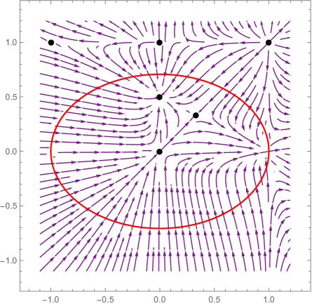
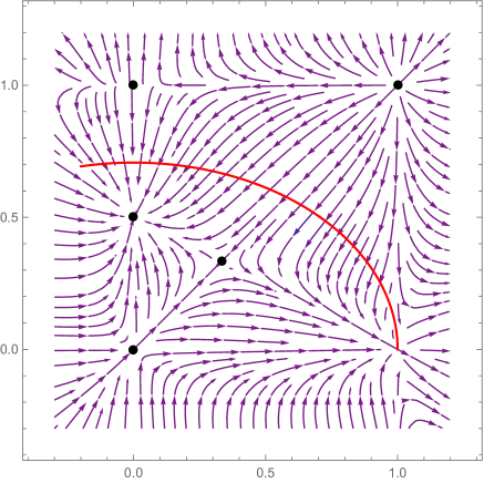
Figure 1: RG flows in the $(\lambda,\tilde{\lambda})$-plane ($\lambda$-horizontal) for $k_{2}=2k_{1}$: The entire plane (left), the first quadrant (right). The region bounded by the ellipsis is the allowed region in which the signature of the metric remains Euclidean. The arrows point towards the IR.

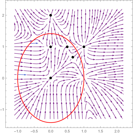
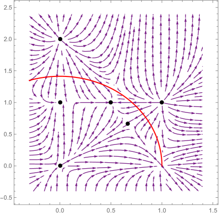
Figure 2: RG flows in the $(\lambda,\tilde{\lambda})$-plane ($\lambda$-horizontal) for $k_{1}=2k_{2}$: The entire plane (left), the first quadrant (right).

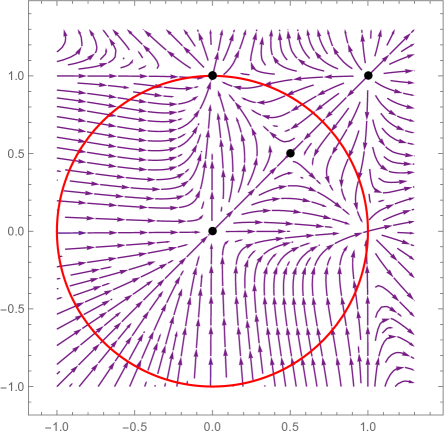
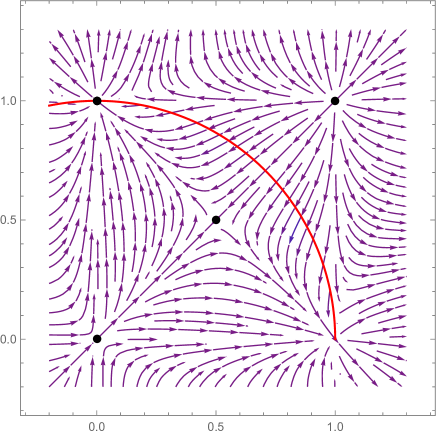
Figure 3: RG flows in the $(\lambda,\tilde{\lambda})$-plane ($\lambda$-horizontal) for $k_{1}=k_{2}$: The entire plane (left), the first quadrant (right).

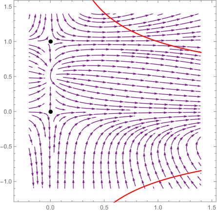
Figure 4: RG flows in the $(\zeta,\tilde{\lambda})$-plane ($\zeta$-horizontal) for the non-Abelian T-dual limit.

5 Discussion and future directions

It is a rare and remarkable occasion when one is able to derive exact results in a Quantum Field Theory (QFT) in any number of dimensions. In certain cases, this may be achieved in conjunction with some hidden symmetry, usually non-perturbative in nature, which the theory possesses. Such an example is the maximally supersymmetric gauge theory in 4-dimensions, i.e. ${\cal N}=4$ SYM, where integrability is the symmetry playing the instrumental role.

Recently, an effective and rather effortless method was developed in order to obtain exact results in certain two-dimensional QFTs. The theories under consideration are conformal field theories of the WZW type perturbed by current bilinear operators. The method relies on the construction of the corresponding all-loop effective actions for these theories [1, 2, 3]. One then uses these effective actions to determine certain non-perturbative symmetries in the space of couplings. Making the plausible assumption that the symmetries of the action are inherited by the observables of the theory, one uses low-order perturbation theory, as well as the non-perturbative symmetries in order to derive exact expressions for the observables. This programme was initiated and implemented in a series of papers mentioned in detail in the introduction in which exact expressions were obtained for the $\beta$-functions, for the anomalous dimensions of current and primary operators, as well as for the 3-point correlators involving currents and/or primary operators. We note in passing that many of the examples considered are also integrable, although this property has not been essentially in the aforementioned calculations.

In this work we continue this line of research by considering a general class of models whose UV Lagrangian is the sum of two WZW models at different levels. The perturbations driving the theory off conformality consist of current bilinears involving currents belonging to both the same and different CFTs. The all-loop effective action of these models and the corresponding equations of motion were constructed in section 2. In general these models depend on four general coupling matrices. In section 3 and for simplicity, we consider a consistent truncation of the theory in which only two of the couplings, $\lambda$ and $\tilde{\lambda}$, are present. Firstly, we identify a non-perturbative symmetry in the space of couplings $\lambda$ and $\tilde{\lambda}$. Subsequently, we proved that the theory is classically integrable by finding the appropriate Lax connection. In the same section, we also consider non-Abelian T-duality type limits for the case of the models with two couplings. We then proceeded in section 4 to derive the exact in the couplings $\beta$-functions of our model. To this end we evaluate the determinant of the matrix driving the fluctuations around a classical configuration that solves the equations of motion. The expressions for the $\beta$-functions of our model enjoy the aforementioned non-perturbative symmetry. The RG flow equations have a rich structure which also depends on the relative value of the WZW levels $k_{1}$ and $k_{2}$. Subsequently, we determine the fixed points of the flow and the nature of the corresponding CFTs in most of the cases. For the cases $k_{1}>k_{2}$ and $k_{2}>k_{1}$ there is always a fixed point, in the allowed range of the space of couplings, that is an IR attractor. This is not the case for $k_{1}=k_{2}$ where all fixed points have both relevant and irrelevant directions. Lets us also mention that our models provide concrete realisations of integrable flows between exact CFTs.

A number of open questions remain to be addressed. Firstly, it would be interesting to determine the exact nature of the CFTs in the cases not done in the present work. Secondly, one could compute the anomalous dimensions of current operators, as well as that of primary operators along the lines of [11, 12, 13, 15, 18, 4] starting with the two -coupling model of section 3. Furthermore, the exact $C$-function of the models could be calculated as was done in [18] for simpler cases. We expect that these computations will be technically quite challenging since the two coupling will both enter non-trivially in the various expressions as we have seen in the expressions for the $\beta$-functions.

Another direction would be to study the case where all four couplings are in play by determining the RG equations and identifying their fixed points. Compared to the two coupling case, we expect an even richer structure of the RG equations to be unveiled. In addition, one could search for integrability in the four coupling case. Finally, although it seems a formidable task, one could try to embed our models to solutions of type-IIB or type-IIA supergravity.

References

• [1] K. Sfetsos, Integrable interpolations: From exact CFTs to non-Abelian T-duals, Nucl. Phys. B880 (2014) 225, arXiv:1312.4560 [hep-th].
• [2] G. Georgiou and K. Sfetsos, A new class of integrable deformations of CFTs, JHEP 1703 (2017) 083, arXiv:1612.05012 [hep-th].
• [3] G. Georgiou and K. Sfetsos, Integrable flows between exact CFTs,
JHEP 1711, 078 (2017), arXiv:1707.05149 [hep-th].
• [4] G. Georgiou, K. Sfetsos and K. Siampos, Double and cyclic $\lambda$-deformations and their canonical equivalents, Phys. Lett. B771, 576 (2017), arXiv:1704.07834 [hep-th].
• [5] G. Itsios, K. Sfetsos and K. Siampos, The all-loop non-Abelian Thirring model and its RG flow, Phys. Lett.  B733 (2014) 265, arXiv:1404.3748 [hep-th].
• [6] K. Sfetsos and K. Siampos, Gauged WZW-type theories and the all-loop anisotropic non-Abelian Thirring model, Nucl. Phys. B885 (2014) 583, arXiv:1405.7803 [hep-th].
• [7] D. Kutasov, String Theory and the Nonabelian Thirring Model,
Phys. Lett. B227 (1989) 68.
• [8] B. Gerganov, A. LeClair and M. Moriconi, On the beta function for anisotropic current interactions in 2-D, Phys. Rev. Lett. 86 (2001) 4753, hep-th/0011189.
• [9] A. LeClair, Chiral stabilization of the renormalization group for flavor and color anisotropic current interactions, Phys. Lett. B519 (2001) 183, hep-th/0105092.
• [10] C. Appadu and T.J. Hollowood, Beta function of k deformed ${\text{A}dS}_{5}\times S^{5}$ string theory, JHEP 1511 (2015) 095, arXiv:1507.05420 [hep-th].
• [11] G. Georgiou, K. Sfetsos and K. Siampos, All-loop anomalous dimensions in integrable $\lambda$-deformed $\sigma$-models, Nucl. Phys.  B901 (2015) 40, arXiv:1509.02946 [hep-th].
• [12] G. Georgiou, K. Sfetsos and K. Siampos, All-loop correlators of integrable $\lambda$-deformed $\sigma$-models, Nucl. Phys. B909 (2016) 360, 1604.08212 [hep-th].
• [13] G. Georgiou, K. Sfetsos and K. Siampos, $\lambda$-deformations of left-right asymmetric CFTs, Nucl. Phys. B914 (2017) 623, arXiv:1610.05314 [hep-th].
• [14] D. Kutasov, Duality Off the Critical Point in Two-dimensional Systems With Nonabelian Symmetries, Phys. Lett. B233 (1989) 369.
• [15] G. Georgiou, E. Sagkrioti, K. Sfetsos and K. Siampos, Quantum aspects of doubly deformed CFTs, Nucl. Phys. B919 (2017) 504, arXiv:1703.00462 [hep-th].
• [16] E. Sagkrioti, K. Sfetsos and K. Siampos, RG flows for $\lambda$-deformed CFTs,
Nucl. Phys. B930 (2018) 499, arXiv:1801.10174 [hep-th].
• [17] A.B. Zamolodchikov, Irreversibility of the Flux of the Renormalization Group in a 2D Field Theory, JETP Lett. 43 (1986) 730.
• [18] G. Georgiou, P. Panopoulos, E. Sagkrioti, K. Sfetsos, K. Siampos, The exact C-function in integrable $\lambda$-deformed theories,
Phys. Lett. B782 (2018) 613-18, arXiv:1805.03731 [hep-th].
• [19] T.J. Hollowood, J.L. Miramontes and D.M. Schmidtt, Integrable Deformations of Strings on Symmetric Spaces, JHEP 1411 (2014) 009, arXiv:1407.2840 [hep-th].
• [20] T.J. Hollowood, J.L. Miramontes and D. Schmidtt, An Integrable Deformation of the $AdS_{5}\times S^{5}$ Superstring, J. Phys. A47 (2014) 49, 495402, arXiv:1409.1538 [hep-th].
• [21] K. Sfetsos and K. Siampos, Integrable deformations of the $G_{k_{1}}\times G_{k_{2}}/G_{k_{1}+k_{2}}$ coset CFTs, Nucl. Phys. B927, 124 (2018), arXiv:1710.02515 [hep-th].
• [22] G. Itsios, K. Sfetsos, K. Siampos and A. Torrielli, The classical Yang-Baxter equation and the associated Yangian symmetry of gauged WZW-type theories, Nucl. Phys. B889 (2014) 64, arXiv:1409.0554 [hep-th].
• [23] J. Balog, P. Forgacs, Z. Horvath and L. Palla, A New family of $SU(2)$ symmetric integrable sigma models, Phys. Lett. B324 (1994) 403, hep-th/9307030.
• [24] K. Sfetsos and K. Siampos, The anisotropic $\lambda$-deformed $SU(2)$ model is integrable, Phys. Lett. B743 (2015) 160, arXiv:1412.5181 [hep-th].
• [25] K. Sfetsos, K. Siampos and D.C. Thompson, Generalised integrable $\lambda$- and $\eta$-deformations and their relation, Nucl. Phys. B899 (2015) 489, arXiv:1506.05784 [hep-th].
• [26] K. Sfetsos and D.C. Thompson, Spacetimes for $\lambda$-deformations, JHEP 1412 (2014) 164, arXiv:1410.1886 [hep-th].
• [27] S. Demulder, K. Sfetsos and D.C. Thompson, Integrable $\lambda$-deformations: Squashing Coset CFTs and $AdS_{5}\times S^{5}$, JHEP 07 (2015) 019, arXiv:1504.02781 [hep-th].
• [28] R. Borsato, A. A. Tseytlin and L. Wulff, Supergravity background of $\lambda$-deformed model for AdS${}_{2}\times$ S2 supercoset, Nucl. Phys. B905 (2016) 264, arXiv:1601.08192 [hep-th].
• [29] Y. Chervonyi and O. Lunin, Supergravity background of the $\lambda$-deformed $\text{AdS}_{3}\times S^{3}$ supercoset, Nucl. Phys. B910 (2016) 685, arXiv:1606.00394 [hep-th].
• [30] C. Klimčík and P. Ševera, Dual non-Abelian duality and the Drinfeld double,
Phys. Lett. B351 (1995) 455, hep-th/9502122.
• [31] K. Sfetsos, Duality invariant class of two-dimensional field theories, Nucl. Phys. B561 (1999) 316, [hep-th/9904188].
• [32] B. Vicedo, Deformed integrable $\sigma$-models, classical $R$-matrices and classical exchange algebra on Drinfel’d doubles, J. Phys. A: Math. Theor. 48 (2015) 355203, arXiv:1504.06303 [hep-th].
• [33] B. Hoare and A.A. Tseytlin, On integrable deformations of superstring sigma models related to $AdS_{n}\times S^{n}$ supercosets, Nucl. Phys. B897 (2015) 448, arXiv:1504.07213 [hep-th].
• [34] C. Klimčík, $\eta$ and $\lambda$ deformations as ${\cal E}$-models, Nucl. Phys. B900 (2015) 259, arXiv:1508.05832 [hep-th].
• [35] C. Klimčík, Poisson–Lie T-duals of the bi-Yang–Baxter models, Phys. Lett. B760 (2016) 345, arXiv:1606.03016 [hep-th].
• [36] B. Hoare and F.K. Seibold, Poisson-Lie duals of the $\eta$-deformed $\mathrm{AdS}_{2}\times\mathrm{S}^{2}\times\mathrm{T}^{6}$ superstring, JHEP 1808 (2018) 107, arXiv:1807.04608 [hep-th].
• [37] C. Klimčík, YB sigma models and dS/AdS T-duality, JHEP 0212 (2002) 051, hep-th/0210095.
• [38] C. Klimčík, On integrability of the YB sigma-model, J. Math. Phys. 50 (2009) 043508, arXiv:0802.3518 [hep-th].
• [39] C. Klimčík, Integrability of the bi-Yang–Baxter sigma-model, Letters in Mathematical Physics 104 (2014) 1095, arXiv:1402.2105 [math-ph].
• [40] F. Delduc, M. Magro and B. Vicedo, On classical $q$-deformations of integrable sigma-models, JHEP 1311 (2013) 192, arXiv:1308.3581 [hep-th].
• [41] F. Delduc, M. Magro and B. Vicedo, An integrable deformation of the $AdS_{5}\times S^{5}$ superstring action, Phys. Rev. Lett. 112, 051601, arXiv:1309.5850 [hep-th].
• [42] G. Arutyunov, R. Borsato and S. Frolov, S-matrix for strings on $\eta$-deformed $AdS_{5}\times S^{5}$, JHEP 1404 (2014) 002, arXiv:1312.3542 [hep-th].
• [43] O. Lunin and W. Tian, Scalar fields on $\lambda$-deformed cosets, arXiv:1808.02971 [hep-th].
• [44] D.M. Schmidtt, Integrable Lambda Models And Chern-Simons Theories, JHEP 1705 (2017) 012, arXiv:1701.04138 [hep-th] and Lambda Models From Chern-Simons Theories, arXiv:1808.05994 [hep-th].
• [45] S. Driezen, A. Sevrin and D. C. Thompson, D-branes in $\lambda$-deformations, arXiv:1806.10712 [hep-th].
• [46] G. Itsios, C. Nunez, K. Sfetsos and D.C. Thompson, Non-Abelian T-duality and the AdS/CFT correspondence:new N=1 backgrounds, Nucl. Phys. B873 (2013) 1, arXiv:1301.6755 [hep-th].
• [47] T. Curtright and C. K. Zachos, Currents, charges, and canonical structure of pseudodual chiral models, Phys. Rev. D49 (1994) 5408, hep-th/9401006.
• [48] Y. Lozano, Non-Abelian duality and canonical transformations, Phys. Lett. B355 (1995) 165, hep-th/9503045.
• [49] K. Sfetsos, Non-Abelian duality, parafermions and supersymmetry, Phys. Rev. D54 (1996) 1682, hep-th/9602179.
• [50] N. Mohammedi, On the geometry of classically integrable two-dimensional non-linear sigma models, Nucl. Phys. B839 (2010) 420, arXiv:0806.0550 [hep-th].
• [51] G. Ecker and J. Honerkamp, Application of invariant renormalization to the nonlinear chiral invariant pion Lagrangian in the one-loop approximation, Nucl. Phys. B35 (1971) 481. J. Honerkamp, Chiral multiloops, Nucl. Phys. B36 (1972) 130.
• [52] D. Friedan, Nonlinear Models in Two Epsilon Dimensions, Phys. Rev. Lett. 45 (1980) 1057 and Nonlinear Models in Two + Epsilon Dimensions, Annals Phys.  163 (1985) 318.
• [53] T. L. Curtright and C. K. Zachos, Geometry, Topology and Supersymmetry in Nonlinear Models, Phys. Rev. Lett.  53 (1984) 1799. E. Braaten, T. L. Curtright and C. K. Zachos, Torsion and Geometrostasis in Nonlinear Sigma Models, Nucl. Phys. B260 (1985) 630. B.E. Fridling and A.E.M.van de Ven, Renormalization of Generalized Two-dimensional Nonlinear $\sigma$-Models, Nucl. Phys. B268 (1986) 719.