Confinement of Brownian Polymers under Geometric Area Tilts

Abstract.

We consider tightness for families of non-colliding Brownian bridges above a hard wall, which are subject to geometrically growing self-potentials of tilted area type. The model is introduced in order to mimic level lines of $2+1$ discrete Solid-On-Solid random interfaces above a hard wall.

1. Brownian polymers under geometric area tilts.

1.1. Introduction

Ensembles of non-intersecting random lines, both in the discrete and continuous setups, as well as their scaling limits as the linear size of the system grows, play a significant role in the probabilistic analysis of various problems in random matrices, interacting particle systems and effective interface models; see e.g. [10, 17, 22, 8, 2, 1, 18, 24, 7, 9] and references therein.

A salient feature of these ensembles is that the unconditional reference distribution of the individual random lines is assumed to be the same for all the random lines in a stack. The ensuing exchangeability paves the way for an application of Karlin-McGregor type formulas, and gives rise to various determinantal structures.

In this paper, we introduce a model consisting of an unbounded number of non-intersecting Brownian bridges, above a hard wall and subject to geometrically increasing area tilts.

Thus, in our model reference statistics of individual lines depends on their serial numbers - there is a stronger pressure towards the wall on paths further down the stack. The main result of the paper is that the ensemble in question does not blow up as the number of bridges grows to infinity. There is a longer program to attend to: In subsequent works we shall describe the limiting (infinite) line ensemble and try to derive appropriate scaling limits from tilted random walks and, eventually, from level lines of discrete random interfaces. Indeed, the main motivation comes from the study of the fluctuations of level lines in the random surface separating low-temperature phases in the solid-on-solid (SOS) approximation of the 3D Ising model. Before describing our model and main results, let us give more details about the context where the model naturally arises, we refer to [4, 5, 15, 19], for further information.

1.2. Level lines of SOS interfaces above a hard wall.

Given a large integer $L$, consider the square box $\Lambda_{L}$ of side $2L$ in $\mathbb{Z}^{2}$, centered at the origin. The $(2+1)$-dimensional SOS Gibbs measure on $\Lambda_{L}$ with zero boundary conditions is the distribution $\mu_{L}$ over integer height functions $\varphi:\Lambda_{L}\mapsto\mathbb{Z}$, such that the probability of each given configuration $\varphi$ is proportional to

$$\exp\left(-\beta\sum_{x\sim y}|\varphi(x)-\varphi(y)|\right),$$

where $\beta>0$ denotes the inverse temperature, and the sum extends over all pairs of neighbouring sites in $\mathbb{Z}^{2}$, with the boundary constraint $\varphi(y)=0$ for all $y\in\mathbb{Z}^{2}\setminus\Lambda_{L}$. When $\beta$ is larger than some fixed constant, which we assume throughout this discussion, the surface $\varphi$ with distribution $\mu_{L}$ is typically flat around height zero with local upward and downward fluctuations of depth $h$ with density roughly proportional to $e^{-4\beta h}$ for all $h\in\mathbb{N}$. If the surface is constrained to stay above a hard wall, that is $\mu_{L}$ is conditioned on the event $\{\varphi(x)\geq 0,x\in\Lambda_{L}\}$, then it is well known that the wall pushes the surface globally to a height

$$H(L)\sim\frac{1}{4\beta}\log L,$$

see [3, 4]. This phenomenon, known as entropic repulsion, is heuristically explained as follows: a global shift of the surface from height $h-1$ to height $h$ provides room for downward fluctuations of depth $h$, which gives a bulk entropic gain of order $|\Lambda_{L}|e^{-4\beta h}$, while forcing an energy loss proportional to the size of the boundary $|\partial\Lambda_{L}|$; the surface then stabilises when energy and entropy balance out, that is when $h$ equals $H(L)\sim\frac{1}{4\beta}\log L$.

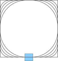
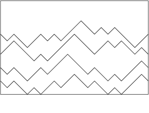
Figure 1. Left: sketch of the top four nested limiting lines $\mathcal{L}_{h}$, $h=1,\dots,4$ within the square $Q=[-1,1]^{2}$. The shaded region contains only macroscopically flat portions of the lines. Right: fluctuations of the lines on a scale of smaller order obtained by zooming in the shaded region.

In [5] it was shown that at equilibrium, the SOS surface above the wall is characterized by a uniquely defined ensemble $\Gamma$, consisting of the nested macroscopic contours (closed loops in the dual lattice, within $\Lambda_{L}$)

$$\Gamma=\{\gamma_{1}\subseteq\dots\subseteq\gamma_{n}\subseteq\partial\Lambda_{L}\},$$

where $n=H(L)$, with the interpretation that $\gamma_{h}$ is the $(H(L)-h)$-th level line of the surface, so that $\varphi$ grows from at most $H(L)-h$ to at least $H(L)-h+1$ upon crossing $\gamma_{h}$. Moreover, it was shown that the contour ensemble satisfies a law of large numbers, that is if the box $\Lambda_{L}$ is rescaled to the square $Q=[-1,1]^{2}$, then when $L\to\infty$, the contours concentrate around a limiting shape consisting of infinitely many nested loops $\mathcal{L}_{1}\subseteq\mathcal{L}_{2}\subseteq\cdots\subseteq\partial Q$. The loops $\mathcal{L}_{h}$ can be identified via constrained Wulff variational principles: each single $\mathcal{L}_{h}$ is a rescaled Wulff plaquette such as that already studied in the context of $2D$ Ising model [21]. A related low temperature SOS-type model which, under appropriate rescaling, features a stack of identical Wulff plaquettes was studied in [12].

In our case nested loops $\mathcal{L}_{h}$ are strictly ordered by inclusion. However, apart from round pieces in the neighbourhood of the four corners of $Q$ (which are different for different plaquettes $\mathcal{L}_{h}$-s), all $\mathcal{L}_{h}$, $h\geq 1$, contain flat pieces, where they coincide with the boundary of $Q$; see Figure 1. In particular, there exists $u\in(0,1)$ (with $u=u(\beta)\to 1$ as $\beta\to\infty$) such that the portion $I_{u}=[-u,u]\times\{-1\}\subset\partial Q$ of the bottom side of $Q$ is contained in all loops $\mathcal{L}_{1},\mathcal{L}_{2},\dots$

To study fluctuations of the level lines of the surface it is then necessary to zoom in the shaded region from Figure 1 and understand at what rate the contour ensemble $\Gamma$ converges to the flat limit there as $L\to\infty$. In this direction, it was shown in [5] that the maximal distance of the top contour $\gamma_{1}$ from the bottom boundary of $Q$ is typically of order $L^{\frac{1}{3}+o(1)}$ and that fluctuations of that order appear on every subinterval of length $L^{\frac{2}{3}+o(1)}$, where $o(1)$ denotes a quantity vanishing as $L\to\infty$.

In a first attempt, we may approximate the $n$ paths in the above mentioned region by $n$ ordered height functions $\Psi=\{\psi_{1},\dots,\psi_{n}\}$ with free endpoints, where $\psi_{i}:[-L,L]\mapsto\mathbb{N}$, $\psi_{i}(x)\geq\psi_{i+1}(x)\geq 0$ for all $x$; see Figure 1. As discussed in [5], contour analysis based on cluster expansion techniques shows that the statistical weight of a configuration $\Psi$ of such lines is essentially given by

$$\exp\left(-\sum_{i=1}^{n}\left[\beta E(\psi_{i})+\frac{a\lambda^{i}}{L}\,A(\psi_{i})\right]\right).$$ (1.1)

Here $E(\psi_{i})=\sum_{x}|\psi_{i}(x+1)-\psi_{i}(x)|$ denotes the energy cost of the $i$-th path, $a=a(\beta)>0$ and $\lambda=\lambda(\beta)>1$ are suitable constants, $A(\psi_{i})=\sum_{x}\psi_{i}(x)$ is the area between the path $\psi_{i}$ and the bottom layer at height zero, while the term $a\lambda^{i}$ quantifies the entropic repulsion felt by the $i$-th path, which in these new coordinates becomes an effective attraction to the bottom. In agreement with their mutual order, the attraction felt by the $i$-th path is stronger than the attraction felt by the $(i-1)$-th path. It should be remarked that in the description (1.1) we are completely neglecting some nontrivial interaction terms between the paths $\psi_{i}$, which account for possible weak attractive and repulsive potentials along the polymer boundaries (pinning effects); while these terms should be indeed irrelevant if $\beta$ is sufficiently large, showing that this is actually the case can be a challenging problem; see [5, 13].

1.3. Ferrari-Spohn and Dyson-Ferrari-Spohn diffusions.

The expression (1.1) describes a growing number of ordered random walks above a wall with geometrically growing area tilts. The case of a single walk $n=1$ is an effective random walk model for the critical pre-wetting problem in the $2D$ Ising model; see [21, 23]. This case was recently studied in [14], where it was shown in particular that if $\ell=L^{\frac{2}{3}}$, then the rescaled path

$$x(t)=\frac{1}{\sqrt{\ell}}\,\psi_{1}(t\ell)\,,\qquad t\in\mathbb{R},$$ (1.2)

as $L\to\infty$ converges weakly to the stationary Ferrari-Spohn diffusion, namely the reversible diffusion process on $\mathbb{R}_{+}$ with potential given by the logarithm of the Airy function, which was first introduced in [11]. On the other hand, for fixed $n$, and for $\lambda=1$, the ensemble of random lines described by (1.1) has been analysed in [16], where it is shown that the vector of rescaled trajectories

$$\underline{x}(t)=\frac{1}{\sqrt{\ell}}\,(\psi_{1}(t\ell),\dots,\psi_{n}(t\ell))\,,\qquad t\in\mathbb{R},$$

converges weakly to the stationary Dyson-Ferrari-Spohn diffusion, that is the determinantal process on $\mathbb{R}_{+}^{n}$ corresponding to $n$ non-intersecting Ferrari-Spohn diffusions.

1.4. The model and the result.

The case of $n$ ordered random walks with $n$ growing with $L$ (e.g.  $n\propto\log L$ as in the original setting of SOS level lines) and $\lambda>1$ will be the subject of a separate paper. At this stage it is even unclear whether, under the Ferari-Spohn scaling (1.2), such ensemble has a meaningful limit. This is precisely the issue which we explore here. For simplicity, and in order to stress main quantitative features of the phenomenon under consideration, we shall consider a continuous analogue of the above model, where discrete random walk paths are replaced by Brownian motion paths. The corresponding model then becomes the ensemble of non-intersecting Brownian motions $X_{i}\geq X_{i+1}\geq 0$, $i=1,\dots,n$ on $[-T,T]$, for some $T>0$, with free endpoints, deformed by the statistical weight

$$\exp\left(-\sum_{i=1}^{n}a\lambda^{i}A(X_{i})\right)$$ (1.3)

where $a>0,\lambda>1$ and $A(X_{i})=\int_{-T}^{T}X_{i}(s)ds$.

If $n=1$ then taking $T\to\infty$ one recovers (without further rescaling) the stationary Ferrari-Spohn diffusion. Similarly, if $n$ is fixed and $\lambda=1$, then $T\to\infty$ yields the stationary Dyson-Ferrari-Spohn diffusion. The invariant measure of the latter is given by Slater determinants associated to the eigenfunctions of Airy differential operator with Dirichlet boundary condition at the origin. As $n\to\infty$ there are various (edge, bulk, $\dots$) scaling regimes, which were described on the level of the corresponding determinantal point processes in [1].

In our case; $n$ growing with $T$ and $\lambda>1$, no scaling is needed and the random line ensemble described by (1.3) will have a very different limiting behavior, and a very different weak limit which would, with appropriate modifications related to the nature of area tilts, fall into the framework of $\mathbb{N}\times\mathbb{R}$-indexed Brownian-Gibbs ensembles as developed in [8]. Indeed, it seems natural to conjecture that as $n\to\infty$ and $T\to\infty$ (regardless of the order), the process converges to a unique $\mathbb{N}\times\mathbb{R}$-indexed random line ensemble, in particular that for every $k\in\mathbb{N}$ the top $k$ lines $X_{1},\dots,X_{k}$ weakly converge to a stationary $k$-dimensional process. For the moment, guessing the precise structure of the limiting process remains an intriguing question. On the other hand, the route to proving convergence per se is, in light of the stability results we derive here, rather clear - see Remark 1 following (1.4) below. This issue will be addressed in a forthcoming separate paper.

Here we focus on deriving uniform stability properties of the system of paths associated to (1.3) as $n,T\to\infty$. Namely, we prove the following strong confinement statement about the top path $X_{1}$ (and hence about the whole stack which is sandwiched between $X_{1}$ and the wall): Fix $\varepsilon>0$ and let $\left[\cdot\right]_{+}$ denote the positive part. Then expectations of curved maxima

$$\sup_{T,n}\,\mathbb{E}\left(\max_{t\in[-T,T]}\big{[}{X_{1}(t)-|t|^{\varepsilon}}]_{+}\right)<\infty,$$ (1.4)

are uniformly bounded in $T$ and $n$. See Theorem 3.1 for the precise statement.

Remark 1.

The bound (1.4) paves the way for importing techniques and ideas developed in [8], in particular for deriving appropriate adjustments of Proposition 3.5 and of the tightness arguments employed for the proof of Proposition 3.6 of the latter work. Indeed, fix $k\in\mathbb{N}$ and an interval $(-a,a)$ and, for $n>k$ and $T>a$, consider top $k$ paths $X_{1},\dots,X_{k}$ of the line ensemble of $n$ non-intersecting Brownian motions on $[-T,T]$ under geometric area tilts (1.3). But then (1.4) means two things: First of all, by Brownian scaling and stochastic domination - see Subsections 1.5.1 and 1.5.3 below, the height of the $(k+1)$-st path $X_{k+1}$ is, uniformly in $n$ and $T$, under control in the sense that it sits below a random integrable shift of the appropriate rescaling of $t^{\epsilon}$. Next, given a realization of $X_{k+1}$, the top paths $X_{1},\dots,X_{k}$ could be, by Brownian-Gibbs property, resampled according to Brownian bridge measures modified by exponential weights (1.3). But these weights are, by the very same (1.4), also subject to a uniform control. Resampling with respect to reference Brownian bridge measures (that is with zero area tilts) is precisely the procedure employed for Airy line ensembles in [8]. As a result many probabilistic estimates could be, up to uniformly bounded corrections, inherited from the resampling estimates developed in [8].

We proceed with precise notation for the polymer measures we study here.

1.4.1. Notation for underlying Brownian motion and Brownian bridges.

In the sequel we shall use the same notation for path measures of underlying Brownian motion and Brownian bridges and for expectations with respect to these path measures. For $S<T$ and $x\in\mathbb{R}$, let ${\mathbf{P}}^{x}_{S,T}$ be the path measure of the Brownian motion $X$ on $[S,T]$ which starts at $x$ at time $S$; $X(S)=x$. We can record ${\mathbf{P}}^{x}_{S,T}$ as follows:

$${\mathbf{P}}^{x}_{S,T}\left(F(X)\right)=\int{\mathbf{B}}^{x,y}_{S,T}\left(F(X)\right){\rm d}y$$ (1.5)

where ${\mathbf{B}}^{x,y}_{S,T}$ the unnormalized path measure of the Brownian bridge $X$ on $[S,T]$ which starts at $x$ at time $S$ and ends at $y$ at time $T$; $X(S)=x,\,X(T)=y$. In this notation

$${\mathbf{B}}^{x,y}_{S,T}(1)=\tfrac{1}{\sqrt{2\pi(T-S)}}\,{\rm e}^{-\frac{(y-x)^{2}}{2(T-S)}}.$$

For an $n$-tuple $\underline{x}\in\mathbb{R}^{n}$, set

$${\mathbf{P}}^{\underline{x}}_{S,T}={\mathbf{P}}^{x_{1}}_{S,T}\otimes{\mathbf{P}}^{x_{2}}_{S,T}\otimes\cdots\otimes{\mathbf{P}}^{x_{n}}_{S,T}.$$

Similarly for $n$-tuples $\underline{x},\underline{y}\in\mathbb{R}^{n}$, set

$${\mathbf{B}}^{\underline{x},\underline{y}}_{S,T}={\mathbf{B}}^{x_{1},y_{1}}_{S,T}\otimes{\mathbf{B}}^{x_{2},y_{2}}_{S,T}\otimes\cdots\otimes{\mathbf{B}}^{x_{n},y_{n}}_{S,T}.$$

For symmetric intervals $S=-T$ we shall employ a reduced notation ${\mathbf{P}}^{\underline{x}}_{T}$, ${\mathbf{B}}^{\underline{x},\underline{y}}_{T}$ and so on.

1.4.2. Partition functions and polymer measures with geometric area tilts.

Given a function $h$, the signed $h$-area under the trajectory of $X$ is defined as

$$\mathcal{A}_{S,T}^{h}\left(X\right)=\int_{S}^{T}h(t)X(t){\rm d}t.$$ (1.6)

We shall drop the superscript if $h\equiv 1$ and use $\mathcal{A}_{S,T}\left(X\right)$ accordingly. For $n\in\mathbb{N}$ define

$$\mathbb{A}_{n}^{+}=\{\underline{x}\in\mathbb{R}^{n}\,:\,x_{1}>\dots>x_{n}>0\}.$$ (1.7)

Polymer measures which we consider in the sequel are always concentrated on the set $\Omega^{+}_{n,S,T}$ of $n$-tuples $\underline{X}$,

$$\Omega^{+}_{n,S,T}=\left\{\underline{X}~{}:~{}\underline{X}(t)\in\mathbb{A}_{n}^{+}\ \ \forall\,t\in[S,T]\right\}$$ (1.8)

Following our convention we shall write $\Omega^{+}_{n,T}=\Omega^{+}_{n,-T,T}$.

Given $n\geq 1$, $a>0$ and $\lambda>1$ consider now the partition functions

$$\begin{split}Z_{n,T}^{\underline{x},\underline{y}}(a,\lambda)&\stackrel{{\scriptstyle\Delta}}{{=}}{\mathbf{B}}^{\underline{x},\underline{y}}_{T}\left(\mathbbm{1}_{\Omega_{n,T}^{+}}{\rm e}^{-\sum_{1}^{n}a\lambda^{i-1}\mathcal{A}_{T}(X_{i})}\right)\\ &{\rm and}\\ {\mathcal{Z}}_{n,T}(a,\lambda)&\stackrel{{\scriptstyle\Delta}}{{=}}\int_{\mathbb{A}_{n}^{+}}\int_{\mathbb{A}_{n}^{+}}Z_{n,T}^{\underline{x},\underline{y}}(a,\lambda){\rm d}\underline{x}{\rm d}\underline{y}.\end{split}$$ (1.9)

Partition functions ${\mathcal{Z}}_{n,T}(a,\lambda)$ give rise to polymer measures $\mathbb{P}_{n,T}\left[\cdot~{}|a,\lambda\right]$. with geometric area tilts $\rho_{i}\equiv a\lambda^{i-1}$. Namely,

$$\mathbb{P}_{n,T}\left[F(\underline{X})~{}|a,\lambda\right]\ \stackrel{{\scriptstyle\Delta}}{{=}}\frac{1}{{\mathcal{Z}}_{n,T}(a,\lambda)}\int_{\mathbb{A}_{n}^{+}}\int_{\mathbb{A}_{n}^{+}}{\mathbf{B}}^{\underline{x},\underline{y}}_{T}\left(F(\underline{X})\mathbbm{1}_{\Omega_{n,T}^{+}}{\rm e}^{-\sum_{1}^{n}\mathcal{A}_{T}^{\rho_{i}}(X_{i})}\right){\rm d}\underline{x}{\rm d}\underline{y}$$ (1.10)

1.4.3. Main result.

The main result of this note could be formulated as follows:

Theorem 1.1.

Let $\mathcal{P}_{n,T}\left[\cdot~{}|a,\lambda\right]$ be the (one-dimensional) distribution of the position of the top path $X_{1}(0)$ under $\mathbb{P}_{n,T}\left[\cdot~{}|a,\lambda\right]$. That is

$$\mathcal{P}_{n,T}\left[f({X})~{}|a,\lambda\right]=\mathbb{P}_{n,T}\left[f(X_{1}(0))~{}|a,\lambda\right],$$

for bounded measurable $f:\mathbb{R}\mapsto\mathbb{R}$. Then for any fixed $a>0$ and $\lambda>1$ the family of one-dimensional distributions $\left\{\mathcal{P}_{n,T}\left[\cdot~{}|a,\lambda\right]\right\}_{n,T}$ is tight. In other words the top path does not fly away as the number of polymers and the length of their horizontal span grow.

Theorem 1.1 is an immediate consequence of a much stronger confinement statement for the curved maximum of the whole path - see Theorem 3.1 below.

1.5. Structure of the proof.

The proof is built upon a recursion which relies on the Brownian scaling and on stochastic domination for (a more general class of) polymers with area tilts:

1.5.1. Brownian scaling.

Consider the following mapping of an $n$-tuple $\underline{X}$ of paths on an interval $[-\lambda^{2/3}T,\lambda^{2/3}T]$ to $n$-tuple $\underline{Y}$ of paths on $[-T,T]$:

$$\underline{Y}(\cdot)=\frac{1}{\lambda^{1/3}}\underline{X}(\lambda^{2/3}\cdot).$$ (1.11)

The next lemma states that if $\underline{Y}$ is related to $\underline{X}$ via (1.11), then $\underline{Y}$ has distribution $\mathbb{P}_{n,T}\left[\cdot~{}|a\lambda,\lambda\right]$ if and only if $\underline{X}$ has distribution $\mathbb{P}_{n,T\lambda^{2/3}}\left[\cdot~{}|a,\lambda\right]$.

Lemma 1.1.

For all $n,T$, $a,\lambda$, and $\underline{x},\underline{y}$

$$Z_{n,T\lambda^{2/3}}^{\underline{x},\underline{y}}(a,\lambda)=\lambda^{-\frac{n}{3}}Z_{n,T}^{\lambda^{-1/3}\underline{x},\lambda^{-1/3}\underline{y}}(a\lambda,\lambda).$$ (1.12)

Furthermore, for any bounded measurable function $F$ on $\Omega_{n,T}^{+}$,

$$\mathbb{P}_{n,T}\left[F(\underline{X})~{}|a\lambda,\lambda\right]=\mathbb{P}_{n,T\lambda^{2/3}}\left[F(\underline{X}^{(\lambda^{2/3})})~{}|a,\lambda\right],$$ (1.13)

where $\underline{X}^{(\lambda^{2/3})}=\frac{1}{\lambda^{1/3}}\underline{X}(\lambda^{2/3}\cdot)$.

Proof.

For any $\gamma>0$, consider the map $\Omega_{n,\gamma T}^{+}\mapsto\Omega_{n,T}^{+}$ defined by

$$\underline{X}^{(\gamma)}(t)=\gamma^{-\frac{1}{2}}\underline{X}(\gamma t)\,,\qquad t\in[-T,T].$$

The normalized Brownian bridge ensemble

$$\Gamma^{\underline{x},\underline{y}}_{T}=\frac{{\mathbf{B}}^{\underline{x},\underline{y}}_{T}}{{\mathbf{B}}^{\underline{x},\underline{y}}_{T}(1)},$$

has the Brownian scaling property:

$$\Gamma^{\underline{x},\underline{y}}_{\gamma T}[G(\underline{X}^{(\gamma)})]=\Gamma^{\gamma^{-\frac{1}{2}}\underline{x},\gamma^{-\frac{1}{2}}\underline{y}}_{T}[G(\underline{X})]\,,\qquad\gamma>0,$$ (1.14)

where $G$ is any bounded measurable function on $\Omega_{n,T}^{+}$. We apply (1.14) with

$$G(\underline{X})=\mathbbm{1}_{\Omega_{n,T}^{+}}(\underline{X})\,{\rm e}^{-\sum_{1}^{n}a\lambda^{i-1}\mathcal{A}_{T}(X_{i})},$$

and $\gamma=\lambda^{2/3}$. Since, the area under the path scales as

$$\frac{1}{\lambda}\int_{-T\lambda^{2/3}}^{T\lambda^{2/3}}X_{i}(t)dt=\int_{-T}^{T}\frac{X_{i}(t\lambda^{2/3})}{\lambda^{1/3}}dt,$$

this yields (1.12). The proof of (1.13) is similar, with

$$G(\underline{X})=F(\underline{X})\mathbbm{1}_{\Omega_{n,T}^{+}}(\underline{X})\,{\rm e}^{-\sum_{1}^{n}a\lambda^{i-1}\mathcal{A}_{T}(X_{i})}.$$

∎

1.5.2. A general class of polymers with area tilts.

Let us say that two continuous functions $f$ and $g$ on $[-T,T]$ satisfy $f\prec g$ if $f(t)\leq g(t)$ for any $t\in[-T,T]$. By construction, if $\underline{X}\in\Omega_{n,T}^{+}$, then $0\prec X_{n}\prec X_{n-1}\prec\dots\prec X_{1}$. For every $n\in\mathbb{N}$ and $T>0$, let us consider the following general class $\mathbb{P}_{n,T}^{\underline{x},\underline{y}}\left[\,\cdot|h_{-},h_{+},\underline{\rho}\right]$ of polymer measures which is parametrized by:

a:

Boundary conditions $\underline{x},\underline{y}\in\mathbb{A}_{n}^{+}$.

b:

Two non-negative continuous functions $h_{-}\prec h_{+}$ on $[-T,T]$, which are called the floor $h_{-}$ and the ceiling $h_{+}$.

c:

A tuple of $n$ (not necessarily ordered) positive continuous functions $\underline{\rho}=\left\{\rho_{1},\dots,\rho_{n}\right\}$ which are called area tilts.

Then, setting

$$\Omega_{n,T}^{\underline{h}}=\Omega_{n,T}^{+}\cap\left\{h_{-}\prec X_{n}\prec X_{1}\prec h_{+}\right\},$$ (1.15)

define:

$$\mathbb{P}_{n,T}^{\underline{x},\underline{y}}\left[{\rm d}\underline{X}|h_{-},h_{+},\underline{\rho}\right]\,\propto\,{\rm e}^{-\sum_{1}^{n}\mathcal{A}_{T}^{\rho_{i}}(X_{i})}\mathbbm{1}_{\Omega_{n,T}^{\underline{h}}}{\mathbf{B}}_{T}^{\underline{x},\underline{y}}\left({\rm d}\underline{X}\right).$$ (1.16)

The corresponding partition function is denoted $Z_{n,T}^{\underline{x},\underline{y}}(h_{-},h_{+},\underline{\rho})$.

There is a version of (1.16) which permits more general boundary conditions: Let $\underline{\nu}$ and $\underline{\eta}$ be $n$-tuples of functions on $\mathbb{R}_{+}$. For $\underline{x}\in\mathbb{A}_{n}^{+}$ set $\underline{\nu}(\underline{x})=\sum_{1}^{n}\nu_{i}(x_{i})$, and $\underline{\eta}(\underline{x})=\sum_{1}^{n}\eta_{i}(x_{i})$. Similarly, set $\mathcal{A}_{T}^{\underline{\rho}}(\underline{X})=\sum_{1}^{n}\mathcal{A}_{T}^{\rho_{i}}(X_{i})$. Then,

$$\mathbb{P}_{n,T}^{\underline{\nu},\underline{\eta}}\left[{\rm d}\underline{X}|h_{-},h_{+},\underline{\rho}\right]\,\propto\,\int_{\mathbb{A}_{n}^{+}}\int_{\mathbb{A}_{n}^{+}}{\rm e}^{-\mathcal{A}_{T}^{\underline{\rho}}(\underline{X})}\mathbbm{1}_{\Omega_{n,T}^{\underline{h}}}\left(\underline{X}\right){\rm e}^{-\underline{\nu}(\underline{x})}{\mathbf{B}}_{T}^{\underline{x},\underline{y}}\left({\rm d}\underline{X}\right){\rm e}^{-\underline{\eta}(\underline{y})}{\rm d}\underline{x}{\rm d}\underline{y}.$$ (1.17)

The corresponding partition function is denoted $\mathcal{Z}_{n,T}^{\underline{\eta},\underline{\nu}}(h_{-},h_{+},\underline{\rho})$. This notation could be made formally compatible with (1.9) as follows: if we define $\delta_{x}(y)=\infty\mathbbm{1}_{y\neq x}$, and, for a tuple $\underline{x}$ define the $n$-tuple $\underline{\delta}_{\underline{x}}=\left\{\delta_{x_{1}},\dots,\delta_{x_{n}}\right\}$, then $Z_{n,T}^{\underline{x},\underline{y}}(h_{-},h_{+},\underline{\rho})=\mathcal{Z}_{n,T}^{\underline{\delta}_{\underline{x}},\underline{\delta}_{\underline{y}}}(h_{-},h_{+},\underline{\rho}).$

Reduced notation. In the sequel we shall, unless this creates a confusion, employ the following reduced notation: If $\underline{\eta},\underline{\nu}$ are identically zero, we shall drop them from the notation. We refer to this as the case of free (or empty) boundary conditions. Similarly we shall drop from the notation the floor $h_{-}$ whenever $h_{-}\equiv 0$ and the ceiling $h_{+}$ whenever $h_{+}\equiv\infty$. Furthermore, we shall write $a,\lambda$ instead of $\underline{\rho}$ whenever $\underline{\rho}=\left\{a,a\lambda,\dots,a\lambda^{n-1}\right\}$. Finally we shall drop $n$ whenever talking about just one polymer, $n=1$. In this way we make new notation compatible with (1.10).

Below we shall tacitly assume that boundary conditions $\underline{\nu},\underline{\eta}$ are chosen in such a way that the corresponding polymer measures are well defined. In Appendix A this assumption will be justified for a class of boundary conditions $\underline{\nu},\underline{\eta}$, including free boundary conditions.

1.5.3. Stochastic domination.

Equip $\Omega_{n,T}^{+}$ with the partial order $\prec$, defined by

$$\underline{X}\prec\underline{Y}\;\;\text{iff}\;\;X_{i}\prec Y_{i}\,,\;\text{for all }\,i,$$

and let $\stackrel{{\scriptstyle\mathsf{FKG}}}{{\prec}}$ denote the associated notion of stochastic domination of probability measures.

Lemma 1.2.

For any $n$ and $T$, $h_{-}\prec g_{-}$, $h_{+}\prec g_{+}$, $\underline{\rho}\succ\underline{\kappa}$, the following holds. If, $\underline{x}\prec\underline{u}$ and $\underline{y}\prec\underline{v}$, then

$$\mathbb{P}_{n,T}^{\underline{x},\underline{y}}\left[\cdot|h_{-},h_{+},\underline{\rho}\right]\stackrel{{\scriptstyle\mathsf{FKG}}}{{\prec}}\mathbb{P}_{n,T}^{\underline{u},\underline{v}}\left[\cdot|g_{-},g_{+},\underline{\kappa}\right].$$ (1.18)

Moreover, for an $n$-tuple $\underline{\chi}=\left\{\chi_{1},\dots,\chi_{n}\right\}$ of smooth boundary condition let $\underline{\chi}^{\prime}$ be the $n$-tuple of corresponding first derivatives. Then,

$$\mathbb{P}_{n,T}^{\underline{\xi},\underline{\zeta}}\left[\cdot|h_{-},h_{+},\underline{\rho}\right]\stackrel{{\scriptstyle\mathsf{FKG}}}{{\prec}}\mathbb{P}_{n,T}^{\underline{\nu},\underline{\eta}}\left[\cdot|g_{-},g_{+},\underline{\kappa}\right],$$ (1.19)

whenever, $h_{-}\prec g_{-}$, $h_{+}\prec g^{+}$, $\underline{\rho}\succ\underline{\kappa}$ and, both $\underline{\xi}^{\prime}\succ\underline{\nu}^{\prime}$ and $\underline{\zeta}^{\prime}\succ\underline{\eta}^{\prime}$. In particular, (1.19) holds if $\underline{\xi}=\underline{\nu}$ and $\underline{\zeta}=\underline{\eta}$ (by approximation without any assumptions on smoothness).

The proof of Lemma 1.2 is given in Section B below.

1.5.4. A recursion.

Consider our polymer measure $\mathbb{P}_{n+1,T}\left[\cdot~{}|a,\lambda\right]$. Let us record $\underline{X}=(X_{1},\tilde{}\underline{X})$, where $\tilde{}\underline{X}=(X_{2},\dots,X_{n+1})$. It is easy to see that the conditional, on $X_{1}$, distribution of $\tilde{}\underline{X}$ is precisely $\mathbb{P}_{n,T}\left[\cdot|X_{1},a\lambda,\lambda\right]$ with ceiling $X_{1}$. By (1.19) it is stochastically dominated by $\mathbb{P}_{n,T}\left[\cdot|a\lambda,\lambda\right]$. Therefore, if $F$ is a non-decreasing function on $\Omega_{n,T}^{+}$,

$$\mathbb{E}_{n+1,T}\left[F(\tilde{\underline{X}})|a,\lambda\right]\leq\mathbb{E}_{n,T}\left[F({\underline{X}})|a\lambda,\lambda\right].$$ (1.20)

Let $f$ be a non-decreasing functional of $X_{1}$. Then, conditioning on $X_{2}$,

$$\mathbb{E}_{n+1,T}\left[f(X_{1})\,\big{|}\,X_{2}\,|\,a,\lambda\right]=\mathbb{E}_{T}\left[f(X)\big{|}\,X_{2},a\right]$$ (1.21)

is, by (1.19), a non-decreasing functional of the floor $X_{2}$. Applying (1.20) with $F(\tilde{}\underline{X})=\mathbb{E}_{T}\left[f(X)\big{|}\,X_{2},a\right]$ and then using the scaling property (1.13), this means:

$$\begin{split}\mathbb{E}_{n+1,T}\left[f(X_{1})|a,\lambda\right]&\leq\mathbb{E}_{n,T}\left[\mathbb{E}_{T}\left[f(X)\big{|}\,X_{1},a\right]\big{|}a\lambda,\lambda\right]\\ &\stackrel{{\scriptstyle\eqref{eq:BScale-11}}}{{=}}\mathbb{E}_{n,T\lambda^{2/3}}\left[\mathbb{E}_{T}\left[f(X)\big{|}\,\frac{X_{1}(\lambda^{2/3}\cdot)}{\lambda^{1/3}},a\right]\big{|}a,\lambda\right].\end{split}$$ (1.22)

Inequality (1.22) sets up the stage for various recursions which eventually lead to tightness statements like the one formulated in Theorem 1.1. In particular, a natural choice of $f(X)=\max_{t\in[-T,T]}X(t)$ in (1.22) leads to a proof of tightness (in $n$) of the maxima for each $T$ fixed, but clearly is not suitable for proving tightness uniformly in $T$. In order to prove Theorem 1.1 we introduce a kind of curved maximum, and use (1.22) to control it uniformly in $n$ and $T$. Both the usual and the curved maxima are discussed in the subsequent sections.

Remark 2.

Let us also remark that the above reasoning can be used to control the height of the $k$-th path $X_{k}$ in terms of the top path $X_{1}$. Indeed, as in (1.20) one has that $X_{k+1}$ under $\mathbb{P}_{n,T}\left[\cdot|a,\lambda\right]$ is stochastically dominated by $X_{k}$ under $\mathbb{P}_{n-1,T}\left[\cdot|a\lambda,\lambda\right]$. Iterating, it follows that $X_{k+1}$ under $\mathbb{P}_{n,T}\left[\cdot|a,\lambda\right]$ is stochastically dominated by $X_{1}$ under $\mathbb{P}_{n-k,T}\left[\cdot|a\lambda^{k},\lambda\right]$. By (1.13) therefore $X_{k+1}$ under $\mathbb{P}_{n,T}\left[\cdot|a,\lambda\right]$ is stochastically dominated by $\lambda^{-k/3}X_{1}$ where $X_{1}$ has law $\mathbb{P}_{n-k,T\lambda^{2k/3}}\left[\cdot|a,\lambda\right]$.

In implementing the recursions, we shall repeatedly use the following easily verified fact, which crucially depends on the linear structure of area tilts: For any number $\xi>0$, any tilt $\rho$ and any floor $h$, the distribution of $(Y-\xi)$, when $Y$ is distributed according to $\mathbb{P}_{T}\left[\cdot|\xi+h,\rho\right]$, is the same as the distribution of $Y$ under $\mathbb{P}_{T}\left[\cdot|h,\rho\right]$.

2. Tightness of maxima.

In this section we shall prove the following proposition, which can be considered as a warm-up towards the much stronger statement of Theorem 3.1 below:

Proposition 2.1.

For any $a>0$, $\lambda>1$ and $T$ fixed, there exists a constant $C(a,\lambda,T)$ such that

$$\lim_{n\to\infty}\,\mathbb{E}_{n,T}\left[\max_{t\in[-T,T]}X_{1}(t)\big{|}\,a,\lambda\right]=C(a,\lambda,T)<\infty.$$ (2.1)

Proof.

Define

$$M_{n,T}(a,\lambda)\stackrel{{\scriptstyle\Delta}}{{=}}\mathbb{E}_{n,T}\left[\max_{t\in[-T,T]}X_{1}(t)\big{|}\,a,\lambda\right].$$ (2.2)

When $n=1$, we simply write $M_{T}(a)$ for $M_{1,T}(a,\lambda)$. Clearly, $M_{T}(a)<\infty$ for all $a,T>0$. As in the first line of (1.22) we obtain

$$M_{n+1,T}(a,\lambda)\leq\mathbb{E}_{n,T}\left[\mathbb{E}_{T}\left[\max_{t\in[-T,T]}X(t)\big{|}\,X_{1},a\right]\big{|}\,a\lambda,\lambda\right].$$ (2.3)

Using stochastic domination and the remark at the end of Section 1.5.4, we may replace the floor $X_{1}$ by the constant floor $\xi=\max_{t\in[-T,T]}X_{1}(t)$ to obtain

$$\mathbb{E}_{T}\left[\max_{t\in[-T,T]}X(t)\big{|}\,X_{1},a\right]\leq M_{T}(a)+\max_{t\in[-T,T]}X_{1}(t).$$

Thus (2.3) implies the recursive estimate

$$M_{n+1,T}(a,\lambda)\leq M_{T}(a)+M_{n,T}(a\lambda,\lambda).$$ (2.4)

Iterating, for any $n\in\mathbb{N}$:

$$M_{n,T}(a,\lambda)\leq\sum_{k=0}^{n-1}M_{T}(a\lambda^{k}).$$ (2.5)

Stochastic domination implies also that the sequence $M_{n,T}(a,\lambda)$ is monotone in $n$ and therefore

$$\lim_{n\to\infty}M_{n,T}(a,\lambda)=\sup_{n\in\mathbb{N}}M_{n,T}(a,\lambda)\leq\sum_{k=0}^{\infty}M_{T}(a\lambda^{k}).$$ (2.6)

From the scaling relation (1.13):

$$M_{T}(b)=\frac{1}{b^{1/3}}M_{Tb^{2/3}}(1)\,,\qquad b>0.$$ (2.7)

From (2.7) it follows that the sum in (2.6) is finite if e.g.

$$M_{T}(1)\leq CT^{\alpha}\,,$$ (2.8)

for some constants $C>0,\alpha\in(0,\tfrac{1}{2})$, for all $T\geq 1$. The bound (2.8) can be derived from the explicit representation (A.4) for the partition functions. Since we prove much stronger estimates in the next section we omit the details here. Notice in particular that the argument for the estimate (3.27) below actually allows us to prove that

$$M_{T}(1)\leq C\log(1+T),$$ (2.9)

for all $T\geq 1$. ∎

3. Curved maximum and Uniform tightness.

Let us start with explaining our notion of curved maxima. Let $\varphi(t)=\left|t\right|^{\alpha}$ with $\alpha\in(0,\frac{1}{2})$. Given a continuous function $h$ on $[-T,T]$ define (see Figure 2)

$$\xi^{T}_{\varphi}(h)=\min\left\{y\geq 0\,:\,y+\varphi\succ h\right\}=\max_{t\in[-T,T]}\left[h(t)-\varphi(t)\right]_{+}.$$ (3.1)

Informally, $\xi^{T}_{\varphi}(h)$ is the minimal amount to lift $\varphi$ so that it will stay above $h$. We think of $\xi^{T}_{\varphi}(h)$ in terms of the curved maximum of $h$ on $[-T,T]$.

\begin{overpic}[scale={0.6}]{xiphi2.pdf} \put(51.0,21.0){\scalebox{1.0}{$\xi^{T}_{\varphi}(h)$}} \put(62.0,57.5){\scalebox{0.9}{$\xi^{T}_{\varphi}(h)+\varphi(t)$}} \put(72.0,34.0){\scalebox{1.0}{$h(t)$}} \put(77.5,-3.0){\scalebox{1.0}{$t$}} \put(92.5,-3.0){\scalebox{1.0}{$T$}} \put(2.4,-3.0){\scalebox{1.0}{$-T$}} \end{overpic}

Figure 2. The curved maximum $\xi_{\varphi}$.

Theorem 1.1 is an immediate consequence of the following result:

Theorem 3.1.

For any $a>0,\lambda>1$ and $\alpha\in(0,\tfrac{1}{2})$:

$$\sup_{T}\max_{n}\mathbb{E}_{n,T}\left[\xi^{T}_{\varphi}(X_{1})|a,\lambda\right]<\infty.$$ (3.2)

Our proof of Theorem 3.1 comprises several steps. The first one is a reduction to the key fact (3.8) below, about single polymers above concave floors.

3.1. Reduction to a statement about single polymers above concave floors

The functional $h\mapsto\xi^{T}_{\varphi}(h)$ is increasing, and we can take advantage of (1.22):

$$\mathbb{E}_{n+1,T}\left[\xi^{T}_{\varphi}(X_{1})\,\big{|}a,\lambda\right]\leq\mathbb{E}_{n,\lambda^{2/3}T}\left[\mathbb{E}_{T}\left[\xi^{T}_{\varphi}(Y)\big{|}\,\frac{X_{1}(\lambda^{2/3}\cdot)}{\lambda^{1/3}},a\right]\big{|}a,\lambda\right].$$ (3.3)

Set

$$\varphi_{\lambda}(t)=\frac{1}{\lambda^{1/3}}\varphi\left(\lambda^{2/3}t\right)=\frac{1}{\lambda^{\frac{1}{3}(1-2\alpha)}}\varphi(t)=:\frac{1}{\lambda^{\beta}}\varphi(t).$$ (3.4)

By the definition of $\xi^{T}_{\varphi}$,

$$\frac{1}{\lambda^{1/3}}X_{1}(\lambda^{2/3}t)\leq\frac{1}{\lambda^{1/3}}\left(\xi^{T\lambda^{2/3}}_{\varphi}(X_{1})+\varphi(\lambda^{2/3}t)\right)=\frac{1}{\lambda^{1/3}}\xi^{T\lambda^{2/3}}_{\varphi}(X_{1})+\varphi_{\lambda}(t),$$ (3.5)

Hence, the stochastic domination (1.19) implies

$$\mathbb{E}_{T}\left[\xi^{T}_{\varphi}(Y)\big{|}\,\frac{X_{1}(\lambda^{2/3}\cdot)}{\lambda^{1/3}},a\right]$$

$$\qquad\leq\mathbb{E}_{T}\left[\xi^{T}_{\varphi}(Y)\big{|}\,\frac{\xi^{T\lambda^{2/3}}_{\varphi}(X_{1})}{\lambda^{1/3}}+\varphi_{\lambda},a\right]=\frac{\xi^{T\lambda^{2/3}}_{\varphi}(X_{1})}{\lambda^{1/3}}+\mathbb{E}_{T}\left[\xi^{T}_{\varphi}(Y)\big{|}\,\varphi_{\lambda},a\right].$$ (3.6)

In the last equality above we relied on the linearity of area tilts, see the observation at the end of Section 1.5.4. Going back to (3.3) we conclude:

$$\mathbb{E}_{n+1,T}\left[\xi^{T}_{\varphi}(X_{1})\,\big{|}a,\lambda\right]\leq\frac{1}{\lambda^{1/3}}\mathbb{E}_{n,T\lambda^{2/3}}\left[\xi^{T\lambda^{2/3}}_{\varphi}(X_{1})\,\big{|}a,\lambda\right]+\mathbb{E}_{T}\left[\xi^{T}_{\varphi}(Y)\big{|}\varphi_{\lambda},a\right].$$ (3.7)

\begin{overpic}[scale={0.6}]{xiphi3.pdf} \put(50.5,21.0){\scalebox{0.8}{$\xi^{T}_{\varphi}(Y)$}} \put(62.0,57.5){\scalebox{0.8}{$\xi^{T}_{\varphi}(Y)+\varphi(t)\,$}} \put(72.0,34.0){\scalebox{0.8}{$Y(t)\,$}} \put(78.8,25.0){\scalebox{0.9}{$\varphi_{\lambda}(t)$}} \put(77.5,-3.0){\scalebox{1.0}{$t$}} \put(92.5,-3.0){\scalebox{1.0}{$T$}} \put(2.4,-3.0){\scalebox{1.0}{$-T$}} \end{overpic}

Figure 3. Path $Y$ and $\xi^{T}_{\varphi}(Y)$ under $\mathbb{E}_{T}\left[\cdot\big{|}\,\varphi_{\lambda},a\right]$.

Consider

$$m_{n}=m_{n}(a,\lambda)\stackrel{{\scriptstyle\Delta}}{{=}}\sup_{T}\mathbb{E}_{n,T}\left[\xi^{T}_{\varphi}(X_{1})|a,\lambda\right].$$

If $m_{1}<\infty$, then (3.7) implies that

$$m_{n+1}\leq\frac{1}{\lambda^{1/3}}m_{n}+\sup_{T}\mathbb{E}_{T}\left[\xi^{T}_{\varphi}(Y)\big{|}\,\varphi_{\lambda},a\right].$$

Hence (3.2) follows as soon as we shall check (see Figure 3) that

$$m_{1}(a,\lambda)\leq\sup_{T}\mathbb{E}_{T}\left[\xi^{T}_{\varphi}(Y)\big{|}\,\varphi_{\lambda},a\right]<\infty.$$ (3.8)

Since $\xi^{T}_{\varphi}(\cdot)$ is monotone increasing, the first inequality in (3.8) follows by stochastic domination (1.19). The key point is to prove the second uniform bound (3.8).

In the sequel we shall assume that $a=1$ and, accordingly, shall drop it from all the notation. For instance, $\mathbb{E}_{T}\left[\cdot\big{|}\,\varphi_{\lambda},a\right]$ becomes $\mathbb{E}_{T}\left[\cdot\big{|}\,\varphi_{\lambda}\right]$, and the corresponding partition function is recorded as ${\mathcal{Z}}_{T}(\varphi_{\lambda})$. Moreover, we drop the superscript $T$ and write $\xi_{\varphi}$ for $\xi^{T}_{\varphi}$.

3.2. Straightening of the boundary and Girsanov transform

The idea to use Girsanov’s transform appeared in [20]. The floor should be smooth, and the singularity of $\varphi_{\lambda}$ at zero is a nuisance. However, by (1.19) the bound

$$\sup_{T}\mathbb{E}_{T}\left[\xi_{\varphi}(Y)\big{|}\,h\right]<\infty.$$ (3.9)

with any $h\succ\varphi_{\lambda}$ implies (3.8). We shall take a smooth symmetric $h=h_{\lambda}\succ\varphi_{\lambda}$ in such a way that:

$$\text{{$\varphi-h_{\lambda}$ is monotone on $\mathbb{R}_{+}$, }$h_{\lambda}=\varphi_{\lambda}$ outside some $[-T_{0},T_{0}]$ and $\max_{t}h^{\prime\prime}_{\lambda}(t)\leq\frac{1}{2}$}.$$ (3.10)

Recall that

$$\begin{split}\mathbb{P}_{T}\left[\cdot\big{|}\,h\right]&=\frac{1}{{\mathcal{Z}}_{T}(h)}\int_{h(-T)}^{\infty}\int_{h(T)}^{\infty}{\mathbf{B}}_{T}^{x,y}\left(\,\cdot\,;{\rm e}^{-\mathcal{A}_{T}(X)}\mathbbm{1}_{h\prec X}\right){\rm d}y{\rm d}x\\ &=\frac{1}{{\mathcal{Z}}_{T}(h)}\int_{h(-T)}^{\infty}{\mathbf{P}}_{T}^{x}\left(\,\cdot\,;{\rm e}^{-\mathcal{A}_{T}(X)}\mathbbm{1}_{h\prec X}\right){\rm d}x,\end{split}$$ (3.11)

where ${\mathbf{P}}_{T}^{x}$ is the law of Brownian motion $X$ on $[-T,T]$ which starts at $x$ at time $-T$.

We are going to derive a representation of ${\mathcal{Z}}_{T}(h)$ and, accordingly, of $\mathbb{P}_{T}\left[\cdot|h\right]$ in terms of polymers over flat wall, but with different tilts and boundary conditions. It, therefore, makes sense to stress full names for boundary conditions, floors and tilts. So, according to the notation introduced in (1.17), we are going to derive a representation of the quantities ${\mathcal{Z}}_{T}^{0,0}(h,1)$ and $\mathbb{P}_{T}^{0,0}\left[\cdot|h,1\right]$ corresponding to empty boundary conditions.

Define $U(t)=Y(t)-h(t)$ and $u=x-h(-T)$. Thus $U$ satisfies the SDE

$${\rm d}U(t)={\rm d}Y(t)-h^{\prime}(t){\rm d}t,\quad U(-T)=u.$$

By Girsanov (used in the second equality below),

$$\begin{split}&{\rm e}^{\mathcal{A}_{T}(h)}{\mathbf{P}}_{T}^{x}\left({\rm e}^{-\mathcal{A}_{T}(X)}\mathbbm{1}_{X\succ h}\right)={\mathbf{P}}_{T}^{u}\left({\rm e}^{-\mathcal{A}_{T}(U)}\mathbbm{1}_{\Omega_{+}^{T}}(U)\right)\\ &={\mathbf{P}}_{T}^{u}\left({\rm e}^{-\int_{-T}^{T}h^{\prime}(t){\rm d}X(t)-\frac{1}{2}\int_{-T}^{T}\left(h^{\prime}(t)\right)^{2}{\rm d}t-\mathcal{A}_{T}(X)}\mathbbm{1}_{\Omega^{+}_{T}}(X)\right).\end{split}$$ (3.12)

In the last line above $X$ is a ${\mathbf{P}}_{T}^{u}$-Brownian motion. Under ${\mathbf{P}}_{T}^{u}$,

$$\int_{-T}^{T}h^{\prime}(t){\rm d}X(t)=Xh^{\prime}\Big{|}_{-T}^{T}-\int_{-T}^{T}X(t)h^{\prime\prime}(t){\rm d}t.$$

Putting things together we conclude: Set

$$\nu_{T}(u)=h^{\prime}(T)u=-h^{\prime}(-T)u.$$ (3.13)

Then,

$${\rm e}^{\mathcal{A}_{T}\left(h+\frac{1}{2}(h^{\prime})^{2}\right)}{\mathcal{Z}}_{T}^{0,0}(h,1)={\mathcal{Z}}_{T}^{\nu_{T},\nu_{T}}(0,1-h^{\prime\prime}).$$ (3.14)

A completely similar computation implies that the distribution of $Y$ under $\mathbb{P}_{T}^{0,0}[\cdot|h,1]$ can be represented as the distribution of $X+h=X+h_{\lambda}$ where $X$ has distribution $\mathbb{P}_{T}^{\nu_{T},\nu_{T}}[\cdot|0,1-h^{\prime\prime}]$. Since for $Y=X+h_{\lambda}$,

$$\xi_{\varphi}(Y)=\inf\left\{\xi\geq 0~{}:~{}Y\prec\xi+\varphi\right\}=\xi_{\varphi-h_{\lambda}}(X)\stackrel{{\scriptstyle\Delta}}{{=}}\xi_{\psi_{\lambda}}(X),$$ (3.15)

we conclude that one can rewrite the expression in our target (3.9) as

$$\sup_{T}\mathbb{E}_{T}^{\nu_{T},\nu_{T}}\left[\xi_{\psi_{\lambda}}(Y)\big{|}0,1-h^{\prime\prime}\right].$$

Since, by construction, $1-h^{\prime\prime}\geq\frac{1}{2}$, the stochastic domination (1.19) enables a reduction to:

$$\sup_{T}\mathbb{E}_{T}^{\nu_{T},\nu_{T}}\left[\xi_{\psi_{\lambda}}(Y)\big{|}0,\frac{1}{2}\right]<\infty.$$ (3.16)

Furthermore, since by construction, $h^{\prime}(T)>0$ for all $T$ large enough, the second part of Lemma 1.2 implies that (3.16) will follow from

$$\sup_{T}\mathbb{E}_{T}\left[\xi_{\psi_{\lambda}}(Y)\big{|}0,\frac{1}{2}\right]<\infty,$$ (3.17)

which corresponds to empty boundary conditions. For the rest we shall focus on proving (3.17).

3.3. Proof of (3.17)

We start with some useful estimates for the partition functions

$$Z_{0,t}^{x,y}:=Z_{0,t}^{x,y}(0,\infty,1/2).$$

Here and for the rest of this proof, with slight abuse of notation we adopt the convention that if $a$ is omitted from the notation then it corresponds to the case $a=\frac{1}{2}$.

First of all note, that for any $a>0$ the heat kernel $Z_{0,t}^{x,y}(0,\infty,a)$ has the following expansion: Let $\kappa_{0}^{a},\kappa_{1}^{a},\dots$ be the normalized (Dirichlet) eigenfunctions of $\frac{{\rm d}^{2}}{2{\rm d}x^{2}}-ax$ on $\mathbb{L}_{2}\left(\mathbb{R}_{+}\right)$, and let $0>-\lambda_{0}>-\lambda_{1}>\dots$ be the corresponding eigenvalues. Of course $\lambda_{\ell}=\frac{a}{b}\omega_{\ell}$ and $\kappa_{\ell}^{a}\propto\mathrm{Ai}\left(bx-\omega_{\ell}\right)$, where $0>-\omega_{0}>-\omega_{1}>\cdots$ are zeroes of Airy function $\mathrm{Ai}$, and $b=\sqrt[3]{2a}$. Then, see e.g. Problem 1 in Chapter 9 of [6], $\left\{\kappa_{\ell}^{a}\right\}$ is a complete orthonormal system, and by Riesz-Fisher and the elementary spectral theory the (Dirichlet) heat kernel

$$Z_{0,t}^{x,y}=\sum_{m=0}^{\infty}e^{-\lambda_{m}t}\kappa_{m}(x)\kappa_{m}(y),$$ (3.18)

where we used the shortcut $\kappa_{\ell}=\kappa_{\ell}^{a}$ for $a=1/2$. The eigenfunctions $\kappa_{m}(x)$ are uniformly bounded. Furthermore, it is known that zeros of the Airy function decrease relatively fast: $\omega_{k}\sim ck^{2/3}$ as $k\to\infty$. These facts allow one to conclude that, uniformly in $t\geq t_{0}>0$,

$$\max_{x,y}Z_{0,t}^{x,y}\leq\max_{m}\|\kappa_{m}\|_{\infty}^{2}\sum_{m=0}^{\infty}e^{-\lambda_{m}t}\leq C(t_{0})e^{-\lambda_{0}t}.$$ (3.19)

Note that if the path $X(s)$ starting at $x$ does not go below $x/2$ then the corresponding area is greater than $xt/2$. Therefore,

$$\int_{0}^{\infty}Z_{0,t}^{x,y}dy\leq e^{-xt/4}+\mathbf{P}_{0,t}^{x}\left(\min_{s\leq t}X(s)<x/2\right).$$

Using standard bound for the tail of the normal distribution, we conclude that there exist $t_{0}>0$ and $\gamma=\gamma(t_{0})>0$ such that

$$\int_{0}^{\infty}Z_{0,t_{0}}^{x,y}dy\leq e^{-\gamma x}$$ (3.20)

for any $x>0$. Combining (3.19) and (3.20), we obtain

$$Z_{0,t}^{x,y} =\int_{0}^{\infty}\int_{0}^{\infty}Z_{0,t_{0}}^{x,u}Z_{0,t-2t_{0}}^{u,v}Z_{0,t_{0}}^{v,y}dudv$$

$$\leq C(t_{0})e^{-\lambda_{0}(t-2t_{0})}\int_{0}^{\infty}\int_{0}^{\infty}Z_{0,t_{0}}^{x,u}Z_{0,t_{0}}^{v,y}dudv$$

$$\leq C_{1}(t_{0})e^{-\lambda_{0}t}e^{-\gamma(x+y)},\quad t\geq 3t_{0}.$$ (3.21)

It follows from the representation (3.18) that

$$\lim_{t\to\infty}e^{\lambda_{0}t}Z_{0,t}^{x,y}=\kappa_{0}(x)\kappa_{0}(y)$$

uniformly on compact subsets of $(0,\infty)^{2}$. Combining this with (3.3) one can easily obtain

$$\lim_{T\to\infty}e^{2\lambda_{0}T}\mathcal{Z}_{T}=\left(\int_{0}^{\infty}\kappa_{0}(x)dx\right)^{2}.$$ (3.22)

We now derive an upper bound for the tail of the random variable $\xi_{\psi}$, where $\psi=\psi_{\lambda}=\varphi-h_{\lambda}$. By (3.10) and (3.4) $\psi$ is a symmetric function, it is monotone on $\mathbb{R}_{+}$, and it equals to $\frac{\lambda^{\beta}-1}{\lambda^{\beta}}\varphi$ outside $[-T_{0},T_{0}]$.

Due to the symmetry of the function $\psi$,

$$\mathbb{P}_{T}\left(\xi_{\psi}(Y)>r\right)\leq 2\mathbb{P}_{T}\left(Y(t)>\psi(t)+r\text{ for some }t\in[0,T]\right).$$

There is no loss of generality to assume that $T\in\mathbb{N}$.

Splitting $[0,T]$ into intervals of unit length and using the monotonicity of $\psi$, we get

$$\mathbb{P}_{T}\left(\xi_{\psi}(Y)>r\right)\leq 2\sum_{k=0}^{T-1}\mathbb{P}_{T}\left(\max_{t\in[k,k+1]}Y(t)>\psi(k)+r\right).$$ (3.23)

For every $k<T-1$ one has

$$\mathbb{P}_{T}\left(\max_{t\in[k,k+1]}Y(t)>\psi(k)+r\right)=\frac{1}{\mathcal{Z}_{T}}\int_{0}^{\infty}\int_{0}^{\infty}\mathcal{Z}_{0,T+k}^{0,\delta_{x}}Q^{x,y}_{k}(r)\mathcal{Z}_{0,T-k-1}^{\delta_{y},0}dxdy,$$ (3.24)

where

$$Q^{x,y}_{k}(r)=\mathbf{B}^{x,y}_{k,k+1}\left(e^{-\frac{1}{2}\mathcal{A}_{k,k+1}(Y)};\max_{t\in[k,k+1]}Y(t)>\psi(k)+r;\mathbbm{1}_{\Omega^{+}}(Y)\right).$$

It is immediate from (3.3) that

$$\mathcal{Z}_{0,T+k}^{0,\delta_{x}}\leq Ce^{-\lambda_{0}(T+k)}e^{-\gamma x}\quad\text{and}\quad\mathcal{Z}_{0,T-k-1}^{\delta_{y},0}\leq Ce^{-\lambda_{0}(T-k-1)}e^{-\gamma y}.$$ (3.25)

Applying these estimates and (3.22) to the corresponding terms in (3.24), we obtain

$$\mathbb{P}_{T}\left(\max_{t\in[k,k+1]}Y(t)>\psi(k)+r\right)\leq C\int_{0}^{\infty}\int_{0}^{\infty}Q^{x,y}_{k}(r)e^{-\gamma(x+y)}dxdy,\ \;\;k<T-1.$$ (3.26)

Set $\mathsf{g}(t)=(2\pi)^{-\frac{1}{2}}{\rm e}^{-t^{2}/2}$ and recall that $\mathbf{B}^{x,y}_{0,1}(1)=\mathsf{g}(y-x)$. By symmetry, we may assume without loss of generality that $x\leq y$. By the reflection principle for the Brownian bridge,

$$Q^{x,y}_{k}(r) \leq\mathbf{B}^{x,y}_{k,k+1}\left(\max_{t\in[k,k+1]}Y(t)>\psi(k)+r\right)$$

$$=\left\{\begin{array}[]{ll}\mathsf{g}(y-x),&y>\psi(k)+r,\\ \mathsf{g}(y-2\psi(k)-2r+x),&y\leq\psi(k)+r.\end{array}\right.$$

Therefore,

$$\int_{0}^{\infty}Q^{x,y}_{k}(r){\rm d}r \leq\int_{0}^{(y-\psi(k))^{+}}\mathsf{g}(y-x){\rm d}r+\int_{(y-\psi(k))^{+}}^{\infty}\mathsf{g}(y-2\psi(k)-2r+x){\rm d}r$$

$$=(y-\psi(k))^{+}\mathsf{g}(y-x)+\frac{1}{2}\int_{2\psi(k)+2(y-\psi(k))^{+}-x-y}^{\infty}\mathsf{g}(z){\rm d}z$$

$$\leq(y-\psi(k))^{+}+\frac{1}{2}{\rm 1}\{y>\psi(k)/2\}+C\,e^{-\psi^{2}(k)/2}.$$

Combining this with (3.26), we conclude that

$$\int_{0}^{\infty}\mathbb{P}_{T}\left(\max_{t\in[k,k+1]}Y(t)>\psi(k)+r\right)dr\leq Ce^{-\gamma\psi(k)/2},\ \;\;\;k<T-1.$$

Since $\psi(x)$ grows sufficiently fast, we conclude that, uniformly in $T$,

$$\sum_{k=0}^{T-2}\int_{0}^{\infty}\mathbb{P}_{T}\left(\max_{t\in[k,k+1]}Y(t)>\psi(k)+r\right)dr\leq C.$$ (3.27)

For $k=T-1$ one has

$$\mathbb{P}_{T}\left(\max_{t\in[T-1,T]}Y(t)>\psi(T-1)+r\right)=\frac{1}{\mathcal{Z}_{T}}\int_{0}^{\infty}\int_{0}^{\infty}\mathcal{Z}_{0,2T-1}^{0,\delta_{x}}Q^{x,y}_{T-1}(r)dxdy.$$

Using (3.22) and (3.25), we get

$$\mathbb{P}_{T}\left(\max_{t\in[T-1,T]}Y(t)>\psi(T-1)+r\right)\leq C\int_{0}^{\infty}\int_{0}^{\infty}e^{-\gamma x}Q^{x,y}_{T-1}(r)dxdy.$$ (3.28)

We infer from the definition of $Q^{x,y}_{T-1}(r)$ that

$$\int_{0}^{\infty}Q^{x,y}_{T-1}(r)dy\leq\mathbf{P}^{x}_{T-1,T}\left(\max_{t\in[T-1,T]}Y(t)>\psi(T-1)+r\right).$$

Integarting now over $r$, we obtain

$$\int_{0}^{\infty}\int_{0}^{\infty}Q^{x,y}_{T-1}(r)dydr\leq\int_{0}^{\infty}\mathbf{P}^{0}_{0,1}\left(\max_{t\in[0,1]}Y(t)>\psi(T-1)-x+r\right)dr$$

$$\hskip 56.9055pt\leq(x-\psi(T-1))^{+}+2\int_{(\psi(T-1)-x)^{+}}^{\infty}\mathbf{P}^{0}_{0,1}\left(Y(1)>r\right)dr$$

$$\hskip 56.9055pt\leq(x-\psi(T-1))^{+}+\mathsf{g}(\psi(T-1)-x)^{+}).$$

Integrating (3.28) over $r$ and applying the latter bound, we arrive at

$$\int_{0}^{\infty}\mathbb{P}_{T}\left(\max_{t\in[T-1,T]}Y(t)>\psi(T-1)+r\right)dr\leq Ce^{-\gamma\psi(T-1)/2}.$$ (3.29)

It remains to note that (3.17) is immediate from (3.23), (3.27) and (3.29).

Appendix A Polymer measures are well defined

We shall describe conditions under which probability measures in (1.16) are well defined, or, equivalently, under which the corresponding partition functions $Z_{n,T}^{\underline{x},\underline{y}}(h_{-},h_{+},\underline{\rho})$ are finite. Define the minimal tilt on the interval $[-T,T]$ as

$$a=a_{T}=\min_{k}\min_{t\in[-T,T]}\rho_{k}(t)>0.$$ (A.1)

and let $\underline{a}$ be the corresponding tuple of constant functions. Evidently,

$$Z_{n,T}^{\underline{x},\underline{y}}(h_{-},h_{+},\underline{\rho})\leq Z_{n,T}^{\underline{x},\underline{y}}(0,\infty,\underline{a})$$

Define $\underline{u}=\left\{x_{1},\dots,x_{n-1}\right\}$ and $\underline{v}=\left\{y_{1},\dots,y_{n-1}\right\}$ and assume that $Z_{n-1,T}^{\underline{u},\underline{v}}(0,\infty,\underline{a})<\infty$. Then,

$$\begin{split}Z_{n,T}^{\underline{x},\underline{y}}(0,\infty,\underline{a})&=Z_{n-1,T}^{\underline{u},\underline{v}}(0,\infty,\underline{a})\cdot\mathbb{E}_{n-1,T}^{\underline{u},\underline{v}}\left[{\mathbf{B}}_{T}^{x_{n},y_{n}}\left({\rm e}^{-a\mathcal{A}_{T}(Y)}\mathbbm{1}_{0\prec Y\prec X_{n-1}}\right)~{}\big{|}\,0,\infty,\underline{a}\right]\\ &\leq Z_{n-1,T}^{\underline{u},\underline{v}}(0,\infty,\underline{a})Z_{T}^{x_{n},y_{n}}(0,\infty,a)\leq\dots\leq\prod_{1}^{n}Z_{T}^{x_{k},y_{k}}(0,\infty,a),\end{split}$$ (A.2)

where the first inequality above folows by removing the constraint $Y\prec X_{n-1}$.

Consequently, general partition functions in (1.17) may be bounded above as

$$\mathcal{Z}_{n,T}^{\underline{\nu},\underline{\eta}}(h_{-},h_{+},\underline{\rho})\leq\prod_{k=1}^{n}\left(\int_{0}^{\infty}\int_{0}^{\infty}{\rm e}^{-\nu_{k}(x)}Z_{T}^{x,y}(0,\infty,a){\rm e}^{-\eta_{k}(y)}{\rm d}x{\rm d}y\right).$$ (A.3)

As it was already briefly explained in the paragraph preceding (3.18), the kernel $Z_{T}^{x,y}(0,\infty,a)$ has the following expansion:

$$Z_{T}^{x,y}(0,\infty,a)=\sum_{0}^{\infty}{\rm e}^{-2\lambda_{\ell}T}\kappa_{\ell}^{a}(x)\kappa_{\ell}^{a}(y).$$ (A.4)

We, therefore, conclude:

Lemma A.1.

Consider (A.1). Let $\kappa_{0},\kappa_{1},\dots$ be the normalized eigenfunctions of $\frac{{\rm d}^{2}}{2{\rm d}x^{2}}-ax$ on $\mathbb{L}_{2}\left(\mathbb{R}_{+}\right)$, and let $0>-\lambda_{0}>-\lambda_{1}>\dots$ be the corresponding eigenvalues. Assume that

$$\sum_{\ell=0}^{\infty}{\rm e}^{-2\lambda_{\ell}T}\left(\int{\rm e}^{-\nu_{k}(x)}\kappa_{\ell}(x){\rm d}x\right)\left(\int{\rm e}^{-\eta_{k}(y)}\kappa_{\ell}(y){\rm d}y\right)<\infty$$

is absolutely convergent for every $k=1,\dots,n$. Then, $\mathbb{P}_{n,T}^{\underline{\nu},\underline{\eta}}\left[\,\cdot\,\big{|}h_{-},h_{+},\underline{\rho}\right]$ in (1.17) is well defined. In particular, it is well defined whenever ${\rm e}^{-\nu_{k}}$-s and ${\rm e}^{-\eta_{k}}$-s belong to $\mathbb{L}_{2}(\mathbb{R}_{+})$, and, since $\lim_{y\to-\infty}\int_{y}^{\infty}\mathrm{Ai}(x){\rm d}x$ exists and finite, the measures $\mathbb{P}_{n,T}\left[\,\cdot\,\big{|}h_{-},h_{+},\underline{\rho}\right]$ are well defined also in the case of empty boundary conditions $\underline{\nu},\underline{\eta}=\underline{0}$.

Appendix B Proof of the stochastic domination lemma

Proof of Lemma 1.2.

As in the proof of Lemma 2.6 in [8] we construct a coupling for discrete random walk ensembles via Markov chains and then obtain the desired result by appealing to the invariance principle. The presence of area tilts and boundary conditions makes our setting slightly different from that of [8]. For completeness we provide the details below.

We start with the case of fixed boundary conditions (1.18). For each $N,n\in\mathbb{N}$, let $T_{N}=\lfloor TN\rfloor$, and consider vectors of integers $\underline{x}_{N}=(x_{N,1},\dots,x_{N,n})$ and $\underline{y}_{N}=(y_{N,1},\dots,y_{N,n})$, such that, as $N\to\infty$, $\frac{1}{\sqrt{N}}x_{N,i}=(1+o(1))x_{i}$, $\frac{1}{\sqrt{N}}y_{N,i}=(1+o(1))y_{i}$, for $i=1,\dots,n$. Given the floor and ceiling functions $h_{\pm}$, consider height functions $h_{N,\pm}$ such that $\frac{1}{\sqrt{N}}h_{N,\pm}(k)=(1+o(1))h_{\pm}(k/N)$, uniformly in $k\in\{-T_{N},\dots,T_{N}\}$. Let $\Omega(N,n)$ denote the set of vectors $\underline{W}=(W_{1},\dots,W_{n})$ where $W_{i}$ denotes a lattice path $\{W_{i}(k)\in\mathbb{Z},\,k=-T_{N},\dots,T_{N}\}$ satisfying $|W_{i}(k+1)-W(k)|=1$ for all $k\in\{-T_{N},\dots,T_{N}-1\}$ and such that $0\leq W_{i+1}(k)<W_{i}(k)$ for all $i,k$. Finally, let $\mathbb{P}_{N,n,T}^{\underline{x},\underline{y}}\left[\cdot|h_{-},h_{+},\underline{\rho}\right]$ denote the probability measure on $\Omega(N,n)$ associated to the partition function

$$\sum_{\underline{W}\in\Omega(N,n)}\mathbbm{1}_{\underline{W}(-T_{N})=\underline{x}_{N},\,\underline{W}(T_{N})=\underline{y}_{N}}\mathbbm{1}_{W_{1}\leq h_{N,+}}\mathbbm{1}_{h_{N,-}\leq W_{n}}\,{\rm e}^{-\frac{1}{N^{3/2}}\sum_{1}^{n}\mathcal{A}_{\rho_{i},N}(W_{i})},$$

where

$$\mathcal{A}_{\rho_{i},N}(W_{i})=\sum_{k=-T_{N}}^{T_{N}}\rho_{i}(k/N)W_{i}(k).$$

Next, define the rescaled paths $\underline{\hat{W}}_{N}(t)=\frac{1}{\sqrt{N}}\underline{W}(tN)$, $t\in[-T,T]$, where the value of $\underline{W}$ at non-integer points is defined by linear interpolation. Call $\hat{\mathbb{P}}_{N,n,T}^{\underline{x},\underline{y}}\left[\cdot|h_{-},h_{+},\underline{\rho}\right]$ the law of the continuous paths $\underline{\hat{W}}_{N}$ induced by $\mathbb{P}_{N,n,T}^{\underline{x},\underline{y}}\left[\cdot|h_{-},h_{+},\underline{\rho}\right]$. Since for all $i$, the Riemann sum

$$\frac{1}{N^{3/2}}\mathcal{A}_{\rho_{i},N}(W_{i})=\frac{1}{N}\sum_{k=-T_{N}}^{T_{N}}\rho_{i}(k/N)\hat{W}_{N,i}(k/N)$$

approximates the integral $\int_{-T}^{T}\rho_{i}(t)\hat{W}_{N,i}(t)dt$, the invariance principle implies that for all fixed $n,T$, the probability measures $\hat{\mathbb{P}}_{N,n,T}^{\underline{x},\underline{y}}\left[\cdot|h_{-},h_{+},\underline{\rho}\right]$ converge weakly as $N\to\infty$ to the probability measure $\mathbb{P}_{n,T}^{\underline{x},\underline{y}}\left[\cdot|h_{-},h_{+},\underline{\rho}\right]$.

The same construction can be repeated for the measure $\mathbb{P}_{n,T}^{\underline{u},\underline{v}}\left[\cdot|g_{-},g_{+},\underline{\kappa}\right]$. It is not hard to check that, under the current assumptions, the sequences $\underline{x}_{N},\underline{y}_{N},\underline{u}_{N},\underline{v}_{N}$ and $h_{N,\pm},g_{N,\pm}$ associated to the given boundary data can be chosen in such a way that, for all $N$ large enough:

• $h_{N,\pm}(k)\leq g_{N,\pm}(k)$ for all $k=-T_{N},\dots,T_{N}$;

• for every $i$, $x_{N,i}\leq u_{N,i}$, and $y_{N,i}\leq v_{N,i}$;

• for every $i$, $x_{N,i}$ and $u_{N,i}$ are integers with the same parity, and the same applies to $y_{N,i},v_{N,i}$;

• the set of $\underline{W}\in\Omega(N,n)$ satisfying the boundary constraints

  $$\underline{W}(-T_{N})=\underline{x}_{N},\,\underline{W}(T_{N})=\underline{y}_{N},\;\;W_{1}\leq h_{N,+},\,h_{N,-}\leq W_{n},$$

  is not empty, and the same applies with $\underline{u}_{N},\underline{v}_{N}$ and $g_{N,\pm}$.

Then, the desired statement

$$\mathbb{P}_{n,T}^{\underline{x},\underline{y}}\left[\cdot|h_{-},h_{+},\underline{\rho}\right]\stackrel{{\scriptstyle\mathsf{FKG}}}{{\prec}}\mathbb{P}_{n,T}^{\underline{u},\underline{v}}\left[\cdot|g_{-},g_{+},\underline{\kappa}\right],$$

follows if, for all large enough $N$, we can construct a coupling $(\underline{W},\underline{W}^{\prime})$ on $\Omega(N,n)\times\Omega(N,n)$ of the probability measures $\mathbb{P}_{N,n,T}^{\underline{x},\underline{y}}\left[\cdot|h_{-},h_{+},\underline{\rho}\right]$ and $\mathbb{P}_{N,n,T}^{\underline{u},\underline{v}}\left[\cdot|g_{-},g_{+},\underline{\kappa}\right]$ such that with probability one for each $i=1,\dots,n$, $k=-T_{N},\dots,T_{N}$ one has $W_{i}(k)\leq W^{\prime}_{i}(k)$.

The coupling $(\underline{W},\underline{W}^{\prime})$ is defined as a limit of Markov chain couplings. We consider the heat bath chain for the discrete polymer ensemble. This is the discrete time Markov chain on $\Omega(N,n)$ such that at each time step a vertex $k\in\{-T_{N}+1,\dots,T_{N}-1\}$, an index $i\in\{1,\dots,n\}$, and a real number $U\in[0,1]$ are picked independently and uniformly at random; if $W_{i}(k-1)\neq W_{i}(k+1)$ then nothing happens; if $W_{i}(k-1)=W_{i}(k+1)$, then $W_{i}(k)$ is replaced by $W_{i}(k-1)+1$ if $U\leq p_{k,i}$ and by $W_{i}(k-1)-1$ if $U>p_{k,i}$, where we use the notation

$$p_{k,i}=\frac{{\rm e}^{-2\rho_{i}(k/N)N^{-3/2}}}{1+{\rm e}^{-2\rho_{i}(k/N)N^{-3/2}}};$$

if the new polymer configuration $\underline{W}$ violates either of the constraints $\underline{W}\in\Omega(N,n)$, $W_{1}\leq h_{N,+}$, $h_{N,-}\leq W_{n}$, then the proposed update is rejected; otherwise the current configuration is updated accordingly. The above defined Markov chain is reversible with respect to the measure $\mathbb{P}_{N,n,T}^{\underline{x},\underline{y}}\left[\cdot|h_{-},h_{+},\underline{\rho}\right]$, and converges to it as time goes to infinity, for any valid initial condition. Now, suppose that $\underline{W},\underline{W}^{\prime}$ are two polymer configurations in $\Omega(N,n)$ such that $W_{1}\leq h_{N,+}$, $h_{N,-}\leq W_{n}$ and $W^{\prime}_{1}\leq g_{N,+}$, $g_{N,-}\leq W^{\prime}_{n}$, and suppose further that $W_{i}(k)\leq W_{i}^{\prime}(k)$ at every $i,k$. A coupling of the single Markov chain step for this pair is obtained by repeating the above described updating procedure with the same choice of random numbers $k,i,U$ for both copies. Since $h_{N,\pm}\leq g_{N,\pm}$ and $\rho_{i}\geq\kappa_{i}$ it follows that the new polymer configurations must satisfy again $W_{i}(k)\leq W_{i}^{\prime}(k)$. Indeed, because of the parity assumption on the boundary heights, the first violation of this condition could only appear at a site $k$ such that

$$W_{i}(k-1)=W_{i}(k+1)=W^{\prime}_{i}(k-1)=W_{i}^{\prime}(k+1),$$

and in this case the conditions $h_{N,\pm}\leq g_{N,\pm}$ and $\rho_{i}\geq\kappa_{i}$ guarantee that the order is preserved. Repeating this procedure at each time step yields a Markov chain coupling such that if at time zero one has $W_{i}(k)\leq W_{i}^{\prime}(k)$ at every $i,k$, then this condition is preserved at all times. The initial polymer configurations can be chosen by taking $W$ as the minimal element of $\Omega(N,n)$ such that $\underline{W}(-T_{N})=\underline{x}_{N},\,\underline{W}(T_{N})=\underline{y}_{N}$, $W_{1}\leq h_{N,+},h_{N,-}\leq W_{n}$, and $W^{\prime}$ as the maximal element of $\Omega(N,n)$ such that $\underline{W}(-T_{N})=\underline{u}_{N},\,\underline{W}(T_{N})=\underline{v}_{N}$, $W_{1}\leq g_{N,+},g_{N,-}\leq W_{n}$. As pointed out above, these initial configurations are well defined. It follows that at time zero, and thus at all times, $W_{i}(k)\leq W_{i}^{\prime}(k)$ at every $i,k$. By taking time to infinity one obtains the desired coupling of $\mathbb{P}_{N,n,T}^{\underline{x},\underline{y}}\left[\cdot|h_{-},h_{+},\underline{\rho}\right]$ and $\mathbb{P}_{N,n,T}^{\underline{u},\underline{v}}\left[\cdot|g_{-},g_{+},\underline{\kappa}\right]$. This ends the proof of (1.18).

To prove the statement (1.19), we need to take into account the boundary conditions encoded by the functions $\underline{\xi},\underline{\zeta},\underline{\nu},\underline{\eta}$. Let $\mathbb{P}_{N,n,T}^{\underline{\xi},\underline{\zeta}}\left[\cdot|h_{-},h_{+},\underline{\rho}\right]$ denote the probability measure on $\Omega(N,n)$ associated to the partition function

$$\sum_{\underline{\ell},\underline{r}}\sum_{W\in\Omega(N,n)}\mathbbm{1}_{\underline{W}(-T_{N})=\underline{\ell},\,\underline{W}(T_{N})=\underline{r}}\mathbbm{1}_{W_{1}\leq h_{N,+}}\mathbbm{1}_{h_{N,-}\leq W_{n}}\,\times$$

$$\qquad\times\,{\rm e}^{-\sum_{1}^{n}\xi_{i}(\ell_{i}/\sqrt{N})}{\rm e}^{-\sum_{1}^{n}\zeta_{i}(r_{i}/\sqrt{N})}\,{\rm e}^{-\frac{1}{N^{3/2}}\sum_{1}^{n}\mathcal{A}_{\rho_{i},N}(W_{i})},$$

where $\underline{\ell},\underline{r}$ range over all vectors $(k_{1},\dots,k_{n})\in\mathbb{Z}^{n}$ such that $0\leq k_{n}<k_{n-1}<\cdots<k_{1}$, and $h_{N,\pm}$ is such that $\frac{1}{\sqrt{N}}h_{N,\pm}(k)=(1+o(1))h_{\pm}(k/N)$, uniformly in $k\in\{-T_{N},\dots,T_{N}\}$. As above we call $\hat{\mathbb{P}}_{N,n,T}^{\underline{\xi},\underline{\zeta}}\left[\cdot|h_{-},h_{+},\underline{\rho}\right]$ the law induced on the rescaled continuous paths $\underline{\hat{W}}_{N}$. Then, approximating the sum over $\underline{\ell},\underline{r}$ by integrals, the invariance principle implies that for all fixed $n,T$, the probability measures $\hat{\mathbb{P}}_{N,n,T}^{\underline{\xi},\underline{\zeta}}\left[\cdot|h_{-},h_{+},\underline{\rho}\right]$ converge weakly as $N\to\infty$ to the probability measure $\mathbb{P}_{n,T}^{\underline{\xi},\underline{\zeta}}\left[\cdot|h_{-},h_{+},\underline{\rho}\right]$. Therefore, the desired statement

$$\mathbb{P}_{n,T}^{\underline{\xi},\underline{\zeta}}\left[\cdot|h_{-},h_{+},\underline{\rho}\right]\stackrel{{\scriptstyle\mathsf{FKG}}}{{\prec}}\mathbb{P}_{n,T}^{\underline{\nu},\underline{\eta}}\left[\cdot|g_{-},g_{+},\underline{\kappa}\right],$$ (B.1)

follows if, for all $N$ large enough, we can construct a coupling $(\underline{W},\underline{W}^{\prime})$ on $\Omega(N,n)\times\Omega(N,n)$ of the probability measures $\mathbb{P}_{N,n,T}^{\underline{\xi},\underline{\zeta}}\left[\cdot|h_{-},h_{+},\underline{\rho}\right]$ and $\mathbb{P}_{N,n,T}^{\underline{\nu},\underline{\eta}}\left[\cdot|g_{-},g_{+},\underline{\kappa}\right]$ such that with probability one for each $i=1,\dots,n$, and $k=-T_{N},\dots,T_{N}$, one has $W_{i}(k)\leq W^{\prime}_{i}(k)$.

The coupling $(\underline{W},\underline{W}^{\prime})$ is defined as before with the only difference that the random index $k$ is now picked uniformly in $\{-T_{N},\dots,T_{N}\}$. If $k\notin\{-T_{N},T_{N}\}$ then we repeat the previously described update rule. If $k=-T_{N}$, then the height $W_{i}(-T_{N})$ is replaced by $W_{i}(-T_{N}+1)+1$ if $U\leq\hat{p}_{-T_{N},i}(W_{i}(-T_{N}+1))$ and by $W_{i}(-T_{N}+1)-1$ if $U>\hat{p}_{-T_{N},i}(W_{i}(-T_{N}+1))$, where

$$\hat{p}_{-T_{N},i}(a):=\frac{{\rm e}^{-2\rho_{i}(-T_{N}/N)N^{-3/2}}\,{\rm e}^{-\nabla\xi_{i}(a)}}{1+{\rm e}^{-2\rho_{i}(-T_{N}/N)N^{-3/2}}\,{\rm e}^{-\nabla\xi_{i}(a)}},$$

and we use the notation

$$\nabla\xi_{i}(a)=\xi_{i}\left(\tfrac{a+1}{\sqrt{N}}\right)-\xi_{i}\left(\tfrac{a-1}{\sqrt{N}}\right).$$

Similarly, $W_{i}^{\prime}(-T_{N})$ is replaced by $W_{i}^{\prime}(-T_{N}+1)+1$ if $U\leq\hat{q}_{-T_{N},i}\left(W_{i}^{\prime}(-T_{N}+1)\right)$ and by $W_{i}^{\prime}(-T_{N}+1)-1$ if $U>\hat{q}_{-T_{N},i}\left(W_{i}^{\prime}(-T_{N}+1)\right)$, where

$$\hat{q}_{-T_{N},i}(a)=\frac{{\rm e}^{-2\kappa_{i}(T_{N}/N)N^{-3/2}}\,{\rm e}^{-\nabla\nu_{i}(a)}}{1+{\rm e}^{-2\kappa_{i}(T_{N}/N)N^{-3/2}}\,{\rm e}^{-\nabla\nu_{i}(a)}},$$

with

$$\nabla\nu_{i}(a)=\nu_{i}\left(\tfrac{a+1}{\sqrt{N}}\right)-\nu_{i}\left(\tfrac{a-1}{\sqrt{N}}\right).$$

As before we may assume without loss of generality that the configurations $W_{i},W_{i}^{\prime}$ at time zero are such that $W_{i}(-T_{N})$ and $W_{i}^{\prime}(-T_{N})$ have the same parity and that the same applies to $W_{i}(T_{N})$ and $W_{i}^{\prime}(T_{N})$. Note also that the parity of these boundary values does not change with time. Thanks to this parity constraint, the first violation of the order $W_{i}\leq W^{\prime}_{i}$ can occur at site $k=-T_{N}$ only if for some $i$ one has $W_{i}(-T_{N}+1)=W^{\prime}_{i}(-T_{N}+1)$. Therefore, it is sufficient to show that for all $a\geq 0$:

$$\nabla\xi_{i}(a)-\nabla\nu_{i}(a)\geq 0\,.$$

The bound above follows immediately from the assumption $\xi_{i}^{\prime}(x)\geq\nu_{i}^{\prime}(x)$, $x\geq 0$. This implies that our coupling preserves the order at the boundary $-T_{N}$. The same argument applies to the boundary at $T_{N}$. A repetition of the previous argument then concludes the proof of (1.19). ∎

Acknowledgment. P.C and D.I would like to thank Fabio Martinelli and Yvan Velenik for useful discussions at the initial stages of this project.

References

• [1] Folkmar Bornemann. On the scaling limits of determinantal point processes with kernels induced by Sturm–Liouville operators. SIGMA, Symmetry, Integrability and Geometry: Methods and Applications, 12(83):1–20, 2016.
• [2] Alexei Borodin, Ivan Corwin, Daniel Remenik, et al. Multiplicative functionals on ensembles of non-intersecting paths. In Annales de l’Institut Henri Poincaré, Probabilités et Statistiques, volume 51, pages 28–58. Institut Henri Poincaré, 2015.
• [3] Jean Bricmont, A El Mellouki, and Jürg Fröhlich. Random surfaces in statistical mechanics: Roughening, rounding, wetting,… Journal of statistical physics, 42(5-6):743–798, 1986.
• [4] Pietro Caputo, Eyal Lubetzky, Fabio Martinelli, Allan Sly, and Fabio Lucio Toninelli. Dynamics of $(2+1)$-dimensional SOS surfaces above a wall: Slow mixing induced by entropic repulsion. The Annals of Probability, 42(4):1516–1589, 2014.
• [5] Pietro Caputo, Eyal Lubetzky, Fabio Martinelli, Allan Sly, and Fabio Lucio Toninelli. Scaling limit and cube-root fluctuations in SOS surfaces above a wall. Journal of the European Mathematical Society, 18(5):931–995, 2016.
• [6] Earl A Coddington and Norman Levinson. Theory of ordinary differential equations. Tata McGraw-Hill Education, 1955.
• [7] Ivan Corwin and Evgeni Dimitrov. Transversal fluctuations of the asep, stochastic six vertex model, and Hall-Littlewood Gibbsian line ensembles. Communications in Mathematical Physics, pages 1–67, 2018.
• [8] Ivan Corwin and Alan Hammond. Brownian Gibbs property for Airy line ensembles. Inventiones mathematicae, 195(2):441–508, 2014.
• [9] Maurice Duits. On global fluctuations for non-colliding processes. The Annals of Probability, 46(3):1279–1350, 2018.
• [10] Patrik L Ferrari and Herbert Spohn. Step fluctuations for a faceted crystal. Journal of statistical physics, 113(1-2):1–46, 2003.
• [11] Patrik L Ferrari, Herbert Spohn, et al. Constrained Brownian motion: fluctuations away from circular and parabolic barriers. The Annals of Probability, 33(4):1302–1325, 2005.
• [12] Dmitry Ioffe and Senya Shlosman. Formation of facets for an effective model of crystal growth. arXiv preprint arXiv:1704.06760, 2017.
• [13] Dmitry Ioffe, Senya Shlosman, and Fabio Lucio Toninelli. Interaction versus entropic repulsion for low temperature Ising polymers. Journal of Statistical Physics, 158(5):1007–1050, 2015.
• [14] Dmitry Ioffe, Senya Shlosman, and Yvan Velenik. An invariance principle to Ferrari–Spohn diffusions. Communications in Mathematical Physics, 336(2):905–932, 2015.
• [15] Dmitry Ioffe and Yvan Velenik. Low-temperature interfaces: Prewetting, layering, faceting and Ferrari-Spohn diffusions. Mark. Proc. Rel. Fields, 24:487–537, 2018.
• [16] Dmitry Ioffe, Yvan Velenik, and Vitali Wachtel. Dyson Ferrari–Spohn diffusions and ordered walks under area tilts. Probability Theory and Related Fields, pages 1–37, 2016.
• [17] Kurt Johansson. Random matrices and determinantal processes. In Mathematical Statistical Physics, Session LXXXIII: Lecture Notes of the Les Houches Summer School, 2005.
• [18] Kurt Johansson. Edge fluctuations of limit shapes. preprint arXiv:1704.06035, 2017.
• [19] Hubert Lacoin. Wetting and layering for solid-on-solid I: Identification of the wetting point and critical behavior. Communications in Mathematical Physics, pages 1–42, 2017.
• [20] Pascal Maillard and Ofer Zeitouni. Slowdown in branching brownian motion with inhomogeneous variance. Annales de l’Institut Henri Poincare, Probabilites et Statistiques, 52(3):1144–1160, 2016.
• [21] Roberto H Schonmann and Senya B Shlosman. Constrained variational problem with applications to the Ising model. Journal of statistical physics, 83(5-6):867–905, 1996.
• [22] Herbert Spohn. Kardar-Parisi-Zhang equation in one dimension and line ensembles. Pramana, 64(6):847–857, 2005.
• [23] Yvan Velenik. Entropic repulsion of an interface in an external field. Probability theory and related fields, 129(1):83–112, 2004.
• [24] Thomas Weiss, Patrik Ferrari, and Herbert Spohn. Reflected Brownian motions in the KPZ universality class. Springer, 2017.