Qubit systems subject to unbalanced random telegraph noise: quantum correlations, non-Markovianity and teleportation

Abstract

We address the dynamics of quantum correlations in a two-qubit system subject to unbalanced random telegraph noise (RTN) and discuss in details the similarities and the differences with the balanced case. We also evaluate quantum non-Markovianity of the dynamical map. Finally, we discuss the effects of unbalanced RTN on teleportation, showing that noise imbalance may be exploited to mitigate decoherence and preserve teleportation fidelity.

1 Introduction

Quantum information processing based on solid-state qubits ssq1 ; ssq2 plays a relevant role in current quantum technologies ssqn1 . Indeed, solid-state systems are scalable and highly controllable. At the same time, these systems can be hardly isolated from their surroundings and thus the characterization of decoherence induced by the interaction with the environment is of primary importance when one is looking for practical implementations of quantum information processing w88 ; paladino14 .

In superconducting charge, phase or flux qubit, the computational basis $\{|0\rangle,|1\rangle\}$ correspond to a fixed number of Cooper pairs, flux quanta, or charge oscillations in a Josephson junction, respectively makhlin01 ; Nakamura97 ; Nakamura99 ; mooij99 ; friedman00 , whereas proposals for solid-state qubits include quantum dot and spin-based qubits in seminconductor nanostructures tarucha98 ; petta05 ; shi12 . In those implementations, the effects of phonons, electromagnetic and background charge fluctuations are relevant and definitely induce decoherenceitakura03 ; hu06 ; gamble12 .

In particular, background charge fluctuations have been observed in different systems zorin96 ; krupenin98 ; jung04 ; stoop17 , e.g. linked to electrostatic potential fluctuations due to the dynamics of electrons trapped at impurity sites, which are typically predominant at low frequencies kurdak97 ; paladino14 . In these systems, fluctuations due to a single impurity leads to random telegraph noise (RTN), corresponding to a Lorentzian spectrum in the frequency domain. In turn, RTN was observed in many semiconductor devices, such as submicrometer metal-oxide-semiconductor field-effect transistors and metal-insulator-metal tunnel junctionsralls83 ; kirton89 ; sung11 ; kaczer13 . The overall effect of several RTN sources have been suggested as the origin of the $1/f$ noise in electronic materials rt6 , as well as in any other context where the dynamics is governed by tunnelling rt7 .

Motivated by the above considerations, and by advances in implmentations of solid-state-based quantum technologies, ranging from implementations of quantum protocols to eingeneering of quantum-classical interfaces reilly15 ; carlo09 ; steffen13 ; hirose16 , we analyze how the introduction of imbalance in random telegraph noise affects the dephasing dynamics of two-qubit systems, for both the cases of local and global noises. This work allows us to make a thorough comparison with previous studies benedetti12 ; benedetti14 . In particular, we are interested in the effect of unbalanced RTN on resources for quantum technologies, such as entanglement and non-Markovianity wootters98 ; bylicka14 . Moreover, we study how the fidelity of the teleportation, which exploits entanglement as a resource, is influenced by this kind of noise.

We show that revivals of entanglement are present for certain values of the noise parameters, which we fully characterize. We then evaluate the non-Markovianity of the dephasing map, by looking first at the single-qubit and then at the two-qubits dynamics, and we show that memory effects are present and entaglement revivals live in the same region of the parameter space. In the final part of the paper, we discuss the effects of unbalanced RTN on the performances of teleportation protocols, showing that noise imbalance may be exploited to mitigate decoherence and preserve teleportation fidelity. Overall, our results suggest that even a modest engineering of RTN environments would represent a resource for quantum information processing.

The paper is structured as follows: in Section 2 we establish notation and introduce some preliminary concepts. In Section 3, we illustrate our results about the effects of unbalanced RTN on the dynamics of quantum correlations. Section 4 is devoted to non-Markovianity whereas in Section 5 we analyze teleportation fidelity in the presence of unbalanced RTN. Section 6 closes the paper with some concluding remarks.

2 Preliminaries

In the three following subsections, we describe our interaction model and how to introduce noise in it; we present the concepts of balanced and unbalanced RTN; and briefly review the quantification of entanglement, non-Markovianity, and teleportation fidelity.

2.1 Two-qubit systems in a dephasing environment

Throughout this paper, we mostly discuss the dynamics of two non-interacting qubits subject to a noisy environment which causes dephasing (a single qubit when evaluating non-Markovianity). The interaction between the system and the environment can be either local, i.e. the two qubits are interacting with two indipendent environments or global, if a common environment affects both of them. We assume that the noise corresponds to a fluctuating field, which may be described as a stochastic process perturbing the energy splitting of the qubits. Upon setting $\hbar=1$, the two-qubit Hamiltonian may be written as

$$H(t)=H_{1}(t)\otimes\mathbb{I}_{2}+\mathbb{I}_{1}\otimes H_{2}(t)$$ (1)

where $H_{k}(t)$, $k=1,2$ is the single qubit Hamiltonian

$$H_{k}(t)=\omega_{0}\sigma_{3}+\nu\,B_{k}(t)\sigma_{3}\,,$$ (2)

being $\omega_{0}$ the (equal) energy splitting of the qubits, $\nu$ a constant setting the amplitude of the system-environment coupling, and $B_{k}(t)$ a stochastic process describing the fluctuating field. The evolution of the global system is governed by the unitary $U(t)=U_{1}(t)\otimes U_{1}(t)$. Since $H_{k}$ commutes with itself at different times, we may write the evolution operator as:

$$U_{k}(t)=\exp\left\{-i[\omega_{0}\,t+\nu\,\varphi_{k}(t)]\sigma_{3}\right\}$$ (3)

where the noise-phase is given by $\varphi_{k}(t)=\int_{0}^{t}\!ds\,B_{k}(s)$. In the interaction picture (i.e. in a $\omega_{0}$-rotating frame for both qubits) the evolved state of the two-qubit system is thus given by

$$\rho(t)=\mathbb{E}_{\textsc{\tiny$B_{1}\!B_{2}$}}[U(t)\rho_{0}U^{\dagger}(t)]\,,$$ (4)

where $\mathbb{E}_{\textsc{\tiny$B_{1}\!B_{2}$}}[...]$ denotes the ensemble average over all possible realizations of the stochastic processes $B_{1}(t)$, $B_{2}(t)$. We assume that the two qubits are initially prepared in a generic Bell-state mixtures $\rho_{0}=\sum_{k=0}^{3}c_{k}\,|\frac{\sigma_{k}}{\sqrt{2}}\rangle\!\rangle\langle\!\langle\frac{\sigma_{k}}{\sqrt{2}}|,$ where $|\frac{\sigma_{k}}{\sqrt{2}}\rangle\!\rangle$, using the Choi-Jamiolkowski isomorphism $|\psi\rangle\!\rangle=\sum_{jk}(\psi)_{jk}\,|j\rangle\otimes|k\rangle$, denotes the $k$-th Bell state. For example $|\frac{\sigma_{1}}{\sqrt{2}}\rangle\!\rangle=\cfrac{1}{\sqrt{2}}(|01\rangle+|01\rangle)$. It then follows that the single-realization density matrix $\rho^{\prime}=U(t)\rho_{0}U^{\dagger}(t)$ is given by (we drop the time-dependency in order to simplify the notation)

$$\rho^{\prime}=\frac{1}{2}\begin{pmatrix}c_{03}^{+}&0&0&c_{03}^{-}\,e^{-2i\nu\varphi_{\textsc{\tiny+}}}\!\\ 0&c_{12}^{+}&c_{12}^{-}\,e^{-2i\nu\varphi_{-}}&0\\ 0&c_{12}^{-}\,e^{2i\nu\varphi_{-}}&c_{12}^{+}&0\\ c_{03}^{-}\,e^{2i\nu\varphi_{+}}&0&0&c_{03}^{+}\end{pmatrix}\!$$ (5)

where $c_{jk}^{\pm}=c_{j}\pm c_{k}$ and $\varphi_{\textsc{\tiny$\pm$}}=\varphi_{1}\pm\varphi_{2}$. The explicit evaluation of the output density matrix $\rho(t)$ in Eq. (4) depends on the specific features of the noise model. In particular, for the interaction Hamiltonian of Eq. (1) the relevant quantities are the time-dependent averages $\mathbb{E}_{\textsc{\tiny$B_{1}\!B_{2}$}}\!\!\left[e^{\pm 2i\nu\varphi_{\textsc{\tiny$\pm$}}}\right]$ over the realizations of the stochastic processes describing the external fields. In the following, we will discuss in details two scenarios: the case of identical but independent environments (IE) for the two quits, the fields $B_{1}(t)$ and $B_{2}(t)$ are independent but they are the same identical process $B(t)$, and that of a common environment (CE), corresponding to $B_{1}(t)=B_{2}(t)=B(t)$. In the case of independent environments, we have:

$$\mathbb{E}_{\textsc{\tiny$B_{1}\!B_{2}$}}\left[e^{\pm 2i\nu\left[\varphi_{1}(t)+\varphi_{2}(t)\right]}\right] =\mathbb{E}_{B}\left[e^{\pm 2i\nu\varphi(t)}\right]^{2}$$ (6)

$$\mathbb{E}_{\textsc{\tiny$B_{1}\!B_{2}$}}\left[e^{\pm 2i\nu\left[\varphi_{1}(t)-\varphi_{2}(t)\right]}\right] =\mathbb{E}_{B}\left[e^{\pm 2i\nu\varphi(t)}\right]\mathbb{E}_{B}\left[e^{\mp 2i\nu\varphi(t)}\right]\,,$$

while in the case of a common environment

$$\mathbb{E}_{\textsc{\tiny$B_{1}\!B_{2}$}}\left[e^{\pm 2i\nu\left[\varphi_{1}(t)+\varphi_{2}(t)\right]}\right] =\mathbb{E}_{B}\left[e^{\pm 4i\nu\varphi(t)}\right]$$ (7)

$$\mathbb{E}_{\textsc{\tiny$B_{1}\!B_{2}$}}\left[e^{\pm 2i\nu\left[\varphi_{1}(t)-\varphi_{2}(t)\right]}\right] =1.$$ (8)

Eqs. (6) is due to the fact that for identical independent processes, $\mathbb{E}_{\textsc{\tiny$B_{1}\!B_{2}$}}\!\!\left[e^{\pm 2i\nu(\varphi_{1}+\varphi_{2})}\right]\!=$$\mathbb{E}_{\textsc{\tiny$B_{1}$}}\!\left[e^{\pm 2i\nu\varphi_{1}}\right]$$\mathbb{E}_{\textsc{\tiny$B_{2}$}}\!\left[e^{\pm 2i\nu\varphi_{2}}\right]$ $=\mathbb{E}_{\textsc{\tiny$B$}}\!\left[e^{\pm 2i\nu\varphi}\right]^{\!2}$. All the above quantities themselves correspond to the characteristic function of the stochastic processes describing the noise in the different cases.

2.2 Balanced and unbalanced random telegraph noise

The terms $B_{k}(t)$ in Eq. (2) describe classical fluctuations. In our model, we describe these fluctuations as a random telegraph noise, which consists of random switching between an up and a down state at given rates $\tilde{\gamma}_{k}$, $k=0,1$ and that may affect quantities like a current or a voltage. If the two rates are equal, i.e. the probability of switching from the up to down state and viceversa are the same, we speak of balanced random telegraph noise (BRT), whereas the opposite case is referred to as unbalanced random telegraph noise (URT) urt1 ; urt2 . Asymmetry may be due, for example, to the difference between the Fermi energy of the electron reservoir and the energy level of the impurity sites. Both cases of balanced and unbalanced RTN have been experimentally observed buehler04 ; fuji00 ; kamioka14 .

RTN corresponds to a non-Gaussian stochastic processes with a Lorentzian spectrum. Remarkably, for both the balanced and the unbalanced case, the characteristic functions of Eqs. (6) and (7) are amenable to an analytic evaluation urt2 ; bergli06 ; bergli09 ; fern17 . In terms of the rescaled rates $\gamma_{k}=\tilde{\gamma}_{k}/\nu$ and time $\tau=\nu t$, we have:

$$\!\!\!\!\Lambda_{n}^{b}\!(\tau,\gamma)\! =\!\mathbb{E}_{\hbox{\tiny{B\!R\!T}}}\!\!\left[e^{in\varphi(\tau)}\!\right]\!=\!e^{-\gamma\tau}\!\!\left[\!\cosh\delta_{b}\tau+\frac{\gamma}{\delta_{b}}\sinh\delta_{b}\tau\!\right]$$ (9)

$$\delta_{b}^{2} =\gamma^{2}-n^{2}\,,$$ (10)

for the balanced case with $\gamma_{\hbox{\tiny{0}}}=\gamma_{\hbox{\tiny{1}}}=\gamma$ and

$$\!\!\!\!\!\!\!\Lambda_{n}^{u}(\!\tau,\!\gamma_{\hbox{\tiny{0}}},\!\gamma_{\hbox{\tiny{1}}}\!)\! =\!\mathbb{E}_{\hbox{\tiny{U\!R\!T}}}\!\!\left[\!e^{\!in\varphi(\tau)}\!\right]\!=\!e^{-\overline{\gamma}\!\tau}\!\!\left[\!\cosh\delta_{u}\tau\!+\!\frac{\overline{\gamma}}{\delta_{u}}\!\sinh\delta_{u}\tau\!\right]$$ (11)

$$\delta_{u}^{2} ={\overline{\gamma}}^{2}-n^{2}+2i\,n\epsilon\,,$$ (12)

$$\overline{\gamma} =\frac{1}{2}(\gamma_{\hbox{\tiny{0}}}+\gamma_{\hbox{\tiny{1}}})\quad\epsilon=\frac{1}{2}(\gamma_{\hbox{\tiny{0}}}-\gamma_{\hbox{\tiny{1}}})$$

for the unbalanced case. In both cases, $n$ is a real number and we have assumed that the process starts with equal probability in one of the two possible values. As it is apparent from Eqs. (10) and (12) the behaviour of the characteristic functions may be either monotone or oscillatory in time, depending on the values of the switching rates.

$\mathbb{E}_{B_{1}B_{2}}$[…]	CE URT	CE BRT	IE URT	IE BRT
$e^{-2i(\varphi_{1}+\varphi_{2})}$	$\Lambda_{-4}^{u}$	$\Lambda_{4}^{b}$	$\Big{(}\Lambda_{-2}^{u}\Big{)}^{2}$	$\Big{(}\Lambda_{2}^{b}\Big{)}^{2}$
$e^{-2i(\varphi_{1}-\varphi_{2})}$	$1$	$1$	$\Lambda_{2}^{u}\Lambda_{-2}^{u}$	$\Big{(}\Lambda_{2}^{b}\Big{)}^{2}$
$e^{+2i(\varphi_{1}-\varphi_{2})}$	$1$	$1$	$\Lambda_{2}^{u}\Lambda_{-2}^{u}$	$\Big{(}\Lambda_{2}^{b}\Big{)}^{2}$
$e^{+2i(\varphi_{1}+\varphi_{2})}$	$\Lambda_{4}^{u}$	$\Lambda_{4}^{b}$	$\Big{(}\Lambda_{2}^{u}\Big{)}^{2}$	$\Big{(}\Lambda_{2}^{b}\Big{)}^{2}$

Table 1: The process averages needed to evaluate the evolved density matrix $\rho(t)$ of Eq. (4), for the different kinds of noise considered in this paper. The functions $\Lambda_{n}^{k}\equiv\Lambda_{n}^{k}(\tau)$ for $k=b,u$ are those given in Eqs. (9) and (11).

We also notice that in the balanced case we have $\Lambda_{n}^{b}(\tau,\gamma)=\Lambda_{-n}^{b}(\tau,\gamma)$, whereas in the unbalanced case we need to exchange the role of the two rates $\Lambda_{n}^{u}(\tau,\gamma_{\hbox{\tiny{0}}},\gamma_{\hbox{\tiny{1}}})=\Lambda_{-n}^{u}(\tau,\gamma_{\hbox{\tiny{1}}},\gamma_{\hbox{\tiny{0}}})$ in order to have the same symmetry. We also notice that $\Lambda^{u}_{-n}(\tau,\gamma_{\hbox{\tiny{0}}},\gamma_{\hbox{\tiny{1}}})=\left[\Lambda^{u}_{n}(\tau,\gamma_{\hbox{\tiny{0}}},\gamma_{\hbox{\tiny{1}}})\right]^{*}$, where $*$ stands for conjugation, and thus $|\Lambda^{u}_{-n}(\tau,\gamma_{\hbox{\tiny{0}}},\gamma_{\hbox{\tiny{1}}})|=|\Lambda^{u}_{n}(\tau,\gamma_{\hbox{\tiny{0}}},\gamma_{\hbox{\tiny{1}}})|$. Overall, taking into account the symmetries of the characteristic functions and the nature (independent or common) of the noise, the process averages of the phase factors in Eq. (5) may be summarised in the Table 1 where, for the sake of simplicity, we are omitting the explicit dependence on time and on the rates.

2.3 Quantification of entanglement, non-Markovianity and teleportation fidelity

In two-qubit systems, entanglement may be quantified by several measures horod09 ; toth09 ; plenio07 . Among the possible entanglement monotones, we focus on negativity vidal02 , defined as

$$N_{\rho}=||\rho^{\hbox{\tiny pt}}||_{1}-1=2\left|\sum_{k}\lambda_{k}^{-}\right|\,,$$ (13)

where $||\cdot||$ is the trace norm $||A||_{1}=\text{Tr}\left[\sqrt{A^{\dagger}A}\right]$ and $\rho^{\hbox{\tiny pt}}$ denotes the partial transpose of the density matrix with respect to one of the subsystems. In other words, the negativity is absolute value of the sum of the negative eigenvalues $\lambda^{-}$ of $\rho^{\hbox{\tiny pt}}$. Notice that the above definition slightly differ from the original one vidal02 in order to bound the negativity between 0 (for separable states) and 1 (for maximally entangled states). For the dephasing channels arising from BRT, the dynamics of negativity has been studied, for a system initially prepared in a Bell state benedetti12 .

Together with entanglement, Non-Markovianity can also be considered a resource for quantum information processing tasks bylicka14 ; laine14 ; dong18 . Quantum non-Markovianity can be quantified which in terms of backflow of information from the environment to the system. The idea is that Markovian dynamics tends to reduce the distinguishability between two initial states while non-Markovianity is linked with a regrowth in distinguishability blp . Indeed a non-monotonic behavior in the trace distance between properly optimized initial states $\rho_{1}(0)$ and $\rho_{2}(0)$ is a signature of memory effects. Non-Markovianity can thus be defined as:

$$\mathcal{N}\!(\tau)=\underset{\rho_{1}(0)\rho_{2}(0)}{\max}\,\underset{\dot{D}>0}{\int_{0}^{\tau}}\dot{D}[\rho_{1}(t^{\prime}),\rho_{2}(t^{\prime})]dt^{\prime}.$$ (14)

where $D[\rho_{1},\rho_{2}]=\frac{1}{2}||\rho_{1}-\rho_{2}||_{1}$ is the trace distance and $\dot{D}$ indicates its derivative with respect to time (see appendix A.1 for more details). In general, the optimization over the initial pair of states is difficult to compute. However, for single-qubit dephasing the optimal trace distance is known he11 :

$$D(\tau)=\underset{\rho_{\text{\tiny 1}(0)}\rho_{\text{\tiny 2}(0)}}{\max}D[\rho_{\text{\tiny 1}}(\tau),\rho_{\text{\tiny 2}}(\tau)]=\left|\Lambda(\tau)\right|\,,$$ (15)

which is referred to as the optimal trace distance. In the following, we will analyze the behavior of $\mathcal{N}(\tau)$ as a function of time and of the switching rates, thus generalizing to URT the study that has been done for BRT benedetti14 .

Quantum teleportation is an example of a protocol that exploits quantum correlations as a resource in order to teleport an unknown quantum state between two distant locations. Details of the protocols are found in appendix A.2. In realistic situations, where noise corrupts entanglement, the teleported state $\rho_{\psi}$ may not be equal to the input state $|\psi\rangle$. Let us denote by $\rho_{\psi}\equiv{\cal E}[|\psi\rangle\langle\psi|]$ the state at Bob’s site, where ${\cal E}$ is a quantum operation describing the the overall action of the imperfect teleportation scheme. In this case, a convenient figure of merit to globally assess the protocol is the average fidelity, i.e. the input-output fidelity averaged over all possible initial states of qubit to be teleported:

$$F_{av} =\frac{1}{4\pi}\int_{0}^{\pi}\!\!\!d\phi\int_{0}^{2\pi}\!\!\!d\theta\,\sin\!\theta\,\langle\psi|\rho_{\psi}|\psi\rangle\,.$$ (16)

3 Dynamics of entanglement

Let us consider a two-qubit system initially prepared in a mixture of Bell states and then subject to unbalanced random telegraph noise. The evaluation of the negativity may be done analytically but the expression is cumbersome, and will not be reported here. When the initial state is a Bell state $|\frac{\sigma_{k}}{\sqrt{2}}\rangle\!\rangle$ with $k=0,1,2,3$, negativity is given by

$$N_{k}^{\text{\tiny IE}}(\tau)=\frac{1}{2}\left(|\Lambda^{u}_{-2}|^{2}+|\Lambda^{u}_{2}|^{2}\right)=|\Lambda^{u}_{2}|^{2} \text{ for }k=0,3$$ (17)

$$N_{k}^{\text{\tiny IE}}(\tau)=1 \text{ for }k=1,2$$

in the case of independent environments, and by

$$N_{k}^{\text{\tiny CE}}(\tau)=\frac{1}{2}\left(|\Lambda^{u}_{-4}|+|\Lambda^{u}_{4}|\right)=|\Lambda^{u}_{4}| \text{ for }k=0,3$$ (18)

$$N_{k}^{\text{\tiny CE}}(\tau)=1 \text{ for }k=1,2$$

for a common environment. The Bell states $|\frac{\sigma_{1}}{\sqrt{2}}\rangle\!\rangle$ and $|\frac{\sigma_{2}}{\sqrt{2}}\rangle\!\rangle$ live in a decoeherence-free subspace and are not affected by decoherence. For this reason, we focus henceforth on the state $|\frac{\sigma_{0}}{\sqrt{2}}\rangle\!\rangle$. Note that Eqs. (17) and (18) for $\gamma_{\hbox{\tiny{0}}}=\gamma_{\hbox{\tiny{1}}}=\gamma$, coincide with the expressions for the negativity in the BRT case benedetti12 . Moreover,

$$N(\tau,\gamma_{\hbox{\tiny{0}}},\gamma_{\hbox{\tiny{1}}})=N(\tau,\gamma_{\hbox{\tiny{1}}},\gamma_{\hbox{\tiny{0}}})\,,\quad N(\tau,\gamma_{\hbox{\tiny{0}}},\gamma_{\hbox{\tiny{0}}}+\delta)\stackrel{{\scriptstyle\delta\gg 1}}{{\simeq}}1,$$ (19)

i.e. negativity is invariant under the exchange of the switching rates and it remains constant if the difference between the switching rates is large.

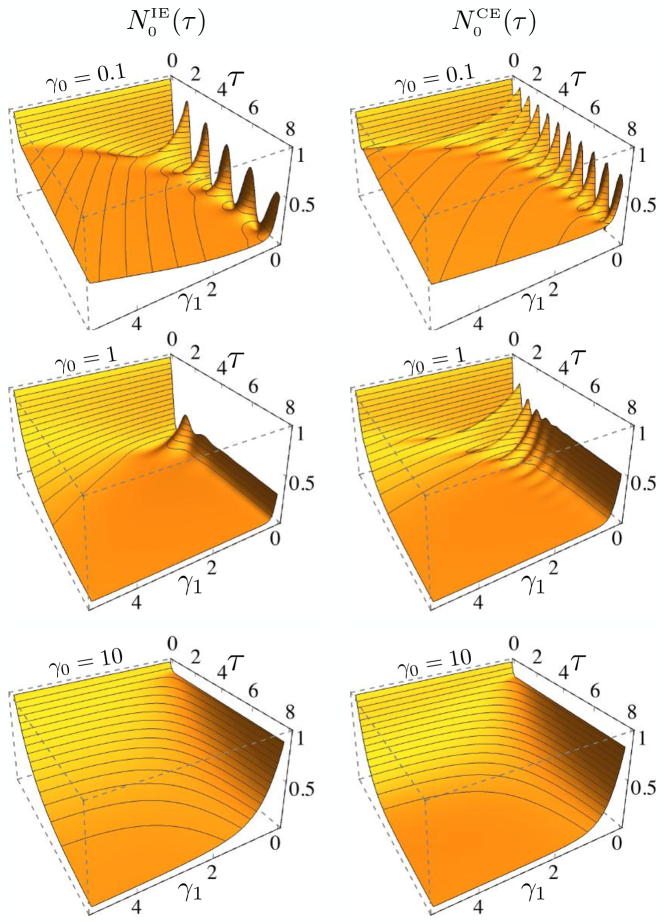
Figure 1: Dynamics of entanglement of the two qubits subject to independent (left column) and a common (right column) URT as a function of the dimensionless time $\tau$ and the switching rate $\gamma_{\hbox{\tiny{1}}}$, for different values of the switching rate $\gamma_{\hbox{\tiny{0}}}$. From top to bottom we have $\gamma_{\hbox{\tiny{0}}}=0.1,1,10$ in both columns.

In Fig. 1 we show the time evolution of the negativity as a function of the dimensionless time $\tau$ for different values of the switching rates $\gamma_{\hbox{\tiny{0}}}$ and $\gamma_{\hbox{\tiny{1}}}$ for both independent and common URT. A large variety of behaviors emerge: there exists values of the switching rates for which the negativity evolves monotonically in time, while for others it display oscillations. In addition, there are regimes in which it decays to zero and other in which it saturates to a certain value. Typically, for small values of the switching rates revivals of quantum correlations are present. On the contrary, very large values of $\gamma_{\hbox{\tiny{0}}}$ and $\gamma_{\hbox{\tiny{1}}}$ lead to a monotonic evolution in time. In the intermediate regime, where one switching rate is large and the other small, revivals are present if the switching rates belong the a specific region of the parameter space $\{\gamma_{\hbox{\tiny{0}}},\gamma_{\hbox{\tiny{1}}}\}$, as shown in Fig. 2. When revivals are present, the effect of a common environment is to double the frequency of the oscillations and to increase their height compared to independent URT, thus leading to stronger quantum correlations. On the contrary, in case of a monotonic behavior, the effect of a common environment is to lead to a faster loss of correlations. The cusps in Fig. 2 correspond to $\gamma_{\hbox{\tiny{0}}}=\gamma_{\hbox{\tiny{1}}}=2$ for independent environments, and to $\gamma_{\hbox{\tiny{0}}}=\gamma_{\hbox{\tiny{1}}}=4$ for common environments.
In order to complete our analysis, we also consider a third scenario, where only one qubit is subject to URT, e.g. $B_{1}(t)=0$ in eq.(2). We suppose the the qubit pair is initially in a Bell state. The dynamics of negativity for all four Bell states then reads:

$$N^{\text{\tiny 1q}}(\tau)=\frac{1}{2}\left(|\Lambda^{u}_{-2}|+|\Lambda^{u}_{2}|\right)=|\Lambda^{u}_{2}|.$$ (20)

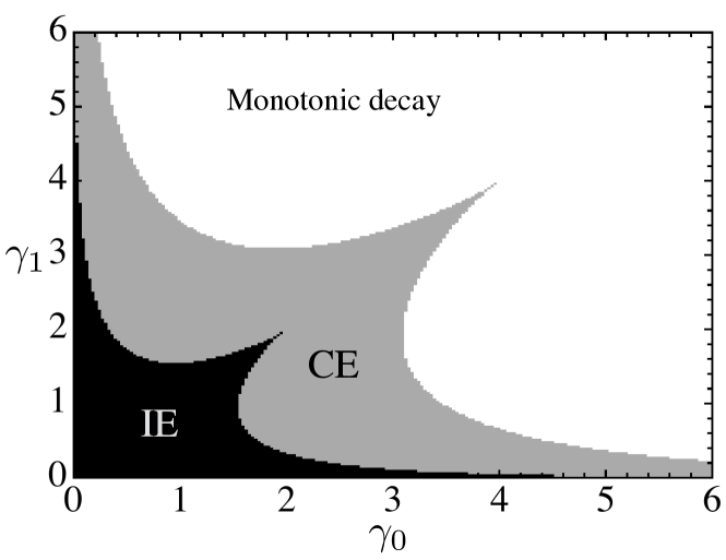
Figure 2: Revivals of entanglement. The shaded areas represent the regions of the parameter space $\{\gamma_{\hbox{\tiny{0}}},\gamma_{\hbox{\tiny{1}}}\}$ in which one observes oscillation in the entanglement dynamics. The black area is for independent environmentsm and the gray one for common environments. The cusps correspond to $\gamma_{\hbox{\tiny{0}}}=\gamma_{\hbox{\tiny{1}}}=2$ for independent environments, and to $\gamma_{\hbox{\tiny{0}}}=\gamma_{\hbox{\tiny{1}}}=4$ for common environments.

4 Non-Markovianity of URT dephasing

As mentioned in Section A.1, the optimal trace distance of the dephasing map is given by the absolute value of the decoherence factor, see Eq. (15). Moreover, we numerically investigate the optimal pair in the case of two qubits subject to local independent environments, and we found that the initial states $|\!+\!+\rangle\!\rangle$ and $|\!-\!-\rangle\!\rangle$ yield the maximum trace distance. A trivial calculation shows that the corresponding trace distance is equal to the absolute value of the decoherence factor (15). This means that the single-qubit and two-qubit non-Markovianity coincides and the optimal trace distance reads:

$$D(\tau) =|\Lambda_{-2}^{a}(\gamma_{\hbox{\tiny{0}}},\gamma_{\hbox{\tiny{1}}},\tau)|=|\Lambda_{2}^{a}(\gamma_{\hbox{\tiny{0}}},\gamma_{\hbox{\tiny{1}}},\tau)|,$$ (21)

with the corresponding information flow:

$$\dot{D}[\tau]=\Lambda^{a}_{2}(\gamma_{\hbox{\tiny{0}}},\gamma_{\hbox{\tiny{1}}},\tau)\,\frac{d}{dt}\Lambda^{a}_{-2}(\gamma_{\hbox{\tiny{0}}},\gamma_{\hbox{\tiny{1}}},\tau)+c.c.$$ (22)

where $c.c.$ stands for complex congiugate. Inserting this expression into Eq. (38), we obtain the expression for BLP non-Markovianity. We report the behavior of $\mathcal{N}(\tau)$ at time $\tau=10$ in Fig. 3 as a function of $\gamma_{\hbox{\tiny{0}}}$ and $\gamma_{\hbox{\tiny{1}}}$. In order to understand the behavior of the non-Markovianity, we first recall that BLP measure of non-Markovianity is different from zero only if there are revivals in the optimal trace distance. The expression of the optimal trace distance in Eq.(15) exactly coincides with the entanglement, quantified by the concurrence, between a single qubit and an ancilla system liu11 . Moreover, we notice that we have already analyzed a similar expression in studying entanglement between two interacting qubits, see Eq.(17). This means that the regions of the parameter space for which entanglement has revivals coincides exactly with the region where the optimal trace distance has revivals, i.e. BLP measure is non-zero. We may now easily illustrate the the behavior shown in the main panel of Fig. 3: the BLP measure is different from zero for the values $\{\gamma_{\hbox{\tiny{0}}},\gamma_{\hbox{\tiny{1}}}\}$ that lies inside the black area in Fig. 2. This may be seen also in the inset, which shows slices of the 3D plot for fixed values of $\gamma_{\hbox{\tiny{0}}}$, i.e. the behavior of non-Markovianity as a function of $\gamma_{\hbox{\tiny{1}}}$ for different fixed values of $\gamma_{\hbox{\tiny{0}}}$.

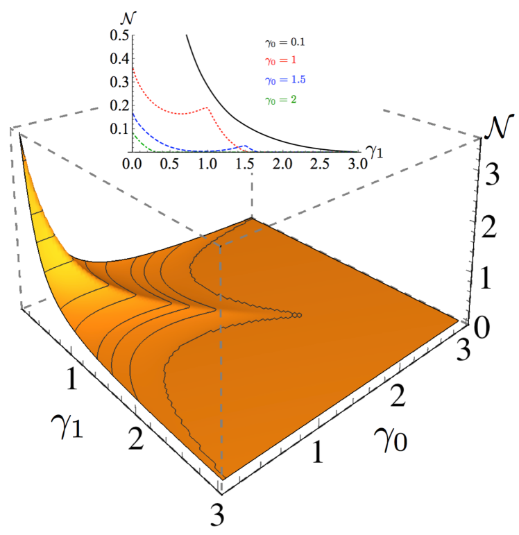
Figure 3: Main panel: BLP measure of Non-Markovianity as a function of $\gamma_{\hbox{\tiny{0}}}$ and $\gamma_{\hbox{\tiny{1}}}$ calculated at time $\tau=10$. The inset shows slices of the 3D plot for fixed values of $\gamma_{\hbox{\tiny{0}}}$, i.e. the behavior of non-Markovianity as a function of $\gamma_{\hbox{\tiny{1}}}$ for different fixed values of $\gamma_{\hbox{\tiny{0}}}$.

For BRT noise benedetti14 , there is a threshold at $\gamma=2$, separating Markovian and non-Markovian dynamics. In the present case of URT a more complex structure arises, and the threshold for backflow of information changes according to fig. 3. We notice also that the balanced case coincides with the cusp at $\gamma_{\hbox{\tiny{0}}}=\gamma_{\hbox{\tiny{1}}}$ and, in general, do not coincide with the largests values of non-Markovianity, i.e. imbalance leads to stronger memory effects. From the inset of Fig. 3 we also see that a general feature of NM is that the smaller the values of the switching rates, the larger the value of NM. Already when one of the switching rate starts to increase, NM quickly vanishes, confirming the idea that slow noise is connected to non-Markovian dynamics.

5 Noisy quantum teleportation

Here we analyze teleportation fidelity when the Bob’s qubit (qubit 3 in Fig. 5) is subject to URT. This scenario corresponds to the situation where Alice generates the entangled pair and then she sends one qubit to Bob through a channel that is affected by noise. The the initial Bell state $|\frac{\sigma_{0}}{\sqrt{2}}\rangle\!\rangle$ is subject to the decoherent evolution given by

$$R=(\mathbb{I}\otimes\mathcal{E})\left[\left|\left.\!\frac{\sigma_{0}}{\sqrt{2}}\!\right\rangle\!\!\!\right\rangle\!\left\langle\!\!\!\left\langle\!\frac{\sigma_{0}}{\sqrt{2}}\right|\right.\right],$$ (23)

where $\mathcal{E}$ is the quantum map describing the URT dephasing, which induces the dynamical evolution of entanglement given by Eq.(20). The map (23) can be expressed in terms of Kraus operators as:

$$\mathcal{E}[\rho_{0}]=\sum_{k=1}^{2}M_{k}(\tau)\rho_{0}M_{k}^{\dagger}(\tau)$$ (24)

with

$$M_{1}(\tau) =\sqrt{\frac{1-|\Lambda(\tau)|}{2}}\left(\begin{array}[]{ll}-\frac{\Lambda(\tau)}{|\Lambda(\tau)|}&0\\ 0&1\end{array}\right)$$ (27)

$$M_{2}(\tau) =\sqrt{\frac{1+|\Lambda(\tau)|}{2}}\left(\begin{array}[]{ll}\frac{\Lambda(\tau)}{|\Lambda(\tau)|}&0\\ 0&1\end{array}\right)$$ (30)

and $\Lambda(\tau)=\Lambda^{a}_{2}(\tau,\gamma_{\hbox{\tiny{0}}},\gamma_{\hbox{\tiny{1}}})$ is the URT dephasing factor of Eq. (12). In the case of balanced RTN, Eq. (24) reduces to the more familiar expression:

$$\mathcal{E}^{s}[\rho_{0}]=\frac{1-\Lambda(\tau)}{2}\,\sigma_{3}\,\rho_{0}\sigma_{3}+\frac{1+\Lambda(\tau)}{2}\rho_{0},$$ (31)

with $\Lambda(\tau)=\Lambda^{s}_{2}(\tau,\gamma)$ the dephasing factor in Eq. (10). By explicitly calculating the evolution in (23), we obtain:

$$R(\tau)=\frac{1}{2}\Big{(}\left|\left.\!M_{1}(\tau)\,\!\right\rangle\!\!\!\right\rangle\left\langle\!\!\!\left\langle\!\,M_{1}(\tau)\right|\right.+\left|\left.\!M_{2}(\tau)\,\!\right\rangle\!\!\!\right\rangle\left\langle\!\!\!\left\langle\!\,M_{2}(\tau)\right|\right.\Big{)}$$ (32)

where we used the property $O_{1}\otimes O_{2}|\psi\rangle\!\rangle=|O_{1}\psi\,O_{2}^{T}\rangle\!\rangle$. After straightforward calculations paris12 , we obtain Bob’s conditional state

$$\rho_{\psi}(\tau)=\sum_{j=1}^{2}\sigma_{k}\,M_{j}(\tau)\,\sigma_{k}\,P_{\psi}\,\sigma_{k}\,M_{j}^{*}(\tau)\sigma_{k}\,.$$ (33)

When $\Lambda(\tau)=1$, we recover the noiseless case which allows one to perfectly teleport the initial state. In the most general case, the input-output fidelity is given by

$$F(\tau)=\frac{1}{2}\Big{\{}1+\mathcal{R}[\Lambda(\tau)]+\big{(}1-\mathcal{R}[\Lambda(\tau)]\cos^{2}\theta\big{)}\Big{\}}$$ (34)

where $\mathcal{R}[x]$ stands for the real part of $x$. The corresponding average fidelity, see Eq. (16), reads as follows

$$F_{av}(\tau)=\frac{1}{3}\Big{(}2+\mathcal{R}[\Lambda(\tau)]\Big{)}\,.$$ (35)

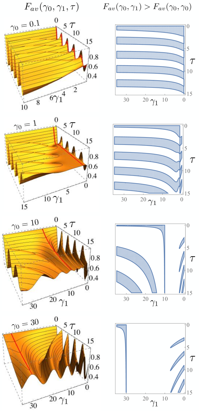
Figure 4: Left column: Average fidelity as a function of the dimensionless time $\tau$ and the switching rate $\gamma_{\hbox{\tiny{1}}}$, for different values of $\gamma_{\hbox{\tiny{0}}}=0.1,\,1,\,10,\,30$ from top to bottom. The red lines are guides for the eye highlighting the case $F_{av}(\gamma_{\hbox{\tiny{0}}},\gamma_{\hbox{\tiny{0}}},\tau)$. Right column: Area in the $\{\gamma_{\hbox{\tiny{1}}},\tau\}$ parameter-space where $F_{av}(\gamma_{\hbox{\tiny{0}}},\gamma_{\hbox{\tiny{1}}},\tau)>F_{av}(\gamma_{\hbox{\tiny{0}}},\gamma_{\hbox{\tiny{0}}},\tau)$, for the same values of $\gamma_{\hbox{\tiny{0}}}$ represented in the left column ($\gamma_{\hbox{\tiny{0}}}=0.1,\,1,\,10,\,30$ from top to bottom).

The behavior of the average fidelity is shown in Fig. 4. On the left column we show $F_{av}$ as a function of the dimensionless time and the switching rate $\gamma_{\hbox{\tiny{1}}}$, for different values of $\gamma_{\hbox{\tiny{0}}}$. Different temporal behaviors arise, depending on the values the switching rates. Indeed, as a function of time, it is possible to find either non-monotonic $F_{av}$ or monotonic decaying average fidelity. Although it is not trivial to describe the different regimes for the fidelity in general, some features emerge. Oscillations are present either when the two values of the switching rates are small or when one is small and the other large. In the last case, oscillations usually achieve a larger amplitude. This has a clear physical interpretation: if one can tune the length of the Bob’s noisy channel such that it corresponds to a maximum in the fidelity oscillation, it is possible to teleport the inital state with fidelity almost equal to one. Another feature emerging from the plot is that $F_{av}(\gamma_{\hbox{\tiny{0}}},\gamma_{\hbox{\tiny{0}}},\tau)$ has a monotonic behavior for any $\gamma_{\hbox{\tiny{0}}}>2$. However, even a small unbalance between the two switching rates may again produce revivals in the fidelity $F_{av}(\gamma_{\hbox{\tiny{0}}},\gamma_{\hbox{\tiny{1}}},\tau)$ with $\gamma_{\hbox{\tiny{0}}},\gamma_{\hbox{\tiny{1}}}>2$.

In the right column of Fig. 4, we compare the value of the average fidelity in the case of URT with the case of BRT. We notice that there exist values of the parameters for which the fidelity in the case of URT is larger than that obtained in the presence of BRT, meaning that the quantum teleportation performances can be improved by unbalancing the switching rates. Moreover, as it is apparent from the plots, when the switching rates are small, it is very easy to outperform fidelity of the balanced case (see for example the first plot on the right column). On the contrary, the region of the parameter space that allows one to exceed the BRT fidelity for large rates is very small (see bottom plot on the right column) and it becomes difficult to improve the performances of the teleportation protocol in the case of BRT with large switching rates. Analogous considerations can be made if we modify the teleportation protocol to add noise on both parties, i.e. both Alices’s and Bob’s qubit are subject to local and independent URT. In this case, the Hamiltonian is described by Eqs. (1) and (2) with $B_{1}(t)\neq B_{2}(t)$ and a simple calculation leads to an average fidelity:

$$F_{av}(\tau)=\frac{1}{3}\left(2+\mathcal{R}\left[\Lambda^{2}(\tau)\right]\right).$$ (36)

Teleportation is based upon the presence of entanglement, however the expression of the average fidelity is not directly related to the negativity , since the first depends on the real part of $\Lambda(\tau)$ or $\Lambda^{2}(\tau)$ (cfr Eqs. (35) and (36)), while entanglement varies as their absolute value (see Eqs. (20) and (17)). In the case of balanced RTN revivals in the fidelity and entanglement coincides , since $\Lambda(\tau)$ is a real quantity, but in the most general case of URT this is not true, and there is not a simple connection between the temporal behaviors of the two quantities.

6 Conclusions

We have addressed the dynamics of quantum correlations in a two-qubit system subject to unbalanced random telegraph noise and have discussed in details the similarities and the differences with the balanced case. In particular, we have analyzed the effect of URT noise on entanglement, non-Markovianity and teleportation fidelity, and have individuated different working regimes.

We have found that entanglement of an initial Bell pair subject to either independent or common environments shows revivals as a function of time in a specific region of the $\{\gamma_{\hbox{\tiny{0}}},\gamma_{\hbox{\tiny{1}}}\}$ parameter space. A common environment leads to faster oscillations and to a stronger non-monotonic behavior, i.e a larger region in the parameter space leading to oscillations. We have linked revivals of entanglement (with independent environments) to non-Markovianity of the two-qubit map. This is due to the fact that both quantities depend on the absolute values of the decoherence factor. Finally, we have addressed fidelity of teleportation protocol for the shared Bell state subject to (one-side) URT dephasing and found that fidelity depends on the real part of the decoherence factor. A variety of different behaviors arose, ranging from a monotonic-decaying to the presence of revivals, with unbalanced noise that allows one to increase fidelity with respect to the balanced case.

Overall, our results show that noise imbalance may be exploited to mitigate decoherence and preserve teleportation fidelity, thus suggesting that even a modest engineering of environment, in the direction of making the switching rates different, permits to better preserve quantum features and, in turn, to improve performances of quantum information protocols in the presence of noise.

Author contribution statement

SD, CB and MGAP contributed to the design and implementation of the research, to the analysis of the results and to the writing of the manuscript.

Appendix A Appendix

In this appendix we review the definitions of the non-Markovianity in terms of information backflow and we review the teleportation protocol.

A.1 Quantification of (quantum) non-Markovianity

In classical physics, a Markovian process usually refers to a stochastic model where the probability distribution of the events depends only on the state attained in the previous event. Non-Markovianity (NM) is accordingly defined as the violation of this conditions, and usually involves the appearance of memory effects in the dynamics of the considered systems. When one moves to open quantum systems, one realises that memory effects play an important role and, together with entanglement, represents a resource for quantum information technology. Indeed, memory effects may mitigate the detrimental effects of the interaction with the external environment, such that quantum coherence may be preserved longer. This prompted efforts to precisely define the notion of NM for quantum processes, a task which have been pursued in different ways, with reference to different mathematical properties of the quantum dynamical map.

In this paper, we stick with the BLP measure of non-Markovianity blp , where Markovianity is thus seen as an irreversible flow of information from the system to the environment, while non-Markovianity allows for the information to flow back into the system. Distinguishability between any two states can be defined using the trace distance :

$$D[\rho_{1},\rho_{2}]=\frac{1}{2}\|\rho_{1}-\rho_{2}\|_{1}.$$ (37)

which provides a metric in the Hilbert space of physical states. The trace distance takes values between 0 and 1 for indistinguishable and orthogonal states respectively. Moreover, it is invariant under unitary transformations $U$, $UU^{\dagger}=U^{\dagger}U={\mathbb{I}}$, i.e. $D[U\rho_{1}U^{\dagger},U\rho_{2}U^{\dagger}]=D[\rho_{1},\rho_{2}]$, and it is contractive, i.e. $D[\Phi\rho_{1},\Phi\rho_{2}]\leq D[\rho_{1},\rho_{2}]$, for any completely positive and trace-preserving map $\Phi$. If the distinguishability between states decreases, information flows out of the system into the environment, and the two expression above just express the facts that information is preserved in closed systems, and that the maximum amount of information that can be recovered by the system cannot be larger than the amount that flowed out of it.

In order to measure the degree of NM, one has to introduce the information flow $\dot{D}=\frac{d}{d\tau}D[\rho_{1}(\tau),\rho_{2}(\tau)]$ where $\rho_{12}(0)$ represent a pair of initial states. A $\dot{D}>0$ means a reversed flow of information. For non-Markovian processes, there exist at least one pair of initial states and a temporal interval in which $\dot{D}$ is positive, meaning that the trace distance between the initial states is increasing, i.e. information is flowing back. The BLP measure of non-Markovianity quantifies the growth in distinguishability, related to the total amount of information backflow, i.e.

$$\mathcal{N}\!(\tau)=\underset{\rho_{12}(0)}{\max}\,\underset{\dot{D}>0}{\int_{0}^{\tau}}\dot{D}[s,\rho_{12}(0)]ds.$$ (38)

where the maximum is evaluated taking into account all pairs of initial states. The dynamics of the system is thus non-Markovian when $\mathcal{N}>0$.

A.2 Teleportation

Quantum teleportation is a protocol where entanglement is exploited in order to transmit an unknown quantum state $|\psi\rangle=\cos\frac{\theta}{2}|0\rangle+e^{i\phi}\sin\frac{\theta}{2}|1\rangle$ from Alice (A) to Bob (B) without physically sending the qubit. In order for teleportation to work exactly, A and B need to share a maximally entangled state, e.g. $|\frac{\sigma_{0}}{\sqrt{2}}\rangle\!\rangle$. The overall input state is the three-qubit state $|\psi\rangle_{\text{\scriptsize\!1}}\otimes|\frac{\sigma_{0}}{\sqrt{2}}\rangle\!\rangle_{\text{\scriptsize\!23}}$. Then Alice performs a Bell measurement $\Pi_{k}=|\frac{\sigma_{k}}{\sqrt{2}}\rangle\!\rangle_{\text{\scriptsize\!12}}\,{}_{\text{\scriptsize\!12}}\langle\!\langle\frac{\sigma_{k}}{\sqrt{2}}|$ on her qubits (see the protocol scheme in Fig. 5).

Figure 5: Quantum teleportation protocol. A and B share a maximally entangled state, then Alice performs a Bell measurement on qubits $1\&2$ and communicates which results she got to Bob, who performs a suitable unitary transformation on his conditional state. The protocol works with neither Alice, nor Bob, knowing which state $|\psi\rangle$ is being teleported.

The state of qubit $3$, conditional to Alice obtaining the result $k$, is given by $\eta_{\psi,k}=\sigma_{k}\,P_{\psi}\,\sigma_{k}$ where $P_{\psi}=|\psi\rangle\langle\ \psi|$ is the projector of over the initial state of qubit $1$. In order to retrieve the input state, Bob should know which operation to perform in order to correct the effects of the reduction postulate. To this purpose, Alice communicates to Bob though a classical channel which results she has got. Bob then implements a suitable unitary $V_{k}=\sigma_{k}$ on his qubit, obtaining the output state of the protocol $\rho_{\psi}=\sigma_{k}\eta_{\psi,k}\sigma_{k}=P_{\psi}$, $\forall k$, which is the input state that we wanted to teleport. We remind that the protocol works with neither Alice, nor Bob, knowing the teleported state.

References

- (1) D. Loss, D. P. DiVincenzo, Quantum computation with quantum dots, Phys. Rev. A 57, 120 (1998).
- (2) B. E. Kane, Silicon-based quantum computation, Progr. Phys. 48, 1023 (2000).
- (3) D. J. Reilly, Engineering the quantum-classical interface of solid-state qubits, NPJ Quantum Inf. 1, 15011 (2015)/
- (4) M. Weissman, et al., 1/f noise and other slow, nonexponential kinetics in condensed matter, Rev. Mod. Phys. 60, 537 (1988).
- (5) E. Paladino, et al., 1/f noise: Implications for solid-state quantum information, Rev. Mod. Phys. 86, 361 (2014).
- (6) Y. Makhlin, G. Schön, and A. Shnirman, Quantum-state engineering with Josephson-junction devices, Rev. Mod. Phys. 73, 357 (2001).
- (7) Y. Nakamura, C. D. Chen, and J. S. Tsai, Spectroscopy of energy-level splitting between two macroscopic quantum states of charge coherently superposed by Josephson coupling, Phys. Rev. Lett. 79, 2328 (1997).
- (8) Y. Nakamura, Yu. A. Pashkin, and J. S. Tsai, Coherent control of macroscopic quantum states in a single-Cooper-pair box, Nature 398, 786 (1999).
- (9) J. E. Mooij, et al., Josephson Persistent-Current Qubit, Science 285, 1036 (1999).
- (10) J. R. Friedman, et al., Quantum superposition of distinct macroscopic states, Nature 406, 43 (2000).
- (11) T Fujisawa, et al., Spontaneous Emission Spectrum in Double Quantum Dot Devices, Science 282, 932 (1998).
- (12) J. R. Petta et al., Coherent Manipulation of Coupled Electron Spins in Semiconductor Quantum Dots, Science 309, 2180 (2005).
- (13) Z. Shi, et al., Fast Hybrid Silicon Double-Quantum-Dot Qubit, Phys. Rev. Lett. 108, 140503 (2012).
- (14) T. Itakura and Y. Tokura, Dephasing due to background charge fluctuations, Phys. Rev. B 67, 195320 (2003).
- (15) X. Hu and S. Das Sarma, Charge-Fluctuation-Induced Dephasing of Exchange-Coupled Spin Qubits, Phys. Rev. Lett. 96, 100501 (2006).
- (16) J. K. Gamble,et al., Two-electron dephasing in single Si and GaAs quantum dots, Phys. Rev. B 86, 035302 (2012).
- (17) A. B. Zorin, et. al., Background charge noise in metallic single-electron tunneling devices, Phys. Rev. B 53, 13682 (1996).
- (18) V. A. Krupenin, et al., Noise in al single electron transistors of stacked design, J. Appl. Phys. 84, 3212 (1998).
- (19) S. W. Jung, et. al, Background charge fluctuation in a GaAs quantum dot device, Appl. Phys. Lett. 85, 768 (2004).
- (20) R. L. Stoop, et al., Charge Noise in Organic Electrochemical Transistors, Phys. Rev. Applied 7, 014009 (2017).
- (21) C. Kurdak, et al., Resistance fluctuations in GaAs/As quantum point contact and Hall bar structures, Phys Rev. B 56, 9813 (1997).
- (22) K. S. Ralls, et al., Discrete Resistance Switching in Submicrometer Silicon Inversion Layers, Phys. Rev. Lett. 52, 228 (1984).
- (23) M. J. Kirton and M. J. Uren, Noise in solid-state microstructures: A new perspective on individual defects, interface states and low-frequency ()noise, Adv. in Phys., 38, 367 (1989).
- (24) J. Sung-Min , et al., Threshold Voltage Fluctuation by Random Telegraph Noise in Floating Gate NAND Flash Memory String, IEEE Trans. Electron Devices, 58, 67 (2011).
- (25) B. Kaczer, et al., Gate current random telegraph noise and single defect conduction, Microelectron. Eng. 109 123 (2013) .
- (26) R. Black, et al.,Nearly traceless 1/f noise in bismuth, Phys. Rev. Lett. 51, 1476 (1983).
- (27) A. Ludviksson, et al.,Low-frequency 1/f fluctuations of resistivity in disordered metals, Phys. Rev. Lett. 52, 950 (1984).
- (28) D. J Reilly, Engineering the quantum-classical interface of solid-state qubits, Quantum Inf. 1, 15011 (2015).
- (29) L. DiCarlo et al., Demonstration of two-qubit algorithms with a superconducting quantum processor, Nature 460, 240 (2009).
- (30) L. Steffen et. al, Deterministic quantum teleportation with feed-forward in a solid state system, Nature 500, 319 (2013).
- (31) M. Hirose and P. Cappellaro, Coherent Feedback Control of a Single Qubit in Diamond, Nature 532, 77 (2016).
- (32) C. Benedetti, F. Buscemi, P. Bordone, and M. G. A. Paris, Effects of classical environmental noise on entaglement and quantum discord dynamics, Int. J. Quantum Inf. 10, 1241005 (2012).
- (33) C. Benedetti, M. G. A. Paris, and S. Maniscalco, Non-Markovianity of colored noisy channels, Phys. Rev. A 89, 012114 (2014).
- (34) W. K. Wootters, Philosophical Transactions: Mathematical, Physical and Engineering Sciences 356, 1717 (1998).
- (35) B. Bylicka, D. Chruściński and S. Maniscalco Non-Markovianity and reservoir memory of quantum channels: a quantum information theory perspective, Sci. Rep. 4, 5720 (2014).
- (36) D. R. Cox and H. D. Miller, The Theory of Stochastic Processes, (Wiley, New York, 1965), p. 172.
- (37) R. Fitzhugh, Math. Biosc. 64, 75 (1983).
- (38) T. M. Buehler, et al., Observing sub-microsecond telegraph noise with the radio frequency single electron transistor, J. Appl. Phys. bf 96, 6827 (2004).
- (39) T. Fujisawa and Y. Hirayama, Charge noise analysis of an AlGaAs/GaAs quantum dot using transmission-type radio-frequency single-electron transistor technique, Appl. Phys. Lett. 77, 543 (2000).
- (40) J. Kamioka, et al., Charge noise analysis of metal oxide semiconductor dual-gate Si/SiGe quantum point contacts, New J. Phys. 11, 025002 (2009).
- (41) J. Bergli, Y. M. Galperin, and B. L. Altshuler, Decoherence of a qubit by non-Gaussian noise at an arbitrary working point, Phys. Rev. B 74, 024509 (2006).
- (42) J. Bergli, Y. M. Galperin, and B. L. Altshuler, Decoherence in qubits due to low-frequency noise, New J. Phys. 11, (2009).
- (43) J. Fern, Expectations of two-level telegraph noise, arXiv:quant-ph/0611020.
- (44) R. Horodecki, P. Horodecki, M. Horodecki, and K. Horodecki, Quantum entanglement, Rev. Mod. Phys. 81, 865 (2009)
- (45) O. Gühne and G. Tóth, Entanglement detection, Phys. Rep. 474 1-79 (2009).
- (46) M. B. Plenio, and S. Virmani, An introduction to entanglement measures, Quant. Inf. Comput. 7, 1 (2007).
- (47) G. Vidal and R. F. Werner, Computable measure of entanglement, Phys. Rev. A 65, 032314 (2002)
- (48) B.-H. Liu, et al., Experimental control of the transition from Markovian to non-Markovian dynamics of open quantum systems, Nat. Phys. 7, 931 (2011).
- (49) M. G. A. Paris, The modern tools of quantum mechanics. A tutorial on quantum states, measurements, and operations , Eur. Phys. J. Special Topics 203 61 (2012).
- (50) E.-M. Laine, H.-P. Breuer and J. Piilo, Nonlocal memory effects allow perfect teleportation with mixed states, Sci. Rep. 4, 4620 (2014).
- (51) Y. Dong, Y. Zheng, S. Li, C.-C. Li, X.-D. Chen, G.-C. Guo and F.-W. Sun, Non-Markovianity-assisted high-fidelity Deutsch-Jozsa algorithm in diamond, Quantum Inf. 4, 3 (2018).
- (52) H.-P. Breuer, E. M. Laine, and J. Piilo, Measure for the Degree of Non-Markovian Behavior of Quantum Processes in Open Systems, Phys. Rev. Lett. 103, 210401 (2009).
- (53) Z. He, J. Zou, L. Li, and B. Shao, Effective method of calculating the non-Markovianity for single-channel open systems, Phys. Rev. A 83, 012108 (2011).