Seeing the Wood for the Trees: Reliable Localization
in Urban and Natural Environments

Abstract

In this work we introduce Natural Segmentation and Matching (NSM), an algorithm for reliable localization, using laser, in both urban and natural environments. Current state-of-the-art global approaches do not generalize well to structure-poor vegetated areas such as forests or orchards. In these environments clutter and perceptual aliasing prevents repeatable extraction of distinctive landmarks between different test runs. In natural forests, tree trunks are not distinctive, foliage intertwines and there is a complete lack of planar structure. In this paper we propose a method for place recognition which uses a more involved feature extraction process which is better suited to this type of environment. First, a feature extraction module segments stable and reliable object-sized segments from a point cloud despite the presence of heavy clutter or tree foliage. Second, repeatable oriented key poses are extracted and matched with a reliable shape descriptor using a Random Forest to estimate the current sensor’s position within the target map. We present qualitative and quantitative evaluation on three datasets from different environments - the KITTI benchmark, a parkland scene and a foliage-heavy forest. The experiments show how our approach can achieve place recognition in woodlands while also outperforming current state-of-the-art approaches in urban scenarios without specific tuning.

I Introduction

Localization is an important problem in autonomous robot navigation when surveying challenging environments such as forests, oil rigs, and disaster response sites or teach-and-repeat operations in orchards for disease detection and analysis of tree growth. Systems should be able to recognize places in both urban and vegetated areas, while being resilient to appearance changes caused by the robot’s motion, occluding clutter or temporal variations of the environment.

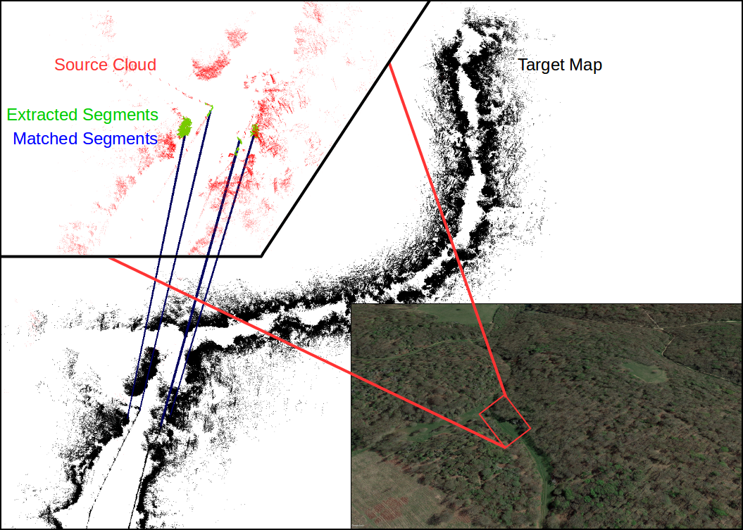
Figure 1: The proposed approach provides reliable segmentation (green) and matching (blue lines) of objects such as trees and bushes within natural, forested environments. The current source point cloud (red) is shown in the top left corner. The blue lines indicate the localization estimate relative to the target map (black), consisting of a previously traversed $\sim 1\text{km}$ route within a forest.

There has been extensive study of localization in indoor or outdoor structured environments using vision or laser sensors. Strategies are often split into two parts - global registration approaches which match high level features within a large map [1, 2, 3], and fine registration methods that perform point-wise refinements [4, 5]. These strategies often rely on landmark correspondences between candidate point clouds, implicitly assume built environments, containing planar objects, or require reliable normal estimation and consistent data association.

The problem of place recognition in structure-poor scenarios is less well explored. Current approaches model natural environments specifically, using state machines to aid their place recognition systems based on prior knowledge about the dataset [6, 7]. It is common to specifically model the canopy of trees or bushes. The foliage in vegetated areas changes with vegetation growth or pruning, and is also affected by continuous seasonal alteration. In addition, defining an accurate localization is difficult because the tree canopy can be interleaved and heavy foliage/clutter can obscure stable landmarks.

It is currently unclear how localization approaches will transfer to the more challenging environments we are interested in. Designing algorithms to be invariant to the type of environment and geometrical differences may result in performance improvement. In this work we bridge the gap between structured urban environments and challenging natural environments without explicitly modelling every orchard or forest individually by using more repeatable and descriptive features.

The main contribution of our work is a method that enables global place recognition in three different scenery settings. Our approach adapts the framework from [2] to reliably extract segments from natural environments which carry repeatable and distinctive information from a source point cloud and utilize them to solve global registration to a target map (Fig. 1). The pipeline of our approach is illustrated in Fig. 2.

Our contributions are as follows:

1. we propose an extension of the SegMatch approach [2] for place recognition in both urban and natural environments, which we call Natural Segmentation and Matching (NSM),

2. we identify and evaluate a novel combination of key pose extraction and description methods. The key pose extraction module segments and defines consistent orientated coordinate frames for object-sized segments despite the presence of heavy clutter. The descriptor carries sufficient information to recognize different instances of the same segment, achieving a higher accuracy with respect to previous approaches,

3. we perform a thorough evaluation of the approach across datasets captured in an urban area, a parkland scene and a foliage-heavy forest.

The remaining sections of the paper are structured as follows: Sec. II presents the literature review, Sec. III outlines each module of our algorithm, and Sec. IV extensively evaluates the approach. We discuss interesting findings and limitations of our approach in Sec. V.

II Related Work

Global localization is commonly solved by directly extracting and describing keypoints from a point cloud [1, 8, 9], or by segmenting objects in the scene and matching those to a prior map [2, 3]. A coarse alignment is computed that can later be refined with methods like the Iterative Closest Point (ICP) [10]. The task is more challenging in natural environments, as keypoint extraction or segmentation methods often assume some regular structure in the environment.

Place recognition strategies

Bosse and Zlot [8] presented three different methods for keypoint selection that were described with model grid descriptors. The descriptors’ dimensions were later normalized using a nonlinear normalization function and reduced to increase efficiency and reduce the signal-to-noise ratio. Place recognition was achieved by keypoints voting for their closest neighbour in a previous database of keypoints. Their work was extended in [9] to support 3D regional point descriptors.

Elbaz et al. [3] utilized a Random Sphere Cover Set (RSCS) to divide a point cloud into a set of super-points clusters. Each point can be a part of multiple super-points, resulting in the point cloud being separated by overlapping spheres. These spheres were projected as depth map images and fed into a Deep Auto-Encoder network to generate feature descriptors. Candidate matches are selected using a K-nearest neighbors (k-NN) search. In their approach when segmenting the point clouds into RSCS, the authors assumed that each super-point described a surface.

Dubé et al. [2] presented SegMatch. This approach segmented the target and source point clouds using Euclidean clustering. These clusters were matched using k-NN and predictions from a Random Forest, trained on an Eigenvalue-based and Ensemble of Shape Histogram features. The centroids of the matched segments were then used to produce a 6-DoF pose estimate for the sensing vehicle using RANSAC. The approach assumes that the centroid (mean) of all points is a representative point of a cluster, which unfortunately does not hold in natural environments.

Figure 2: The proposed approach.

Localization in Natural Environments

Some of the challenges in natural environments include occlusions, clutter or branch deformations, unstable normal extraction, predominance of structure-poor objects. These are usually the result of interleaved trees or even just windy conditions. Thus most state-of-the-art approaches performing place recognition in natural environments rely on explicit assumptions about the model of the scene [6, 7].

Wellington et al. [6] presented an approach for tree segmentation in orchards, utilizing a push-broom laser scanner. The ground surface was estimated using a Markov Random Field, which helped estimating the boundaries between each tree, the height and density of trees. A Hidden Semi-Markov Model modeled the environment using three states - tree, gap or boundary. The approach incorporated a hidden state to account for the explicit prior on tree spacing. Underwood et al. [7] extended this approach to perform tree recognition and platform localization. After segmentation and characterization, the localization problem was modelled as a Hidden Markov Model [11]. The approach was tested in an orchard with regular rows of trees which were clearly delineated.

Bosse and Zlot [1] performed place recognition in natural environments by selecting a set of keypoints from 10% of the densest areas in a point cloud, and computed a local Gestalt descriptor around each of them [8]. The method was evaluated on a natural open eucalyptus forest with multi-use dirt trails, where the densest areas of the point cloud were vegetated. In the proposed work, we utilize a different strategy for keypoint extraction which is based on firstly extracting segments in the environment, which we then append with a common orientation frame and describe using a Gestalt descriptor. A notable difference is that we opted for a learning-based approach when matching between key poses.

In summary, our work differs from the state-of-the-art in place recognition in natural environments in that we utilise segmentation as a prior step for keyframe extraction on natural data. Our work adapts SegMatch [2] to reliably segment key poses in manner which is repeatable between different observations. In addition, we utilise a feature descriptor that describes both the shape of the segment and the corresponding key pose’s neighbourhood, resulting in resilient localization in cluttered natural areas and urban scenarios.

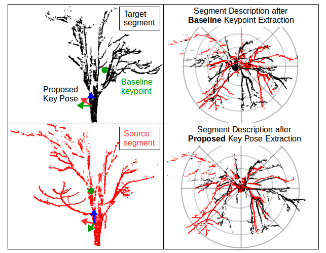
Figure 3: Key pose estimation between two different observations of the same segment: the target map (black) and source cloud (red). The centroid of each segment shown in green, used by a baseline method [2]. The proposed method computes position and orientation for the key pose which is consistent for both the target and source clouds. The figures on the right represent a top view of the segments aligned with either of these two approaches. Subsequently our key pose descriptor can more coherently extract features as the points of each segment occupy the same descriptor bin in the two observations.

III Natural Segmentation and Matching

This section presents the proposed Natural Segmentation and Matching (NSM) approach, which adapts SegMatch [2] for natural environments. We wish to estimate the position of the sensor within a target map using the current source point cloud. The approach focuses on identifying repeatable segments from point clouds captured in cluttered scenes where the detected objects can differ significantly in appearance between observations. We aim to overcome the weaknesses of the previous methods by improving the feature extraction and description steps as follows: A) prior to segmentation, the input clouds are pre-filtered using a Progressive Morphological Filter to discard ground points [12]. Then oriented key poses are computed for each segmented object. This makes the extraction more robust to variation in appearance from different points of view. B) A hybrid feature descriptor is defined using PCA and Gestalt features, which embed sufficient information so as to enable place recognition in both natural and urban environments.

III-A Feature Extraction

Segmentation

We employ Euclidean segmentation, similarly to [2], in order to delineate individual objects such as interleaved trees and bushes. A typical segment corresponds to a tree with a portion of its major branches, a dense bush, a vehicle, some urban structure or any rigid object in the scene with limited physical size. Most clutter is implicitly filtered-out as it does not satisfy criteria about the uniformity of points and dimensions of the segment in question. Care is taken to ensure that it is possible to reliably distinguish a specific object across temporal or spatial variations by assigning a key pose to each segment. Note, that we considered the region-growing approach of [13], however, normals computed in these natural environments are unstable [1].

Oriented Key Pose Extraction

For each segment in the source cloud ${s_{s}}_{i}\in\{{s_{s}}_{1},{s_{s}}_{2}\ldots{s_{s}}_{N}\}$, and in the target map ${s_{t}}_{j}\in\{{s_{t}}_{1},{s_{t}}_{2}\ldots{s_{t}}_{M}\}$, a key pose $\mathbf{k}\in\mathbb{R}^{6}$ needs to be defined. This pose will be used to define the position and orientation of each segment so as to aid the recognition task. An illustration of how a consistent key pose can help mitigate changes in appearance between different points of view is shown in Fig. 3.

We assume that the observed objects are rigidly connected to the ground. This allows us to orient the z-axis of $\mathbf{k}$ as the global up vector, and determine the orientation of the segment based on the predominant dimension along which the points are distributed perpendicularly to z. The x-axis is projected onto the normal direction at $\mathbf{k}$, and the y-axis is computed as the cross product between the x and z axes. Once the orientation is been determined, the key pose’s position $[{k}_{x},{k}_{y},{k}_{z}]$ is calculated as the median of all the points of a subset of $s$ and stored for later use. The median is used instead of the mean so as to mitigate segmentation differences between matching objects as shown on Fig. 3

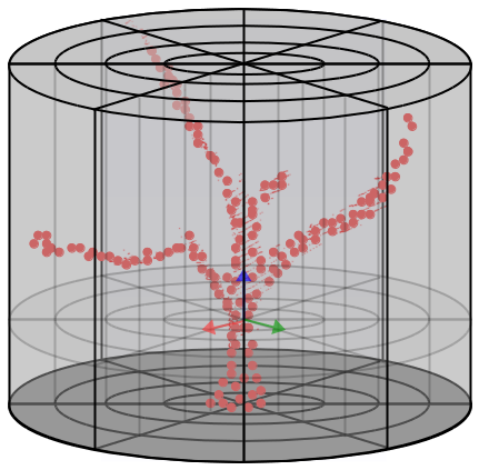
Figure 4: Visual representation of the Gestalt descriptor of a tree segment (red), oriented around the extracted key pose.

III-B Hybrid Feature Description

In the next step, the extracted segments are described in both the target and source clouds using a hybrid feature set combining Eigenvalue features and an adaptation of the Gestalt model [1, 14], illustrated in Fig. 4. Thus, NSM encodes both the geometric properties of the segments and their point distribution.

For each segment $s$, planarity and cylindricality features are computed after PCA. These are, respectively,

$$P_{\lambda}=\lambda_{2}-\lambda_{1}$$ (1)

and

$$C_{\lambda}=\lambda_{3}-\lambda_{2},$$ (2)

where $\lambda_{\{1,2,3\}}$ are to the ordered normalized eigenvalues. The structure tensor is of rank 3 and it follows that $\lambda_{1}\geq\lambda_{2}\geq\lambda_{3}\geq 0$. $P_{\lambda}$ and $C_{\lambda}$ encode the geometric information for each cluster, enabling NSM to account for the rigidity of objects.

Each segment is then split into 4 radial and 8 azimuthal divisions about its key pose’s z-axis and clock-wise starting from the x-axis, resulting in 32 bins. For each bin the mean and variance of the height values of all points are recorded for a total of 64 dimensions. The planarity and cylindricality values are included in the feature vector, resulting in a descriptor of 66 dimensions. In the experimental section we show that such a descriptor carries sufficient information to identify different instances of the same segment in cluttered scenarios.

III-C Feature Matching

Feature matching is performed in two stages using the approach proposed by [2]. Firstly, a k-NN search in feature space creates a list of possible matches for each source segment $s_{s_{i}}$ that matches $K$ target segments using $L_{2}$ distance. Secondly, the list of candidate matches is further refined using a Random Forest (RF) that performs a binary classification over each set of $K$ proposals.

We have trained our RF using the full feature vector dimension while taking into consideration the difference between two matching samples. The input to our RF consists of $(|\mathbf{f}_{s}|,|\mathbf{f}_{t}|,\Delta\mathbf{f})$, where $\mathbf{f}_{s}$ and $\mathbf{f}_{t}$ are the feature vectors corresponding to all source segments and its candidate matches in the target map and $|\cdot|$ denotes the modulus. We consider the descriptor $\Delta\textbf{f}$ to be computed from the difference between each source and target feature vector, that is $\Delta\textbf{f}_{ik}=|\textbf{f}_{s_{i}}-\textbf{f}_{t_{k}}|$ $\forall{i,k}$ with $k\in[1:K]$, which we empirically found to help during the matching task. This is possible as the segments have a consistent orientation after key pose extraction and each feature vector is sorted by definition. The output of the RF classifier is a score $w$, defining the likelihood of a match being correct between segments $s_{s}$ and $s_{t}$. The score is thresholded to produce a set of accepted matches.

	KITTI	George Square Park (GS)	Cornbury Park (CP)
Source	Geiger et al. [16]	Ours	Ours
Environment	Urban, structured	Vegetated, structured,	Vegetated, unstructured,
		well observed trees	hard to delineate trees,
			predominance of bushes
Dynamics	Moving cars, bicycles,	A few moving people	None
	pedestrians
LIDAR	3D HDL-64E @ 10Hz	Push-broom @ 75Hz	3D HDL-32E @ 10Hz
Path	On streets	3 loops on a concrete	Off-road dirt track
		trail in the park	out and back trail
Scene Area	$\sim 500\text{m}$ for localization	$\sim 500\text{m}$ each loop	$\sim 1\text{km}$ each direction
# of Scans	1104	$\sim$ 40700	1823
# of Points	$\sim$ 130000/scan	$\sim$ 381/scan	$\sim$ 70000/scan
Map creation	Scans projected	VO [17] on first loop,	Scans projected on ground
	on ground truth	manual loop closures [18]	truth from forward pass
			locally corrected via ICP
			globally corrected via [18]
Ground Truth	✓	✗	✓
Training Data	KITTI Seq 06	Pre-trained KITTI	Pre-trained KITTI
Testing Data	KITTI Seq 00	Georges Square (GS)	Cornbury Park (CP)
Experiment	Exp. A	Exp. B	Exp. C

TABLE I: Datasets used in our experiments.

III-D Pose Estimation

We utilize the method from [15, 2] in order to maintain geometric consistency between each pair of matches $((\textbf{k}_{s_{p}},\textbf{k}_{t_{p}}),(\textbf{k}_{s_{q}},\textbf{k}_{t_{q}}))\in\mathcal{C}=\{(\textbf{k}_{s_{0}},\textbf{k}_{t_{0}})\ldots(\textbf{k}_{s_{L}},\textbf{k}_{t_{L}})\}$, where $\mathcal{C}$ is the set of accepted matches proposed by the RF and $L$ its cardinality. The formula in Eq. (3) ensures that a pair of matching key poses have similar spatial distances between them.

$$\lvert\lVert\textbf{k}_{t_{p}}-\textbf{k}_{t_{q}}\rVert_{2}-\lVert\textbf{k}_{s_{p}}-\textbf{k}_{s_{q}}\rVert_{2}\rvert<\epsilon$$ (3)

In Eq. (3), $\epsilon$ is the resolution parameter, which determines how similar the source cloud is to the target. The lower the value, the stricter the algorithm behaves. A localization proposal is accepted only if it satisfies a criteria about the minimum number of accepted matches. For a 6-DoF pose to be estimated, there must be at least $\tau=3$ matches. Finally the 6-DoF transform which aligns the source cloud into the target map is computed by a RANSAC optimization on the key poses of the remaining matches.

Parameters
		KITTI	GS	CP
	Min # Points	$200$		$2500$
	Max # Points	$1500$		$50000$
Segmentation	Max Distance	$0.2\text{m}$
Description	Gestalt Radius	$2.0\text{m}$
	K Neighbours	$200$
	# of Trees	$250$
	Tree Depth	$50$
Matching	RF Threshold ($w$)	$0.69$
Pose	Resolution ($\epsilon$)	$0.4\text{m}$
Estimation	Min # Clusters ($\tau$)	$4$

TABLE II: Parameters used in our experiments.

IV Experimental Evaluation

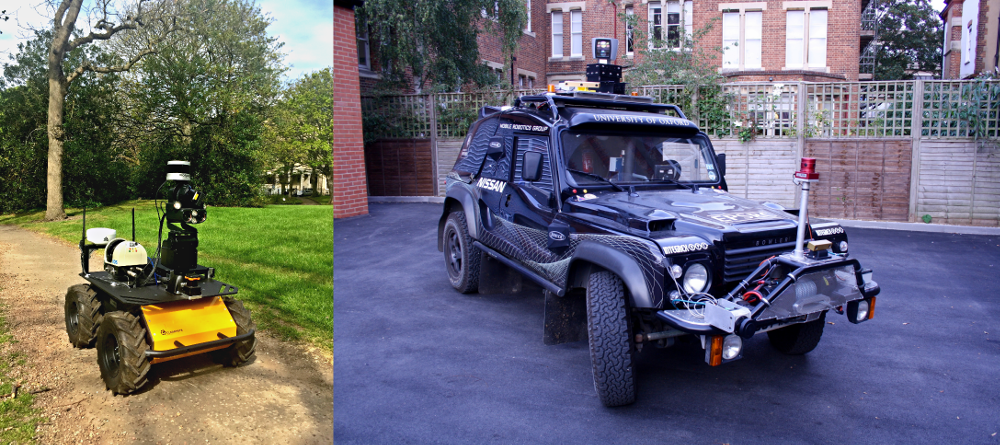
Figure 5: The robots utilised to collect data for our experiments. A Clearpath Husky robot (left) was used to collect the GS dataset with a push-broom LIDAR and a Multisense SL. A Bowler Wildcat platform (right) was utilised to collect the CP dataset, equipped with a Velodyne HDL-32E LIDAR, OxTS GPS, Novatel INS and Bumblebee2 camera.

The main goal of this work is to perform global place recognition relative to a prior LIDAR map, without any prior information about the sensor’s current pose. Our experiments are designed to demonstrate the capabilities of our system and are performed on three different datasets with increasing complexity, as shown on Tab. I. Their corresponding parameters are presented in Tab. II.

The RF used in all of our experiments was trained on Seq. 06 of the KITTI dataset, using a careful manual annotation of matching pairs of segments between individual clouds. We identified 487 true matches (distance between segments $<0.5\,m$) and 218513 negative segment correspondences (distance $\geq 0.5\,m$) in this manner.

The proposed approach was tested against SegMatch [2] in all experiments, which is indicated as a baseline where appropriate. Both NSM and SegMatch produce localization estimates relative to a prior map, for every 1 meter of vehicle distance travelled.

To evaluate the accuracy, the estimated pose $T_{e}$, was compared to the best ground truth pose we could achieve, $T_{c}$. The error $\Delta T$ is computed as follows:

$$\Delta T=\begin{bmatrix}\Delta\mathbf{R}&\Delta\mathbf{t}\\ 0&1\end{bmatrix}=T_{e}T_{c}^{-1}$$ (4)

where $\Delta\mathbf{t}$ represents the translation error and $\Delta\mathbf{R}$ the rotation error in matrix form. The 3D translation error $e_{t}$ is defined as the Euclidean distance of the translation vector $\Delta\textbf{t}$ as follows:

$$e_{t}=||\Delta\mathbf{t}||=\sqrt{\Delta x^{2}+\Delta y^{2}+\Delta z^{2}}$$ (5)

The 3D rotation error $e_{r}$ is defined as the Geodesic distance given the rotation error $\Delta\mathbf{R}$ as follows:

$$e_{r}=\arccos\Big{(}\frac{\text{trace}(\Delta\mathbf{R})-1}{2}\Big{)}$$ (6)

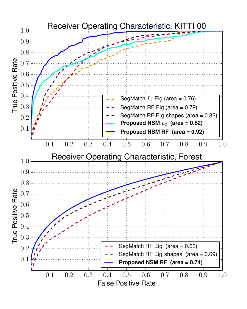
Figure 6: Receiver Operator Characteristic curves for NSM and SegMatch [2] evaluated on Seq 00 of the KITTI dataset (top) and a forest dataset, similar to GS (bottom). The proposed approach was evaluated with both k-NN in feature space ($L_{2}$, cyan) and a pre-trained Random Forest (RF) classifiers (blue). The baseline was evaluated with Eigenvalue-based (Eig) features and Eigenvalue with ESH (Eig_shapes) features.

The choice of evaluation metric is motivated by [4].

The following three experiments were carried out to support our claims:

1. Quantitative analysis of the performance of the proposed hybrid feature descriptor on urban and forested data with comparison to the baseline.

2. Both qualitative and quantitative evaluation of our method performing in parkland environment, showing that the extracted segments are better represented by the oriented key pose resulting in more accurate localizations.

3. A demonstration of the performance of our localization system in a very heavily vegetated environment.

A video to accompany this paper is available at
http://ori.ox.ac.uk/nsm-localization.

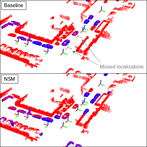
Figure 7: Qualitative illustration of the performance of our algorithm (bottom) on the KITTI dataset in comparison to the baseline (top). Blue point clouds represent correctly identified segments in the source cloud (red). Axis-colored poses indicate successful localizations, while grey colored are missed localizations.

IV-A Feature Description Analysis

The first experiment examines the performance of our hybrid feature descriptor. We use an approach similar to that presented in [2]. We use the KITTI dataset and a forested environment similar to the GS dataset. The KITTI dataset was captured by a 3D Velodyne HDL-64E LIDAR mounted on a car in an urban environment. The forested dataset was recorded with a 3D Velodyne VLP-16 mounted on top of a Clearpath Robotics Husky UGV, as shown in Fig. 5.

Fig. 6 (top) illustrates the Receiver Operating Characteristic (ROC) curves for three combinations of features and two classifiers. Namely, we compared Eigenvalue-based features and Ensemble of Shape Histogram (ESH) features, as proposed in [2] to our hybrid feature extractor. Furthermore, we compared the performance of a RF classifier trained on the aforementioned features to the $L_{2}$ distance in feature space (k-NN). Our proposed approach extracted more positive matches than the baseline with both $L_{2}$ distance in feature space (cyan in comparison to dashed orange) and a RF classifier (blue compared to dashed brown), while limiting false positive correspondences. In the illustrative example on Fig. 7, we show that the proposed approach was able to produce two more localizations as it successfully matched partial observations of segments from the front on the vehicle (bottom of Fig. 7).

Fig. 6 (bottom) illustrates the ROC curve of the proposed features’ classifier against the baseline on the forest dataset. The performance of the all the classifiers is significantly lower than on the urban dataset. The proposed feature extraction method has larger area under the curve (AUC) compared to the baseline. This result could be improved by learning features, optimized for specific environments. We plan to explore this topic in our future work.

Based on these results, we chose a false positive rate of 0.1 (RF score $w=0.69$) for our subsequent experiments in order to limit false positive segment matches and maximize performance.

Figure 8: Translation (top) and rotation (bottom) errors for the proposed approach (continuous lines) and the baseline algorithm (dashed lines) tested on the GS dataset from two sequential runs. Run 1 was used to create the map.

IV-B Performance in a Parkland Environment

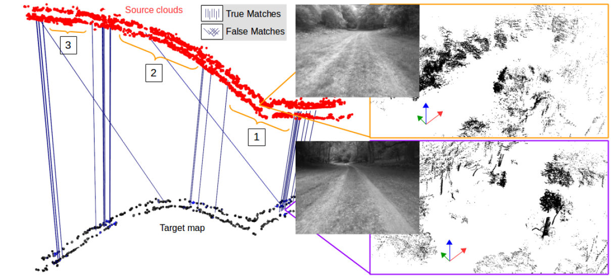
Figure 9: Illustration of the proposed approach on the GS dataset (left) and CP dataset (right). In both environments the source clouds (red) are being registered to an a-priori target map (black). An example of a point cloud during successful localization in the presence of trees is shown in purple, while an example of a missed localization (observed in 1, 2, 3) in the absence of rigid objects is illustrated in orange. Images from the robot’s point of view are shown to illustrate the challenging scenario.

		Transl RMSE	Rot RMSE	Localizations	Frames
	Run 2	$0.43\text{m}\pm 0.22\text{m}$	$2.22^{\circ}\pm 1.03^{\circ}$	$\mathbf{16}$	${26}$
SegMatch	Run 3	$0.37\text{m}\pm 0.25\text{m}$	$2.28^{\circ}\pm 1.45^{\circ}$	$8$	${29}$
	Run 2	$\mathbf{0.22m}\pm\mathbf{0.11m}$	$\mathbf{1.35}^{\circ}\pm\mathbf{0.76}^{\circ}$	$\mathbf{16}$	${26}$
NSM	Run 3	$\mathbf{0.22m}\pm\mathbf{0.09m}$	$\mathbf{1.12}^{\circ}\pm\mathbf{0.67}^{\circ}$	$\mathbf{9}$	${29}$

TABLE III: Quantitative results of the proposed approach and the baseline on GS dataset.

In a second experiment we aim to showcase the proposed key pose selection strategy of our system in a park environment. It consists of well-observed trees, benches and bushes spatially separated and with few interleaved branches between the trees.

This experiment was carried out in George Square Park, Edinburgh, with a Clearpath Husky robot (Fig. 5, left) traversing three loops of $\sim 500\text{m}$ each. The first loop was used to create the map (Run 1), while loops two and three (Run 2, 3) were used to test the localization. The vehicle was equipped with a push-broom LIDAR. Visual odometry [17] was used to create 3D LIDAR swathes for both the prior map and the source clouds. The prior map was further corrected in a SLAM system using [18] by carefully identifying loop closures. For the source cloud, LIDAR swathes were accumulated every $\sim 10\text{m}$ that the vehicle travelled. To account for the different sensor classes the segmentation algorithm parameters were changed as listed in Tab. II. In this experiment we compared NSM to the baseline using centroid computation, Eigenvalue features and the RF classifier. Note that we tried utilising Eigenvalue+ESH features with a pre-trained RF, however, no localization proposals were produced with this system configuration.

Fig. 8 illustrates translation and rotation error as computed using Eq. (4) from the last two test runs. A visual representation of the environment and a running example of it are shown on Fig. 9 (left). Neither the baseline, nor the proposed approach produced any false localizations. Quantitative results of the experiment are shown in Tab. III. The proposed approach shows better accuracy for localization. We speculate that in the case of NSM the oriented key pose extraction strategy contributes for a closer match to the ground truth estimate, as previously illustrated on Fig. 3.

IV-C Performance in a Foliage-Heavy Forest

The last experiment demonstrates the potential of our system to localize in highly vegetated scenes. The data for the experiment was collected in Cornbury Park, Oxfordshire, while traversing an approximately $1\text{km}$ path through woodland. The data was captured by a Bowler Wildcat equipped with a Velodyne HDL-32E LIDAR, producing 3D point cloud scans at 10Hz (Fig. 5, right). Pictures from a camera mounted on a robot in this environment are shown in Fig. 9 (right). This environment was very challenging to localize in, even for a person manually comparing the prior map to a source point cloud. It consists of heavily interleaved foliage, trees and bushes without clear spatial separation.

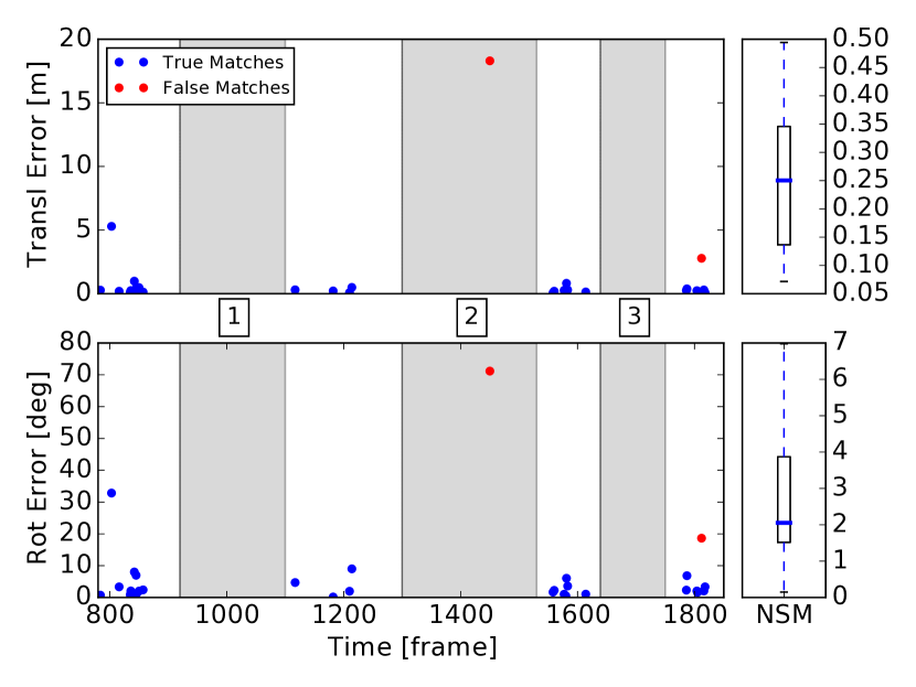
Figure 10: 3D translation error (top) and rotation error (bottom) of correct and incorrect localizations, evaluated on the CP dataset. True matches (blue) correspond to the consistent vertical lines in Fig. 9 (right), while incorrect localizations (red), correspond to inconsistent diagonal lines in Fig. 9 (right). Boxplots on the right indicate the quantiles for the distribution of 0.50 (thick blue bars), 0.25 and 0.75 (lower and upper black rectangles) of true localization matches. During the experiment the vehicle traversed areas of continuous vegetation (1, 2, 3).

Because the vehicle was equipped with a combined GPS/INS sensor, we intended to use this for evaluation. However, the route along the path combined periods of GPS reception and periods where trees covered the path and blocked GPS reception. Instead, we created the map by combining an initial vehicle trajectory, made by registering scans spaced every $30\text{m}$ to one another using ICP, with carefully chosen and reliable GPS measurements. To do this we smoothed the initial trajectory with the GPS measurements using [18] to achieve a best estimate of ground truth. Source point clouds were created when traversing the environment in the opposite direction by accumulating point clouds for every $\sim 1\,\text{m}$ travelled.

Fig. 10 presents the translation and rotation errors of correct and incorrect localization matches, computed using Eq. (4). In the environment we discovered three sections of uninterrupted bushes obscuring any trees (marked with 1, 2, 3 on Fig. 10 and Fig. 9, right). In these areas we did not expect the algorithm to function, as the continuous hedge was visually challenging even for a person to distinguish. Outside these areas there were $96.7\%$ positive and $3.32\%$ false localization matches. We envisage that the two false detections were due to the radius of the Gestalt feature, as this feature’s descriptiveness depends on the size and symmetry of the objects. In those specific cases two small bushes, with boundary points of their convex hull equal to the Gestalt radius, were incorrectly matched to bigger bushes that fully encapsulated them.

In this environment the descriptiveness of the features enabled the proposed approach to produce a series of successful localizations. This was achieved by identifying partially observed and asymmetrical segments.

V Discussion and Limitations

As described above the proposed approach is able to provide reliable localization proposals in urban and natural environments without specific parameter tuning, despite encountering challenging vegetated scenes. The current limitations of the algorithm are:

1. The segmentation of large objects can differ between the target map and the current point cloud when the sensor vantage point changes significantly. This would result in dissimilar segments which could not be matched.

2. The Gestalt descriptor has bins of varying sizes and the descriptor’s azimuthal divisions intersect near the key pose. Thus, the feature descriptor is vulnerable to the precise location of the key pose.

3. There are no constraints on the location of the segments with respect to the vehicle, which influences the way RANSAC estimates a registration. In forests and orchards the simple regularity can cause the step to struggle such as in frame 803 of Exp. C (Fig. 10), where the error is noticeably higher than the RMSE. This is still considered as a true localization (blue dot $\approx 5\,m$ RMSE and $30^{\circ}$ rotation error), as the segments are matched correctly but the precise alignment was incorrect due to all the segments being located on one side of the vehicle. This will be addressed in our future work.

VI Conclusion and Future work

In this paper, we presented Natural Segmentation and Matching, a novel approach for feature description and matching for global localization in natural and urban environments. Our method exploits rigid objects which are repeatable and distinctive in unstructured scenes which allows us to successfully recognize previously visited places. We implemented our approach and evaluated it on an urban, park, and heavily vegetated datasets. The experiments demonstrated that NSM performs comparably to state-of-the-art approaches in an urban environment, while also outperforming these algorithms in natural environments without specific parameter tuning.

In future plans we aim to extend the algorithm to learn environment specific features and to perform multi-seasonal evaluation.

VII Acknowledgement

We would like to thank the authors of SegMatch [2] for open sourcing their implementation and sharing valuable insights about it.

References

- [1] Michael Bosse and Robert Zlot. Place recognition using keypoint voting in large 3D LIDAR datasets. In IEEE Intl. Conf. on Robotics and Automation (ICRA), pages 2677–2684. IEEE, 2013.
- [2] Renaud Dubé, Daniel Dugas, Elena Stumm, Juan Nieto, Roland Siegwart, and Cesar C. Lerma. SegMatch: Segment based place recognition in 3D point clouds. In IEEE Intl. Conf. on Robotics and Automation (ICRA), pages 5266–5272, 2017.
- [3] Gil Elbaz, Tamar Avraham, and Anath Fischer. 3D Point Cloud Registration for Localization using a Deep Neural Network Auto-Encoder. In Proc. IEEE Int. Conf. Computer Vision and Pattern Recognition, pages 2472–2481, 2017.
- [4] François Pomerleau, Francis Colas, Roland Siegwart, and Stéphane Magnenat. Comparing ICP variants on real-world data sets. Autonomous Robots, 34(3):133–148, April 2013.
- [5] Jacopo Serafin and Giorgio Grisetti. NICP: Dense normal based point cloud registration. In IEEE/RSJ Intl. Conf. on Intelligent Robots and Systems (IROS), pages 742–749, Sept 2015.
- [6] Carl Wellington, Joan Campoy, Lav Khot, and Reza Ehsani. Orchard tree modeling for advanced sprayer control and automatic tree inventory. In IEEE/Intl. Conf. on Computer Vision Workshops (ICCV Workshops), pages 5–6, 2012.
- [7] James P Underwood, Gustav Jagbrant, Juan I Nieto, and Salah Sukkarieh. LIDAR-based tree recognition and platform localization in orchards. J. of Field Robotics, 32(8):1056–1074, 2015.
- [8] Michael Bosse and Robert Zlot. Keypoint design and evaluation for place recognition in 2D LIDAR maps. Journal of Robotics and Autonomous Systems, 57(12):1211–1224, 2009.
- [9] Michael Bosse and Robert Zlot. Place recognition using regional point descriptors for 3D mapping. In Field and Service Robotics, pages 195–204. Springer, 2010.
- [10] Paul J. Besl and Neil D. McKay. A method for registration of 3-D shapes. IEEE Trans. Pattern Anal. Machine Intell., 14(2):239–256, February 1992.
- [11] Lawrence R Rabiner. A tutorial on Hidden Markov Models and selected applications in speech recognition. Proc. of the IEEE, 77(2):257–286, 1989.
- [12] Keqi Zhang, Shu-Ching Chen, Dean Whitman, Mei-Ling Shyu, Jianhua Yan, and Chengcui Zhang. A progressive morphological filter for removing nonground measurements from airborne LIDAR data. IEEE Transactions on Geoscience and Remote Sensing, 41(4):872–882, 2003.
- [13] Tahir Rabbani, Frank Van Den Heuvel, and George Vosselmann. Segmentation of point clouds using smoothness constraint. ISPRS Annals of the Phot., Remote Sens. and Spatial Inf. Sciences, 36(5):248–253, 2006.
- [14] Alex Walthelm. Enhancing global pose estimation with laser range scans using local techniques. In Intl. Conf. on Intelligent Autonomous Systems (ICIAS), 2004.
- [15] Aitor Aldoma, Federico Tombari, Luigi Di Stefano, and Markus Vincze. A global hypotheses verification method for 3D object recognition. Eur. Conf. on Computer Vision (ECCV), pages 511–524, 2012.
- [16] Andreas Geiger, Philip Lenz, Christoph Stiller, and Raquel Urtasun. Vision meets robotics: The KITTI dataset. Intl. J. of Robotics Research, 32(11):1231–1237, 2013.
- [17] Albert S. Huang, Abraham Bachrach, Peter Henry, Michael Krainin, Daniel Maturana, Dieter Fox, and Nicholas Roy. Visual Odometry and Mapping for Autonomous Flight Using an RGB-D camera. In Intl. J. of Robotics Research, pages 235–252. Springer, 2017.
- [18] Michael Kaess, Ananth Ranganathan, and Frank Dellaert. iSAM: Incremental Smoothing and Mapping. IEEE Trans. Robotics, 24(6):1365–1378, 2008.