Fully-Functional Suffix Trees and Optimal Text Searching
in BWT-runs Bounded Space

Abstract

Indexing highly repetitive texts — such as genomic databases, software repositories and versioned text collections — has become an important problem since the turn of the millennium. A relevant compressibility measure for repetitive texts is $r$, the number of runs in their Burrows-Wheeler Transforms (BWTs). One of the earliest indexes for repetitive collections, the Run-Length FM-index, used $O(r)$ space and was able to efficiently count the number of occurrences of a pattern of length $m$ in the text (in loglogarithmic time per pattern symbol, with current techniques). However, it was unable to locate the positions of those occurrences efficiently within a space bounded in terms of $r$. Since then, a number of other indexes with space bounded by other measures of repetitiveness — the number of phrases in the Lempel-Ziv parse, the size of the smallest grammar generating (only) the text, the size of the smallest automaton recognizing the text factors — have been proposed for efficiently locating, but not directly counting, the occurrences of a pattern. In this paper we close this long-standing problem, showing how to extend the Run-Length FM-index so that it can locate the $occ$ occurrences efficiently within $O(r)$ space (in loglogarithmic time each), and reaching optimal time, $O(m+occ)$, within $O(r\log\log_{w}(\sigma+n/r))$ space, for a text of length $n$ over an alphabet of size $\sigma$ on a RAM machine with words of $w=\Omega(\log n)$ bits. Within that space, our index can also count in optimal time, $O(m)$. Multiplying the space by $O(w/\log\sigma)$, we support count and locate in $O(\lceil m\log(\sigma)/w\rceil)$ and $O(\lceil m\log(\sigma)/w\rceil+occ)$ time, which is optimal in the packed setting and had not been obtained before in compressed space. We also describe a structure using $O(r\log(n/r))$ space that replaces the text and extracts any text substring of length $\ell$ in almost-optimal time $O(\log(n/r)+\ell\log(\sigma)/w)$. Within that space, we similarly provide direct access to suffix array, inverse suffix array, and longest common prefix array cells, and extend these capabilities to full suffix tree functionality, typically in $O(\log(n/r))$ time per operation. Our experiments show that our $O(r)$-space index outperforms the space-competitive alternatives by 1–2 orders of magnitude.

1 Introduction

The data deluge has become a pervasive problem in most organizations that aim to collect and process data. We are concerned about string (or text, or sequence) data, formed by collections of symbol sequences. This includes natural language text collections, DNA and protein sequences, source code repositories, semistructured text, and many others. The rate at which those sequence collections are growing is daunting, in some cases outpacing Moore’s Law by a significant margin [109]. A key to handle this growth is the fact that the amount of unique material does not grow at the same pace of the sequences. Indeed, the fastest-growing string collections are in many cases highly repetitive, that is, most of the strings can be obtained from others with a few modifications. For example, most genome sequence collections store many genomes from the same species, which in the case of, say, humans differ by 0.1% [102] (there is some discussion about the exact percentage). The 1000-genomes project uses a Lempel-Ziv-like compression mechanism that reports compression ratios around 1% [40] (i.e., the compressed space is about two orders of magnitude less than the uncompressed space). Versioned document collections and software repositories are another natural source of repetitiveness. For example, Wikipedia reports that, by June 2015, there were over 20 revisions (i.e., versions) per article in its 10 TB content, and that p7zip compressed it to about 1%. They also report that what grows the fastest today are the revisions rather than the new articles, which increases repetitiveness. A study of GitHub (which surpassed 20 TB in 2016) reports a ratio of commit (new versions) over create (brand new projects) around 20.

Version management systems offer a good solution to the problem of providing efficient access to the documents of a versioned collection, at least when the versioning structure is known. They factor out repetitiveness by storing the first version of a document in plain form and then the edits of each version of it. It is much more challenging, however, to provide more advanced functionalities, such as counting or locating the positions where a string pattern occurs across the collection.

An application field where this need is most pressing is bioinformatics. The FM-index [32, 33] was extremely successful in reducing the size of classical data structures for pattern searching, such as suffix trees [114] or suffix arrays [81], to the statistical entropy of the sequence while emulating a significant part of their functionality. The FM-index has had a surprising impact far beyond the boundaries of theoretical computer science: if someone now sends his or her genome to be analyzed, it will almost certainly be sequenced on a machine built by Illumina, which will produce a huge collection of quite short substrings of that genome, called reads. Those reads’ closest matches will then be sought in a reference genome, to determine where they most likely came from in the newly-sequenced target genome, and finally a list of the likely differences between the target and the reference genomes will be reported. The searches in the reference genome will be done almost certainly using software such as Bowtie, BWA, or Soap2, all of them based on the FM-index.

Genomic analysis is already an important field of research, and a rapidly growing industry [107]. As a result of dramatic advances in sequencing technology, we now have datasets of tens of thousands of genomes, and bigger ones are on their way (e.g., there is already a 100,000-human-genomes project).  Unfortunately, current software based on FM-indexes cannot handle such massive datasets: they use 2 bits per base at the very least [65]. Even though the FM-index can represent the sequences within their statistical entropy [33], this measure is insensitive to the repetitiveness of those datasets [73, Lem. 2.6], and thus the FM-indexes would grow proportionally to the sizes of the sequences. Using current tools, indexing a set of 100,000 human genomes would require 75 TB of storage at the very least, and the index would have to reside in main memory to operate efficiently. To handle such a challenge we need, instead, compressed text indexes whose size is proportional to the amount of unique material in those huge datasets.

1.1 Related work

Mäkinen et al. [78, 108, 79, 80] pioneered the research on indexing and searching repetitive collections. They regard the collection as a single concatenated text $T[1..n]$ with separator symbols, and note that the number $r$ of runs (i.e., maximal substrings formed by a single symbol) in the Burrows-Wheeler Transform [20] of the text is relatively very low on repetitive texts. Their index, Run-Length FM-Index (RLFM-index), uses $O(r)$ words and can count the number of occurrences of a pattern $P[1..m]$ in time $O(m\log n)$ and even less. However, they are unable to locate where those positions are in $T$ unless they add a set of samples that require $\Theta(n/s)$ words in order to offer $O(s\log n)$ time to locate each occurrence. On repetitive texts, either this sampled structure is orders of magnitude larger than the $O(r)$-size basic index, or the locating time is extremely high.

Many proposals since then aimed at reducing the locating time by building on other compression methods that perform well on repetitive texts: indexes based on the Lempel-Ziv parse [76] of $T$, with size bounded in terms of the number $z$ of phrases [73, 42, 97, 9, 88, 15, 23]; indexes based on the smallest context-free grammar (or an approximation thereof) that generates $T$ and only $T$ [68, 21], with size bounded in terms of the size $g$ of the grammar [25, 26, 41, 89]; and indexes based on the size $e$ of the smallest automaton (CDAWG) [18] recognizing the substrings of $T$ [9, 111, 7]. Table 1 summarizes the pareto-optimal achievements. We do not consider in this paper indexes based on other repetitiveness measures that only apply in restricted scenarios, such as those based on Relative Lempel-Ziv [74, 27, 11, 29] or on alignments [86, 87].

Index	Space	Count time
Navarro [89, Thm. 6]	$O(z\log(n/z))$	$O(m\log n+m\log^{2+\epsilon}(n/z))$
Navarro [89, Thm. 5]	$O(g)$	$O(m^{2}+m\log^{2+\epsilon}g)$
Mäkinen et al. [80, Thm. 17]	$O(r)$	$O(m(\frac{\log\sigma}{\log\log r}+(\log\log n)^{2}))$
This paper (Lem. 1)	$O(r)$	$O(m\log\log_{w}(\sigma+n/r))$
This paper (Thm. 4.1)	$O(r\log\log_{w}(\sigma+n/r))$	$O(m)$
This paper (Thm. 4.2)	$O(rw\log_{\sigma}\log_{w}(\sigma+n/r))$	$O(\lceil m\log(\sigma)/w\rceil)$

Index	Space	Locate time
Kreft and Navarro [73, Thm. 4.11]	$O(z)$	$O(m^{2}h+(m+occ)\log z)$
Gagie et al. [42, Thm. 4]	$O(z\log(n/z))$	$O(m\log m+occ\log\log n)$
Bille et al. [15, Thm. 1]	$O(z\log(n/z))$	$O(m(1+\log^{\epsilon}z/\log(n/z))+occ(\log^{\epsilon}z+\log\log n))$
Christiansen and Ettienne [23, Thm. 2(3)]	$O(z\log(n/z))$	$O(m+\log^{\epsilon}z+occ(\log^{\epsilon}z+\log\log n))$
Christiansen and Ettienne [23, Thm. 2(1)]	$O(z\log(n/z)+z\log\log z)$	$O(m+occ(\log^{\epsilon}z+\log\log n))$
Bille et al. [15, Thm. 1]	$O(z\log(n/z)\log\log z)$	$O(m+occ\log\log n)$
Claude and Navarro [26, Thm. 1]	$O(g)$	$O(m^{2}\log\log_{g}n+(m+occ)\log g)$
Gagie et al. [41, Thm. 4]	$O(g+z\log\log z)$	$O(m^{2}+(m+occ)\log\log n)$
Mäkinen et al. [80, Thm. 20]	$O(r+n/s)$	$O((m+s\cdot occ)(\frac{\log\sigma}{\log\log r}+(\log\log n)^{2}))$
Belazzougui et al. [9, Thm. 3]	$O(\overline{r}+z)$	$O(m(\log z+\log\log n)+occ(\log^{\epsilon}z+\log\log n))$
This paper (Thm. 3.1)	$O(r)$	$O((m+occ)\log\log_{w}(\sigma+n/r))$
This paper (Thm. 4.1)	$O(r\log\log_{w}(\sigma+n/r))$	$O(m+occ)$
This paper (Thm. 4.2)	$O(rw\log_{\sigma}\log_{w}(\sigma+n/r))$	$O(\lceil m\log(\sigma)/w\rceil+occ)$
Belazzougui and Cunial [7, Thm. 1]	$O(e)$	$O(m+occ)$

Structure	Space	Extract time
Kreft and Navarro [73, Thm. 4.11]	$O(z)$	$O(\ell\,h)$
Gagie et al. [10, Thm. 2]	$O(z\log(n/z))$	$O((1+\ell/\log_{\sigma}n)\log(n/z))$
Belazzougui et al. [14, Thm. 1]	$O(g)$	$O(\log n+\ell/\log_{\sigma}n)$
Belazzougui et al. [14, Thm. 2]	$O(g\log^{\epsilon}n\log(n/g))$	$O(\log n/\log\log n+\ell/\log_{\sigma}n)$
Mäkinen et al. [80, Thm. 20]	$O(r+n/s)$	$O((s+\ell)(\frac{\log\sigma}{\log\log r}+(\log\log n)^{2}))$
This paper (Thm. 5.1)	$O(r\log(n/r))$	$O(\log(n/r)+\ell\log(\sigma)/w)$
Belazzougui and Cunial [7, Thm. 1]	$O(e)$	$O(\log n+\ell)$

Structure	Space	Typical suffix tree operation time
Mäkinen et al. [80, Thm. 30]	$O(r+n/s)$	$O(s(\frac{\log\sigma}{\log\log r}+(\log\log n)^{2}))$
This paper (Thm. 6.1)	$O(r\log(n/r))$	$O(\log(n/r))$
Belazzougui and Cunial [8, Thm. 1]	$O(\overline{e})$	$O(\log n)$

Table 1: Previous and our new results on counting, locating, extracting, and supporting suffix tree functionality. We simplified some formulas with tight upper bounds. The variables are the text size $n$, pattern length $m$, number of occurrences $occ$ of the pattern, alphabet size $\sigma$, extracted length $\ell$, Lempel-Ziv parsing size $z$, smallest grammar size $g$, $\mathit{BWT}$ runs $r$, CDAWG size $e$, and machine word length in bits $w$. Variable $h\leq z$ is the depth of the dependency chain in the Lempel-Ziv parse, and $\epsilon>0$ is an arbitrarily small constant. Symbols $\overline{r}$ or $\overline{e}$ mean $r$ or $e$ of $T$ plus $r$ or $e$ of its reverse. The $z$ of Kreft and Navarro [73] refers to the Lempel-Ziv variant that does not allow overlaps between sources and targets, but their index actually works in either variant.

There are a few known asymptotic bounds between the repetitiveness measures $r$, $z$, $g$, and $e$: $z\leq g=O(z\log(n/z))$ [105, 21, 58] and $e=\Omega(\max(r,z,g))$ [9, 8]. Examples of string families are known that show that $r$ is not comparable with $z$ and $g$ [9, 101]. Experimental results [80, 73, 9, 24], on the other hand, suggest that in typical repetitive texts it holds $z<r\approx g\ll e$.

For highly repetitive texts, one hopes to have a compressed index not only able to count and locate pattern occurrences, but also to replace the text with a compressed version that nonetheless can efficiently extract any substring $T[i..i+\ell]$. Indexes that, implicitly or not, contain a replacement of $T$, are called self-indexes. As can be seen in Table 1, self-indexes with $O(z)$ space require up to $O(z)$ time per extracted character, and none exists within $O(r)$ space. Good extraction times are instead obtained with $O(g)$, $O(z\log(n/z))$, or $O(e)$ space. A lower bound for grammar-based representations [113] shows that $\Omega((\log n)^{1-\epsilon}/\log g)$ time, for any constant $\epsilon>0$, is needed to access one random position within $O(\mathrm{poly}(g))$ space. This bound shows that various current techniques using structures bounded in terms of $g$ or $z$ [17, 14, 43, 10] are nearly optimal (note that $g=\Omega(\log n)$, so the space of all these structures is $O(\mathrm{poly}(g))$). In an extended article [22, Thm. 6], the authors give a lower bound in terms of $r$, for binary texts on a RAM machine of $w=\Theta(\log n)$ bits: $\Omega((\log n)^{1-\epsilon})$ for some constant $\epsilon$ when using $O(\mathrm{poly}(r\log n))$ space.

In more sophisticated applications, especially in bioinformatics, it is desirable to support a more complex set of operations, which constitute a full suffix tree functionality [54, 98, 77]. While Mäkinen et al. [80] offered suffix tree functionality, they had the same problem of needing $\Theta(n/s)$ space to achieve $O(s\log n)$ time for most suffix tree operations. Only recently a suffix tree of size $O(\overline{e})$ supports most operations in time $O(\log n)$ [9, 8], where $\overline{e}$ refers to the $e$ measure of $T$ plus that of $T$ reversed.

Summarizing Table 1 and our discussion, the situation on repetitive text indexing is as follows.

1. The RLFM-index is the only structure able to count the occurrences of $P$ in $T$ in time $O(m\log n)$. However, it does not offer efficient locating within $O(r)$ space.

2. The only structure clearly smaller than the RLFM-index, using $O(z)$ space [73], has unbounded locate time. Structures using about the same space, $O(g)$, have an $\Omega(m^{2})$ one-time overhead in the locate time [25, 26, 41, 89].

3. Structures offering lower locate times require $\Omega(z\log(n/z))$ space [42, 97, 15, 23, 89], $\Theta(\overline{r}+z)$ space [9] (where $\overline{r}$ is the sum of $r$ for $T$ and its reverse), or $\Omega(e)$ space [9, 111, 7].

4. Self-indexes with efficient extraction require $\Omega(z\log(n/z))$ space [105, 21, 43, 10, 15], $\Omega(g)$ space [17, 14], or $\Omega(e)$ space [111, 7].

5. The only efficient compressed suffix tree requires $\Theta(\overline{e})$ space [8].

6. Only a few of all these indexes have been implemented, as far as we know [80, 25, 73, 9].

1.2 Contributions

Efficiently locating the occurrences of $P$ in $T$ within $O(r)$ space has been a bottleneck and an open problem for almost a decade. In this paper we give the first solution to this problem. Our precise contributions, largely detailed in Tables 1 and 2, are the following:

1. We improve the counting time of the RLFM-index to $O(m\log\log_{w}(\sigma+n/r))$, where $\sigma\leq r$ is the alphabet size of $T$, while retaining the $O(r)$ space.

2. We show how to locate each occurrence in time $O(\log\log_{w}(n/r))$, within $O(r)$ space. We reduce the locate time to $O(1)$ per occurrence by using slightly more space, $O(r\log\log_{w}(n/r))$.

3. By using $O(r\log\log_{w}(\sigma+n/r))$ space, we obtain optimal locate time in the general setting, $O(m+occ)$, as well as optimal counting time, $O(m)$. This had been obtained before only with space bounds $O(e)$ [7] or $O(\overline{e})$ [111].

4. By increasing the space to $O(rw\log_{\sigma}\log_{w}(\sigma+n/r))$, we obtain optimal locate time, $O(\lceil m\log(\sigma)/w\rceil+occ)$, and optimal counting time, $O(\lceil m\log(\sigma)/w\rceil)$, in the packed setting (i.e., the pattern symbols come packed in blocks of $w/\log\sigma$ symbols per word). This had not been achieved so far by any compressed index, but only by uncompressed ones [91].

5. We give the first structure built on $\mathit{BWT}$ runs that replaces $T$ while retaining direct access. It extracts any substring of length $\ell$ in time $O(\log(n/r)+\ell\log(\sigma)/w)$, using $O(r\log(n/r))$ space. As discussed, even the additive penalty is near-optimal [22, Thm. 6]. Within the same space, we also obtain optimal locating and counting time, as well as accessing subarrays of length $\ell$ of the suffix array, inverse suffix array, and longest common prefix array of $T$, in time $O(\log(n/r)+\ell)$.

6. We give the first compressed suffix tree whose space is bounded in terms of $r$, $O(r\log(n/r))$ words. It implements most navigation operations in time $O(\log(n/r))$. There exist only comparable suffix trees within $O(\overline{e})$ space [8], taking $O(\log n)$ time for most operations.

7. We provide a proof-of-concept implementation of the most basic index (the one locating within $O(r)$ space), and show that it outperforms all the other implemented alternatives by orders of magnitude in space or in time to locate pattern occurrences.

Functionality	Space (words)	Time
Count $+$ Locate (Thm. 3.1)	$O(r)$	$O(m\log\log_{w}(\sigma+n/r)+occ\log\log_{w}(n/r))$
Count $+$ Locate (Lem. 4)	$O(r\log\log_{w}(n/r))$	$O(m\log\log_{w}(\sigma+n/r)+occ)$
Count $+$ Locate (Thm. 4.1)	$O(r\log\log_{w}(\sigma+n/r))$	$O(m+occ)$
Count $+$ Locate (Thm. 4.2)	$O(rw\log_{\sigma}\log_{w}(\sigma+n/r))$	$O(\lceil m\log(\sigma)/w\rceil+occ)$
Extract (Thm. 5.1)	$O(r\log(n/r))$	$O(\log(n/r)+\ell\log(\sigma)/w)$
Access $\mathit{SA}$, $\mathit{ISA}$, $\mathit{LCP}$ (Thm. 5.2–5.4)	$O(r\log(n/r))$	$O(\log(n/r)+\ell)$
Count $+$ Locate (Thm. 5.5)	$O(r\log(n/r))$	$O(m+occ)$
Suffix tree (Thm. 6.1)	$O(r\log(n/r))$	$O(\log(n/r))$ for most operations

Table 2: Our contributions. For any “Count $+$ Locate”, we can do only “Count” in the time given by setting $occ=0$.

Contribution 1 is a simple update of the RLFM-index [80] with newer data structures for rank and predecessor queries [13]. We present it in Section 2, together with a review of the basic concepts needed to follow the paper.

Contribution 2 is one of the central parts of the paper, and is obtained in Section 3 in two steps. The first uses the fact that we can carry out the classical RLFM-index counting process for $P$ in a way that we always know the position of one occurrence in $T$ [101, 100]; we give a simpler proof of this fact in Lemma 2. The second shows that, if we know the position in $T$ of one occurrence of $\mathit{BWT}$, then we can quickly obtain the preceding and following ones with an $O(r)$-size sampling. This is achieved by using the $\mathit{BWT}$ runs to induce phrases in $T$ (which are somewhat analogous to the Lempel-Ziv phrases [76]) and showing that the positions of occurrences within phrases can be obtained from the positions of their preceding phrase start. The time $O(1)$ is obtained by using an extended sampling.

For Contributions 3 and 4, we use in Section 4 the fact that the RLFM-index on a text regarded as a sequence of overlapping metasymbols of length $s$ has at most $rs$ runs, so that we can process the pattern by chunks of $s$ symbols. The optimal packed time is obtained by enlarging the samplings.

In Section 5, Contribution 5 uses an analogue of the Block Tree [10] built on the $\mathit{BWT}$-induced phrases, which satisfies the property that any distinct string has an occurrence overlapping a border between phrases. Further, it is shown that direct access to the suffix array $\mathit{SA}$, inverse suffix array $\mathit{ISA}$, and array $\mathit{LCP}$ of $T$, can be supported in a similar way because they inherit the same repetitiveness properties of the text.

Contribution 6 needs, in addition to accessing those arrays, some sophisticated operations on the $\mathit{LCP}$ array [37] that are not well supported by Block Trees. In Section 6, we implement suffix trees by showing that a run-length context-free grammar [NIIBT16] of size $O(r\log(n/r))$ can be built on the differential $\mathit{LCP}$ array, and then implement the required operations on it.

The results of Contribution 7 are shown in Section 7. Our experimental results show that our simple $O(r)$-space index outperforms the alternatives by orders of magnitude when locating the occurrences of a pattern, while being simultaneously smaller or nearly as small. The only compact structure outperforming our index, the CDAWG, is an order of magnitude larger.

Further, in Section 8 we describe construction algorithms for all our data structures, achieving construction spaces bounded in terms of $r$ for the simpler and most practical structures. We finally conclude in Section 9.

This article is an extension of a conference version presented in SODA 2018 [46]. The extension consists, on the one hand, in a significant improvement in Contributions 3 and 4: in Section 4, optimal time locating is now obtained in a much simpler way and in significantly less space. Further, optimal time is obtained as well, which is new. On the other hand, Contribution 6, that is, the machinery to support suffix tree functionality in Section 6, is new. We also present an improved implementation in Section 7, with better experimental results. Finally, the construction algorithms in Section 8 are new as well.

2 Basic Concepts

A string is a sequence $S[1..\ell]=S[1]S[2]\ldots S[\ell]$, of length $\ell=|S|$, of symbols (or characters, or letters) chosen from an alphabet $[1..\sigma]=\{1,2,\ldots,\sigma\}$, that is, $S[i]\in[1..\sigma]$ for all $1\leq i\leq\ell$. We use $S[i..j]=S[i]\ldots S[j]$, with $1\leq i,j\leq\ell$, to denote a substring of $S$, which is the empty string $\varepsilon$ if $i>j$. A prefix of $S$ is a substring of the form $S[1..i]$ (also written $S[..i]$) and a suffix is a substring of the form $S[i..\ell]$ (also written $S[i..]$). The juxtaposition of strings and/or symbols represents their concatenation.

We will consider indexing a text $T[1..n]$, which is a string over alphabet $[1..\sigma]$ terminated by the special symbol $\$=1$, that is, the lexicographically smallest one, which appears only at $T[n]=\$$. This makes any lexicographic comparison between suffixes well defined.

Our computation model is the transdichotomous RAM, with a word of $w=\Omega(\log n)$ bits, where all the standard arithmetic and logic operations can be carried out in constant time. In this article we generally measure space in words.

2.1 Suffix Trees and Arrays

The suffix tree [114] of $T[1..n]$ is a compacted trie where all the $n$ suffixes of $T$ have been inserted. By compacted we mean that chains of degree-1 nodes are collapsed into a single edge that is labeled with the concatenation of the individual symbols labeling the collapsed edges. The suffix tree has $n$ leaves and less than $n$ internal nodes. By representing edge labels with pointers to $T$, the suffix tree uses $O(n)$ space, and can be built in $O(n)$ time [114, 83, 112, 28].

The suffix array [81] of $T[1..n]$ is an array $\mathit{SA}[1..n]$ storing a permutation of $[1..n]$ so that, for all $1\leq p<n$, the suffix $T[\mathit{SA}[p]..]$ is lexicographically smaller than the suffix $T[\mathit{SA}[p+1]..]$. Thus $\mathit{SA}[p]$ is the starting position in $T$ of the $p$th smallest suffix of $T$ in lexicographic order. This can be regarded as an array collecting the leaves of the suffix tree. The suffix array uses $n$ words and can be built in $O(n)$ time without building the suffix tree [69, 70, 61].

All the occurrences of a pattern string $P[1..m]$ in $T$ can be easily spotted in the suffix tree or array. In the suffix tree, we descend from the root matching the successive symbols of $P$ with the strings labeling the edges. If $P$ is in $T$, the symbols of $P$ will be exhausted at a node $v$ or inside an edge leading to a node $v$; this node is called the locus of $P$, and all the $occ$ leaves descending from $v$ are the suffixes starting with $P$, that is, the starting positions of the occurrences of $P$ in $T$. By using perfect hashing to store the first characters of the edge labels descending from each node of $v$, we reach the locus in optimal time $O(m)$ and the space is still $O(n)$. If $P$ comes packed using $w/\log\sigma$ symbols per computer word, we can descend in time $O(\lceil m\log(\sigma)/w\rceil)$ [91], which is optimal in the packed model. In the suffix array, all the suffixes starting with $P$ form a range $\mathit{SA}[sp..ep]$, which can be binary searched in time $O(m\log n)$, or $O(m+\log n)$ with additional structures [81].

The inverse permutation of $\mathit{SA}$, $\mathit{ISA}[1..n]$, is called the inverse suffix array, so that $\mathit{ISA}[i]$ is the lexicographical position of the suffix $T[i..]$ among all the suffixes of $T$.

Another important concept related to suffix arrays and trees is the longest common prefix array. Let $lcp(S,S^{\prime})$ be the length of the longest common prefix between two strings $S\not=S^{\prime}$, that is, $S[1..lcp(S,S^{\prime})]=S^{\prime}[1..lcp(S,S^{\prime})]$ but $S[lcp(S,S^{\prime})+1]\not=S^{\prime}[lcp(S,S^{\prime})+1]$. Then we define the longest common prefix array $\mathit{LCP}[1..n]$ as $\mathit{LCP}[1]=0$ and $\mathit{LCP}[p]=lcp(T[\mathit{SA}[p-1]..],T[\mathit{SA}[p]..])$. The $\mathit{LCP}$ array uses $n$ words and can be built in $O(n)$ time [64].

2.2 Self-indexes

A self-index is a data structure built on $T[1..n]$ that provides at least the following functionality:

Count:

Given a pattern $P[1..m]$, compute the number $occ$ of occurrences of $P$ in $T$.

Locate:

Given a pattern $P[1..m]$, return the $occ$ positions where $P$ occurs in $T$.

Extract:

Given a range $[i..i+\ell-1]$, return $T[i..i+\ell-1]$.

The last operation allows a self-index to act as a replacement of $T$, that is, it is not necessary to store $T$ since any desired substring can be extracted from the self-index. This can be trivially obtained by including a copy of $T$ as a part of the self-index, but it is challenging when the self-index must use little space.

In principle, suffix trees and arrays can be regarded as self-indexes that can count in time $O(m)$ or $O(\lceil m\log(\sigma)/w\rceil)$ (suffix tree, by storing $occ$ in each node $v$) and $O(m\log n)$ or $O(m+\log n)$ (suffix array, with $occ=ep-sp+1$), locate each occurrence in $O(1)$ time, and extract in time $O(\lceil\ell\log(\sigma)/w\rceil)$. However, they use $O(n\log n)$ bits, much more than the $n\log\sigma$ bits needed to represent $T$ in plain form. We are interested in compressed self-indexes [90, 96], which use the space required by a compressed representation of $T$ (under some compressibility measure) plus some redundancy (at worst $o(n\log\sigma)$ bits). We describe later the FM-index, a particular self-index of interest to us.

2.3 Burrows-Wheeler Transform

The Burrows-Wheeler Transform of $T[1..n]$, $\mathit{BWT}[1..n]$ [20], is a string defined as $\mathit{BWT}[p]=T[\mathit{SA}[p]-1]$ if $\mathit{SA}[p]>1$, and $\mathit{BWT}[p]=T[n]=\$$ if $\mathit{SA}[p]=1$. That is, $\mathit{BWT}$ has the same symbols of $T$ in a different order, and is a reversible transform.

The array $\mathit{BWT}$ is obtained from $T$ by first building $\mathit{SA}$, although it can be built directly, in $O(n)$ time and within $O(n\log\sigma)$ bits of space [85]. To obtain $T$ from $\mathit{BWT}$ [20], one considers two arrays, $L[1..n]=\mathit{BWT}$ and $F[1..n]$, which contains all the symbols of $L$ (or $T$) in ascending order. Alternatively, $F[p]=T[\mathit{SA}[p]]$, so $F[p]$ follows $L[p]$ in $T$. We need a function that maps any $L[p]$ to the position $q$ of that same character in $F$. The formula is $\mathit{LF}(p)=C[c]+\mathrm{rank}[p]$, where $c=L[p]$, $C[c]$ is the number of occurrences of symbols less than $c$ in $L$, and $\mathrm{rank}[p]$ is the number of occurrences of symbol $L[p]$ in $L[1..p]$. A simple $O(n)$-time pass on $L$ suffices to compute arrays $C$ and $\mathrm{rank}$ using $O(n\log\sigma)$ bits of space. Once they are computed, we reconstruct $T[n]=\$$ and $T[n-k]\leftarrow L[\mathit{LF}^{k-1}(1)]$ for $k=1,\ldots,n-1$, in $O(n)$ time as well. Note that $\mathit{LF}$ is a permutation formed by a single cycle.

2.4 Compressed Suffix Arrays and FM-indexes

Compressed suffix arrays [90] are a particular case of self-indexes that simulate $\mathit{SA}$ in compressed form. Therefore, they aim to obtain the suffix array range $[sp..ep]$ of $P$, which is sufficient to count since $P$ then appears $occ=ep-sp+1$ times in $T$. For locating, they need to access the content of cells $\mathit{SA}[sp],\ldots,\mathit{SA}[ep]$, without having $\mathit{SA}$ stored.

The FM-index [32, 33] is a compressed suffix array that exploits the relation between the string $L=\mathit{BWT}$ and the suffix array $\mathit{SA}$. It stores $L$ in compressed form (as it can be easily compressed to the high-order empirical entropy of $T$ [82]) and adds sublinear-size data structures to compute (i) any desired position $L[p]$, (ii) the generalized rank function $\mathrm{rank}_{c}(L,p)$, which is the number of times symbol $c$ appears in $L[1..p]$. Note that these two operations permit, in particular, computing $\mathrm{rank}[p]=\mathrm{rank}_{L[p]}(L,p)$, which is called partial rank. Therefore, they compute

$$\mathit{LF}(p)~{}~{}=~{}~{}C[L[p]]+\mathrm{rank}_{L[p]}(L,p).$$

For counting, the FM-index resorts to backward search. This procedure reads $P$ backwards and at any step knows the range $[sp_{j},ep_{j}]$ of $P[j..m]$ in $T$. Initially, we have the range $[sp_{m+1}..ep_{m+1}]=[1..n]$ for $P[m+1..m]=\varepsilon$. Given the range $[sp_{j+1}..ep_{j+1}]$, one obtains the range $[sp_{j}..ep_{j}]$ from $c=P[j]$ with the operations

$$sp_{j} = C[c]+\mathrm{rank}_{c}(L,sp_{j+1}-1)+1,$$

$$ep_{j} = C[c]+\mathrm{rank}_{c}(L,ep_{j+1}).$$

Thus the range $[sp..ep]=[sp_{1}..ep_{1}]$ is obtained with $O(m)$ computations of $\mathrm{rank}$, which dominates the counting complexity.

For locating, the FM-index (and most compressed suffix arrays) stores sampled values of $\mathit{SA}$ at regularly spaced text positions, say multiples of $s$. Thus, to retrieve $\mathit{SA}[p]$, we find the smallest $k$ for which $\mathit{SA}[\mathit{LF}^{k}(p)]$ is sampled, and then the answer is $\mathit{SA}[p]=\mathit{SA}[\mathit{LF}^{k}(p)]+k$. This is because function $\mathit{LF}$ virtually traverses the text backwards, that is, it drives us from $L[p]$, which precedes suffix $\mathit{SA}[p]$, to its position $F[q]$, where the suffix $\mathit{SA}[q]$ starts with $L[p]$, that is, $\mathit{SA}[q]=\mathit{SA}[p]-1$:

$$\mathit{SA}[\mathit{LF}(p)]~{}=~{}\mathit{SA}[p]-1.$$

Since it is guaranteed that $k<s$, each occurrence is located with $s$ accesses to $L$ and computations of $\mathit{LF}$, and the extra space for the sampling is $O((n\log n)/s)$ bits, or $O(n/s)$ words.

For extracting, a similar sampling is used on $\mathit{ISA}$, that is, we sample the positions of $\mathit{ISA}$ that are multiples of $s$. To extract $T[i..i+\ell-1]$ we find the smallest multiple of $s$ in $[i+\ell..n]$, $j=s\cdot\lceil(i+\ell)/s\rceil$, and extract $T[i..j]$. Since $\mathit{ISA}[j]=p$ is sampled, we know that $T[j-1]=L[p]$, $T[j-2]=L[\mathit{LF}(p)]$, and so on. In total we require at most $\ell+s$ accesses to $L$ and computations of $\mathit{LF}$ to extract $T[i..i+\ell-1]$. The extra space is also $O(n/s)$ words.

For example, using a representation [13] that accesses $L$ and computes partial ranks in constant time (so $\mathit{LF}$ is computed in $O(1)$ time), and computes $\mathrm{rank}$ in the optimal $O(\log\log_{w}\sigma)$ time, an FM-index can count in time $O(m\log\log_{w}\sigma)$, locate each occurrence in $O(s)$ time, and extract $\ell$ symbols of $T$ in time $O(s+\ell)$, by using $O(n/s)$ space on top of the empirical entropy of $T$ [13]. There exist even faster variants [12], but they do not rely on backward search.

2.5 Run-Length FM-index

One of the sources of the compressibility of $\mathit{BWT}$ is that symbols are clustered into $r\leq n$ runs, which are maximal substrings formed by the same symbol. Mäkinen and Navarro [78] proved a (relatively weak) bound on $r$ in terms of the high-order empirical entropy of $T$ and, more importantly, designed an FM-index variant that uses $O(r)$ words of space, called Run-Length FM-index or RLFM-index. They later experimented with several variants of the RLFM-index, where the one called RLFM+ [80, Thm. 17] corresponds to the original RLFM-index [78].

The structure stores the run heads, that is, the first positions of the runs in $\mathit{BWT}$, in a data structure $E=\{1\}\cup\{1<p\leq n,\mathit{BWT}[p]\not=\mathit{BWT}[p-1]\}$ that supports predecessor searches. Each element $e\in E$ has associated the value $e.v=|\{e^{\prime}\in E,e^{\prime}\leq e\}|$, which is its position in a string $L^{\prime}[1..r]$ that stores the run symbols. Another array, $D[0..r]$, stores the cumulative lengths of the runs after stably sorting them lexicographically by their symbols (with $D[0]=0$). Let array $C^{\prime}[1..\sigma]$ count the number of runs of symbols smaller than $c$ in $L$. One can then simulate

$$\mathrm{rank}_{c}(L,p)~{}=~{}D[C^{\prime}[c]+\mathrm{rank}_{c}(L^{\prime},q.v-1)]+[\textrm{if}~{}L^{\prime}[q.v]=c~{}\textrm{then}~{}p-q+1~{}\textrm{else}~{}0],$$

where $q=pred(E,p)$, at the cost of a predecessor search ($pred$) in $E$ and a $\mathrm{rank}$ on $L^{\prime}$. By using up-to-date data structures, the counting performance of the RLFM-index can be stated as follows.

Lemma 1

The Run-Length FM-index of a text $T[1..n]$ whose $\mathit{BWT}$ has $r$ runs can occupy $O(r)$ words and count the number of occurrences of a pattern $P[1..m]$ in time $O(m\log\log_{w}(\sigma+n/r))$. It also computes $\mathit{LF}$ and access to any $\mathit{BWT}[p]$ in time $O(\log\log_{w}(n/r))$.

Proof

We use the RLFM+ [80, Thm. 17], using the structure of Belazzougui and Navarro [13, Thm. 10] for the sequence $L^{\prime}$ (with constant access time) and the predecessor data structure described by Belazzougui and Navarro [13, Thm. 14] to implement $E$ (instead of the bitvector used in the original RLFM+). The RLFM+ also implements $D$ with a bitvector, but we use a plain array. The sum of both operation times is $O(\log\log_{w}\sigma+\log\log_{w}(n/r))$, which can be written as $O(\log\log_{w}(\sigma+n/r))$. To access $\mathit{BWT}[p]=L[p]=L^{\prime}[pred(E,p).v]$ we only need a predecessor search on $E$, which takes time $O(\log\log_{w}(n/r))$, and a constant-time access to $L^{\prime}$. Finally, we compute $\mathit{LF}$ faster than a general rank query, as we only need the partial rank query

$$\mathrm{rank}_{L[p]}(L,p)~{}=~{}D[C^{\prime}[L^{\prime}[q.v]]+\mathrm{rank}_{L^{\prime}[q.v]}(L^{\prime},q.v)-1]+(p-q+1),$$

which is correct since $L[p]=L^{\prime}[q.v]$. The operation $\mathrm{rank}_{L^{\prime}[q.v]}(L^{\prime},q.v)$ can be supported in constant time using $O(r)$ space, by just recording all the answers, and therefore the time for $\mathit{LF}$ on $L$ is also dominated by the predecessor search on $E$ (to compute $q$), of $O(\log\log_{w}(n/r))$ time. ∎

We will generally assume that $\sigma$ is the effective alphabet of $T$, that is, the $\sigma$ symbols appear in $T$. This implies that $\sigma\leq r\leq n$. If this is not the case, we can map $T$ to an effective alphabet $[1..\sigma^{\prime}]$ before indexing it. A mapping of $\sigma^{\prime}\leq r$ words then stores the actual symbols when extracting a substring of $T$ is necessary. For searches, we have to map the $m$ positions of $P$ to the effective alphabet. By storing a perfect hash or a deterministic dictionary [104] of $O(\sigma^{\prime})=O(r)$ words, we map each symbol of $P$ in constant time. On the other hand, the results on packed symbols only make sense if $\sigma$ is small, and thus no alphabet mapping is necessary. Overall, we can safely use the assumption $\sigma\leq r$ without affecting any of our results, including construction time and space.

To provide locating and extracting functionality, Mäkinen et al. [80] use the sampling mechanism we described for the FM-index. Therefore, although they can efficiently count within $O(r)$ space, they need a much larger $O(n/s)$ space to support these operations in time proportional to $s$. Despite various efforts [80], this has been a bottleneck in theory and in practice since then.

2.6 Compressed Suffix Trees

Suffix trees provide a much more complete functionality than self-indexes, and are used to solve complex problems especially in bioinformatic applications [54, 98, 77]. A compressed suffix tree is regarded as an enhancement of a compressed suffix array (which, in a sense, represents only the leaves of the suffix tree). Such a compressed representation must be able to simulate the operations on the classical suffix tree (see Table 4 later in the article), while using little space on top of the compressed suffix array. The first such compressed suffix tree [106] used $O(n)$ extra bits, and there are several variants using $o(n)$ extra bits [37, 34, 103, 49, 1].

Instead, there are no compressed suffix trees using $O(r\,\mathrm{polylog}(n))$ space. An extension of the RLFM-index [80] still needs $O(n/s)$ space to carry out most of the suffix tree operations in time $O(s\log n)$. Some variants that are designed for repetitive text collections [1, 92] are heuristic and do not offer worst-case guarantees. Only recently a compressed suffix tree was presented [8] that uses $O(\overline{e})$ space and carries out operations in $O(\log n)$ time.

3 Locating Occurrences

In this section we show that, if the $\mathit{BWT}$ of a text $T[1..n]$ has $r$ runs, then we can have an index using $O(r)$ space that not only efficiently finds the interval $\mathit{SA}[sp..ep]$ of the occurrences of a pattern $P[1..m]$ (as was already known in the literature, see Section 2.5) but that can locate each such occurrence in time $O(\log\log_{w}(n/r))$ on a RAM machine of $w$ bits. Further, the time per occurrence becomes constant if the space is raised to $O(r\log\log_{w}(n/r))$.

We start with Lemma 2, which shows that the typical backward search process can be enhanced so that we always know the position of one of the values in $\mathit{SA}[sp..ep]$. We give a simplification of the previous proof [101, 100]. Lemma 3 then shows how to efficiently obtain the two neighboring cells of $\mathit{SA}$ if we know the value of one. This allows us to extend the first known cell in both directions, until obtaining the whole interval $\mathit{SA}[sp..ep]$. Theorem 3.1 summarizes the main result of this section.

Later, Lemma 4 shows how this process can be accelerated by using more space. We extend the idea in Lemma 5, obtaining $\mathit{LCP}$ values in the same way we obtain $\mathit{SA}$ values. While not of immediate use for locating, this result is useful later in the article and also has independent interest.

Definition 1

We say that a text character $T[i]$ is sampled if and only if $T[i]$ is the first or last character in its $\mathit{BWT}$ run. That is, $T[\mathit{SA}[1]-1]=T[n-1]$ is sampled and, if $p>1$ and $\mathit{BWT}[p]\not=\mathit{BWT}[p-1]$, then $T[\mathit{SA}[p-1]-1]$ and $T[\mathit{SA}[p]-1]$ are sampled. In general, $T[i]$ is $s$-sampled if it is at distance at most $s$ from a $\mathit{BWT}$ run border, where sampled characters are at distance 1.

Lemma 2

We can store $O(r)$ words such that, given $P[1..m]$, in time $O(m\log\log_{w}(\sigma+n/r))$ we can compute the interval $\mathit{SA}[sp,ep]$ of the occurrences of $P$ in $T$, and also return the position $p$ and content $\mathit{SA}[p]$ of at least one cell in the interval $[sp,ep]$.

Proof

We store a RLFM-index and predecessor structures $R_{c}$ storing the position in $\mathit{BWT}$ of all the sampled characters equal to $c$, for each $c\in[1..\sigma]$. Each element $p\in R_{c}$ is associated with its corresponding text position, that is, we store pairs $\langle p,\mathit{SA}[p]-1\rangle$ sorted by their first component. These structures take a total of $O(r)$ words.

The interval of characters immediately preceding occurrences of the empty string is the entire $\mathit{BWT}[1..n]$, which clearly includes $P[m]$ as the last character in some run (unless $P$ does not occur in $T$). It follows that we find an occurrence of $P[m]$ in predecessor time by querying $pred(R_{P[m]},n)$.

Assume we have found the interval $\mathit{BWT}[sp,ep]$ containing the characters immediately preceding all the occurrences of some (possibly empty) suffix $P[j+1..m]$ of $P$, and we know the position and content of some cell $\mathit{SA}[p]$ in the corresponding interval, $sp\leq p\leq ep$. Since $\mathit{SA}[\mathit{LF}(p)]=\mathit{SA}[p]-1$, if $\mathit{BWT}[p]=P[j]$ then, after the next application of $\mathit{LF}$-mapping, we still know the position and value of some cell $\mathit{SA}[p^{\prime}]$ corresponding to the interval $\mathit{BWT}[sp^{\prime},ep^{\prime}]$ for $P[j..m]$, namely $p^{\prime}=\mathit{LF}(p)$ and $\mathit{SA}[p^{\prime}]=\mathit{SA}[p]-1$.

On the other hand, if $\mathit{BWT}[p]\neq P[j]$ but $P$ still occurs somewhere in $T$ (i.e., $sp^{\prime}\leq ep^{\prime}$), then there is at least one $P[j]$ and one non-$P[j]$ in $\mathit{BWT}[sp,ep]$, and therefore the interval intersects an extreme of a run of copies of $P[j]$, thus holding a sampled character. Then, a predecessor query $pred(R_{P[j]},ep)$ gives us the desired pair $\langle p^{\prime},\mathit{SA}[p^{\prime}]-1\rangle$ with $sp\leq p^{\prime}\leq ep$ and $\mathit{BWT}[p^{\prime}]=P[j]$.

Therefore, by induction, when we have computed the $\mathit{BWT}$ interval for $P$, we know the position and content of at least one cell in the corresponding interval in $\mathit{SA}$.

To obtain the desired time bounds, we concatenate all the universes of the $R_{c}$ structures into a single one of size $\sigma n$, and use a single structure $R$ on that universe: each $\langle p,\mathit{SA}[p-1]\rangle\in R_{c}$ becomes $\langle(c-1)n+p,\mathit{SA}[p]-1\rangle$ in $R$, and a search $pred(R_{c},q)$ becomes $pred(R,(c-1)n+q)-(c-1)n$. Since $R$ contains $2r$ elements on a universe of size $\sigma n$, we can have predecessor searches in time $O(\log\log_{w}(n\sigma/r))$ and $O(r)$ space [13, Thm. 14]. This is the same $O(\log\log_{w}(\sigma+n/r))$ time we obtained in Lemma 1 to carry out the normal backward search operations on the RLFM-index. ∎

Lemma 2 gives us a toehold in the suffix array, and we show in this section that a toehold is all we need. We first show that, given the position and contents of one cell of the suffix array $\mathit{SA}$ of a text $T$, we can compute the contents of the neighbouring cells in $O(\log\log_{w}(n/r))$ time. It follows that, once we have counted the occurrences of a pattern in $T$, we can locate all the occurrences in $O(\log\log_{w}(n/r))$ time each.

Definition 2

([60]) Let permutation $\phi$ be defined as $\phi(i)=\mathit{SA}[\mathit{ISA}[i]-1]$ if $\mathit{ISA}[i]>1$ and $\phi(i)=\mathit{SA}[n]$ otherwise.

That is, given a text position $i=\mathit{SA}[p]$ pointed from suffix array position $p$, $\phi(i)=\mathit{SA}[\mathit{ISA}[\mathit{SA}[p]]-1]=\mathit{SA}[p-1]$ gives the value of the preceding suffix array cell. Similarly, $\phi^{-1}(i)=\mathit{SA}[p+1]$.

Definition 3

We parse $T$ into phrases such that $T[i]$ is the first character in a phrase if and only if $T[i]$ is sampled.

Lemma 3

We can store $O(r)$ words such that functions $\phi$ and $\phi^{-1}$ are evaluated in $O(\log\log_{w}(n/r))$ time.

Proof

We store an $O(r)$-space predecessor data structure $P^{\pm}$ with $O(\log\log_{w}(n/r))$ query time [13, Thm. 14] for the starting phrase positions $i$ of $T$ (i.e., the sampled text positions). We also store, associated with such values $i\in P^{\pm}$, the positions in $T$ next to the characters immediately preceding and following the corresponding position $\mathit{BWT}[q]$, that is, $N[i]=\langle\mathit{SA}[q-1],\mathit{SA}[q+1]\rangle$ for $i=\mathit{SA}[q]-1$.

Suppose we know $\mathit{SA}[p]=k+1$ and want to know $\mathit{SA}[p-1]$ and $\mathit{SA}[p+1]$. This is equivalent to knowing the position $\mathit{BWT}[p]=T[k]$ and wanting to know the positions in $T$ of $\mathit{BWT}[p-1]$ and $\mathit{BWT}[p+1]$. To compute these positions, we find in $P^{\pm}$ the position $i$ in $T$ of the first character of the phrase containing $T[k]$, take the associated positions $N[i]=\langle x,y\rangle$, and return $\mathit{SA}[p-1]=x+k-i$ and $\mathit{SA}[p+1]=y+k-i$.

To see why this works, let $\mathit{SA}[p-1]=j+1$ and $\mathit{SA}[p+1]=l+1$, that is, $j$ and $l$ are the positions in $T$ of $\mathit{BWT}[p-1]=T[j]$ and $\mathit{BWT}[p+1]=T[l]$. Note that, for all $0\leq t<k-i$, $T[k-t]$ is not the first nor the last character of a run in $\mathit{BWT}$. Thus, by definition of $\mathit{LF}$, $\mathit{LF}^{t}(p-1)$, $\mathit{LF}^{t}(p)$, and $\mathit{LF}^{t}(p+1)$, that is, the $\mathit{BWT}$ positions of $T[j-t]$, $T[k-t]$, and $T[l-t]$, are contiguous and within a single run, thus $T[j-t]=T[k-t]=T[l-t]$. Therefore, for $t=k-i-1$, $T[j-(k-i-1)]=T[i+1]=T[l-(k-i+1)]$ are contiguous in $\mathit{BWT}$, and thus a further $\mathit{LF}$ step yields that $\mathit{BWT}[q]=T[i]$ is immediately preceded and followed by $\mathit{BWT}[q-1]=T[j-(k-i)]$ and $\mathit{BWT}[q+1]=T[l-(k-i)]$. That is, $N[i]=\langle\mathit{SA}[q-1],\mathit{SA}[q+1]\rangle=\langle j-(k-i)+1,l-(k-i)+1\rangle$ and our answer is correct. Figure 1 illustrates the proof. ∎

Figure 1: Illustration of Lemma 3. Since $\mathit{BWT}[p]=T[k]$ and $i$ is the predecessor of $k$, the cells $p-1$, $p$, and $p+1$ would travel together through consecutive applications of $\mathit{LF}$, reaching the positions $N[i]=\langle x,y\rangle$ after $k-i$ steps. Thus it must be that $\mathit{BWT}[p-1]=T[x+k-i]$ and $\mathit{BWT}[p+1]=T[y+k-i]$.

We then obtain the main result of this section.

Theorem 3.1

We can store a text $T[1..n]$, over alphabet $[1..\sigma]$, in $O(r)$ words, where $r$ is the number of runs in the $\mathit{BWT}$ of $T$, such that later, given a pattern $P[1..m]$, we can count the occurrences of $P$ in $T$ in $O(m\log\log_{w}(\sigma+n/r))$ time and (after counting) report their $occ$ locations in overall time $O(occ\cdot\log\log_{w}(n/r))$.

3.1 Larger and faster

The following lemma shows that the above technique can be generalized. The result is a space-time tradeoff allowing us to list each occurrence in constant time at the expense of a slight increase in space usage. This will be useful later in the article, in particular to obtain optimal-time locating.

Lemma 4

Let $s>0$. We can store a data structure of $O(rs)$ words such that, given $\mathit{SA}[p]$, we can compute $\mathit{SA}[p-j]$ and $\mathit{SA}[p+j]$ for $j=1,\dots,s^{\prime}$ and any $s^{\prime}\leq s$, in $O(\log\log_{w}(n/r)+s^{\prime})$ time.

Proof

Consider all $\mathit{BWT}$ positions $q_{1}<\dots<q_{t}$ of $s$-sampled characters, and let $W[1..t]$ be an array such that $W[k]$ is the text position corresponding to $q_{k}$, for $k=1,\dots,t$. Now let $q^{+}_{1}<\dots<q^{+}_{t^{+}}$ be the $\mathit{BWT}$ positions having a run border at most $s$ positions after them, and $q^{-}_{1}<\dots<q^{-}_{t^{-}}$ be the $\mathit{BWT}$ positions having a run border at most $s$ positions before them. We store the text positions corresponding to $q^{+}_{1}<\dots<q^{+}_{t^{+}}$ and $q^{-}_{1}<\dots<q^{-}_{t^{-}}$ in two predecessor structures $P^{+}$ and $P^{-}$, respectively, of size $O(rs)$. We store, for each $i\in P^{+}\cup P^{-}$, its position $f(i)$ in $W$, that is, $W[f(i)]=i$.

To answer queries given $\mathit{SA}[p]$, we first compute its $P^{+}$-predecessor $i<\mathit{SA}[p]$ in $O(\log\log_{w}(n/r))$ time, and retrieve $f(i)$. Then, it holds that $\mathit{SA}[p+j]=W[f(i)+j]+(\mathit{SA}[p]-i)$, for $j=0,\dots,s$. Computing $\mathit{SA}[p-j]$ is symmetric (just use $P^{-}$ instead of $P^{+}$).

To see why this procedure is correct, consider the range $\mathit{SA}[p..p+s]$. We distinguish two cases.

(i) $\mathit{BWT}[p..p+s]$ contains at least two distinct characters. Then, $\mathit{SA}[p]-1\in P^{+}$ (because $p$ is followed by a run break at most $s$ positions away), and is therefore the immediate predecessor of $\mathit{SA}[p]$. Moreover, all $\mathit{BWT}$ positions $[p..p+s]$ are in $q_{1},\dots,q_{t}$ (since they are at distance at most $s$ from a run break), and their corresponding text positions are therefore contained in a contiguous range of $W$ (i.e., $W[f(\mathit{SA}[p]-1)..f(\mathit{SA}[p]-1)+s]$). The claim follows.

(ii) $\mathit{BWT}[p..p+s]$ contains a single character; we say it is unary. Then $\mathit{SA}[p]-1\notin P^{+}$, since there are no run breaks in $\mathit{BWT}[p..p+s]$. Moreover, by the $\mathit{LF}$ formula, the $\mathit{LF}$ mapping applied on the unary range $\mathit{BWT}[p..p+s]$ gives a contiguous range $\mathit{BWT}[\mathit{LF}(p)..\mathit{LF}(p+s)]=\mathit{BWT}[\mathit{LF}(p)..\mathit{LF}(p)+s]$. Note that this corresponds to a parallel backward step on text positions $\mathit{SA}[p]\rightarrow\mathit{SA}[p]-1,\dots,\mathit{SA}[p+s]\rightarrow\mathit{SA}[p+s]-1$. We iterate the application of $\mathit{LF}$ until we end up in a range $\mathit{BWT}[\mathit{LF}^{\delta}(p)..\mathit{LF}^{\delta}(p+s)]$ that is not unary. Then, $\mathit{SA}[\mathit{LF}^{\delta}(p)]-1$ is the immediate predecessor of $\mathit{SA}[p]$ in $P^{+}$, and $\delta+1$ is their distance. This means that with a single predecessor query on $P^{+}$ we “skip” all the unary $\mathit{BWT}$ ranges $\mathit{BWT}[\mathit{LF}^{k}(p)..\mathit{LF}^{k}(p+s)]$ for $k=1,\dots,\delta-1$ and, as in case (i), retrieve the contiguous range in $W$ containing the values $\mathit{SA}[p]-\delta,\dots,\mathit{SA}[p+s]-\delta$, and add $\delta$ to obtain the desired $\mathit{SA}$ values. ∎

3.2 Accessing $\mathit{LCP}$

Lemma 4 can be further extended to entries of the $\mathit{LCP}$ array, which we will use later in the article. Given $\mathit{SA}[p]$, we compute $\mathit{LCP}[p]$ and its adjacent entries (note that we do not need to know $p$, but just $\mathit{SA}[p]$). For $s=1$ this is known as the permuted $\mathit{LCP}$ (PLCP) array [106]. Our result can indeed be seen as an extension of a PLCP representation by Fischer et al. [37]. In Section 6.2 we use different structures that enable the classical access, that is, compute $\mathit{LCP}[p]$ from $p$, not $\mathit{SA}[p]$.

Lemma 5

Let $s>0$. We can store a data structure of $O(rs)$ words such that, given $\mathit{SA}[p]$, we can compute $\mathit{LCP}[p-j+1]$ and $\mathit{LCP}[p+j]$, for $j=1,\dots,s^{\prime}$ and any $s^{\prime}\leq s$, in $O(\log\log_{w}(n/r)+s^{\prime})$ time.

Proof

The proof follows closely that of Lemma 4, except that now we sample $\mathit{LCP}$ entries corresponding to suffixes following $s$-sampled $\mathit{BWT}$ positions. Let us define $q_{1}<\dots<q_{t}$, $q^{+}_{1}<\dots<q^{+}_{t^{+}}$, and $q^{-}_{1}<\dots<q^{-}_{t^{-}}$, as well as the predecessor structures $P^{+}$ and $P^{-}$, exactly as in the proof of Lemma 4. We store $\mathit{LCP}^{\prime}[1..t]=\mathit{LCP}[q_{1}],\dots,\mathit{LCP}[q_{t}]$. We also store, for each $i\in P^{+}\cup P^{-}$, its corresponding position $f(i)$ in $\mathit{LCP}^{\prime}$, that is, $\mathit{LCP}^{\prime}[f(i)]=\mathit{LCP}[\mathit{ISA}[i+1]]$.

To answer queries given $\mathit{SA}[p]$, we first compute its $P^{+}$-predecessor $i<\mathit{SA}[p]$ in $O(\log\log_{w}(n/r))$ time, and retrieve $f(i)$. Then, it holds that $\mathit{LCP}[p+j]=\mathit{LCP}^{\prime}[f(i)+j]-(\mathit{SA}[p]-i-1)$, for $j=1,\dots,s$. Computing $\mathit{LCP}[p-j]$ for $j=0,\dots,s-1$ is symmetric (using $P^{-}$ instead of $P^{+}$).

To see why this procedure is correct, consider the range $\mathit{SA}[p..p+s]$. We distinguish two cases.

(i) $\mathit{BWT}[p..p+s]$ contains at least two distinct characters. Then, as in case (i) of Lemma 4, $\mathit{SA}[p]-1\in P^{+}$ and is therefore the immediate predecessor $i=\mathit{SA}[p]-1$ of $\mathit{SA}[p]$. Moreover, all $\mathit{BWT}$ positions $[p..p+s]$ are in $q_{1},\dots,q_{t}$, and therefore values $\mathit{LCP}[p..p+s]$ are explicitly stored in a contiguous range in $\mathit{LCP}^{\prime}$ (i.e., $\mathit{LCP}^{\prime}[f(i)..f(i)+s]$). Note that $\mathit{SA}[p]-i=1$, so $\mathit{LCP}^{\prime}[f(i)+j]-(\mathit{SA}[p]-i-1)=\mathit{LCP}^{\prime}[f(i)+j]$ for $j=0,\dots,s$. The claim follows.

(ii) $\mathit{BWT}[p..p+s]$ contains a single character, so it is unary. Then we reason exactly as in case (ii) of Lemma 4 to define $\delta$ so that $i^{\prime}=\mathit{SA}[\mathit{LF}^{\delta}(p)]-1$ is the immediate predecessor of $\mathit{SA}[p]$ in $P^{+}$ and, as in case (i) of this proof, retrieve the contiguous range $\mathit{LCP}^{\prime}[f(i^{\prime})..f(i^{\prime})+s]$ containing the values $\mathit{LCP}[\mathit{LF}^{\delta}(p)..\mathit{LF}^{\delta}(p+s)]$. Since the skipped $\mathit{BWT}$ ranges are unary, it is not hard to see that $\mathit{LCP}[\mathit{LF}^{\delta}(p+j)]=\mathit{LCP}[p+j]+\delta$ for $j=1,\dots,s$ (note that we do not include $j=0$ since we cannot exclude that, for some $k<\delta$, $LF^{k}(p)$ is the first position in its run). From the equality $\delta=\mathit{SA}[p]-i^{\prime}-1=\mathit{SA}[p]-\mathit{SA}[\mathit{LF}^{\delta}(p)]$ (that is, $\delta$ is the distance between $\mathit{SA}[p]$ and its predecessor minus one or, equivalently, the number of $\mathit{LF}$ steps virtually performed), we then compute $\mathit{LCP}[p+j]=\mathit{LCP}^{\prime}[f(i^{\prime})+j]-\delta$ for $j=1,\dots,s$. ∎

As a simplification that does not change our asymptotic bounds (but that we consider in the implementation), note that it is sufficient to sample only the last (or the first) characters of $\mathit{BWT}$ runs. In this case, our toehold in Lemma 2 will be the last cell $\mathit{SA}[ep]$ of our current range $\mathit{SA}[sp..ep]$: if $\mathit{BWT}[ep]=P[j]$, then the next toehold is $ep^{\prime}$ and its position is $\mathit{SA}[ep]-1$. Otherwise, there must be a run end (i.e., a sampled position) in $\mathit{SA}[sp..ep]$, which we find with $pred(R_{P[j]},ep)$, and this stores $\mathit{SA}[ep^{\prime}]$. As a consequence, we only need to store $N[i]=\mathit{SA}[q-1]$ in Lemma 3 and just $P^{-}$ in Lemmas 4 and 5, thus reducing the space for sampling. This was noted simultaneously by several authors after our conference paper [46] and published independently [2]. For this paper, our definition is better suited as the sampling holds crucial properties — see the next section.

4 Counting and Locating in Optimal Time

In this section we show how to obtain optimal counting and locating time in the unpacked — $O(m)$ and $O(m+occ)$ — and packed — $O(\lceil m\log(\sigma)/w\rceil)$ and $O(\lceil m\log(\sigma)/w\rceil+occ)$ — scenarios, by using $O(r\log\log_{w}(\sigma+n/r))$ and $O(rw\log_{\sigma}\log_{w}(\sigma+n/r))$ space, respectively. To improve upon the times of Theorem 3.1 we process $P$ by chunks of $s$ symbols on a text $T^{*}$ formed by chunks, too.

4.1 An RLFM-index on chunks

Given an integer $s\geq 1$, let us define texts $T^{k}[1..\lceil n/s\rceil]$ for $k=0,\ldots,s-1$, so that $T^{k}[i]=T[k+(i-1)s+1..k+is]$, where we assume $T$ is padded with up to $2(s-1)$ copies of $, as needed. That is, $T^{k}$ is $T$ devoid of its first $k$ symbols and then seen as a sequence of metasymbols formed by $s$ original symbols. We then define a new text $T^{*}=T^{0}\,T^{1}\cdots T^{s-1}$. The text $T^{*}$ has length $n^{*}=s\cdot\lceil n/s\rceil<n+s$ and its alphabet is of size at most $\sigma^{s}$. Assume for now that $\sigma^{s}$ is negligible; we consider it soon.

We say that a suffix in $T^{*}$ corresponds to the suffix of $T$ from where it was extracted.

Definition 4

Suffix $T^{*}[i^{*}..n^{*}]$ corresponds to suffix $T[i..n]$ iff the concatenations of the symbols forming the metasymbols in $T^{*}[i^{*}..n^{*}]$ is equal to the suffix $T[i..n]$, if we compare them up to the first occurrence of $\$$.

The next observation specifies the algebraic transformation between the positions in $T^{*}$ and $T$.

Observation 1

Suffix $T^{*}[i^{*}..n^{*}]$ corresponds to suffix $T[i..n]$ iff $i=((i^{*}-1)\!\!\mod\lceil n/s\rceil)\cdot s+\lceil i^{*}/\lceil n/s\rceil\rceil$.

The key property we exploit is that corresponding suffixes of $T$ and $T^{*}$ have the same lexicographic rank.

Lemma 6

For any suffixes $T^{*}[i^{*}..n^{*}]$ and $T^{*}[j^{*}..n^{*}]$ corresponding to $T[i..n]$ and $T[j..n]$, respectively, it holds that $T^{*}[i^{*}..n^{*}]\leq T^{*}[j^{*}..n^{*}]$ iff $T[i..n]\leq T[j..n]$.

Proof

Consider any $i^{*}\not=j^{*}$, otherwise the result is trivial because $i=j$. We proceed by induction on $n^{*}-i^{*}$. If this is zero, then $T[i^{*}..n^{*}]=T[n^{*}]=T^{s-1}[\lceil n/s\rceil]=T[s-1+(\lceil n/s\rceil-1)s+1..s-1+\lceil n/s\rceil s]=\$^{s}$ is always $\leq T[j^{*}..n^{*}]$ for any $j^{*}$. Further, by Observation 1, $i=\lceil n/s\rceil\cdot s$ is the rightmost suffix of $T$ (extended with $s), formed by all $s, and thus it is $\leq T[j..n]$ for any $j$.

Now, given a general pair $T^{*}[i^{*}..n^{*}]$ and $T^{*}[j^{*}..n^{*}]$, consider the first metasymbols $T^{*}[i^{*}]$ and $T^{*}[j^{*}]$. If they are different, then the comparison depends on which of them is lexicographically smaller. Similarly, since $T^{*}[i^{*}]=T[i..i+s-1]$ and $T^{*}[j^{*}]=T[j..j+s-1]$, the comparison of the suffixes $T[i..n]$ and $T[j..n]$ depends on which is smaller between the substrings $T[i..i+s-1]$ and $T[j..j+s-1]$. Since the metasymbols $T^{*}[i^{*}]$ and $T^{*}[j^{*}]$ are ordered lexicographically, the outcome of the comparison is the same. If, instead, $T^{*}[i^{*}]=T^{*}[j^{*}]$, then also $T[i..i+s-1]=T[j+s-1]$. The comparison in $T^{*}$ is then decided by the suffixes $T^{*}[i^{*}+1..n^{*}]$ and $T^{*}[j^{*}+1..n^{*}]$, and in $T$ by the suffixes $T[i+s..n]$ and $T[j+s..n]$. By Observation 1, the suffixes $T^{*}[i^{*}+1..n^{*}]$ and $T^{*}[j^{*}+1..n^{*}]$ almost always correspond to $T[i+s..n]$ and $T[j+s..n]$, and then by the inductive hypothesis the result of the comparisons is the same. The case where $T^{*}[i^{*}+1..n^{*}]$ or $T^{*}[j^{*}+1..n^{*}]$ do not correspond to $T[i+s..n]$ or $T[j+s..n]$ arises when $i^{*}$ or $j^{*}$ are a multiple of $\lceil n/s\rceil$, but in this case they correspond to some $T^{k}[\lceil n/s\rceil]$, which contains at least one $. Since $i^{*}\not=j^{*}$, the number of $s must be distinct, and then the metasymbols cannot be equal. ∎

An important consequence of Lemma 6 is that the suffix arrays $\mathit{SA}^{*}$ and $\mathit{SA}$ of $T^{*}$ and $T$, respectively, list the corresponding suffixes in the same order (the positions of the corresponding suffixes in $T^{*}$ and $T$ differ, though). Thus we can find suffix array ranges in $\mathit{SA}$ via searches on $\mathit{SA}^{*}$. More precisely, we can use the RLFM-index of $T^{*}$ instead of that of $T$. The following result is the key to bound the space usage of our structure.

Lemma 7

If the BWT of $T$ has $r$ runs, then the BWT of $T^{*}$ has $r^{*}=O(rs)$ runs.

Proof

Kempa [Kem19, see before Thm. 3.3] shows that the number of $s$-runs in the BWT of $T$, that is, the number of maximal runs of equal substrings of length $s$ preceding the suffixes in lexicographic order, is at most $s\cdot r$. Since $\mathit{SA}$ and $\mathit{SA}^{*}$ list the corresponding suffixes in the same order, the number of $s$-runs in $T$ essentially corresponds to the number of runs in $T^{*}$, formed by the length-$s$ metasymbols preceding the same suffixes. The only exceptions are the $s$ metasymbols that precede some metasymbol $T^{k}[1]$ in $T^{*}$. Other $O(s)$ runs can appear because we have padded $T$ with $O(s)$ copies of $, and thus $T$ has $O(s)$ further suffixes. Still, the result is in $O(rs)$. ∎

4.2 Mapping the alphabet

The alphabet size of $T^{*}$ is $\sigma^{s}$, which can be large. Depending on $\sigma$ and $s$, we could even be unable to handle the metasymbols in constant time. Note, however, that the effective alphabet of $T^{*}$ must be $\sigma^{*}\leq r^{*}=O(rs)$, which will always be in $o(n\log^{2}n)$ for the moderate values of $s$ we will use. Thus we can always manage metasymbols in $[1..\sigma^{*}]$ in constant time. We use a compact trie of height $s$ to convert the existing substrings of length $s$ of $T$ into numbers in $[1..\sigma^{*}]$, respecting the lexicographic order. The trie uses perfect hashing to find the desired child in constant time, and the strings labeling the edges are represented as pointers to an area where we store all the distinct substrings of length $s$ in $T$. We now show that this area is of length $O(rs)$.

Definition 5

We say that a text substring $T[i..j]$ is primary iff it contains at least one sampled character (see Definition 1).

Lemma 8

Every text substring $T[i..j]$ has a primary occurrence $T[i^{\prime}..j^{\prime}]=T[i..j]$.

Proof

We prove the lemma by induction on $j-i$. If $j-i=0$, then $T[i..j]$ is a single character, and every character has a sampled occurrence $i^{\prime}$ in the text. Now let $j-i>0$. By the inductive hypothesis, $T[i+1..j]$ has a primary occurrence $T[i^{\prime}+1..j^{\prime}]$. If $T[i]=T[i^{\prime}]$, then $T[i^{\prime}..j^{\prime}]$ is a primary occurrence of $T[i..j]$. Assume then that $T[i]\neq T[i^{\prime}]$. Let $[sp,ep]$ be the $\mathit{BWT}$ range of $T[i+1..j]$. Then there are two distinct symbols in $\mathit{BWT}[sp,ep]$ and thus there must be a run of $T[i]$’s ending or beginning in $\mathit{BWT}[sp,ep]$, say at position $sp\leq q\leq ep$. Thus it holds that $\mathit{BWT}[q]=T[i]$ and the text position $i^{\prime\prime}=\mathit{SA}[q]-1$ is sampled. We then have a primary occurrence $T[i^{\prime\prime}..j^{\prime\prime}]=T[i..j]$. ∎

Lemma 9

There are at most $2rs$ distinct $s$-mers in the text, for any $1\leq s\leq n$.

Proof

From Lemma 8, every distinct $s$-mer appearing in the text has a primary occurrence. It follows that, in order to count the number of distinct $s$-mers, we can restrict our attention to the regions of size $2s-1$ overlapping the at most $2r$ sampled positions (Definition 1). Each sampled position overlaps with $s$ $s$-mers, so the claim easily follows. ∎

The compact trie then has size $O(rs)$, since it has $\sigma^{*}\leq r^{*}=O(rs)$ leaves and no unary paths, and the area with the distinct strings is also of size $O(rs)$. The structure maps any metasymbol to the new alphabet $[1..\sigma^{*}]$, by storing the corresponding symbol in each leaf. Each internal trie node $v$ also stores the first and last symbols of $[1..\sigma^{*}]$ stored at leaves descending from it, $v_{\min}$ and $v_{\max}$.

We then build the RLFM-index of $T^{*}$ on the mapped alphabet $[1..\sigma^{*}]$, and our structures using $O(\sigma^{s})$ space become bounded by space $O(\sigma^{*})=O(r^{*})$.

4.3 Counting in optimal time

Let us start with the base FM-index. Recalling Section 2.4, the FM-index of $T^{*}$ consists of an array $C^{*}[1..\sigma^{*}]$ and a string $L^{*}[1..n^{*}]$, where $C^{*}[c]$ tells the number of times metasymbols less than $c$ occur in $T^{*}$, and where $L^{*}$ is the BWT of $T^{*}$, with the symbols mapped to $[1..\sigma^{*}]$.

To use this FM-index, we process $P$ by metasymbols too. We define two patterns, $P^{*}\cdot L_{P}$ and $P^{*}\cdot R_{P}$, with $P^{*}[1..m^{*}]=P[1..s]P[s+1..2s]\cdots P[\lfloor m/s-1\rfloor\cdot s+1..\lfloor m/s\rfloor\cdot s]$, $L_{P}=P[\lfloor m/s\rfloor\cdot s+1..m]\cdot\$^{s-(m\!\!\mod s)}$, and $R_{P}=P[\lfloor m/s\rfloor\cdot s+1..m]\cdot@^{s-(m\!\!\mod s)}$, $@$ being the largest symbol in the alphabet. That is, $P^{*}\cdot P_{L}$ and $P^{*}\cdot P_{R}$ are $P$ padded with the smallest and largest alphabet symbols, respectively, and then regarded as a sequence of $\lfloor m/s\rfloor+1$ metasymbols. This definition and Lemma 6 ensure that the suffixes of $T$ starting with $P$ correspond to the suffixes of $T^{*}$ starting with strings lexicographically between $P^{*}\cdot P_{L}$ and $P^{*}\cdot P_{R}$.

We use the trie to map the symbols of $P^{*}$ to the alphabet $[1..\sigma^{*}]$. If a metasymbol of $P^{*}$ is not found, it means that $P$ does not occur in $T$. To map the symbols $L_{P}$ and $R_{P}$, we descend by the symbols $P[\lfloor m/s\rfloor\cdot s+1..m]$ and, upon reaching trie node $v$, we use the precomputed limits $v_{\min}$ and $v_{\max}$. Overall, we map $P^{*}$, $L_{P}$ and $R_{P}$ in $O(m)$ time.

We can then apply backward search almost as in Section 2.4, but with a twist for the last symbols of $P^{*}\cdot P_{L}$ and $P^{*}\cdot P_{R}$: We start with the range $[sp_{m^{*}},ep_{m^{*}}]=[C^{*}[v_{\min}]+1,C^{*}[v_{\max}]]$, and then carry out $m^{*}-1$ steps, for $j=m^{*}-1,\ldots,1$, as follows, with $c$ being the mapping of $P^{*}[j]$:

$$sp_{j} = C^{*}[c]+\mathrm{rank}_{c}(L^{*},sp_{j+1}-1)+1,$$

$$ep_{j} = C^{*}[c]+\mathrm{rank}_{c}(L^{*},ep_{j+1}).$$

The resulting range, $[sp,ep]=[sp_{1},ep_{1}]$, corresponds to the range of $P$ in $T$, and is obtained with $2(m^{*}-1)\leq 2m/s$ operations $\mathrm{rank}_{c}(L,i)$.

A RLFM-index (Section 2.5) on $T^{*}$ stores, instead of $C^{*}$ and $L^{*}$, structures $E$, $L^{\prime}$, $D$, and $C^{\prime}$, of total size $O(\sigma^{*}+r^{*})=O(r^{*})$. These simulate the operation $\mathrm{rank}_{c}(L,i)$ in the time of a predecessor search on $E$ and $\mathrm{rank}$ and access operations on $L^{\prime}$. These add up to $O(\log\log_{w}(\sigma^{*}+n/r^{*}))$ time. We can still retain $C^{*}$ to carry out the first step of our twisted backward search on $L_{P}$ and $R_{P}$, and then switch to the RLFM-index.

Lemma 10

Let $T[1..n]$, on alphabet $[1..\sigma]$, have a BWT with $r$ runs, and let $s=O(\log n)$ be a positive integer. Then there exists a data structure using $O(rs)$ space that counts the number of occurrences of any pattern $P[1..m]$ in $T$ in $O(m+(m/s)\log\log_{w}(\sigma+n/r))$. In particular, a structure using $O(r\log\log_{w}(\sigma+n/r))$ space counts in time $O(m)$.

Proof

We build the mapping trie, the RLFM-index on $T^{*}$ using the mapped alphabet, and the array $C^{*}$ of the FM-index of $T^{*}$. All these require $O(\sigma^{*}+r^{*})=O(r^{*})$ space, which is $O(rs)$ by Lemma 7. To count the number of occurrences of $P$, we first compute $P^{*}$, $L_{P}$, and $R_{P}$ on the mapped alphabet with the trie, in time $O(m)$. We then carry out the backward search, which requires one constant-time step to find $[sp_{m^{*}},ep_{m^{*}}]$ and then $2(m^{*}-1)\leq 2m/s$ steps requiring $\mathrm{rank}_{c}(L,i)$, which is simulated by the RLFM-index in time $O(\log\log_{w}(\sigma^{*}+n^{*}/r^{*}))$. Since $\sigma^{*}\leq\sigma^{s}$, $n^{*}\leq n+s$, and $r^{*}\geq r$, we can write the time as $O(\log\log_{w}(\sigma^{s}+n/r))\subseteq O(\log s+\log\log_{w}(\sigma+n/r))$. The term $O(\log s)$ vanishes when multiplied by $O(m/s)$ because there is an $O(m)$ additive term. ∎

4.4 Locating in optimal time

To locate in optimal time, we will use the toehold technique of Lemma 2 on $T^{*}$ and $P^{*}$. The only twist is that, when we look for $L_{P}$ and $R_{P}$ in our trie, we must store in the internal trie node we reach by $P[\lfloor m/s\rfloor\cdot s+1..m]$ the position $p$ in $\mathit{SA}^{*}$ and the value $\mathit{SA}^{*}[p]$ of some metasymbol starting with that string. From then on, we do exactly as in Lemma 2, so we can recover the interval $\mathit{SA}^{*}[sp,ep]$ of $P^{*}$ in $T^{*}$. Since, by Observation 1, we can easily convert position $\mathit{SA}^{*}[p]$ to the corresponding position $\mathit{SA}[p]$ in $T$, we have the following result.

Lemma 11

We can store $O(rs)$ words such that, given $P[1..m]$, in time $O(m+(m/s)\log\log_{w}(\sigma+n/r))$ we can compute the interval $\mathit{SA}[sp,ep]$ of the occurrences of $P$ in $T$, and also return the position $p$ and content $\mathit{SA}[p]$ of at least one cell in the interval $[sp,ep]$.

We now use the structures of Lemma 4 on the original text $T$ and with the same value of $s$. Thus, once we obtain some value $\mathit{SA}[p]$ within the interval, we return the occurrences in $\mathit{SA}[sp..ep]$ by chunks of $s$ symbols, in time $O(s+\log\log_{w}(n/r))$. We then have the following result.

Theorem 4.1

Let $s>0$. We can store a text $T[1..n]$, over alphabet $[1..\sigma]$, in $O(rs)$ words, where $r$ is the number of runs in the BWT of $T$, such that later, given a pattern $P[1..m]$, we can count the occurrences of $P$ in $T$ in $O(m+(m/s)\log\log_{w}(\sigma+n/r))$ time and (after counting) report their $occ$ locations in overall time $O((1+\log\log_{w}(n/r)/s)\cdot occ)$. In particular, if $s=\log\log_{w}(\sigma+n/r)$, the structure uses $O(r\log\log_{w}(\sigma+n/r))$ space, counts in time $O(m)$, and locates in time $O(m+occ)$.

4.5 RAM-optimal counting and locating

In order to obtain RAM-optimal time, that is, replacing $m$ by $\lceil m\log(\sigma)/w\rceil$ in the counting and locating times, we can simply use Theorem 4.1 with $s=(w/\log\sigma)\cdot\log\log_{w}(\sigma+n/r)=w\log_{\sigma}\log_{w}(\sigma+n/r)$. There is, however, a remaining $O(m)$ time coming from traversing the trie in order to obtain the mapped alphabet symbols of $P^{*}$, $P_{L}$, and $P_{R}$.

We then replace our trie by a more sophisticated structure, which is described by Navarro and Nekrich [91, Sec. 2], built on the $O(rs)$ distinct strings of length $s$. Let $d=\lfloor w/\log\sigma\rfloor$. The structure is like our compact trie but it also stores, at selected nodes, perfect hash tables that allow descending by $d$ symbols in $O(1)$ time. This is sufficient to find the locus of a string of length $s$ in $O(\lceil s/d\rceil)=O(\lceil s\log(\sigma)/w\rceil)$ time, except for the last $s\!\!\mod d$ symbols. For those, the structure also stores weak prefix search (wps) structures [5] on the selected nodes, which allow descending by up to $d-1$ symbols in constant time.

The wps structures, however, may fail if the string has no locus, so we must include a verification step. Such verification is done in RAM-optimal time by storing the strings of length $2s-1$ extracted around sampled text positions in packed form, in our memory area associated with the edges. The space of the data structure is $O(1)$ words per compact trie node, so in our case it is $O(rs)$. We then map $P^{*}$, $P_{L}$, and $P_{R}$, in time $O(\lceil m\log(\sigma)/w\rceil)$.

Theorem 4.2

We can store a text $T[1..n]$, over alphabet $[1..\sigma]$, in $O(rw\log_{\sigma}\log_{w}(\sigma+n/r))$ words, where $r$ is the number of runs in the BWT of $T$, such that later, given a pattern $P[1..m]$, we can count the occurrences of $P$ in $T$ in $O(\lceil m\log(\sigma)/w\rceil)$ time and (after counting) report their $occ$ locations in overall time $O(occ)$.

5 Accessing the Text, the Suffix Array, and Related Structures

In this section we show how we can provide direct access to the text $T$, the suffix array $\mathit{SA}$, its inverse $\mathit{ISA}$, and the longest common prefix array $\mathit{LCP}$. The latter enable functionalities that go beyond the basic counting, locating, and extracting that are required for self-indexes, and will be used to enable a full-fledged compressed suffix tree in Section 6.

We introduce a representation of $T$ that uses $O(r\log(n/r))$ space and can retrieve any substring of length $\ell$ in time $O(\log(n/r)+\ell\log(\sigma)/w)$. The second term is optimal in the packed setting and, as explained in the Introduction, the $O(\log(n/r))$ additive penalty is also near-optimal in general.

For the other arrays, we exploit the fact that the runs that appear in the $\mathit{BWT}$ of $T$ induce equal substrings in the differential suffix array, its inverse, and longest common prefix arrays, $\mathit{DSA}$, $\mathit{DISA}$, and $\mathit{DLCP}$, where we store the difference between each cell and the previous one. Therefore, all the solutions will be variants of the one that extracts substrings of $T$. Their extraction time will be $O(\log(n/r)+\ell)$.

5.1 Accessing $T$

Our structure to extract substrings of $T$ is a variant of Block Trees [10] built around Lemma 8.

Theorem 5.1

Let $T[1..n]$ be a text over alphabet $[1..\sigma]$. We can store a data structure of $O(r\log(n/r))$ words supporting the extraction of any length-$\ell$ substring of $T$ in $O(\log(n/r)+\ell\log(\sigma)/w)$ time.

Proof

We describe a data structure supporting the extraction of $\alpha=\frac{w\log(n/r)}{\log\sigma}$ packed characters in $O(\log(n/r))$ time. To extract a text substring of length $\ell$ we divide it into $\lceil\ell/\alpha\rceil$ blocks and extract each block with the proposed data structure. Overall, this will take $O((1+\ell/\alpha)\log(n/r))=O(\log(n/r)+\ell\log(\sigma)/w)$ time.

Our data structure is stored in $O(\log(n/r))$ levels. For simplicity, we assume that $r$ divides $n$ and that $n/r$ is a power of two. The top level (level 0) is special: we divide the text into $r$ blocks $T[1..n/r],T[n/r+1..2n/r],\dots,T[n-n/r+1..n]$ of size $n/r$. For levels $l>0$, we let $s_{l}=n/(r\cdot 2^{l-1})$ and, for every sampled position $i$, we consider the two non-overlapping blocks of length $s_{l}$: $X_{l,i}^{1}=T[i-s_{l}..i-1]$ and $X_{l,i}^{2}=T[i..i+s_{l}-1]$. Each such block $X^{k}_{l,i}$, for $k=1,2$, is composed of two half-blocks, $X^{k}_{l,i}=X^{k}_{l,i}[1..s_{l}/2]\,X^{k}_{l,i}[s_{l}/2+1..s_{l}]$. We moreover consider three additional consecutive and non-overlapping half-blocks, starting in the middle of the first, $X^{1}_{l,i}[1..s_{l}/2]$, and ending in the middle of the last, $X^{2}_{l,i}[s_{l}/2+1..s_{l}]$, of the 4 half-blocks just described: $T[i-s_{l}+s_{l}/4..i-s_{l}/4-1],\ T[i-s_{l}/4..i+s_{l}/4-1]$, and $T[i+s_{l}/4..i+s_{l}-s_{l}/4-1]$.

From Lemma 8, blocks at level $l=0$ and each half-block at level $l>0$ have a primary occurrence covered by blocks at level $l+1$. Such an occurrence can be fully identified by the coordinate $\langle i^{\prime},\mathit{off}\rangle$, where $i^{\prime}$ is a sampled position (actually we store a pointer $\mathit{ptr}$ to the data structure associated with sampled position $i^{\prime}$), and $0<\mathit{off}\leq s_{l+1}$ indicates that the occurrence starts at position $i^{\prime}-s_{l+1}+\mathit{off}$ of $T$.

Let $l^{*}$ be the smallest number such that $s_{l^{*}}<4\alpha=\frac{4w\log(n/r)}{\log\sigma}$. Then $l^{*}$ is the last level of our structure. At this level, we explicitly store a packed string with the characters of the blocks. This uses in total $O(r\cdot s_{l^{*}}\log(\sigma)/w)=O(r\log(n/r))$ words of space.

All the blocks at level 0 and half-block at levels $0<l<l^{*}$ store instead the coordinates $\langle i^{\prime},\mathit{off}\rangle$ of their primary occurrence in the next level. At level $l^{*}-1$, these coordinates point inside the strings of explicitly stored characters. These pointers also add up to $O(r\cdot l^{*})=O(r\log(n/r))$ words of space.

Let $S=T[j..j+\alpha-1]$ be the text substring to be extracted. Note that we can assume $n/r\geq\alpha$; otherwise all the text can be stored in plain packed form using $n\log(\sigma)/w<\alpha r\log(\sigma)/w=O(r\log(n/r))$ words and we do not need any data structure. It follows that $S$ either spans two blocks at level 0, or it is contained in a single block. The former case can be solved with two queries of the latter, so we assume, without losing generality, that $S$ is fully contained inside a block at level $0$. To retrieve $S$, we map it down to the next levels (using the stored coordinates of primary occurrences of half-blocks) as a contiguous text substring as long as this is possible, that is, as long as it fits inside a single half-block. Note that, thanks to the way half-blocks overlap, this is always possible as long as $\alpha\leq s_{l}/4$. By definition, then, we arrive in this way precisely at level $l^{*}$, where characters are stored explicitly and we can return the packed text substring. Figure 2 illustrates the data structure. ∎

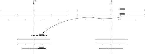
Figure 2: Illustration of the proof of Theorem 5.1. Extracting the grayed square, we have arrived at a block around sampled position $i$ in level $l$. Due to its size, the square must be contained in a half-block. This half-block (in thick line) has a copy crossing a sampled position $i^{\prime}$ (we show this copy with a dashed line). Thus the extraction task is translated to level $l+1$, inside another block of half the length. Since the square is still small enough, it must fall inside some half-block of level $l+1$ (also in thick line). This continues until the last level, where the symbols are stored directly.

5.2 Accessing $\mathit{SA}$

Let us define the differential suffix array $\mathit{DSA}[p]=\mathit{SA}[p]-\mathit{SA}[p-1]$ for all $p>1$, and $\mathit{DSA}[1]=\mathit{SA}[1]$. The next lemmas show that the runs of $\mathit{BWT}$ induce analogous repeated substrings in $\mathit{DSA}$.

Lemma 12

Let $[p-1,p]$ be within a $\mathit{BWT}$ run. Then $\mathit{LF}(p-1)=\mathit{LF}(p)-1$ and $\mathit{DSA}[\mathit{LF}(p)]=\mathit{DSA}[p]$.

Proof

Since $p$ is not the first position in a $\mathit{BWT}$ run, it holds that $\mathit{BWT}[p-1]=\mathit{BWT}[p]$, and thus $\mathit{LF}(p-1)=\mathit{LF}(p)-1$ follows from the formula of $\mathit{LF}$. Therefore, if $q=\mathit{LF}(p)$, we have $\mathit{SA}[q]=\mathit{SA}[p]-1$ and $\mathit{SA}[q-1]=\mathit{SA}[\mathit{LF}(p-1)]=\mathit{SA}[p-1]-1$; therefore $\mathit{DSA}[q]=\mathit{DSA}[p]$. ∎

Lemma 13

Let $[p-1..p+s]$ be within a $\mathit{BWT}$ run, for some $1<p\leq n$ and $0\leq s\leq n-p$. Then there exists $q\not=p$ such that $\mathit{DSA}[q..q+s]=\mathit{DSA}[p..p+s]$ and $[q-1..q+s]$ contains the first position of a $\mathit{BWT}$ run.

Proof

By Lemma 12, it holds that $\mathit{DSA}[p^{\prime}..p^{\prime}+s]=\mathit{DSA}[p..p+s]$, where $p^{\prime}=\mathit{LF}(p)$. If $\mathit{DSA}[p^{\prime}-1..p^{\prime}+s]$ contains the first position of a $\mathit{BWT}$ run, we are done. Otherwise, we apply Lemma 12 again on $[p^{\prime}..p^{\prime}+s]$, and repeat until we find a range that contains the first position of a run. This search eventually terminates because there are $r>0$ run beginnings, there are only $n-s+1$ distinct ranges, and the sequence of visited ranges, $[\mathit{LF}^{k}(p)..\mathit{LF}^{k}(p)+s]$, forms a single cycle; recall Section 2.3. Therefore our search will visit all the existing ranges before returning to $[p..p+s]$. ∎

This means that there exist $2r$ positions in $\mathit{DSA}$, namely those $[q,q+1]$ where $\mathit{BWT}[q]$ is the first position of a run, such that any substring $\mathit{DSA}[p..p+s]$ has a copy covering some of those $2r$ positions. Note that this is the same property of Lemma 8, which enabled efficient access and fingerprinting on $T$. We now exploit it to access cells in $\mathit{SA}$ by building a similar structure on $\mathit{DSA}$.

Theorem 5.2

Let the $\mathit{BWT}$ of a text $T[1..n]$ contain $r$ runs. Then there exists a data structure using $O(r\log(n/r))$ words that can retrieve any $\ell$ consecutive values of its suffix array $\mathit{SA}$ in time $O(\log(n/r)+\ell)$.

Proof

We describe a data structure supporting the extraction of $\alpha=\log(n/r)$ consecutive cells in $O(\log(n/r))$ time. To extract $\ell$ consecutive cells of $\mathit{SA}$, we divide it into $\lceil\ell/\alpha\rceil$ blocks and extract each block independently. This yields the promised time complexity.

Our structure is stored in $O(\log(n/r))$ levels. As before, let us assume that $r$ divides $n$ and that $n/r$ is a power of two. At the top level ($l=0$), we divide $\mathit{DSA}$ into $r$ blocks $\mathit{DSA}[1..n/r],\mathit{DSA}[n/r+1..2n/r],\dots,\mathit{DSA}[n-n/r+1..n]$ of size $n/r$. For levels $l>0$, we let $s_{l}=n/(r\cdot 2^{l-1})$ and, for every position $q$ that starts a run in $\mathit{BWT}$, we consider the two non-overlapping blocks of length $s_{l}$: $X_{l,q}^{1}=\mathit{DSA}[q-s_{l}+1..q]$ and $X_{l,q}^{2}=\mathit{DSA}[q+1..q+s_{l}]$. Each such block $X^{k}_{l,q}$, for $k=1,2$, is composed of two half-blocks, $X^{k}_{l,q}=X^{k}_{l,q}[1..s_{l}/2]\,X^{k}_{l,q}[s_{l}/2+1..s_{l}]$. We moreover consider three additional consecutive and non-overlapping half-blocks, starting in the middle of the first, $X^{1}_{l,q}[1..s_{l}/2]$, and ending in the middle of the last, $X^{2}_{l,q}[s_{l}/2+1..s_{l}]$, of the 4 half-blocks just described: $\mathit{DSA}[q-s_{l}+s_{l}/4+1..q-s_{l}/4],\ \mathit{DSA}[q-s_{l}/4+1..q+s_{l}/4]$, and $\mathit{DSA}[q+s_{l}/4+1..q+s_{l}-s_{l}/4]$.

From Lemma 13, blocks at level $l=0$ and each half-block at level $l>0$ have an occurrence covered by blocks at level $l+1$. Let the half-block $X$ of level $l$ (blocks at level $0$ are analogous) have an occurrence containing position $q^{*}\in\{q,q+1\}$, where $q$ starts a run in $\mathit{BWT}$. Then we store the pointer $\langle q^{*},\mathit{off},\delta\rangle$ associated with $X$, where $0<\mathit{off}\leq s_{l+1}$ indicates that the occurrence of $X$ starts at position $q^{*}-s_{l+1}+\mathit{off}$ of $\mathit{DSA}$, and $\delta=\mathit{SA}[q^{*}-s_{l+1}]-\mathit{SA}[q^{*}-s_{l+1}+\mathit{off}-1]$. (We also store the pointer to the data structure of the half-block of level $l+1$ containing the position $q^{*}$.)

Additionally, every level-0 block $X^{\prime}=\mathit{DSA}[q^{\prime}+1..q^{\prime}+s_{l}]$ stores the value $S(X^{\prime})=\mathit{SA}[q^{\prime}]$ (assume $\mathit{SA}[0]=0$ throughout), and every half-block $X^{\prime}=\mathit{DSA}[q^{\prime}+1..q^{\prime}+s_{l+1}/2]$ corresponding to the area $X_{l+1,q}^{1}X_{l+1,q}^{2}=\mathit{DSA}[q-s_{l+1}+1..q+s_{l+1}]$ stores the value $\Delta(X^{\prime})=\mathit{SA}[q^{\prime}]-\mathit{SA}[q-s_{l+1}]$.

Let $l^{*}$ be the smallest number such that $s_{l^{*}}<4\alpha=4\log(n/r)$. Then $l^{*}$ is the last level of our structure. At this level, we explicitly store the sequence of $\mathit{DSA}$ cells of the areas $X_{l^{*},q}^{1}X_{l^{*},q}^{2}$, for each $q$ starting a run in $\mathit{BWT}$. This uses in total $O(r\cdot s_{l^{*}})=O(r\log(n/r))$ words of space. The pointers stored for the $O(r)$ blocks at previous levels also add up to $O(r\log(n/r))$ words.

Let $S=\mathit{SA}[p..p+\alpha-1]$ be the sequence of cells to be extracted. This range either spans two blocks at level 0, or it is contained in a single block. In the former case, we decompose it into two queries that are fully contained inside a block at level $0$. To retrieve a range contained in a single block or half-block, we map it down to the next levels using the pointers from blocks and half-blocks, as a contiguous sequence as long as it fits inside a single half-block. This is always possible as long as $\alpha\leq s_{l}/4$. By definition, then, we arrive in this way precisely to level $l^{*}$, where the symbols of $\mathit{DSA}$ are stored explicitly and we can return the sequence.

We need, however, the contents of $\mathit{SA}[p..p+\alpha-1]$, not of $\mathit{DSA}[p..p+\alpha-1]$. To obtain the former from the latter, we need only the value of $\mathit{SA}[p]$. During the traversal, we will maintain a value $f$ with the invariant that, whenever the original position $\mathit{DSA}[p]$ has been mapped to a position $X[p^{\prime}]$ in the current block $X$, then it holds that $\mathit{SA}[p]=f+X[1]+\ldots+X[p^{\prime}]$. This invariant must be maintained when we use pointers, where the original $\mathit{DSA}$ values in a block $X$ are obtained from a copy that appears somewhere else in $\mathit{DSA}$.

The invariant is initially valid by setting $f$ to the $S(X)$ value associated with the level-0 block $X$ that contains $\mathit{SA}[p]$. When we follow a pointer $\langle q,\mathit{offs},\delta\rangle$ and choose $X^{\prime}$ from the 7 half-blocks that cover the target, we update $f\leftarrow f+\delta+\Delta(X^{\prime})$. When we arrive at a block $X$ at level $l^{*}$, we scan $O(\alpha)$ symbols until reaching the first value of the desired position $X[p^{\prime}]$. The values $X[1],\ldots,X[p^{\prime}]$ scanned are also summed to $f$. At the end, we have that $\mathit{SA}[p]=f$. See Figure 3. ∎

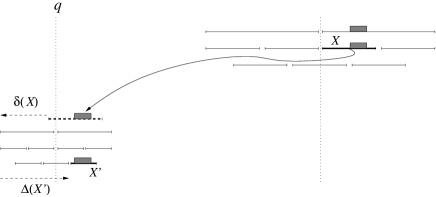
Figure 3: Illustration of Theorem 5.2. The area to extract (a gray square) is inside the thick half-block ($X$), which points inside another area around position $q$ in the next level. The sum of $\mathit{DSA}$ over the offset from the beginning of the area to the mapped block (in thick dashed line) is stored at $\delta(X)$, in negative (hence the direction of the arrow). The squared area is mapped to a smaller half-block, $X^{\prime}$, which records in $\Delta(X^{\prime})$ the sum of $\mathit{DSA}$ between the beginning of the area and $X^{\prime}$ (see the other dashed arrow). By adding $\delta(X)+\Delta(X^{\prime})$, we map from the first thick block to the second.

5.3 Accessing $\mathit{ISA}$ and $\mathit{LCP}$

A similar method can be used to access inverse suffix array cells, $\mathit{ISA}[i]$. Let us define $\mathit{DISA}[i]=\mathit{ISA}[i]-\mathit{ISA}[i-1]$ for all $i>1$, and $\mathit{DISA}[1]=\mathit{ISA}[1]$. The role of the runs in $\mathit{SA}$ will now be played by the phrases in $\mathit{ISA}$, which will be defined analogously as in the proof of Lemma 3: Phrases in $\mathit{ISA}$ start at the positions $\mathit{SA}[p]$ such that a new run starts in $\mathit{BWT}[p]$ (here, last positions of runs do not start phrases). Instead of $\mathit{LF}$, we use the cycle $\phi(i)$ of Definition 2. We make use of the following lemmas.

Lemma 14

Let $[i-1..i]$ be within a phrase of $\mathit{ISA}$. Then it holds that $\phi(i-1)=\phi(i)-1$ and $\mathit{DISA}[i]=\mathit{DISA}[\phi(i)]$.

Proof

Consider the pair of positions $T[i-1..i]$ within a phrase. Let them be pointed from $\mathit{SA}[p]=i$ and $\mathit{SA}[q]=i-1$, therefore $\mathit{ISA}[i]=p$, $\mathit{ISA}[i-1]=q$, and $\mathit{LF}(p)=q$. Now, since $i$ is not a phrase beginning, $p$ is not the first position in a $\mathit{BWT}$ run. Therefore, $\mathit{BWT}[p-1]=\mathit{BWT}[p]$, from which it follows that $\mathit{LF}(p-1)=\mathit{LF}(p)-1=q-1$. Now let $\mathit{SA}[p-1]=j$, that is, $j=\phi(i)$. Then $\phi(i-1)=\mathit{SA}[\mathit{ISA}[i-1]-1]=\mathit{SA}[q-1]=\mathit{SA}[\mathit{LF}(p-1)]=\mathit{SA}[p-1]-1=j-1=\phi(i)-1$. It also follows that $\mathit{DISA}[i]=p-q=\mathit{DISA}[j]=\mathit{DISA}[\phi(i)]$. ∎

Lemma 15

Let $[i-1..i+s]$ be within a phrase of $\mathit{DISA}$, for some $1<i\leq n$ and $0\leq s\leq n-i$. Then there exists $j\not=i$ such that $\mathit{DISA}[j..j+s]=\mathit{DISA}[i..i+s]$ and $[j-1..j+s]$ contains the first position of a phrase.

Proof

By Lemma 14, it holds that $\mathit{DISA}[i^{\prime}..i^{\prime}+s]=\mathit{DISA}[i..i+s]$, where $i^{\prime}=\phi(i)$. If $\mathit{DISA}[i^{\prime}-1..i^{\prime}+s]$ contains the first position of a phrase, we are done. Otherwise, we apply Lemma 14 again on $[i^{\prime}..i^{\prime}+s]$, and repeat until we find a range that contains the first position of a phrase. Just as in Lemma 12, this search eventually terminates because $\phi$ is a permutation with a single cycle. ∎

We can then use on $\mathit{DISA}$ exactly the same data structure we defined to access $\mathit{SA}$ in Theorem 5.2, and obtain a similar result for $\mathit{ISA}$.

Theorem 5.3

Let the $\mathit{BWT}$ of a text $T[1..n]$ contain $r$ runs. Then there exists a data structure using $O(r\log(n/r))$ words that can retrieve any $\ell$ consecutive values of its inverse suffix array $\mathit{ISA}$ in time $O(\log(n/r)+\ell)$.

Finally, by combining Theorem 5.2 and Lemma 5, we also obtain access to array $\mathit{LCP}$ without knowing the corresponding text positions.

Theorem 5.4

Let the $\mathit{BWT}$ of a text $T[1..n]$ contain $r$ runs. Then there exists a data structure using $O(r\log(n/r))$ words that can retrieve any $\ell$ consecutive values of its longest common prefix array $\mathit{LCP}$ in time $O(\log(n/r)+\ell)$.

Proof

Build the structure of Theorem 5.2, as well as the one of Lemma 5 with $s=\log(n/r)$. Then, to retrieve $\mathit{LCP}[p..p+s^{\prime}-1]$ for any $0\leq s^{\prime}\leq s$, we first compute $\mathit{SA}[p]$ in time $O(\log(n/r))$ using Theorem 5.2 and then, given $\mathit{SA}[p]$, we compute $\mathit{LCP}[p..p+s^{\prime}-1]$ using Lemma 5 in time $O(\log\log_{w}(n/r)+s^{\prime})$. Adding both times gives $O(\log(n/r))$.

To retrieve an arbitrary sequence of cells $\mathit{LCP}[p..p+\ell-1]$, we use the method above by chunks of $s$ cells, plus a possibly smaller final chunk. As we use $\lceil\ell/s\rceil$ chunks, the total time is $O(\log(n/r)+\ell)$. ∎

5.4 Optimal counting and locating in $O(r\log(n/r))$ space

The $O(r\log(n/r))$ space we need for accessing $T$ is not comparable with the $O(r\log\log_{w}(\sigma+n/r))$ space we need for optimal counting and locating. The latter is in general more attractive, because the former is better whenever $r=\omega(n/\log_{w}\sigma)$, which means that the text is not very compressible. Anyway, we show how to obtain optimal counting and locating within space $O(r\log(n/r))$.

By the discussion above, we only have to care about the case $r\geq n/\log n$. In such a case, it holds that $r\log(n/r)\geq(n\log\log n)/\log n$, and thus we are allowed to use $\Theta(n\log\log n)$ bits of space. We can then make use of a result of Belazzougui and Navarro [12, Lem. 6]. They show how we can enrich the $O(n)$-bit compressed suffix tree of Sadakane [106] so that, using $O(n(\log t_{\mathit{SA}}+\log\log\sigma))$ bits, one can find the interval $\mathit{SA}[sp..ep]$ of $P$ in time $O(m+t_{\mathit{SA}})$ plus the time to extract a substring of length $m$ from $T$. Since we provide $t_{\mathit{SA}}=O(\log(n/r))$ in Theorem 5.2 and extraction time $O(\log(n/r)+m\log(\sigma)/w)$ in Theorem 5.1, this arrangement uses $O(n(\log\log(n/r)+\log\log\sigma))\subseteq O(n\log\log n)$ bits, and it supports counting in time $O(m+\log(n/r))$.

Once we know the interval, apart from counting, we can use Theorem 5.2 to obtain $\mathit{SA}[p]$ for any $sp\leq p\leq ep$ in time $O(\log(n/r))$, and then use the structure of Lemma 4 with $s=\log(n/r)$ to extract packs of $s^{\prime}\leq s$ consecutive $\mathit{SA}$ entries in time $O(\log\log_{w}(n/r)+s^{\prime})\subseteq O(\log(n/r)+s)$. Overall, we can locate the $occ$ occurrences of $P$ in time $O(m+\log(n/r)+occ)$.

Finally, to remove the $O(\log(n/r))$ term in the times, we must speed up the searches for patterns shorter than $\log(n/r)$. We index them using a compact trie as that of Section 4.2. We store in each explicit trie node (i) the number of occurrences of the corresponding string, to support counting, and (ii) a position $p$ where it occurs in $\mathit{SA}$, the value $\mathit{SA}[p]$, and the result of the predecessor queries on $P^{+}$ and $P^{-}$, as required for locating in Lemma 4, so that we can retrieve any number $s^{\prime}\leq s$ of consecutive entries of $\mathit{SA}$ in time $O(s^{\prime})$. By Lemma 9, the size of the trie and of the text substrings explicitly stored to support path compression is $O(r\log(n/r))$.

Theorem 5.5

We can store a text $T[1..n]$, over alphabet $[1..\sigma]$, in $O(r\log(n/r))$ words, where $r$ is the number of runs in the BWT of $T$, such that later, given a pattern $P[1..m]$, we can count the occurrences of $P$ in $T$ in $O(m)$ time and (after counting) report their $occ$ locations in overall time $O(occ)$.

6 A Run-Length Compressed Suffix Tree

In this section we show how to implement a compressed suffix tree within $O(r\log(n/r))$ words, which solves a large set of navigation operations in time $O(\log(n/r))$. The only exceptions are going to a child by some letter and performing level ancestor queries, which may cost as much as $O(\log(n/r)\log n)$. The first compressed suffix tree for repetitive collections was built on runs [80], but just like the self-index, it needed $\Theta(n/s)$ space to obtain $O(s\log n)$ time in key operations like accessing $\mathit{SA}$. Other compressed suffix trees for repetitive collections appeared later [1, 92, 29], but they do not offer formal space guarantees (see later). A recent one, instead, uses $O(\overline{e})$ words and supports a number of operations in time typically $O(\log n)$ [8]. The two space measures are not comparable.

6.1 Compressed Suffix Trees without Storing the Tree

Fischer et al. [37] showed that a rather complete suffix tree functionality including all the operations in Table 3 can be efficiently supported by a representation where suffix tree nodes $v$ are identified with the suffix array intervals $\mathit{SA}[v_{l}..v_{r}]$ they cover. Their representation builds on the following primitives:

1. Access to arrays $\mathit{SA}$ and $\mathit{ISA}$, in time we call $t_{\mathit{SA}}$.

2. Access to array $\mathit{LCP}$, in time we call $t_{\mathit{LCP}}$.

3. Three special queries on $\mathit{LCP}$:

   1. Range Minimum Query,

      $$\mathrm{RMQ}(i,j)=\arg\min_{i\leq k\leq j}\mathit{LCP}[k],$$

      choosing the leftmost one upon ties, in time we call $t_{\mathrm{RMQ}}$.

   2. Previous/Next Smaller Value queries,

      $$\mathrm{PSV}(p) = \max(\{q<p,\mathit{LCP}[q]<\mathit{LCP}[p]\}\cup\{0\}),$$

      $$\mathrm{NSV}(p) = \min(\{q>p,\mathit{LCP}[q]<\mathit{LCP}[p]\}\cup\{n+1\}),$$

      in time we call $t_{\mathrm{SV}}$.

Operation	Description
Root()	Suffix tree root.
Locate($v$)	Text position $i$ of leaf $v$.
Ancestor($v,w$)	Whether $v$ is an ancestor of $w$.
SDepth($v$)	String depth for internal nodes, i.e., length of string represented by $v$.
TDepth($v$)	Tree depth, i.e., depth of tree node $v$.
Count($v$)	Number of leaves in the subtree of $v$.
Parent($v$)	Parent of $v$.
FChild($v$)	First child of $v$.
NSibling($v$)	Next sibling of $v$.
SLink($v$)	Suffix-link, i.e., if $v$ represents $a\cdot\alpha$ then the node that represents $\alpha$, for $a\in[1..\sigma]$.
WLink($v,a$)	Weiner-link, i.e., if $v$ represents $\alpha$ then the node that represents $a\cdot\alpha$.
SLinki($v$)	Iterated suffix-link.
LCA($v,w$)	Lowest common ancestor of $v$ and $w$.
Child($v,a$)	Child of $v$ by letter $a$.
Letter($v,i$)	The $ith$ letter of the string represented by $v$.
LAQS($v,d$)	String level ancestor, i.e., the highest ancestor of $v$ with string-depth $\geq d$.
LAQT($v,d$)	Tree level ancestor, i.e., the ancestor of $v$ with tree-depth $d$.

Table 3: Suffix tree operations.

An interesting finding of Fischer et al. [37] related to our results is that array $\mathit{PLCP}$, which stores the $\mathit{LCP}$ values in text order, can be stored in $O(r)$ words and accessed efficiently; therefore we can compute any $\mathit{LCP}$ value in time $t_{\mathit{SA}}$ (see also Fischer [34]). We obtained a generalization of this property in Section 3.2. They [37] also show how to represent the array $\mathit{TDE}[1..n]$, where $\mathit{TDE}[i]$ is the tree-depth of the lowest common ancestor of the $(i-1)$th and $i$th suffix tree leaves (and $\mathit{TDE}[1]=0$). Fischer et al. [37] represent its values in text order in an array $\mathit{PTDE}$, which just like $\mathit{PLCP}$ can be stored in $O(r)$ words and accessed efficiently, thereby giving access to $\mathit{TDE}$ in time $t_{\mathit{SA}}$. They use $\mathit{TDE}$ to compute operations TDepth and LAQ_T efficiently.

Abeliuk et al. [1] show that primitives $\mathrm{RMQ}$, $\mathrm{PSV}$, and $\mathrm{NSV}$ can be implemented using a simplified variant of range min-Max trees (rmM-trees) [95], consisting of a perfect binary tree on top of $\mathit{LCP}$ where each node stores the minimum $\mathit{LCP}$ value in its subtree. The three primitives are then computed in logarithmic time. They define the extended primitives

$$\mathrm{PSV}^{\prime}(p,d) = \max(\{q<p,\mathit{LCP}[q]<d\}\cup\{0\}),$$

$$\mathrm{NSV}^{\prime}(p,d) = \min(\{q>p,\mathit{LCP}[q]<d\}\cup\{n+1\}),$$

and compute them in time $t_{\mathrm{SV}^{\prime}}$, which in their setting is the same $t_{\mathrm{SV}}$ of the basic $\mathrm{PSV}$ and $\mathrm{NSV}$ primitives. The extended primitives are used to simplify some of the operations of Fischer et al. [37].

The resulting time complexities are given in the second column of Table 4, where $t_{\mathit{LF}}$ is the time to compute function $\mathit{LF}$ or its inverse, or to access a position in $\mathit{BWT}$. Operation WLink, not present in Fischer et al. [37], is trivially obtained with two $\mathit{LF}$-steps. We note that most times appear multiplied by $t_{\mathit{LCP}}$ in Fischer et al. [37] because their $\mathrm{RMQ}$, $\mathrm{PSV}$, and $\mathrm{NSV}$ structures do not store $\mathit{LCP}$ values inside, so they need to access the array all the time; this is not the case when we use rmM-trees. The time of LAQ_S is due to improvements obtained with the extended primitives $\mathrm{PSV}^{\prime}$ and $\mathrm{NSV}^{\prime}$ [1]. The time for Child($v,a$) is obtained by binary searching among the $\sigma$ minima of $\mathit{LCP}[v_{l},v_{r}]$, and extracting the desired letter (at position SDepth$(v)+1$) to compare with $a$. Each binary search operation can be done with an extended primitive $\mathrm{RMQ}^{\prime}(p,q,m)$ that finds the $m$th left-to-right occurrence of the minimum in a range. This is easily done in $t_{\mathrm{RMQ}^{\prime}}=t_{\mathrm{RMQ}}$ time on a rmM-tree by storing, in addition, the number of times the minimum of each node occurs below it [95], but it may be not so easy to do on other structures. Finally, the complexities of TDepth and LAQ_T make use of array $\mathit{TDE}$. While Fischer et al. [37] use an $\mathrm{RMQ}$ operation to compute TDepth, we note that TDepth$(v)=1+\max(\mathit{TDE}[v_{l}],\mathit{TDE}[v_{r}+1])$, because the suffix tree has no unary nodes (they used this simpler formula only for leaves).

Operation	Generic	Our
	Complexity	Complexity
Root()	$1$	$1$
Locate($v$)	$t_{\mathit{SA}}$	$\log(n/r)$
Ancestor($v,w$)	$1$	$1$
SDepth($v$)	$t_{\mathrm{RMQ}}+t_{\mathit{LCP}}$	$\log(n/r)$
TDepth($v$)	$t_{\mathit{SA}}$	$\log(n/r)$
Count($v$)	$1$	$1$
Parent($v$)	$t_{\mathit{LCP}}+t_{\mathrm{SV}}$	$\log(n/r)$
FChild($v$)	$t_{\mathrm{RMQ}}$	$\log(n/r)$
NSibling($v$)	$t_{\mathit{LCP}}+t_{\mathrm{RMQ}}$	$\log(n/r)$
SLink($v$)	$t_{\mathit{LF}}+t_{\mathrm{RMQ}}+t_{\mathrm{SV}}$	$\log(n/r)$
WLink($v$)	$t_{\mathit{LF}}$	$\log\log_{w}(n/r)$
SLinki($v$)	$t_{\mathit{SA}}+t_{\mathrm{RMQ}}+t_{\mathrm{SV}}$	$\log(n/r)$
LCA($v,w$)	$t_{\mathrm{RMQ}}+t_{\mathrm{SV}}$	$\log(n/r)$
Child($v,a$)	$t_{\mathit{LCP}}+(t_{\mathrm{RMQ}^{\prime}}+t_{\mathit{SA}}+t_{\mathit{LF}})\log\sigma$	$~{}~{}~{}~{}\log(n/r)\log\sigma~{}~{}~{}~{}$
Letter($v,i$)	$t_{\mathit{SA}}+t_{\mathit{LF}}$	$\log(n/r)$
LAQS($v,d$)	$t_{\mathrm{SV}^{\prime}}$	$\log(n/r)+\log\log_{w}r$
LAQT($v,d$)	$(t_{\mathrm{RMQ}}+t_{\mathit{LCP}})\log n$	$\log(n/r)\log n$

Table 4: Complexities of suffix tree operations. Letter($v,i$) can also be solved in time $O(i\cdot t_{\mathit{LF}})=O(i\log\log_{w}(n/r))$.

An important idea of Abeliuk et al. [1] is that they represent $\mathit{LCP}$ differentially, that is, the array $\mathit{DLCP}[1..n]$, where $\mathit{DLCP}[i]=\mathit{LCP}[i]-LCP[i-1]$ if $i>1$ and $\mathit{DLCP}[1]=\mathit{LCP}[1]$, using a context-free grammar (CFG). Further, they store the rmM-tree information in the nonterminals, that is, a nonterminal $X$ expanding to a substring $D$ of $\mathit{DLCP}$ stores the (relative) minimum

$$m(X)~{}=~{}\min_{0\leq k\leq|D|}\sum_{i=1}^{k}D[i]$$

of any $\mathit{LCP}$ segment having those differential values, and its position inside the segment,

$$p(X)~{}=~{}\arg\min_{0\leq k\leq|D|}\sum_{i=1}^{k}D[i].$$

Thus, instead of a perfect rmM-tree, they conceptually use the grammar tree as an rmM-tree. They show how to adapt the algorithms on the perfect rmM-tree to run on the grammar, and thus solve primitives $\mathrm{RMQ}$, $\mathrm{PSV}^{\prime}$, and $\mathrm{NSV}^{\prime}$, in time proportional to the grammar height.

Abeliuk et al. [1], and also Fischer et al. [37], claim that the grammar produced by RePair [75] is of size $O(r\log(n/r))$. This is an incorrect result borrowed from González et al. [51, 52], where it was claimed for $\mathit{DSA}$. The proof fails for a reason we describe in our technical report [44, Sec. A].

We now start by showing how to build a grammar of size $O(r\log(n/r))$ and height $O(\log(n/r))$ for $\mathit{DLCP}$. This grammar is of an extended type called run-length context-free grammar (RLCFG) [97], which allows rules of the form $X\rightarrow Y^{t}$ that count as size 1. We then show how to implement the operations $\mathrm{RMQ}$ and $\mathrm{NSV}/\mathrm{PSV}$ in time $O(\log(n/r))$ on the resulting RLCFG, and $\mathrm{NSV}^{\prime}/\mathrm{PSV}^{\prime}$ in time $O(\log(n/r)+\log\log_{w}r)$. Finally, although we cannot implement $\mathrm{RMQ}^{\prime}$ in time below $\Theta(\log n)$, we show how the specific Child operation can be implemented in time $O(\log(n/r)\log\sigma)$.

Note that, although we could represent $\mathit{DLCP}$ using a Block-Tree-like structure as we did in Section 5 for $\mathit{DSA}$ and $\mathit{DISA}$, we have not devised a way to implement the more complex operations we need on $\mathit{DLCP}$ using such a Block-Tree-like data structure within polylogarithmic time.

Using the results we obtain in this and previous sections, that is, $t_{\mathit{SA}}=O(\log(n/r))$, $t_{\mathit{LF}}=O(\log\log_{w}(n/r))$, $t_{\mathit{LCP}}=t_{\mathit{SA}}+O(\log\log_{w}(n/r))=O(\log(n/r))$, $t_{\mathrm{RMQ}}=t_{\mathrm{SV}}=O(\log(n/r))$, $t_{SV^{\prime}}=O(\log(n/r)+\log\log_{w}r)$, and our specialized algorithm for Child, we obtain our result.

Theorem 6.1

Let the $\mathit{BWT}$ of a text $T[1..n]$, over alphabet $[1..\sigma]$, contain $r$ runs. Then a compressed suffix tree on $T$ can be represented using $O(r\log(n/r))$ words, and it supports the operations with the complexities given in the third column of Table 4.

6.2 Representing $\mathit{DLCP}$ with a run-length grammar

In this section we show that the differential array $\mathit{DLCP}$ can be represented by a RLCFG of size $O(r\log(n/r))$. We first prove a lemma analogous to those of Section 5.

Lemma 16

Let $[p-2,p]$ be within a $\mathit{BWT}$ run. Then $\mathit{LF}(p-1)=\mathit{LF}(p)-1$ and $\mathit{DLCP}[\mathit{LF}(p)]=\mathit{DLCP}[p]$.

Proof

Let $i=\mathit{SA}[p]$, $j=\mathit{SA}[p-1]$, and $k=\mathit{SA}[p-2]$. Then $\mathit{LCP}[p]=lcp(T[i..],T[j..])$ and $\mathit{LCP}[p-1]=lcp(T[j..],T[k..])$. We know from Lemma 12 that, if $q=\mathit{LF}(p)$, then $\mathit{LF}(p-1)=q-1$ and $\mathit{LF}(p-2)=q-2$. Also, $\mathit{SA}[q]=i-1$, $\mathit{SA}[q-1]=j-1$, and $\mathit{SA}[q-2]=k-1$. Therefore, $\mathit{LCP}[\mathit{LF}(p)]=\mathit{LCP}[q]=lcp(T[\mathit{SA}[q]..],T[\mathit{SA}[q-1]..)=lcp(T[i-1..],T[j-1..])$. Since $p$ is not the first position in a $\mathit{BWT}$ run, it holds that $T[j-1]=\mathit{BWT}[p-1]=\mathit{BWT}[p]=T[i-1]$, and thus $lcp(T[i-1..],T[j-1..])=1+lcp(T[i..],T[j..])=1+\mathit{LCP}[p]$. Similarly, $\mathit{LCP}[\mathit{LF}(p)-1]=\mathit{LCP}[q-1]=lcp(T[\mathit{SA}[q-1]..],T[\mathit{SA}[q-2]..)=lcp(T[j-1..],T[k-1..])$. Since $p-1$ is not the first position in a $\mathit{BWT}$ run, it holds that $T[k-1]=\mathit{BWT}[p-2]=\mathit{BWT}[p-1]=T[j-1]$, and thus $lcp(T[j-1..],T[k-1..])=1+lcp(T[j..],T[k..])=1+\mathit{LCP}[p-1]$. Therefore $\mathit{DLCP}[q]=\mathit{LCP}[q]-\mathit{LCP}[q-1]=(1+\mathit{LCP}[p])-(1+\mathit{LCP}[p-1])=\mathit{DLCP}[p]$. ∎

It follows that, if $p_{1}<\ldots<p_{r}$ are the positions that start runs in $\mathit{BWT}$, then we can define a bidirectional macro scheme [110] of size at most $4r+1$ on $\mathit{DLCP}$.

Definition 6

A bidirectional macro scheme (BMS) of size $b$ on a sequence $S[1..n]$ is a partition $S=S_{1}\ldots S_{b}$ such that each $S_{k}$ is of length 1 (and is represented as an explicit symbol) or it appears somewhere else in $S$ (and is represented by a pointer to that other occurrence). Let $f(i)$, for $1\leq i\leq n$, be defined arbitrarily if $S[i]$ is an explicit symbol, and $f(i)=j+i^{\prime}-1$ if $S[i]=S_{k}[i^{\prime}]$ is inside some $S_{k}$ that is represented as a pointer to $S[j..j^{\prime}]$. A correct BMS must hold that, for any $i$, there is a $k\geq 0$ such that $f^{k}(i)$ is an explicit symbol.

Note that $f(i)$ maps the position $S[i]$ to the source from which it is to be obtained. The last condition then ensures that we can recover any symbol $S[i]$ by following the chain of copies until finding an explicitly stored symbol. Finally, note that all the $f$ values inside a block are consecutive: if $S_{k}=S[i..i^{\prime}]$ has a pointer to $S[j..j^{\prime}]$, then $f([i..i^{\prime}])=[j..j^{\prime}]$.

Lemma 17

Let $p_{1}<\ldots<p_{r}$ be the positions that start runs in $\mathit{BWT}$, and assume $p_{0}=-2$ and $p_{r+1}=n+1$. Then, the partition formed by (1) all the explicit symbols $\mathit{DLCP}[p_{i}+k]$ for $1\leq i\leq r$ and $k\in\{0,1,2\}$, and (2) all the nonempty regions $\mathit{DLCP}[p_{i}+3..p_{i+1}-1]$ for all $0\leq i\leq r$, pointing to $\mathit{DLCP}[\mathit{LF}(p_{i}+3)..\mathit{LF}(p_{i+1}-1)]$, is a BMS.

Proof

By Lemma 16, it holds that $\mathit{LF}(p_{i}+3+k)=\mathit{LF}(p_{i}+3)+k$ and $\mathit{DLCP}[p_{i}+3+k]=\mathit{DLCP}[\mathit{LF}(p_{i}+3)+k]$ for all $0\leq k\leq p_{i+1}-p_{i}-4$, so the partition is well defined and the copies are correct. To see that it is a BMS, it is sufficient to notice that $\mathit{LF}$ is a permutation with one cycle on $[1..n]$, and therefore $\mathit{LF}^{k}(p)$ will eventually reach an explicit symbol, for some $0\leq k<n$. ∎

We now make use of the following result.

Lemma 18 ([45, Thm. 1])

Let $S[1..n]$ have a BMS of size $b$. Then there exists a RLCFG of size $O(b\log(n/b))$ that generates $S$.

Since $\mathit{DLCP}$ has a BMS of size at most $4r+1$, the following corollary is immediate.

Lemma 19

Let the $\mathit{BWT}$ of $T[1..n]$ have $r$ runs. Then there exists a RLCFG of size $O(r\log(n/r))$ that generates its differential $\mathit{LCP}$ array, $\mathit{DLCP}$.

6.3 Supporting the primitives on the run-length grammar

We describe how to compute the primitives $\mathrm{RMQ}$ and $\mathrm{PSV}/\mathrm{NSV}$ on the RLCFG of $\mathit{DLCP}$, in time $t_{\mathrm{RMQ}}=t_{\mathrm{SV}}=O(\log(n/r))$. The extended primitives $\mathrm{PSV}^{\prime}/\mathrm{NSV}^{\prime}$ are solved in time $t_{SV^{\prime}}=O(\log(n/r)+\log\log_{w}r)$. While analogous procedures have been described before on CFGs and trees [1, 95], the extension to RLCFGs and the particular structure of our grammar requires a complete description.

The RLCFG built in Lemma 18 [45] is of height $O(\log(n/r))$ and has one initial rule $S\rightarrow X_{1}\ldots X_{O(r)}$. The other rules are of the form $X\rightarrow Y_{1}Y_{2}$ or $X\rightarrow Y^{t}$ for $t>2$. All the right-hand symbols can be terminals or nonterminals.

The data structure we use is formed by a sequence $\mathit{DLCP}^{\prime}=X_{1}\ldots X_{O(r)}$ capturing the initial rule of the RLCFG, and an array of the other $O(r\log(n/r))$ rules. For each nonterminal $X$ expanding to a substring $D$ of $\mathit{DLCP}$, we store its length $l(X)=|D|$ and its total difference $d(X)=D[1]+\ldots+D[l(X)]$. For terminals $X$, assume $l(X)=1$ and $d(X)=X$. We also store a cumulative length array $L[0]=0$ and $L[x]=L[x-1]+l(X_{x})$ that can be binary searched to find the symbol of $\mathit{DLCP}^{\prime}$ that contains any desired position $\mathit{DLCP}[p]$. To ensure that this binary search takes time $O(\log(n/r))$ when $r=\omega(n/r)$, we can store a sampled array of positions $S[1..r]$, where $S[t]=x$ if $L[x-1]<t\cdot(n/r)\leq L[x]$ to narrow down the binary search to a range of $O(n/r)$ entries of $L$. We also store a cumulative differences array $A[0]=0$ and $A[x]=A[x-1]+d(X_{x})$.

Although we have already provided access to any $\mathit{LCP}[p]$ in Section 5.3, it is also possible to do it with these structures. We first find $x$ by binary searching $L$ for $p$, possibly with the help of $S$, and set $f\leftarrow A[x-1]$ and $p\leftarrow p-L[x-1]$. Then we enter recursively into nonterminal $X=X_{x}$. If its rule is $X\rightarrow Y_{1}Y_{2}$, we continue by $Y_{1}$ if $p\leq l(Y_{1})$; otherwise we set $f\leftarrow f+d(Y_{1})$, $p\leftarrow p-l(Y_{1})$, and continue by $Y_{2}$. If, instead, its rule is $X\rightarrow Y^{t}$, we compute $t^{\prime}=\lceil p/l(Y)\rceil-1$, set $f\leftarrow f+t^{\prime}\cdot d(Y)$, $p\leftarrow p-t^{\prime}\cdot l(Y)$, and continue by $Y$. When we finally arrive at a terminal $X$, the answer is $f+d(X)$. All this process takes time $O(\log(n/r))$, the height of the RLCFG.

Answering $\mathrm{RMQ}$.

To answer this query, we store a few additional structures. We store an array $M$ such that $M[x]=\min_{L[x-1]<k\leq L[x]}\mathit{LCP}[k]$, that is, the minimum value in the area of $\mathit{LCP}$ expanded by $X_{x}=\mathit{DLCP}^{\prime}[x]$. We store a succinct data structure $\mathrm{RMQ}_{M}$, which requires just $O(r)$ bits and finds the leftmost position of a minimum in any range $M[x..y]$ in constant time, without need to access $M$ [36]. We also store, for each nonterminal $X$, the already defined values $m(X)$ and $p(X)$ (for terminals $X$, we can store $m(X)$ and $p(X)$ or compute them on the fly).

To compute $\mathrm{RMQ}(p,q)$ on $\mathit{LCP}$, we first use $L$ and $S$ to determine that $\mathit{DLCP}[p..q]$ contains the expansion of $\mathit{DLCP}^{\prime}[x+1..y-1]$, whereas $\mathit{DLCP}^{\prime}[x..y]$ expands to $\mathit{DLCP}[p^{\prime}..q^{\prime}]$ with $p^{\prime}<p\leq q<q^{\prime}$. Thus, $\mathit{DLCP}[p..q]$ partially overlaps $\mathit{DLCP}^{\prime}[x]$ and $\mathit{DLCP}^{\prime}[y]$ (the overlap could be empty). We first obtain in constant time the minimum position of the central area, $z=\mathrm{RMQ}_{M}(x+1,y-1)$, and then the minimum value in that area is $\mathit{LCP}[L[z-1]+p(X_{z})]$. To complete the query, we must compare this value with the minima in $X_{x}\langle p-p^{\prime}+1,l(X_{x})\rangle$ and $X_{y}\langle 1,l(X_{y})+q-q^{\prime}\rangle$, where $X\langle a,b\rangle$ refers to the substring $D[a..b]$ in the expansion $D$ of $X$. A relevant special case in this scheme is that $\mathit{DLCP}[p..q]$ is inside a single symbol $\mathit{DLCP}^{\prime}[x]$ expanding to $\mathit{DLCP}[p^{\prime}..q^{\prime}]$, in which case the query boils down to finding the minimum value in $X_{x}\langle p-p^{\prime}+1,l(X_{x})+q-q^{\prime}\rangle$.

Let us disregard the rules $X\rightarrow Y^{t}$ for a moment. To find the minimum in $X_{w}\langle a,b\rangle$, we identify the $k=O(\log(n/r))$ maximal nodes of the grammar tree that cover the range $[a..b]$ in the expansion of $X_{w}$. Let these nodes be $Y_{1},Y_{2},\ldots,Y_{k}$. We then find the minimum of $m(Y_{1})$, $d(Y_{1})+m(Y_{2})$, $d(Y_{1})+d(Y_{2})+m(Y_{3})$, $\ldots$, in $O(k)$ time. Once the minimum is identified at $Y_{s}$, we obtain the absolute value by extracting $\mathit{LCP}[L[w-1]+l(Y_{1})+\ldots+l(Y_{s-1})+p(Y_{s})]$.

Our grammar also has rules of the form $X\rightarrow Y^{t}$, and thus the maximal coverage $Y_{1},\ldots,Y_{k}$ may include a part of these rules, say $Y^{t^{\prime}}$ for some $1\leq t^{\prime}<t$. We can then compute on the fly $m(Y^{t^{\prime}})$ as $m(Y)$ if $d(Y)\geq 0$, and $(t^{\prime}-1)\cdot d(Y)+m(Y)$ otherwise. Similarly, $p(Y^{t^{\prime}})$ is $p(Y)$ if $d(Y)\geq 0$ and $(t^{\prime}-1)\cdot l(Y)+p(Y)$ otherwise.

Once we have the (up to) three minima from $X_{x}$, $\mathit{DLCP}^{\prime}[x+1..y-1]$, and $X_{y}$, the position of the smallest of the three is $\mathrm{RMQ}(p,q)$.

Answering $\mathrm{PSV}/\mathrm{NSV}$ and $\mathrm{PSV}^{\prime}/\mathrm{NSV}^{\prime}$.

These queries are solved analogously. Let us describe $\mathrm{NSV}^{\prime}(p,d)$, since $\mathrm{PSV}^{\prime}(p,d)$ is similar. Let $\mathit{DLCP}[p..]$ be included in the expansion of $\mathit{DLCP}^{\prime}[x..]$, which expands to $\mathit{DLCP}[p^{\prime}..]$ (for the largest possible $p^{\prime}\leq p$), and let us subtract $\mathit{LCP}[p^{\prime}-1]=A[x-1]$ from $d$ to put it in relative form. We first consider $X_{x}\langle p-p^{\prime}+1,l(X_{x})\rangle=X\langle a,b\rangle$, obtaining the $O(\log(n/r))$ maximal nonterminals $Y_{1},Y_{2},\ldots,Y_{k}$ that cover $X\langle a,b\rangle$, and find the first $Y_{s}$ where $d(Y_{1})+\ldots+d(Y_{s-1})+m(Y_{s})<d$. Then we subtract $d(Y_{1})+\ldots+d(Y_{s-1})$ from $d$, add $l(Y_{1})+\ldots+l(Y_{s-1})$ to $p$, and continue recursively inside $Y_{s}$ to find the precise point where the cumulative differences fall below $d$.

The recursive traversal from $Y_{s}$ works as follows. If $Y_{s}\rightarrow Y_{1}Y_{2}$, we first see if $m(Y_{1})<d$. If so, we continue recursively on $Y_{1}$; otherwise, we subtract $d(Y_{1})$ from $d$, add $l(Y_{1})$ to $p$, and continue recursively on $Y_{2}$. If, instead, the rule is $Y_{s}\rightarrow Y^{t}$, we proceed as follows. If $d(Y)\geq 0$, then the answer must be in the first copy of $Y$, thus we recursively continue on $Y$. If $d(Y)<0$, instead, we must find the copy $t^{\prime}$ into which we continue. This is the smallest $t^{\prime}$ such that $(t^{\prime}-1)\cdot d(Y)+m(Y)<d$, that is, $t^{\prime}=\max(1,2+\lfloor(d-m(Y))/d(Y)\rfloor)$. Thus we subtract $(t^{\prime}-1)\cdot d(Y)$ from $d$, add $(t^{\prime}-1)\cdot l(Y)$ to $p$, and continue with $Y$. Finally, when we arrive at a terminal $X$, it holds that $m(X)<d$ and the answer to the query is the current value of $p$. All of this process takes time $O(\log(n/r))$, the height of the grammar.

It might be, however, that we traverse $Y_{1},Y_{2},\ldots,Y_{k}$, that is, the whole $X_{x}\langle p-p^{\prime}+1,l(X_{x})\rangle$, and still do not find a value below $d$. We then must find where we fall below (the current value of) $d$ inside $\mathit{DLCP}^{\prime}[x+1..]$. Once this search identifies the leftmost position $\mathit{DLCP}^{\prime}[z]$ where the answer lies, we complete the search on $X_{z}\langle 1,l(X_{z})\rangle$ as before, for $d\leftarrow d-A[z-1]+A[x]$.

The search problem can be regarded as follows: Given the array $B[z]=A[z]+m(X_{z})$, find the leftmost position $z>x$ such that $B[z]<A[x]+d$. Navarro and Sadakane [95, Sec. 5.1] show that this query can be converted into a weighted ancestor query on a tree: given nodes with weights that decrease toward the root, the query gives a node $v$ and a weight $w$ and seeks for its nearest ancestor with weight $<w$. In our case, the tree has $O(r)$ nodes and the weights are $\mathit{LCP}$ values, in the range $[0..n-1]$.

Kopelowitz and Lewenstein [72, Sec. 3.2] show how this query can be solved in $O(r)$ space and the time of a predecessor query. Those predecessor queries are done on universes of size $n$ where there can be arbitrarily few elements. However, we can resort to binary search if there are $O(n/r)$ elements, within the allowed time $O(\log(n/r))$. Therefore, the predecessor queries have to be implemented only on sets of $\Omega(n/r)$ elements. By using the structure of Belazzougui and Navarro [13, Thm. 14], the predecessor time is $O(\log\log_{w}r)$. Therefore, we obtain time $t_{\mathrm{SV}^{\prime}}=O(\log(n/r)+\log\log_{w}r)$.

This time can be reduced to $t_{\mathrm{SV}}=O(\log(n/r))$ for the simpler primitives $\mathrm{PSV}/\mathrm{NSV}$ as follows: When $r$ is so large that $\log(n/r)<\log\log n$, that is, $r>n/\log n$, the allowed $\Theta(r\log(n/r)w)$ bits of space are actually $\Omega(n\log\log n)$. We are then entitled to use $O(n)$ bits of space, within which we can solve queries $\mathrm{PSV}$ and $\mathrm{NSV}$ in $O(1)$ time [37, Thm. 3].

6.4 Supporting operation $\mathit{Child}$

Operation $\mathit{Child}(v,a)$ requires us to binary search the $O(\sigma)$ positions where the minimum occurs in $\mathit{LCP}[v_{l}+1..v_{r}]$, and choose the one that descends by letter $a$. Each check for $a$ takes $O(\log(n/r))$ time, as explained.

To implement this operation efficiently, we will store for each nonterminal $X$ the number $n(X)$ of times $m(X)$ occurs inside the expansion of $X$. To do the binary search on $\mathit{LCP}[p..q]$ (with $p=v_{l}+1$ and $q=v_{r}$), we first compute $\mathrm{RMQ}(p,q)$ as in the previous section, and then find the desired occurrence of its relative version, $\mu=\mathit{LCP}[\mathrm{RMQ}(p,q)]-\mathit{LCP}[p-1]$, through $X_{x}\langle p-p^{\prime}+1,l(X_{x})\rangle$, $\mathit{DLCP}^{\prime}[x+1..y-1]$, and $X_{y}\langle 1,l(X_{y})+q-q^{\prime}\rangle$. The values $p^{\prime}$, $q^{\prime}$, $x$, and $y$ are those we computed to obtain $\mathrm{RMQ}(p,q)$.

Searching inside a nonterminal.

To process $X_{w}\langle a,b\rangle$ we first determine how many occurrences of $\mu$ it contains. We start with a counter $c=0$ and scan again $Y_{1},Y_{2},\ldots,Y_{k}$. For each $Y_{s}$, if $d(Y_{1})+\ldots+d(Y_{s-1})+m(Y_{s})=\mu$, we add $c\leftarrow c+n(Y_{s})$. To process $Y^{t^{\prime}}$ in constant time note that, if $\mu$ occurs in $Y^{t^{\prime}}$, then it occurs only in the first copy of $Y$ if $d(Y)>0$, only in the last if $d(Y)<0$, and in every copy if $d(Y)=0$. Therefore, $n(Y^{t^{\prime}})=n(Y)$ if $d(Y)\not=0$ and $t^{\prime}\cdot n(Y)$ if $d(Y)=0$.

After we compute $c$ in $O(\log(n/r))$ time, we binary search the $c$ occurrences of $\mu$ in $X_{w}\langle a,b\rangle$. For each of the $O(\log c)=O(\log\sigma)$ steps of this binary search, we must find a specific occurrence of $\mu$, and then compute the corresponding letter to compare with $a$ and decide the direction of the search. As said, we can compute the corresponding letter in time $O(\log(n/r))$. We now show how a specific occurrence of $\mu$ is found within the same time complexity.

Finding a specific occurrence inside a nonterminal.

Assume we want to find the $c^{\prime}$th occurrence of $\mu$ in $X_{x}\langle p-p^{\prime}+1,l(X_{x})\rangle$. We traverse once again $Y_{1},Y_{2},\ldots,Y_{k}$. For each $Y_{s}$, if $d(Y_{1})+\ldots+d(Y_{s-1})+m(Y_{s})=\mu$, we subtract $c^{\prime}\leftarrow c^{\prime}-n(Y_{s})$. When the result is below 1, the occurrence is inside $Y_{s}$. We then add $l(Y_{1})+\ldots+l(Y_{s-1})$ to $p$, subtract $d(Y_{1})+\ldots+d(Y_{s-1})$ from $\mu$, restore $c^{\prime}\leftarrow c^{\prime}+n(Y_{s})$, and recursively search for $\mu$ inside $Y_{s}$.

Let $Y_{s}\rightarrow Y_{1}Y_{2}$. If $m(Y_{1})\not=\mu$, we continue on $Y_{2}$ with $p\leftarrow p+l(Y_{1})$ and $\mu\leftarrow\mu-d(Y_{1})$. If $m(Y_{1})=\mu$ and $n(Y_{1})\geq c^{\prime}$, we continue on $Y_{1}$. Otherwise, we continue on $Y_{2}$ with $p\leftarrow p+l(Y_{1})$, $\mu\leftarrow\mu-d(Y_{1})$ and $c^{\prime}\leftarrow c^{\prime}-n(Y_{1})$.

To process $Y^{t}$ in the quest for $c^{\prime}$, we do as follows. If $d(Y)>0$, then $\mu$ can only occur in the first copy of $Y$. Thus, if $m(Y)\not=\mu$, we just skip $Y^{t}$ with $p\leftarrow p+t\cdot l(Y)$ and $\mu\leftarrow\mu-t\cdot d(Y)$. If $m(Y)=\mu$, we see if $n(Y)\geq c^{\prime}$. If so, then we enter into $Y$; otherwise we skip $Y^{t}$ with $p\leftarrow p+t\cdot l(Y)$, $\mu\leftarrow\mu-t\cdot d(Y)$ and $c^{\prime}\leftarrow c^{\prime}-n(Y)$. The case where $d(Y)<0$ is similar, except that when we enter into $Y$, it is the last one of $Y^{t}$, and thus we set $p\leftarrow p+(t-1)\cdot l(Y)$ and $\mu\leftarrow\mu-(t-1)\cdot d(Y)$. Finally, if $d(Y)=0$, then the minimum of $Y$ appears many times. If $m(Y)\not=\mu$, we skip $Y^{t}$ with $p\leftarrow p+t\cdot l(Y)$ and $\mu\leftarrow\mu-t\cdot d(Y)$. Otherwise, if $t\cdot n(Y)<c^{\prime}$, we must also skip $Y^{t}$, updating $p$ and $\mu$, and also $c^{\prime}\leftarrow c^{\prime}-t\cdot n(Y)$. Otherwise, we must enter into the $t^{\prime}$th occurrence of $Y$, where $t^{\prime}=\lceil c^{\prime}/n(Y)\rceil$, by continuing on $Y$ with $p\leftarrow p+(t^{\prime}-1)\cdot l(Y)$, $\mu\leftarrow\mu-(t^{\prime}-1)\cdot d(Y)$ and $c^{\prime}\leftarrow c^{\prime}-(t^{\prime}-1)\cdot n(Y)$.

Therefore, if the desired minimum is in $X_{w}\langle a,b\rangle$, we spot it in $O(\log(n/r)\log\sigma)$ time.

Searching the central area.

If we do not find the desired letter inside $X_{x}\langle p-p^{\prime}+1,l(X_{x})\rangle$ or $X_{y}\langle 1,l(X_{y})+q-q^{\prime}\rangle$, we must find it in $\mathit{DLCP}^{\prime}[x+1..y-1]$. Here we proceed differently. From the computation of $\mathrm{RMQ}(p,q)$ we know if there are occurrences of $\mu$ in $\mathit{DLCP}^{\prime}[x+1..y-1]$. If there are, then any minimum in this range is an occurrence of $\mu$. We binary search those minima by using a representation that uses $O(r)$ bits on top of $M$ and finds an approximation to the median of the minima in constant time [35] (it might not be the median but its rank is a fraction between $1/16$ and $15/16$ of the total). For each $\mathit{DLCP}[z]$ that contains some occurrence of $\mu$, we obtain its leftmost position $L[z-1]+p(Y_{z})$ and determine the associated letter, compare it with $a$ and determine if the binary search on $\mathit{DLCP}^{\prime}[x+1..y-1]$ goes left or right. Since there are $O(\sigma)$ minima in $\mathit{DLCP}^{\prime}[x+1..y-1]$, the search also takes $O(\log(n/r)\log\sigma)$ time.

Once we have finally determined that our letter must occur inside some $X_{z}$, we process it as done on $X_{w}\langle a,b\rangle$ to determine the exact occurrence, if it exists.

7 Experimental results

We implemented our simplest scheme, that is, Theorem 3.1 using $O(r)$ space, and compared it with the state of the art.

7.1 Implementation

We implemented the simpler version described by Bannai et al. [2] of the structure of Theorem 3.1 (with $s=1$) using the sdsl library [48]. For the run-length FM-index, we used the implementation described by Prezza [101, Thm. 28] (suffix array sampling excluded), taking $(1+\epsilon)r(\log(n/r)+2)+r\log\sigma$ bits of space (lower-order terms omitted for readability) for any constant $\epsilon>0$ fixed at construction time and supporting $O(\log(n/r)+\log\sigma)$-time LF mapping. In our implementation, we chose $\epsilon=0.5$. This structure employs Huffman-compressed wavelet trees (sdsl’s wt_huff) to represent run heads, as in our experiments they turned out to be comparable in size and faster than Golynski et al.’s structure [50], which is implemented in sdsl’s wt_gmr.

Our locate machinery is implemented as follows. We store one gap-encoded bitvector First$[1..n]$ marking with a bit set the text positions that are the first in their BWT run (note that First$[i]$ refers to text position $i$, not BWT position). First is implemented using sdsl’s sd_vector, takes overall $r(\log(n/r)+2)$ bits of space (lower-order terms omitted), and answers queries in $O(\log(n/r))$ time. We also store a vector FirstToRun$[1..r]$ such that text position $\mathtt{First.select_{1}(i)}$ belongs to the FirstToRun$[i]$-th BWT run. FirstToRun is a packed integer vector stored in $r\log r$ bits. Finally, we explicitly store $r$ suffix array samples in a vector Samples$[1..r]$: Samples$[p]$ is the text position corresponding to the last letter in the $p$-th BWT run. Samples is also a simple packed vector, stored in $r\log n$ bits of space.

Let $\mathit{SA}[sp..ep]$ be the range of our query pattern. The run-length FM-index and vector Samples are sufficient to find the range $[sp..ep]$ and locate $SA[ep]$ using the simplified toe-hold lemma [2]. Moreover, for $0<i<n$ it holds that $\phi(i)=\mathtt{Samples[FirstToRun[First.rank_{1}(\mathit{i})]-1]}+\Delta$, where $\Delta=i-\mathtt{First.predecessor}(i)$ (assuming for simplicity that the first text position is marked in First; the general case can easily be handled with few more operations). Note that $\phi$ is evaluated in just $O(\log(n/r))$ time. Notably, this time drops to $O(1)$ in the average case, that is, when bits set in First are uniformly distributed. This is because sdsl’s sd_vector breaks the bitvector into $r$ equal-sized buckets and solves queries inside each bucket (which in the average case contains just $O(1)$ bits set). Occurrences $\mathit{SA}[ep-1],\mathit{SA}[ep-2],\dots,\mathit{SA}[sp]$ are then retrieved as $\phi^{k}(\mathit{SA}[ep])$, for $k=1,\dots,ep-sp$.

Overall, our index takes at most $((1+\epsilon)\log(n/r)+2\log n+\log\sigma+4+2\epsilon)\,r$ bits of space for any constant $\epsilon>0$ (lower-order terms omitted for readability) and, after counting, locates each pattern occurrence in $O(\log(n/r))$ time. Note that the space of our index essentially coincides with the information-theoretic minimum needed for storing the run-length BWT and $2r$ text positions in plain format (which is $r\log(n/r)+r\log\sigma+2r\log n$ bits); therefore it is close to the optimum, since our locate strategy requires storing $2r$ text positions. In the following, we refer to our index as r-index; the code is publicly available.

7.2 Experimental Setup

We compared r-index with the state-of-the-art index for each compressibility measure: lzi [73, 24] ($z$), slpmigumar [25, 24] ($g$), rlcsa [79, 80] ($r$), and cdawg [9] ($e$). We also included hyb [30, 31], which combines a Lempel-Ziv index with an FM-index, with parameter $M=8$, which is optimal for our experiment. We tested rlcsa using three suffix array sample rates per dataset: the rate $X$ resulting in the same size for rlcsa and r-index, plus rates $X/2$ and $X/4$.

We measured memory usage and locate times per occurrence of all indexes on 1000 patterns of length 8 extracted from four repetitive datasets, which are also published with our implementation:

DNA:

an artificial dataset of 629,145 copies of a DNA sequence of length 1000 (Human genome) where each character was mutated with probability $10^{-3}$;

boost:

a dataset consisting of concatenated versions of the GitHub’s boost library;

einstein:

a dataset consisting of concatenated versions of Wikipedia’s English Einstein page;

world_leaders:

a collection of all pdf files of CIA World Leaders from 2003 to 2009 downloaded from the Pizza&Chili corpus.

Table 5 shows the main characteristics of the datasets: the length $n$, the alphabet size $\sigma$, the number of runs $r$ in their BWT, the number $z$ of LZ77 phrases, and the size of $g$ the grammar generated by Repair. Note the varying degrees of repetitiveness: boost is the most repetitive dataset, followed by DNA and einstein, which are similar, and followed by the least repetitive one, world_leaders. It can be seen that $g\geq z$ by a factor of 1.3–2.8 and $r\geq g$ by a factor of 1.0–1.8. Therefore, we could expect in general that the indexes based on grammars or on Lempel-Ziv parsing are smaller than r-index, but as we see soon, the differences are not that large.

Dataset	$n$	$\sigma$	$r$	$z$	$g$
DNA	629,140,006	10	1,287,508 (0.065)	551,237 (0.028)	727,671 (0.037)
boost	629,145,600	96	62,025 (0.003)	22,747 (0.001)	63,480 (0.003)
einstein	629,145,600	194	958,671 (0.049)	292,117 (0.015)	631,239 (0.032)
world_leaders	46,968,181	89	573,487 (0.391)	175,740 (0.120)	507,525 (0.346)

Table 5: The main characteristics of our dataset. The numbers in parentheses are rough approximations to the bits/symbol achievable by the associated compressors by using one 4-byte integer per run, phrase, or right-hand-side grammar symbol.

Memory usage (Resident Set Size, RSS) was measured using /usr/bin/time between index loading time and query time. This choice was motivated by the fact that, due to the datasets’ high repetitiveness, the number $occ$ of pattern occurrences was very large. This impacts sharply on the working space of indexes such as lzi and slp, which report the occurrences in a recursive fashion. When considering this extra space, these indexes always use more space than the r-index, but we prefer to emphasize the relation between the index sizes and their associated compressibility measure. The only existing implementation of cdawg works only on DNA files, so we tested it only on the DNA dataset.

7.3 Results

Figure 4 summarizes the results of our experiments. On all datasets, the time per occurrence of r-index is 100–300 nanoseconds per occurrence, outperforming all the indexes based on Lempel-Ziv or grammars by a factor of 10 to 100. These indexes are generally smaller, using 45%–95% (lzi), 80%–105% (slp), and 45%–100% (hyb) of the space of r-index, at the expense of being orders of magnitude slower, as said: 20–100 (lzi), 8–50 (slp), and 7–11 (hyb) times. Further, r-index dominates all practical space-time tradeoffs of rlcsa: using the same space, rlcsa is 20–500 times slower than rindex, and letting it use 1.7–4.4 times the space of r-index, it is still 5–100 times slower. The regular sampling mechanism of the FM-index is then completely outperformed. Finally, cdawg is almost twice as fast as r-index, but it is 60 times larger (indeed, larger than a classical FM-index), which leaves it out of the competition on “small” indexes.

Figure 4: Locate time per occurrence and working space (in bits per symbol) of the indexes. The $y$-scale measures nanoseconds per occurrence reported and is logarithmic.

Comparing with the bits per symbol of Table 5, we note that the space of r-index is 2–4 words per run, whereas lzi and hyb use 3–6 words per Lempel-Ziv phrase and slp uses 4–6 words per symbol on the right-hand-side of a rule. The low space per run of r-index compared to the indexes based on $z$ or $g$ shrink the space gap one could expect from comparing the measures $r$, $z$, and $g$.

7.4 Scalability

We finish with an experiment showing the space performance of the indexes on a real collection of Influenza nucleotide sequences from NCBI. It is formed by 641,444 sequences, of total size 0.95 GB after removing the headers and newlines. We built the indexes on 100 prefixes of the dataset, whose sizes increased evenly from 1% to 100% of the sequences. As the prefixes grew, they became more repetitive; we measured how the bits per symbol used by the indexes decreased accordingly. As a repetition-insensitive variant, we also include a classical succinct FM-index (fm-index), with a typical sampling rate of $\lceil\lg n\rceil$ positions for locating, plain bitvectors for the wavelet trees and for marking the sampled $\mathit{SA}$ positions, and a $\mathrm{rank}$ implementation using 1.25 bits per input bit.

Figure 5: Index sizes (in bits per symbol, bps) for increasing prefixes of a repetitive collection of genomic data.

Figure 5 shows the evolution of the index sizes. As we add more and more similar sequences, all the indexes (except the FM-index) decrease in relative size (bps), as expected. On the complete collection, fm-index still uses 4.75 bits per symbol (bps), whereas r-index has decreased to 0.88 bps (about 2.4 words per run), hyb to 0.52 bps (about 5.5 words per phrase, 60% of r-index), slp to 0.49 bps (about 1.9 words per symbol, 56% of r-index), and lzi to 0.22 bps (about 2.3 words per phrase, 25% of r-index). We remind that, in exchange, r-index is 10–100 times faster than those indexes, and that it uses 18% of the space of the classic fm-index (a factor that decreases as the collection grows).

This collection, where the repetitiveness is not as high as in the previous datasets (in fact, it is close to that of world_leaders), shows that $r$ (and thus r-index) is more sensitive than $g$ and $z$ to the decrease in repetitiveness. In particular, $g$ and $z$ are always $O(n/\log_{\sigma}n)$, and thus the related indexes always use $O(n\log\sigma)$ bits. Instead, $r$ can be as large as $n$ [101], so in the worst case r-index can use $\Theta(n\log n)$ bits. Note, in particular, that the other indexes are below the 2 bps of the raw data after processing just 3% of the collection; r-index breaks this barrier only after 8%.

8 Construction

In this section we analyze the working space and time required to build all our data structures. Table 6 summarizes the results. The working space does not count the space needed to read the text in online form, right-to-left. Times are worst-case unless otherwise stated. Expected cases hold with high probability (w.h.p.), which means over $1-1/n^{c}$ for any fixed constant $c$.

Structure	Construction time	Construction space
Basic counting and locating (Lem. 1)	$O(n\log r)$	$O(r)$
or	$O(n)$	$O(n)$
Fast locating (Thm. 3.1 $+$ Lem. 4, $s=\log\log_{w}(n/r)$)	$O(n(\log r+\log\log_{w}(n/r)))$	$O(r\log\log_{w}(n/r))$
or	$O(n)$	$O(n)$
Optimal counting and locating (Thm. 4.1)	$O(n(\log r+\log\log_{w}(n/r)))$	$O(r\log\log_{w}(\sigma+n/r))$
or	$O(n+r(\log\log\sigma)^{3})$	$O(n)$
RAM-optimal counting and locating (Thm. 4.2)	$O(n(\log r+\log\log_{w}(n/r)))$	$O(rw\log_{\sigma}\log_{w}(\sigma+n/r))$
	$~{}~{}~{}~{}+O(rw^{1+\epsilon})$ exp.
or	$O(n+rw^{1+\epsilon})$ exp.	$O(n)$
Text substrings (Thm. 5.1)	$O(n(\log r+\log\log_{w}(n/r)))$	$O(r\log(n/r))$
or	$O(n)$	$O(n)$
Accessing $\mathit{SA}$, $\mathit{ISA}$, and $\mathit{LCP}$ (Thm. 5.2, 5.3 & 5.4)	$O(n(\log r+\log\log_{w}(n/r)))$	$O(r\log(n/r))$
or	$O(n)$	$O(n)$
Optimal counting/locating, $O(r\log(n/r))$ space (Thm. 5.5)	$O(n+r(\log\log\sigma)^{2})$ exp.	$O(r\log(n/r)\log n/\log\log n)$
Suffix tree (Thm. 6.1)	$O(n+r\log\log_{w}r)$	$O(n)$
without operation LAQS	$O(n)$	$O(n)$
with $O(Sort(n))$ I/Os	$O(n(\log r+\log\log_{w}(n/r)))$	$O(B+r\log(n/r))$
with $O(n/B+\log(n/r))$ I/Os, no TDepth & LAQT	$O(n(\log r+\log\log_{w}(n/r)))$	$O(B+r\log(n/r))$

Table 6: Construction time and space for our different data structures, for any constant $\epsilon>0$. All the expected times (“exp.”) hold w.h.p. as well. Variable $B$ is the block size in the external memory model, where $Sort(n)$ denotes the I/O complexity of sorting $n$ integers.

8.1 Dictionaries and predecessor structures

A dictionary mapping $t$ keys from a universe of size $u$ to an interval $[1..O(t)]$ can be implemented as a perfect hash function using $O(t)$ space and searching in constant worst-case time. Such a function can be built in $O(t)$ space and expected time [38]. A construction that takes $O(t)$ time w.h.p. [115] starts with a distributor hash function that maps the keys to an array of buckets $B[1..t]$. Since the largest bucket contains $O(\log t/\log\log t)$ keys w.h.p., we can build a fusion tree [39] on each bucket, which requires linear space and construction time, and constant query time.

If we are interested in deterministic construction time, we can resort to the so-called deterministic dictionaries, which use $O(t)$ space and can be built in time $O(t(\log\log t)^{2})$ [104].

A minimum perfect hash function (mphf) maps the keys to the range $[1..t]$. This is trivial using $O(t)$ space (we just store the mapped value), but it is also possible to store a mphf within $O(t)$ bits, building it in $O(t)$ expected time and $O(t)$ space [6]. Such expected time holds w.h.p. as well if they use a distributor function towards $t^{\prime}=O(t/\log t)$ buckets. For each bucket $B_{i}$, $i\in[1..t^{\prime}]$, they show that w.h.p. $O(\log t)$ trials are sufficient to find a perfect hash function $\sigma(i)$ for $B_{i}$, adding up to $O(t)$ time w.h.p. Further, the indexes $\sigma(i)$ found distribute geometrically (say, with a constant parameter $p$), and the construction also fails if their sum exceeds $\lambda\cdot t/p$ for some constant $\lambda$ of our choice. The probability of that event is exponentially decreasing with $t^{\prime}$ for any $\lambda>1$ [56].

A monotone mphf (mmphf), in addition, preserves the order of the keys. A mmphf can be stored in $O(t\log\log u)$ bits while answering in constant time. Its construction time and space is as for a mphf [3, Sec. 3] (see also [4, Sec. 3]). Therefore, all the expected cases we mention related to building perfect hash functions of any sort hold w.h.p. as well. Alternatively, their construction time can turn into worst-case w.h.p. of being correct.

Our predecessor structure [13, Thm. 14] requires $O(t)$ words and answers in time $O(\log\log_{w}(u/t))$. Its reduced-space version [13, Sec. A.1 and A.2], using $O(t\log(u/t))$ bits, does not use hashing. It is a structure of $O(\log\log_{w}(u/t))$ layers, each containing a bitvector of $O(t)$ bits. Its total worst-case construction time is $O(t\log\log_{w}(u/t))$, and requires $O(t)$ space.

Finally, note that if we can use $O(u)$ bits, then we can build a constant-time predecessor structure in $O(u)$ time, by means of rank queries on a bitvector.

8.2 Our basic structure

The basic structures of Section 2.5 can be built in $O(r)$ space. We start by using an $O(r)$-space construction of the run-length encoded $\mathit{BWT}$ that scans $T$ once, right to left, in $O(n\log r)$ time [101] (see also Ohno et al. [99] and Kempa [Kem19]). The text $T$ is not needed anymore from now on.

We then build the predecessor structure $E$ that enables the $\mathit{LF}$-steps in time $O(\log\log_{w}(n/r))$. The construction takes $O(r\log\log_{w}(n/r))$ time and $O(r)$ space. The positions $p$ that start or end $\mathit{BWT}$ runs are easily collected in $O(r)$ time from the run-length encoded $\mathit{BWT}$.

The structures to compute $\mathrm{rank}$ on $L^{\prime}$ in time $O(\log\log_{w}\sigma)$ [13] also use predecessor structures. These are organized in $r/\sigma$ chunks of size $\sigma$. Each chunk has $\sigma$ lists of positions in $[1..\sigma]$ of lengths $\ell_{1},\ldots,\ell_{\sigma}$, which add up to $\sigma$. The predecessor structure for the $i$th list is then built over a sample of $\ell_{i}/\log_{w}\sigma$ elements, in time $O((\ell_{i}/\log_{w}\sigma)\log\log_{w}(\sigma\log_{w}(\sigma)/\ell_{i}))$. Adding over all the lists, we obtain $O((\sigma/\log_{w}\sigma)\log\log_{w}\sigma)\subseteq O(\sigma)$. The total construction time of this structure is then $O(r)$.

In total, the basic structures can be built in $O(n\log r)$ time and $O(r)$ space. Of course, if we can use $O(n)$ construction space, then we easily obtain $O(n)$ construction time, by building the suffix array in linear time and then computing the structures from it. In this case the predecessor structure $E$ is implemented as a bitvector, as explained, and $\mathit{LF}$ operates in constant time.

8.3 Fast locating

Structure $E$ collects the starts of runs. In Section 3 we build two extended versions that collect starts and ends of runs. The first is a predecessor structure $R$ (Lemma 2), which organizes the $O(r)$ run starts and ends separated by their character, on a universe of size $\sigma n$. The second uses two predecessor structures (Lemmas 3 and 4), called $P^{+}$ and $P^{-}$ in Lemma 4, which contain the $\mathit{BWT}$ positions at distance at most $s$ from run borders.

To build both structures, we simulate a backward traversal of $T$ (using $\mathit{LF}$-steps from the position of the symbol $) to collect the text positions of all the run starts and ends (for $R$), or all the elements at distance at most $s$ from a run start or end (for $P^{+}$ and $P^{-}$). We use predecessor and successor queries on $E$ (the latter are implemented without increasing the space of the predecessor structure) and accesses to $L^{\prime}$ to determine whether the current text position must be stored, and where. The traversal alone takes time $O(n\log\log_{w}(n/r))$ for the $\mathit{LF}$-steps.

The predecessor structure $R$ is built in $O(r)$ space and $O(r\log\log(\sigma n/r))\subseteq O(n\log\log\sigma)\subseteq O(n\log r)$ (since $\sigma\leq r$) time. The structures $P^{+}$ and $P^{-}$ contain $O(rs)$ elements in a universe of size $n$, and thus are built in $O(rs)$ space and time $O(rs\log\log(n/(rs)))\subseteq O(n)$ (we index up to $rs$ elements but never more than $n$).

Overall, the structure of Theorem 3.1, enhanced as in Lemma 4, can be built in $O(rs)$ space and $O(n\log r+n\log\log_{w}(n/r))$ time. If we can use $O(n)$ space for the construction, then the $\mathit{LF}$-steps can be implemented in constant time and the traversal requires $O(n)$ time. In this case, the structures $R$, $P^{+}$ and $P^{-}$ can also be built in $O(n)$ time, since the predecessor searches can be implemented with bitvectors.

For the structure of Lemma 5 we follow the same procedure, building the structures $P^{+}$ and $P^{-}$. The classical algorithm to build the base $\mathit{LCP}$ array [64] uses $O(n)$ time and space. Within this space we can also build the predecessor structures in $O(n)$ time, as before. Note that this structure is not needed for Theorem 3.1, but in later structures. Using those, we will obtain a construction of $\mathit{LCP}$ using less space (see Section 8.6).

8.4 Optimal counting and locating

The first step of this construction is to build the compact trie that contains all the distinct substrings of length $s$ of $T$. All these lie around sampled text positions, so we can simulate a backward traversal of $T$ using $E$ and $L^{\prime}$, as before, while maintaining a window of the last $s$ symbols seen. Whenever we hit a run start or end in $L$, we collect the next $s-1$ symbols as well, forming a substring of length $2s-1$, and from there we restart the process, remembering the last $s$ symbols seen. This traversal costs $O(n\log\log_{w}(n/r))$ time as before.

The memory area where the edges of the compact trie will point is simply the concatenation of all the areas of length $2s-1$ we obtained. We now collect the $s$ substrings of length $s$ from each of these areas, and radix-sort the $O(rs)$ resulting strings of length $s$, in time $O(rs^{2})$. After the strings are sorted, if we remove duplicates (getting $\sigma^{*}$ distinct strings) and compute the longest common prefix of the consecutive strings, we easily build the compact trie structure in a single $O(\sigma^{*})$-time pass. We then assign consecutive mapped values to the $\sigma^{*}$ leaves and also assign the values $v_{\min}$ and $v_{\max}$ to the internal nodes. By recalling the suffix array and text positions each string comes from, we can also assign the values $p$ and $\mathit{SA}[p]$ (or $\mathit{SA}^{*}[p]$) to the trie nodes.

To finish, we must create the perfect hash functions on the children of each trie node. There are $O(rs)$ children in total but each set stores at most $\sigma$ children, so the total deterministic time to create the dictionaries is $O(rs(\log\log\sigma)^{2})$. In total, we create the compact trie in time $O(n\log\log_{w}(n/r)+rs^{2}+rs(\log\log\sigma)^{2})$ and space $O(rs)$.

The construction of the RLFM-index of $T^{*}$ can still be done within this space, without explicitly generating $T^{*}$, as follows. For each position $L[i]$, the $\mathit{BWT}$ of $T$, we perform $s$ $\mathit{LF}$-steps to obtain the metasymbol corresponding to $L^{*}[i]$, which we use to traverse the compact trie in order to find the mapped symbol $L^{*}[i]$. Since the values of $L^{*}$ are obtained in increasing order, we can easily compress its runs on the fly, in $O(rs)$ space. The $\mathit{BWT}$ of $T^{*}$ is then obtained in time $O(ns\log\log_{w}(n/r))$. We can improve the time by obtaining this $\mathit{BWT}$ run by run instead of symbol by symbol: We start from each run $L[x_{1},y_{1}]$ and compute $x_{2}=\mathit{LF}(x_{1})$. From it, we find the end $y_{2}$ of the run $x_{2}$ belongs in $L$. The new run is $L[x_{2},y_{2}]$. We repeat the process $s$ times until obtaining $L[x_{s},y_{s}]$. The next run of $L^{*}$ is then $L^{*}[x_{1},x_{1}+(y_{s}-x_{s})]$. The computation of $y_{k}$ from $x_{k}$ can be done by finding the predecessor of $x_{k}$ in $E$ and associating with each element in $E$ the length of the run it heads, which is known when building $E$. In this way, the cost to compute the $\mathit{BWT}$ of $T^{*}$ decreases to $O(r^{*}\log\log_{w}(n/r))\subseteq O(n\log\log_{w}(n/r))$.

From the $\mathit{BWT}$, the other structures of the RLFM-index of $T^{*}$ are built as in Section 8.2, in time $O(r^{*}\log\log_{w}(n/r^{*}))\subseteq O(n)$ and space $O(r^{*})\subseteq O(rs)$. The array $C^{*}$ is also built in $O(r^{*})\subseteq O(rs)$ time and $O(\sigma^{*})\subseteq O(rs)$ space.

To finish, we need to build the structure of Lemma 4, which as seen in Section 8.3 is built in $O(rs)$ space and $O(n\log\log_{w}(n/r))$ time. With $s=\log\log_{w}(\sigma+n/r)$, the total construction time is upper bounded by $O(n(\log\log_{w}(n/r)+(\log\log\sigma)^{2}))$ and the construction space by $O(rs)$ (we limit $rs$ by $n$ because we never have more than $n$ symbols in the trie or runs in $L^{*}$). When added to the $O(n\log r)$ time to build the $\mathit{BWT}$ of $T$, the total simplifies to $O(n(\log r+\log\log_{w}(n/r)))$ because $\sigma\leq r$.

If we can use $O(n)$ space for the construction, then the $\mathit{LF}$-steps can be implemented in constant time. We can generate $T^{*}$ explicitly and use linear-time and linear-space suffix array construction algorithms, so all the structures are built in time $O(n)$. The compact trie can be built by pruning at depth $s$ the suffix tree of $T$, which is built in $O(n)$ time. We still need to build the perfect hash functions for the children, in deterministic time $O(rs(\log\log\sigma)^{2})$. When added to $O(n)$, the total simplifies to $O(n+r(\log\log\sigma)^{3})$.

The difference when building the RAM-optimal version is that the compact trie must be changed by the structure of Navarro and Nekrich [91, Sec. 2]. In their structure, they jump by $\log_{\sigma}n$ symbols, whereas we jump by $w/\log\sigma$ symbols. Their perfect hash functions, involving $O(rs)$ nodes, can be built in time $O(rs(\log\log(rs))^{2})$, whereas their weak prefix search structures [5, Thm. 6] are built in expected time $O(rsw^{\epsilon})$ for any constant $\epsilon>0$. For the value of $s$ used in this case, the time can be written as $O(rw^{1+\epsilon})$. The construction space stays in $O(rs)$.

8.5 Access to the text

The structure of Theorem 5.1 can be built as follows. We sample the text positions of starts and ends of $\mathit{BWT}$ runs. Each sampled position induces a constant number of half-blocks at each of the $O(\log(n/r))$ levels (there are also $r$ blocks of level 0). For each block or half-block, we must find its primary occurrence. We first find all their rightmost $\mathit{BWT}$ positions with an $\mathit{LF}$-guided scan of $T$ of time $O(n\log\log_{w}(n/r))$, after which we can read each block or half-block backwards in $O(\log\log_{w}(n/r))$ time per symbol. For each of them, we follow the method described in Lemma 8 to find its primary occurrence in $O(\log\log_{w}(\sigma+n/r))$ time per symbol, doing the backward search as we extract its symbols backwards too. Since at level $l$ there are $O(r)$ blocks or half-blocks of length $O(n/(r\cdot 2^{l-1}))$, the total length of all the blocks and half-blocks adds up to $O(n)$, and the total time to find the primary occurrences is $O(n\log\log_{w}(\sigma+n/r))$.

We also need to fill in the text at the leaves of the structure. This can be done with an additional traversal of the $\mathit{BWT}$, filling in the $T$ values (read from $L^{\prime}$) at the required positions whenever we reach them in the traversal. The extra time for this operation is $O(n\log\log_{w}(n/r))$ (we use predecessor and successor queries on $E$ to determine when our $\mathit{BWT}$ position is close enough to a sample so that the current symbol of $L^{\prime}$ must be recorded in the leaf associated with the sample).

Therefore, the structure of Theorem 5.1 is built in $O(n\log\log_{w}(\sigma+n/r))$ time and $O(r\log(n/r))$ working space, once the basic structure of Lemma 1 is built.

In case of having $O(n)$ space for construction, we can replace predecessor structures with $\mathrm{rank}$ queries on bitvectors of $n$ bits, but we still have the $O(\log\log_{w}\sigma)$ time for $\mathrm{rank}$ on $L^{\prime}$. Thus the total time is $O(n\log\log_{w}\sigma)$. Although this is the most intuitive construction, we will slightly improve it in Section 8.6.

8.6 Suffix array access and byproducts

The other structures of Section 5 give access to cells of the suffix array ($\mathit{SA}$), its inverse ($\mathit{ISA}$), and the longest common prefix array ($\mathit{LCP}$).

The structure of Theorem 5.2 is analogous to that of Theorem 5.1: it has $O(\log(n/r))$ levels and $O(r)$ blocks or half-blocks of length $s_{l}=n/(r\cdot 2^{l-1})$ at each level $l$. However, its domain is the suffix array cells and the way to find a primary occurrence of each block is different. At each level, we start with any interval of length $s_{l}$ and compute $\mathit{LF}$ on its left extreme. This leads to another interval of length $s_{l}$. We repeat the process until completing the cycle and returning to the initial interval. Along the way, we collect all the intervals that correspond to blocks or half-blocks of this level. Each time the current interval contains or immediately follows a sampled $\mathit{BWT}$ position in $E$, we make it the primary occurrence of all the blocks or half-blocks collected so far (all those must coincide with the content of the current block or half-block), and reinitialize an empty set of collected blocks. This process takes $O(n\log\log_{w}(n/r))$ time for a fixed level. We can perform a single traversal for all the levels simultaneously, storing all the blocks in a dictionary using the left extreme as their search key. As we traverse the $\mathit{BWT}$, we collect the blocks of all lengths starting at the current position $p$. Further, we find the successor of $p-1$ in $E$ to determine the minimum length of the blocks that cover or follow the nearest sampled position, and all the sufficiently long collected blocks find their primary occurrence starting at $p$. The queries on $E$ also amount to $O(n\log\log_{w}(n/r))$ time.

This multi-level process requires a dictionary of all the $O(r\log(n/r))$ blocks and half-blocks. If we implement it as a predecessor structure, it takes $O(r\log(n/r))$ space, it is constructed in $O(r\log(n/r)\log\log_{w}(n/r))$ time, and answers the $O(n)$ queries in time $O(n\log\log_{w}(n/r))$. The collected segments can be stored separated by length, and the $O(\log(n/r))$ active lengths be marked in a small bitvector, where we find the nonempty sets over some length in constant time.

We also need to fill the $\mathit{DSA}$ cells of the leaves of the structure. This can be done with an additional traversal of the $\mathit{BWT}$, filling in the $\mathit{SA}$ values at the required positions whenever we reach them in the traversal. We can then easily convert $\mathit{SA}$ to $\mathit{DSA}$ values in the leaves. This does not add extra time or space, asymptotically.

The construction of the structures of Theorem 5.3 is analogous. This time, the domain of the blocks and half-blocks are the text positions and, instead of traversing with $\mathit{LF}$, we must use $\phi$. This corresponds to traversing the $\mathit{BWT}$ right to left, keeping track of the corresponding position in $T$. We can maintain the text position using our basic structure of Lemma 3. Then, if the current text position is $i$, we can use the predecessor structures on $T$ to find the first sampled position following $i-1$, to determine which collected blocks have found their primary occurrence. We can similarly fill the required values $\mathit{DISA}$ by traversing the $\mathit{BWT}$ right-to-left and writing the appropriate $\mathit{ISA}$ values. Therefore, we can build the structures within the same cost as Theorem 5.2.

In both cases, if we have $O(n)$ space available for construction, we can build the structures in $O(n)$ time, since $\mathit{LF}$ can be computed in constant time and all the dictionaries and predecessor structures can be implemented with bitvectors. We can also use these ideas to obtain a slightly faster construction for the structures of Theorem 5.1, which extract substrings of $T$.

Lemma 20

Let $T[i-1..i]$ be within a phrase. Then it holds that $\phi(i-1)=\phi(i)-1$ and $T[i-1]=T[\phi(i)-1]$.

Proof

The fact that $\phi(i-1)=\phi(i)-1$ is already proved in Lemma 14. From that proof it also follows that $T[i-1]=BWT[p]=BWT[p-1]=T[j-1]=T[\phi(i)-1]$. ∎

Lemma 21

Let $T[i-1..i+s]$ be within a phrase, for some $1<i\leq n$ and $0\leq s\leq n-i$. Then there exists $j\not=i$ such that $T[j-1..j+s-1]=T[i-1..i+s-1]$ and $[j-1..j+s]$ contains the first position of a phrase.

Proof

The proof is analogous to that of Lemma 15. By Lemma 20, it holds that $T[i^{\prime}-1..i^{\prime}+s-1]=T[i-1..i+s-1]$, where $i^{\prime}=\phi(i)$. If $T[i^{\prime}-1..i^{\prime}+s]$ contains the first position of a phrase, we are done. Otherwise, we apply Lemma 20 again on $[i^{\prime}-1..i^{\prime}+s]$, and repeat until we find a range that contains the first position of a phrase. This search eventually terminates because $\phi$ is a permutation with a single cycle. ∎

We can then find the primary occurrences for all the blocks in Theorem 5.1 analogously as for $\mathit{DISA}$ (Theorem 5.3). We traverse $T$ with $\phi$ (i.e., we traverse the $\mathit{BWT}$ right to left, using Lemma 3 to compute $\phi$ each time). This time we index the blocks and half-blocks using their right extreme, collecting all those that end at the current position $i$ of $T$. Then, at each position $i$, we use the predecessor structures on $T$ to find the nearest sampled position preceding $i+1$, to determine which collected blocks and half-blocks have found their primary occurrence. We can similarly fill the required values of $T$ with a final traversal of $\mathit{BWT}$, accessing $L^{\prime}$. Therefore, we can build these structures within the same cost of Theorem 5.3.

Finally, the construction for $\mathit{LCP}$ access in Theorem 5.4 is a direct combination of Theorem 5.2 (i.e., $\mathit{SA}$) and Lemma 5 (i.e., PLCP extension, with $s=\log(n/r)$). In Section 8.3 we saw how to build the latter in $O(n)$ time and space. Within $O(n)$ space, we can also build the structure of Theorem 5.4 in $O(n)$ time. We can, however, build the structure of Lemma 5 within $O(r\log(n/r)+rs)$ space if we first build $\mathit{SA}$, $\mathit{ISA}$, and the extraction structure. The classical linear-time algorithm [64] is as follows: we compare $T[\mathit{SA}[2]..]$ with $T[\mathit{SA}[1]..]$ until they differ; the number $\ell$ of matching symbols is $\mathit{LCP}[2]$. Now we jump to compute $\mathit{LCP}[\Psi(2)]$, where $\Psi(p)=\mathit{ISA}[(\mathit{SA}[p]\!\!\mod n)+1]$ is the inverse of $\mathit{LF}$ [53]. Note that $\mathit{LCP}[\Psi(2)]=lcp(T[\mathit{SA}[\Psi(2)]..],T[\mathit{SA}[\Psi(2)-1]..])=lcp(T[\mathit{SA}[2]+1..],T[\mathit{SA}[\Psi(2)-1]..])$ and, if $\ell>0$, this is at least $\ell-1$ because $T[\mathit{SA}[2]+1..]$ already shares the first $\ell-1$ symbols with some lexicographically smaller suffix, $T[\mathit{SA}[1]+1..]$. Thus the comparison starts from the position $\ell$ onwards: $\mathit{LCP}[\Psi(2)]=\ell-1+lcp(T[\mathit{SA}[\Psi(2)]+\ell-1..],T[\mathit{SA}[\Psi(2)-1]+\ell-1..])$. This process continues until the cycle $\Psi$ visits all the positions of $\mathit{LCP}$.

We can simulate this algorithm, traversing the whole virtual array $\mathit{LCP}[1..n]$ but writing only the $O(rs)$ cells that are at distance $s$ from a run border. We first build $P^{+}$, $P^{-}$, and $\mathit{LCP}^{\prime}$ as for Lemma 5. We then traverse $T$ backwards virtually, using $\mathit{LF}$, in time $O(n\log\log_{w}(n/r))$, spotting the positions in $P^{\pm}=P^{+}\cup P^{-}$. Say we find $p\in P^{\pm}$ and the previous $p^{\prime}\in P^{\pm}$ was found $d$ steps ago. This means that $p^{\prime}=\Psi^{d}(p)$ is the next relevant suffix after $p$ along the $\mathit{LCP}$ algorithm. We store $next[f(p)]=\langle p^{\prime},d\rangle$, where $next$ is a table aligned with $\mathit{LCP}^{\prime}$. Once this pass is complete, we simulate the algorithm starting at the last relevant $p$ value we found: we compute $\mathit{LCP}[p]=\ell$ and store $\mathit{LCP}^{\prime}[f(p)]=\ell$. Then, if $next[f(p)]=\langle p^{\prime},d\rangle$, we set $p=p^{\prime}$ and $\ell=\max(1,\ell-d)$. Along the process, we carry out $O(rs)$ string comparisons for a total of $O(n)$ symbols. Each string comparison takes time $O(\log(n/r))$ in order to compute $\mathit{ISA}$. We extract the desired substrings of $T$ by chunks of $\log(n/r)$ symbols, so that comparing $\ell$ symbols costs $O(\ell+\log(n/r))$. Overall, the traversal takes time $O(n+rs\log(n/r))$, plus the $O(n\log\log_{w}(n/r))$ time to compute $next$. Added to the $O(n\log r+n\log\log_{w}(n/r))$ time needed in Section 8.3 to build the sampling structures, we have a total time of $O(n\log r+n\log\log_{w}(n/r)+rs\log(n/r))$, within $O(r\log(n/r)+rs)$ space. For $s=\log(n/r)$, as required in Theorem 5.4, the space is $O(r\log(n/r))$ and the time is in $O(n\log r+n\log\log_{w}(n/r))$, because $O(rs\log(n/r))=O(r\log^{2}(n/r))\subseteq O(n)$.

Finally, to obtain optimal counting and locating in space $O(r\log(n/r))$, we only need to care about the case $r\geq n/\log n$, so the allowed space becomes $\Omega(n\log\log n)$ bits. In this case we use an $O(n)$-bit compressed suffix tree enriched with the structures of Belazzougui and Navarro [12, Lem. 6]. This requires, essentially, the suffix tree topology represented with parentheses, edge lengths (capped to $O(\log\log n)$ bits), and mmphfs on the first letters of the edges towards the nodes’ children. The parentheses and edge lengths are obtained directly left-to-right, with a sequential pass over $\mathit{LCP}$ [64, 106]. If we have $O(n\log n)$ bits for the construction (which can be written as $O(r\log(n/r)\log n/\log\log n)$ space), the first letters are obtained directly from the suffix array and the text, all in $O(n)$ time. The construction of the mmphfs on (overall) $O(n)$ elements can be done in $O(n)$ expected time. We need, in addition, the structures to extract substrings of $T$ and entries of $\mathit{SA}$, and a compact trie on the distinct strings of length $\log(n/r)$ in $T$. With $O(n)$ space, the other structures of Section 8.4 are built in $O(n+r(\log\log\sigma)^{2})$ expected time.

8.7 Suffix tree

The suffix tree needs the compressed representations of $\mathit{SA}$, $\mathit{ISA}$, and $\mathit{LCP}$. While these can be built in $O(r\log(n/r))$ space, the suffix tree construction will be dominated by the $O(n)$ space needed to build the RLCFG on $\mathit{DLCP}$ in Lemmas 18 and 19. Therefore, we build $\mathit{SA}$, $\mathit{ISA}$, and $\mathit{LCP}$ in $O(n)$ time and space.

Starting from the plain array $\mathit{DLCP}[1..n]$, the RLCFG is built in $O(\log(n/r))$ passes of the $O(n)$-time algorithm of Jeż [57]. This includes identifying the repeated pairs, which can also be done in $O(n)$ time via radix sort. The total time is also $O(n)$, because the lengths of the strings compressed in the consecutive passes decrease exponentially.

All the fields $l$, $d$, $p$, $m$, $n$, etc. stored for the nonterminals are easily computed in $O(r\log(n/r))\subseteq O(n)$ time, that is, $O(1)$ per nonterminal. The arrays $L$, $A$, and $M$ are computed in $O(r)$ time and space. The structure RMQ_M is built in $O(r)$ time and bits [36]. Finally, the structures used for solving $\mathrm{PSV}^{\prime}$ and $\mathrm{NSV}^{\prime}$ queries on $\mathit{DLCP}^{\prime}$ (construction of the tree for the weighted level-ancestor queries [36], supporting the queries themselves [72], and the simplification for $\mathrm{PSV}/\mathrm{NSV}$ [37]), as well as the approximate median of the minima [35], are built in $O(r)$ time and space, as shown by their authors.

The construction of the predecessor data structures for the weighted level-ancestor queries requires creating several structures with $O(r)$ elements in total, on universes of size $n$, having at least $n/r$ elements in each structure. The total construction time is then $O(r\log\log_{w}r)$. Note that this predecessor structure is needed only for $\mathrm{PSV}^{\prime}/\mathrm{NSV}^{\prime}$, not for $\mathrm{PSV}/\mathrm{NSV}$, and thus it can be omitted unless we need the operation LAQ_S.

In addition, the suffix tree requires the construction of the compressed representation of $\mathit{PTDE}$ [37]. This is easily done in $O(n)$ space and time by traversing a classical suffix tree.

We note that, with $O(n/B+\log(n/r))$ I/Os (where $B$ is the external memory block size), we can build most of the suffix tree in main memory space $O(B+r\log(n/r))$. The main bottleneck is the algorithm of Jeż [57]. The algorithm starts with two sequential passes on $\mathit{DLCP}$, first identifying runs of equal cells (to collapse them into one symbol using a rule of the form $X\rightarrow Y^{t}$) and second collecting all the distinct pairs of consecutive symbols (to create some rules of the form $X\rightarrow YZ$). Both kinds of rules will add up to $O(r)$ per pass, so the distinct pairs can be stored in a balanced tree in main memory using $O(r)$ space. Once the pairs to replace are defined (in $O(r)$ time), the algorithm traverses the text once again, doing the replacements. The new array is of length at most $(3/4)n$; repeating this process $O(\log(n/r))$ times will yield an array of size $O(r)$, and then we can finish. By streaming the successively smaller versions of the array to external memory, we obtain the promised I/Os and main memory space. The computation time is dominated by the cost of building the structures $\mathit{SA}$, $\mathit{ISA}$, and $\mathit{LCP}$ in $O(r\log(n/r))$ space: $O(n(\log r+\log\log_{w}(n/r))$. The balanced tree operations add another $O(n\log r)$ time to this complexity.

The other obstacle is the construction of $\mathit{PTDE}$. This can be done in $O(Sort(n))$ I/Os, $O(n)$ computation, and $O(r)$ additional main memory space by emulating the linear-time algorithm to build the suffix tree topology from the $\mathit{LCP}$ array [64]. This algorithm traverses $\mathit{LCP}$ left to right, and maintains a stack of the internal nodes in the rightmost path of the suffix tree known up to now, each with its string depth (the stack is easily maintained on disk with $O(n/B)$ I/Os). Each new $\mathit{LCP}[p]$ cell represents a new suffix tree leaf. For each such leaf, we pop nodes from the stack until we find a node whose string depth is $\leq\mathit{LCP}[p]$. The sequence of stack sizes is the array $\mathit{TDE}$. We write those $\mathit{TDE}$ entries to disk as they are generated, left to right, in the format $\langle\mathit{TDE}[p],\mathit{SA}[p]\rangle$. Once this array is generated on disk, we sort it by the second component, and then the sequence of first components is array $\mathit{PTDE}$. This array is then read from disk left to right, as we simultaneously fill the run-length compressed bitvector that represents it in $O(r)$ space [37]. The left-to-right traversal of $\mathit{LCP}$ and $\mathit{SA}$ is done in $O(n)$ time by accessing their compressed representation by chunks of $\log(n/r)$ cells, using Theorem 5.2 and Lemma 5 with $s=\log(n/r)$.

9 Conclusions

We have closed the long-standing problem of efficiently locating the occurrences of a pattern in a text using an index whose space is bounded by the number of equal-letter runs in the Burrows-Wheeler transform (BWT) of the text. The $occ$ occurrences of a pattern $P[1..m]$ in a text $T[1..n]$ over alphabet $[1..\sigma]$ whose BWT has $r$ runs can be counted in time $O(m\log\log_{w}(\sigma+n/r))$ and then located in $O(occ\log\log_{w}(n/r))$ time, on a $w$-bit RAM machine, using an $O(r)$-space index. Using space $O(r\log\log_{w}(\sigma+n/r))$, the counting and locating times are reduced to $O(m)$ and $O(occ)$, respectively, which is optimal in the general setting. Further, using $O(rw\log_{\sigma}\log_{w}(\sigma+n/r))$ space we can also obtain optimal time in the packed setting, replacing $O(m)$ by $O(\lceil m\log(\sigma)/w\rceil)$ in the counting time. Our findings also include $O(r\log(n/r))$-space structures to access consecutive entries of the text, suffix array, inverse suffix array, and longest common prefix array, in optimal time plus a per-query penalty of $O(\log(n/r))$. We upgraded those structures to a full-fledged compressed suffix tree working in $O(r\log(n/r))$ space and carrying out most navigation operations in time $O(\log(n/r))$. All the structures can be built in times ranging from $O(n)$ worst-case to $O(nw^{1+\epsilon})$ expected time and $O(n)$ space, and many can be built within the same asymptotic space of the final solution plus a single pass over the text.

The number of runs in the BWT is an important measure of the compressibility of highly repetitive text collections, which can be compressed by orders of magnitude by exploiting the repetitiveness. While the first index of this type [79, 80] managed to exploit the BWT runs, it was not able to locate occurrences efficiently. This gave rise to many other indexes based on other measures, like the size of a Lempel-Ziv parse [76], the size of a context-free grammar [68], the size of the smallest compact automaton recognizing the text substrings [18], etc. While the complexities are not always comparable [45], the experimental results show that our proof-of-concept implementation outperforms all the space-efficient alternatives by one or two orders of magnitude in locating time.

This work triggered several other lines of research. From the idea of cutting the text into phrases defined by BWT run ends, we showed that a run-length context-free grammar (RLCFG) of size $O(r\log(n/r))$ can be built on the text by using locally consistent parsing [57]. This was generalized to a RLCFG built on top of any bidirectional macro scheme (BMS) [110], which allowed us to prove bounds on the Lempel-Ziv approximation to the optimal BMS, as well as several other related bounds between compressibility measures [45, 93]. Also, the idea that at least one occurrence of any text substring must cross a phrase boundary led Kempa and Prezza [67] to the concept of string attractor, a set of $\gamma$ text positions with such a property. They prove that string attractors subsume all the other measures of repetitiveness (i.e., $\gamma\leq\min(r,z,g)$), and design universal data structures of size $O(\gamma\log(n/\gamma))$ for accessing the compressed text, analogous to ours. Navarro and Prezza then extend these ideas to the first self-index on attractors [94], of size $O(\gamma\log(n/\gamma))\subseteq O(r\log(n/r))$, yet they do not obtain our optimal query times.

On the other hand, some questions remain open, in particular regarding the operations that can be supported within $O(r)$ space. We have shown that this space is not only sufficient to represent the text, but also to efficiently count and locate pattern occurrences. We required, however, $O(r\log(n/r))$ space to provide random access to the text. This raises the question of whether efficient random access is possible within $O(r)$ space. For example, recalling Table 1, random access in sublinear time is possible within $O(g)$ space ($g$ being the size of the smallest grammar) but it has only been achieved in $O(z\log(n/z))$ space ($z\leq g$ being the size of the Lempel-Ziv parse); recall that $r$ is incomparable with $g$ and $z$. On the other hand, random access is possible within $O(\gamma\log(n/\gamma))$ space for any attractor of size $\gamma$, as explained. A more specific question, but still intriguing, is whether we can provide random access to the suffix array of the text in $O(r)$ space: note that we can return the cells that result from a pattern search within this space, but accessing an arbitrary cell requires $O(r\log(n/r))$ space, and this translates to the size required by a suffix tree. On the other hand, it seems unlikely that one can provide suffix array or tree functionality within space related to $g$, $z$, or $\gamma$, since these measures are not related to the structure of the suffix array: this is likely to be a specific advantage of measure $r$.

Finally, we are working on converting our index into an actual software tool for handling large repetitive text collections, and in particular integrating it into widely used bioinformatic software. This entails some further algorithmic challenges. One is to devise practical algorithms for building the BWT of very large repetitive datasets within space bounded by the repetitiveness. While our results in Section 8 are at a theoretical stage, recent work by Boucher et al. [19] may be relevant. Offering efficient techniques to insert new sequences in an existing index are also important in a practical context; there is also some progress in this direction [2]. Another important aspect is, as explained in Section 7, making the index less sensitive to lower repetitiveness scenarios, as it could be the case of indexing short sequences (e.g., sets of reads) or metagenomic collections. We are working on a hybrid with the classic FM-index to handle in different ways the areas with higher and lower repetitiveness. Finally, extending our index to enable full suffix tree functionality will require, despite our theoretical achievements in Section 6, a significant amount of algorithm engineering to obtain good practical space figures.

References

- [1] A. Abeliuk, R. Cánovas, and G. Navarro. Practical compressed suffix trees. Algorithms, 6(2):319–351, 2013.
- [2] H. Bannai, T. Gagie, and T. I. Online LZ77 parsing and matching statistics with RLBWTs. In Proc. 29th Annual Symposium on Combinatorial Pattern Matching (CPM), page article 7, 2018.
- [3] D. Belazzougui, P. Boldi, R. Pagh, and S. Vigna. Monotone minimal perfect hashing: Searching a sorted table with accesses. In Proc. 20th Annual ACM-SIAM Symposium on Discrete Algorithms (SODA), pages 785–794, 2009.
- [4] D. Belazzougui, P. Boldi, R. Pagh, and S. Vigna. Theory and practice of monotone minimal perfect hashing. ACM Journal of Experimental Algorithmics, 16(3):article 2, 2011.
- [5] D. Belazzougui, P. Boldi, R. Pagh, and S. Vigna. Fast prefix search in little space, with applications. CoRR, abs/1804.04720, 2018.
- [6] D. Belazzougui, F. C. Botelho, and M. Dietzfelbinger. Hash, displace, and compress. In Proc. 17th Annual European Symposium (ESA), pages 682–693, 2009.
- [7] D. Belazzougui and F. Cunial. Fast label extraction in the CDAWG. In Proc. 24th International Symposium on String Processing and Information Retrieval (SPIRE), LNCS 10508, pages 161–175, 2017.
- [8] D. Belazzougui and F. Cunial. Representing the suffix tree with the CDAWG. In Proc. 28th Annual Symposium on Combinatorial Pattern Matching (CPM), LIPIcs 78, pages 7:1–7:13, 2017.
- [9] D. Belazzougui, F. Cunial, T. Gagie, N. Prezza, and M. Raffinot. Composite repetition-aware data structures. In Proc. 26th Annual Symposium on Combinatorial Pattern Matching (CPM), pages 26–39, 2015.
- [10] D. Belazzougui, T. Gagie, P. Gawrychowski, J. Kärkkäinen, A. Ordóñez, S. J. Puglisi, and Y. Tabei. Queries on LZ-bounded encodings. In Proc. 25th Data Compression Conference (DCC), pages 83–92, 2015.
- [11] D. Belazzougui, T. Gagie, S. Gog, G. Manzini, and J. Sirén. Relative FM-indexes. In Proc. 21st International Symposium on String Processing and Information Retrieval (SPIRE), LNCS 8799, pages 52–64, 2014.
- [12] D. Belazzougui and G. Navarro. Alphabet-independent compressed text indexing. ACM Transactions on Algorithms, 10(4):article 23, 2014.
- [13] D. Belazzougui and G. Navarro. Optimal lower and upper bounds for representing sequences. ACM Transactions on Algorithms, 11(4):article 31, 2015.
- [14] D. Belazzougui, S. J. Puglisi, and Y. Tabei. Access, rank, select in grammar-compressed strings. In Proc. 23rd Annual European Symposium on Algorithms (ESA), LNCS 9294, pages 142–154, 2015.
- [15] P. Bille, M. B. Ettienne, I. L. Gørtz, and H. W. Vildhøj. Time-space trade-offs for Lempel-Ziv compressed indexing. Theor. Comput. Sci., 713:66–77, 2018.
- [16] P. Bille, I. L. Gørtz, B. Sach, and H. W. Vildhøj. Time–space trade-offs for longest common extensions. Journal of Discrete Algorithms, 25:42–50, 2014.
- [17] P. Bille, G. M. Landau, R. Raman, K. Sadakane, S. S. Rao, and O. Weimann. Random access to grammar-compressed strings and trees. SIAM Journal on Computing, 44(3):513–539, 2015.
- [18] A. Blumer, J. Blumer, D. Haussler, R. M. McConnell, and A. Ehrenfeucht. Complete inverted files for efficient text retrieval and analysis. Journal of the ACM, 34(3):578–595, 1987.
- [19] C. Boucher, T. Gagie, A. Kuhnle, and G. Manzini. Prefix-free parsing for building big BWTs. In Proc. 18th International Workshop on Algorithms in Bioinformatics (WABI), page article 2, 2018.
- [20] M. Burrows and D. Wheeler. A block sorting lossless data compression algorithm. Technical Report 124, Digital Equipment Corporation, 1994.
- [21] M. Charikar, E. Lehman, D. Liu, R. Panigrahy, M. Prabhakaran, A. Sahai, and A. Shelat. The smallest grammar problem. IEEE Transactions on Information Theory, 51(7):2554–2576, 2005.
- [22] S. Chen, E. Verbin, and W. Yu. Data structure lower bounds on random access to grammar-compressed strings. CoRR, abs/1203.1080, 2012.
- [23] A. R. Christiansen and M. B. Ettienne. Compressed indexing with signature grammars. In Proc. 13th Latin American Symposium on Theoretical Informatics (LATIN), LNCS 10807, pages 331–345, 2018.
- [24] F. Claude, A. Fariña, M. Martínez-Prieto, and G. Navarro. Universal indexes for highly repetitive document collections. Information Systems, 61:1–23, 2016.
- [25] F. Claude and G. Navarro. Self-indexed grammar-based compression. Fundamenta Informaticae, 111(3):313–337, 2010.
- [26] F. Claude and G. Navarro. Improved grammar-based compressed indexes. In Proc. 19th International Symposium on String Processing and Information Retrieval (SPIRE), LNCS 7608, pages 180–192, 2012.
- [27] H. H. Do, J. Jansson, K. Sadakane, and W.-K. Sung. Fast relative Lempel-Ziv self-index for similar sequences. Theoretical Computer Science, 532:14–30, 2014.
- [28] M. Farach-Colton, P. Ferragina, and S. Muthukrishnan. On the sorting-complexity of suffix tree construction. Journal of the ACM, 47(6):987–1011, 2000.
- [29] A. Farruggia, T. Gagie, G. Navarro, S. J. Puglisi, and J. Sirén. Relative suffix trees. The Computer Journal, 61(5):773–788, 2018.
- [30] H. Ferrada, T. Gagie, T. Hirvola, and S. J. Puglisi. Hybrid indexes for repetitive datasets. CoRR, abs/1306.4037, 2013.
- [31] H. Ferrada, D. Kempa, and S. J. Puglisi. Hybrid indexing revisited. In Proc. 20th Workshop on Algorithm Engineering and Experiments (ALENEX), pages 1–8, 2018.
- [32] P. Ferragina and G. Manzini. Indexing compressed texts. Journal of the ACM, 52(4):552–581, 2005.
- [33] P. Ferragina, G. Manzini, V. Mäkinen, and G. Navarro. Compressed representations of sequences and full-text indexes. ACM Transactions on Algorithms, 3(2):article 20, 2007.
- [34] J. Fischer. Wee LCP. Information Processing Letters, 110(8-9):317–320, 2010.
- [35] J. Fischer and V. Heun. Finding range minima in the middle: Approximations and applications. Mathematics in Computer Science, 3(1):17–30, 2010.
- [36] J. Fischer and V. Heun. Space-efficient preprocessing schemes for range minimum queries on static arrays. SIAM Journal on Computing, 40(2):465–492, 2011.
- [37] J. Fischer, V. Mäkinen, and G. Navarro. Faster entropy-bounded compressed suffix trees. Theoretical Computer Science, 410(51):5354–5364, 2009.
- [38] M. L. Fredman, J. Komlós, and E. Szemerédi. Storing a sparse table with worst case access time. Journal of the ACM, 31(3):538–544, 1984.
- [39] M. L. Fredman and D. E. Willard. Surpassing the information theoretic bound with fusion trees. Journal of Computer and System Sciences, 47(3):424–436, 1993.
- [40] M. H.-Y. Fritz, R. Leinonen, G. Cochrane, and E. Birney. Efficient storage of high throughput DNA sequencing data using reference-based compression. Genome Research, pages 734–740, 2011.
- [41] T. Gagie, P. Gawrychowski, J. Kärkkäinen, Y. Nekrich, and S. J. Puglisi. A faster grammar-based self-index. In Proc. 6th International Conference on Language and Automata Theory and Applications (LATA), LNCS 7183, pages 240–251, 2012.
- [42] T. Gagie, P Gawrychowski, J. Kärkkäinen, Y. Nekrich, and S. J. Puglisi. LZ77-based self-indexing with faster pattern matching. In Proc. 11th Latin American Symposium on Theoretical Informatics (LATIN), pages 731–742, 2014.
- [43] T. Gagie, P. Gawrychowski, and S. J. Puglisi. Approximate pattern matching in LZ77-compressed texts. Journal of Discrete Algorithms, 32:64–68, 2015.
- [44] T. Gagie, G. Navarro, and N. Prezza. Optimal-time text indexing in bwt-runs bounded space. CoRR, abs/1705.10382v4, 2017.
- [45] T. Gagie, G. Navarro, and N. Prezza. On the approximation ratio of Lempel-Ziv parsing. In Proc. 13th Latin American Symposium on Theoretical Informatics (LATIN), LNCS 10807, pages 490–503, 2018.
- [46] T. Gagie, G. Navarro, and N. Prezza. Optimal-time text indexing in BWT-runs bounded space. In Proc. 29th Annual ACM-SIAM Symposium on Discrete Algorithms (SODA), pages 1459–1477, 2018.
- [47] P. Gawrychowski and T. Kociumaka. Sparse suffix tree construction in optimal time and space. In Proc. 28th Annual ACM-SIAM Symposium on Discrete Algorithms (SODA), pages 425–439, 2017.
- [48] S. Gog, T. Beller, A. Moffat, and M. Petri. From theory to practice: Plug and play with succinct data structures. In Proc. 13th International Symposium on Experimental Algorithms (SEA), pages 326–337, 2014.
- [49] S. Gog and E. Ohlebusch. Compressed suffix trees: Efficient computation and storage of LCP-values. ACM Journal of Experimental Algorithmics, 18:article 2.1, 2013.
- [50] A. Golynski, J. I. Munro, and S. S. Rao. Rank/select operations on large alphabets: A tool for text indexing. In Proc. 17th Annual ACM-SIAM Symposium on Discrete Algorithms (SODA), pages 368–373, 2006.
- [51] R. González and G. Navarro. Compressed text indexes with fast locate. In Proc. 18th Annual Symposium on Combinatorial Pattern Matching (CPM), LNCS 4580, pages 216–227, 2007.
- [52] R. González, G. Navarro, and H. Ferrada. Locally compressed suffix arrays. ACM Journal of Experimental Algorithmics, 19(1):article 1, 2014.
- [53] R. Grossi and J. S. Vitter. Compressed suffix arrays and suffix trees with applications to text indexing and string matching. SIAM Journal on Computing, 35(2):378–407, 2006.
- [54] D. Gusfield. Algorithms on Strings, Trees and Sequences: Computer Science and Computational Biology. Cambridge University Press, 1997.
- [55] T. I. Longest common extensions with recompression. In Proc. 28th Annual Symposium on Combinatorial Pattern Matching (CPM), LIPIcs 78, pages 18:1–18:15, 2017.
- [56] S. Janson. Tail bounds for sums of geometric and exponential variables. CoRR, 1709.08157v1, 2017.
- [57] A. Jeż. Approximation of grammar-based compression via recompression. Theoretical Computer Science, 592:115–134, 2015.
- [58] A. Jeż. A really simple approximation of smallest grammar. Theoretical Computer Science, 616:141–150, 2016.
- [59] J. Kärkkäinen, D. Kempa, and S. J. Puglisi. Linear time lempel-ziv factorization: Simple, fast, small. In Proc. 24th Annual Symposium on Combinatorial Pattern Matching (CPM), pages 189–200, 2013.
- [60] J. Kärkkäinen, G. Manzini, and S. J. Puglisi. Permuted Longest-Common-Prefix array. In Proc. 20th Annual Symposium on Combinatorial Pattern Matching (CPM), pages 181–192, 2009.
- [61] J. Kärkkäinen, P. Sanders, and S. Burkhardt. Linear work suffix array construction. Journal of the ACM, 53(6):918–936, 2006.
- [62] J. Kärkkäinen and E. Ukkonen. Lempel-Ziv parsing and sublinear-size index structures for string matching. In Proc. 3rd South American Workshop on String Processing (WSP), pages 141–155, 1996.
- [63] R. M. Karp and M. O. Rabin. Efficient randomized pattern-matching algorithms. IBM Journal of Research and Development, 2:249–260, 1987.
- [64] T. Kasai, G. Lee, H. Arimura, S. Arikawa, and K. Park. Linear-time longest-common-prefix computation in suffix arrays and its applications. In Proc. 12th Annual Symposium on Combinatorial Pattern Matching (CPM), LNCS 2089, pages 181–192, 2001.
- [65] B. N. Keel and W. M. Snelling. Comparison of Burrows-Wheeler transform-based mapping algorithms used in high-throughput whole-genome sequencing: Application to Illumina data for livestock genomes. Frontiers in Genetics, 9:article 35, 2018.
- [66] D. Kempa and D. Kosolobov. LZ-End parsing in compressed space. In Proc. 27th Data Compression Conference (DCC), pages 350–359, 2017.
- [67] D. Kempa and N. Prezza. At the roots of dictionary compression: String attractors. In Proc. 50th Annual ACM Symposium on the Theory of Computing (STOC), pages 827–840, 2018.
- [68] J. C. Kieffer and E.-H. Yang. Grammar-based codes: A new class of universal lossless source codes. IEEE Transactions on Information Theory, 46(3):737–754, 2000.
- [69] D. K. Kim, J. S. Sim, H. Park, and K. Park. Constructing suffix arrays in linear time. Journal of Discrete Algorithms, 3(2-4):126–142, 2005.
- [70] P. Ko and S. Aluru. Space efficient linear time construction of suffix arrays. Journal of Discrete Algorithms, 3(2-4):143–156, 2005.
- [71] Y. Kodama, M. Shumway, and R. Leinonen. The sequence read archive: Explosive growth of sequencing data. Nucleic Acids Research, 40(D1):D54–D56, 2012.
- [72] T. Kopelowitz and M. Lewenstein. Dynamic weighted ancestors. In Proc. 18th Annual ACM-SIAM Symposium on Discrete Algorithms (SODA), pages 565–574, 2007.
- [73] S. Kreft and G. Navarro. On compressing and indexing repetitive sequences. Theoretical Computer Science, 483:115–133, 2013.
- [74] S. Kuruppu, S. J. Puglisi, and J. Zobel. Relative Lempel-Ziv compression of genomes for large-scale storage and retrieval. In Proc. 17th International Symposium on String Processing and Information Retrieval (SPIRE), LNCS 6393, pages 201–206, 2010.
- [75] J. Larsson and A. Moffat. Off-line dictionary-based compression. Proceedings of the IEEE, 88(11):1722–1732, 2000.
- [76] A. Lempel and J. Ziv. On the complexity of finite sequences. IEEE Transactions on Information Theory, 22(1):75–81, 1976.
- [77] V. Mäkinen, D. Belazzougui, F. Cunial, and A. I. Tomescu. Genome-Scale Algorithm Design. Cambridge University Press, 2015.
- [78] V. Mäkinen and G. Navarro. Succinct suffix arrays based on run-length encoding. Nordic Journal of Computing, 12(1):40–66, 2005.
- [79] V. Mäkinen, G. Navarro, J. Sirén, and N. Välimäki. Storage and retrieval of individual genomes. In Proc. 13th Annual International Conference on Computational Molecular Biology (RECOMB), LNCS 5541, pages 121–137, 2009.
- [80] V. Mäkinen, G. Navarro, J. Sirén, and N. Välimäki. Storage and retrieval of highly repetitive sequence collections. Journal of Computational Biology, 17(3):281–308, 2010.
- [81] U. Manber and G. Myers. Suffix arrays: a new method for on-line string searches. SIAM Journal on Computing, 22(5):935–948, 1993.
- [82] G. Manzini. An analysis of the Burrows-Wheeler transform. Journal of the ACM, 48(3):407–430, 2001.
- [83] E. McCreight. A space-economical suffix tree construction algorithm. Journal of the ACM, 23(2):262–272, 1976.
- [84] D. Morrison. PATRICIA – practical algorithm to retrieve information coded in alphanumeric. Journal of the ACM, 15(4):514–534, 1968.
- [85] J. I. Munro, G. Navarro, and Y. Nekrich. Space-efficient construction of compressed indexes in deterministic linear time. In Proc. 28th Annual ACM-SIAM Symposium on Discrete Algorithms (SODA), pages 408–424, 2017.
- [86] J. C. Na, H. Park, M. Crochemore, J. Holub, C. S. Iliopoulos, L. Mouchard, and K. Park. Suffix tree of alignment: An efficient index for similar data. In Proc. 24th International Workshop on Combinatorial Algorithms (IWOCA), LNCS 8288, pages 337–348, 2013.
- [87] J. C. Na, H. Park, S. Lee, M. Hong, T. Lecroq, L. Mouchard, and K. Park. Suffix array of alignment: A practical index for similar data. In Proc. 20th International Symposium on String Processing and Information Retrieval (SPIRE), LNCS 8214, pages 243–254, 2013.
- [88] G. Navarro. A self-index on block trees. In Proc. 24th International Symposium on String Processing and Information Retrieval (SPIRE), LNCS 10508, pages 278–289, 2017.
- [89] G. Navarro. Document listing on repetitive collections with guaranteed performance. CoRR, abs/1707.06374, 2018.
- [90] G. Navarro and V. Mäkinen. Compressed full-text indexes. ACM Computing Surveys, 39(1):article 2, 2007.
- [91] G. Navarro and Y. Nekrich. Time-optimal top- document retrieval. SIAM Journal on Computing, 46(1):89–113, 2017.
- [92] G. Navarro and A. Ordóñez. Faster compressed suffix trees for repetitive text collections. Journal of Experimental Algorithmics, 21(1):article 1.8, 2016.
- [93] G. Navarro and N. Prezza. On the approximation ratio of greedy parsings. CoRR, abs/1803.09517, 2018.
- [94] G. Navarro and N. Prezza. Universal compressed text indexing. Theoretical Computer Science, 2018. To appear. Available at https://arxiv.org/abs/1803.09520.
- [95] G. Navarro and K. Sadakane. Fully-functional static and dynamic succinct trees. ACM Transactions on Algorithms, 10(3):article 16, 2014.
- [96] Gonzalo Navarro. Compact Data Structures – A practical approach. Cambridge University Press, 2016.
- [97] T. Nishimoto, T. I, S. Inenaga, H. Bannai, and M. Takeda. Dynamic index, LZ factorization, and LCE queries in compressed space. CoRR, abs/1504.06954, 2015.
- [98] E. Ohlebusch. Bioinformatics Algorithms: Sequence Analysis, Genome Rearrangements, and Phylogenetic Reconstruction. Oldenbusch Verlag, 2013.
- [99] T. Ohno, Y. Takabatake, T. I, and H. Sakamoto. A faster implementation of online run-length Burrows-Wheeler Transform. CoRR, abs/1704.05233, 2017.
- [100] A. Policriti and N. Prezza. LZ77 computation based on the run-length encoded BWT. Algorithmica, 80(7):1986–2011, 2018.
- [101] N. Prezza. Compressed Computation for Text Indexing. PhD thesis, University of Udine, 2016.
- [102] M. Przeworski, R. R. Hudson, and A. Di Rienzo. Adjusting the focus on human variation. Trends in Genetics, 16(7):296–302, 2000.
- [103] L. M. S. Russo, G. Navarro, and A. Oliveira. Fully-compressed suffix trees. ACM Transactions on Algorithms, 7(4):article 53, 2011.
- [104] M. Ružić. Constructing efficient dictionaries in close to sorting time. In Proc. 35th International Colloquium on Automata, Languages and Programming (ICALP), pages 84–95, 2008.
- [105] W. Rytter. Application of Lempel-Ziv factorization to the approximation of grammar-based compression. Theoretical Computer Science, 302(1-3):211–222, 2003.
- [106] K. Sadakane. Compressed suffix trees with full functionality. Theory of Computing Systems, 41(4):589–607, 2007.
- [107] M. C. Schatz and B. Langmead. The DNA data deluge: Fast, efficient genome sequencing machines are spewing out more data than geneticists can analyze. IEEE Spectrum, 50(7):26–33, 2013.
- [108] J. Sirén, N. Välimäki, V. Mäkinen, and G. Navarro. Run-length compressed indexes are superior for highly repetitive sequence collections. In Proc. 15th International Symposium on String Processing and Information Retrieval (SPIRE), LNCS 5280, pages 164–175, 2008.
- [109] Z. D. Sthephens, S. Y. Lee, F. Faghri, R. H. Campbell, Z. Chenxiang, M. J. Efron, R. Iyer, S. Sinha, and G. E. Robinson. Big data: Astronomical or genomical? PLoS Biology, 17(7):e1002195, 2015.
- [110] J. A. Storer and T. G. Szymanski. Data compression via textual substitution. Journal of the ACM, 29(4):928–951, 1982.
- [111] T. Takagi, K. Goto, Y. Fujishige, S. Inenaga, and H. Arimura. Linear-size CDAWG: New repetition-aware indexing and grammar compression. CoRR, abs/1705.09779, 2017.
- [112] E. Ukkonen. On-line construction of suffix trees. Algorithmica, 14(3):249–260, 1995.
- [113] E. Verbin and W. Yu. Data structure lower bounds on random access to grammar-compressed strings. In Proc. 24th Annual Symposium on Combinatorial Pattern Matching (CPM), LNCS 7922, pages 247–258, 2013.
- [114] P. Weiner. Linear Pattern Matching Algorithms. In Proc. 14th IEEE Symp. on Switching and Automata Theory (FOCS), pages 1–11, 1973.
- [115] D. E. Willard. Examining computational geometry, van Emde Boas trees, and hashing from the perspective of the fusion tree. SIAM Journal on Computing, 29(3):1030–1049, 2000.