Study of various few-body systems using Gaussian expansion method (GEM)

Abstract

We review our calculation method, Gaussian expansion method (GEM), and its applications to various few-body (3- to 5-body) systems such as 1) few-nucleon systems, 2) few-body structure of hypernuclei, 3) clustering structure of light nuclei and unstable nuclei, 4) exotic atoms/molecules, 5) cold atoms, 6) nuclear astrophysics and 7) structure of exotic hadrons. Showing examples in our published papers, we explain i) high accuracy of GEM calculations and its reason, ii) wide applicability of GEM, iii) successful predictions by GEM calculations before measurements. GEM was proposed 30 years ago and has been applied to a variety of subjects. To solve few-body Schrödinger equations accurately, use is made of the Rayleigh-Ritz variational method for bound states, the complex-scaling method for resonant states and the Kohn-type variational principle to $S$-matrix for scattering states. The total wave function is expanded in terms of few-body Gaussian basis functions spanned over all the sets of rearrangement Jacobi coordinates. Gaussians with ranges in geometric progression work very well both for short-range and long-range behavior of the few-body wave functions. Use of Gaussians with complex ranges gives much more accurate solution especially when the wave function has many oscillations.

Contents

I. Introduction 2

II. Gaussian expansion method (GEM) for
     few-body systems 3     A. Use of all the sets of Jacobi coordinates 3

    B. Gaussian basis functions with ranges in
        geometric progression 4

    C. Easy optimization of nonlinear variational
        parameters 4

    D. Complex-range Gaussian basis function 5

    E. Infinitesimally-shifted Gaussian lobe basis
        functions 5 III. Accuracy of GEM calculations 6

    A. Muonic molecule in muon-catalyzed fusion cycle 6

    B. 3-nucleon bound state (³H and ³He) 7

    C. Benchmark test calculation of 4-nucleon
        ground and second $0^{+}$ states 8

    D. Determination of antiproton mass by GEM 10

    E. Calculation of ⁴He-atom tetramer in
        cold-atom physics (Efimov physics) 11

IV. Successful predictions by GEM 13

    A. Prediction of energy level of antiprotonic
        He atom 13

    B. Prediction of shrinkage of hypernuclei 13

    C. Prediction of spin-orbit splitting in hypernuclei 15

    D. Prediction of neutron-rich hypernuclei 16

    E. Prediction of hypernuclear states with
        strangeness $S=-2$ 17

    F. Strategy of studying hypernuclei and $YN$
        and $YY$ interactions 18

V. Extension of GEM 18

    A. Few-body resonances with complex-scaling
        method 18

          A1. Tetraneutron$(^{4}n)$ resonances 19

          A2. 3-body resonances in ¹²C studied with
                complex-range Gaussians 20

    B. Few-body reactions with Kohn-type variational
        principle to $S$-matrix 21

          B1. Muon transfer reaction in $\mu$CF cycle 21

          B2. Catalyzed big-bang nucleosynthesis
                (CBBN) reactions 22

          B3. Scattering calculation of 5-quark $(uudd{\bar{s}})$
                systems 22

VI. Summary 23     Acknowledgements 24

    Appendix 24

       Examples of accurate 2-body GEM calculations

    References 28

I INTRODUCTION

There are many examples of precision numerical calculations that contributed to the study of fundamental laws and constants in physics. One of the recent examples may be a contribution of our calculation method, Gaussian expansion method (GEM) Kamimura88 ; Kameyama89 ; Hiyama03 ; Hiyama12FEW ; Hiyama12PTEP for few-body systems, to the determination of antiproton mass. In Particle Listings 2000 Listing2000 , the Particle Data Group provided, for the first time, the recommended value of antiproton mass ($m_{\bar{p}}$), compared with proton mass ($m_{p}$), in the form of $|m_{\bar{p}}-m_{p}|/m_{p}<5\times 10^{-7}$, and commented that this could be used for a test of $CPT$ invariance. This value was derived by a collaboration of experimental and theoretical studies of highly-excited metastable states in the antiprotonic helium atom (He${}^{2+}+{\bar{p}}+e^{-}$), namely, by a high-resolution laser spectroscopy experiment at CERN Torii99 and a precision Coulomb 3-body GEM calculation Kino98 ; Kino99 with the accuracy of 10 significant figures in the level energies (cf. Sec. III.4).

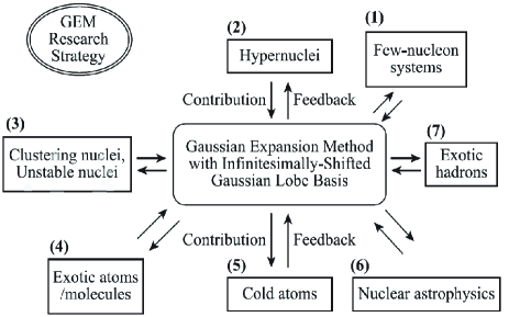
Figure 1: Research strategy for few-body physics with GEM.

Many important problems in physics can be addressed by accurately solving the Schrödinger equations for bound state, resonances and reaction processes in few-body (especially, 3- and 4-body) systems. It is of particular importance to develop various numerical methods for high-precision calculations of such problems. For this purpose, the present authors and collaborators proposed and have been developing the Gaussian expansion method for few-body systems Kamimura88 ; Kameyama89 ; Hiyama03 ; Hiyama12FEW ; Hiyama12PTEP .

Using the GEM, the present authors and collaborators have been studying many subjects in various research fields of physics. Our strategy for such studies is as follows: As shown in Fig. 1, we have our own calculation method GEM in the center and have been applying it to a variety of systems, such as (1) few-nucleon systems, (2) hypernuclei, (3) clustering nuclei and unstable nuclei, (4) exotic atoms/molecules, (5) cold atoms, (6) nuclear astrophysics and (7) exotic hadrons.

As indicated in Fig. 1 by arrows back to the center, we often obtained useful feedback from the calculation effort in each field, so that we further developed the GEM itself. We then applied the so-improved GEM to a new field where the present authors and collaborators had not enter before. We have been repeating this research cycle under this strategy.

The purpose of the present review paper is to explain i) high accuracy of GEM calculations and its reason, ii) wide applicability of GEM to various few-body systems, and iii) predictive power of GEM calculations.

In the case of bound states, the few-body Schrödinger equation is solved on the basis of the Rayleigh-Ritz variational principle; the total wave function is expanded in terms of the $L^{2}$-integrable basis functions by which Hamiltonian is diagonalized.

We employ few-body Gaussian basis functions that are spanned over all the sets of rearrangement Jacobi coordinates (for example, Eq. (2) for 3-body and Eq. (11) for 4-body systems). This construction of few-body basis functions using all the Jacobi coordinates makes the function space significantly larger than that spanned by the basis functions of single set of Jacobi coordinates.

In the authors’ opinion, a very useful set of basis functions along any Jacobi coordinate ${\bf r}$ is

$$e^{-\nu_{n}r^{2}}r^{l}\,Y_{lm}(\widehat{\bf r}),\;\;r_{n}=\nu_{n}^{\frac{1}{2}}=r_{1}a^{n-1}\;\;(n=1,...,N),$$

where the ranges are taken in geometric progression Kamimura88 ; and similarly for the other Jacobi coordinates. We refer to them as Gaussian basis functions.

The geometric progression $\{r_{n}\}$ is dense at short distances so that the description of the dynamics mediated by short range potentials can be properly treated. Moreover, though single Gaussian decays quickly, appropriate superposition of many Gaussians can decay accurately (exponentially) up to a sufficiently large distance. We show many example figures for 2-, 3- and 4-body cases in this paper (a reason why the ‘geometric progression’ works well is mentioned in Sec. II.2).

Use of Gaussians with complex ranges Hiyama03 ,

$$e^{-\eta_{n}r^{2}}r^{l}\,Y_{lm}(\widehat{\bf r}),\;\;\;\;\eta_{n}=(1\pm i\,\omega)\,\nu_{n},$$

makes the function space much wider than that of Gaussians with real ranges mentioned above since the former has oscillating part explicitly (cf. Sec. II.4). The new basis functions are especially suitable for describing wave functions having many oscillating nodes (cf. Figs. 45 and 46 in Appendix).

Therefore, in the study of few-body resonances using the complex-scaling method (for example, Aoyama2006 and cf. Sec. V.1), the complex-range Gaussian basis functions are specially useful since the resonance wave function in the method is highly oscillating when the rotation angles $\theta$ is large in the scaling $r\to r\,e^{i\theta}$.

Another important advantage of using real- and complex-range Gaussians is that calculation of the Hamiltonian matrix elements among the few-body basis functions can easily be performed Hiyama03 . This advantage is much more enhanced if one uses the infinitesimally-shifted Gaussian basis functions Hiyama94 ; Hiyama95u ; Hiyama03 introduced by the R.H.S. of

$$e^{-\nu_{n}r^{2}}r^{l}\,Y_{lm}({\widehat{\bf r}})=\!\lim_{\varepsilon\rightarrow 0}\frac{1}{(\nu_{n}\varepsilon)^{l}}\sum_{k=1}^{k_{\rm max}}\,C_{lm,k}\;e^{-\nu_{n}({\bf r}\,-\,\varepsilon{\bf D}_{lm,k})^{2}}$$

because the tedious angular-momentum algebra (Racah algebra) does not appear when calculating the few-body matrix elements (cf. Sec. II.5).

In the study of few-body scattering and reaction processes, we emply the Kohn-type variational principle to $S$-matrix Kamimura77 . The wave-function amplitude in the interaction region is expanded in terms of the few-body real- (complex-)range Gaussian basis functions constructed on all the sets of Jacobi coordinates. We consider the basis functions are nearly complete in the restricted region; examples will be discussed in Sec. V.2.

As long as the employed interactions among constituent particles (clusters) of the few-body system concerned are all well-established ones, accurate results by the GEM calculations are so reliable that we can use them to make a prediction before measurements about that system. If some members of such interactions are ambiguous (or not established), we first try to improve them phenomenologically in order to reproduce the existing experimental data for all the subsystems (possible combinations of the constituent members). Then, it is possible for the GEM calculation to make a prediction about the full system (cf. a strategy in our study of hypernuclear physics, Fig. 29, in Sec. IV.6). Examples of successful predictions by the GEM calculations will be presented in Sec. IV.

This article is organized as follows: Outline of the GEM framework is capitulated in Sec. II. Examples of high-precision GEM calculations are demonstrated in Sec. III. We review, in Sec. IV, examples of successful GEM predictions before measurements. Extension of GEM to few-body resonances and few-body reactions are presented in Sec. V. Summary is given in Sec. VI. In Appendix, we present several examples of 2-body GEM calculations in order to show the high accuracy of the real- and complex-range Gaussian basis functions, taking visible cases.

II GAUSSIAN EXPANSION METHOD (GEM) FOR FEW-BODY SYSTEMS

GEM has already been applied to various 3-, 4- and 5-body systems. In this section, we briefly explain the method taking the case of 3-body bound states for simplicity.

Applications to complex-scaling calculations for 3- and 4-body resonant states are shown Sec. V.1 and those to reactions are presented in Sec. V.2.

II.1 Use of all the Jacobi-coordinate sets

In GEM, solution to the Schrödinger equation for the bound-state wave function $\Psi_{JM}$ with the total angular momentum $J$ and its $z$-component $M$,

$$(H-E)\Psi_{JM}=0\,,$$ (1)

is obtained by diagonalizing the Hamiltonian in a space spanned by a finite number of $L^{2}$-integrable 3-body basis functions which are constructed on all the sets of Jacobi coordinates (Fig. 2).

Figure 2: Three sets of Jacobi coordinates of 3-body system. All of them are used in GEM calculations

The total wave function $\Psi_{JM}$ is written as a sum of component functions of all the 3 rearrangement channels

$$\Psi_{JM} = \sum_{\alpha=1}^{\alpha_{\rm max}}A_{\alpha}\,\Phi_{\alpha}^{(1)}({\bf r}_{1},{\bf R}_{1})+\sum_{\beta=1}^{\beta_{\rm max}}B_{\beta}\,\Phi_{\beta}^{(2)}({\bf r}_{2},{\bf R}_{2})$$ (2)

$$+ \sum_{\gamma=1}^{\gamma_{\rm max}}C_{\gamma}\,\Phi_{\gamma}^{(3)}({\bf r}_{3},{\bf R}_{3}),\qquad$$

where spins and isospins are omitted for simplicity. The 3-body basis functions are taken as

$$\!\!\!\!\!\!\!\!\Phi_{\alpha}^{(1)}({\bf r}_{1},{\bf R}_{1})\!=\!\phi_{n_{1}l_{1}}^{(1)}(r_{1})\,\psi_{N_{1}L_{1}}^{(1)}(R_{1})\Big{[}Y_{l_{1}}(\widehat{{\bf r}}_{1})\,Y_{L_{1}}(\widehat{{\bf R}}_{1})\Big{]}_{JM},$$

$$\!\!\!\!\!\!\!\!\Phi_{\beta}^{(2)}({\bf r}_{2},{\bf R}_{2})\!=\!\phi_{n_{2}l_{2}}^{(2)}(r_{2})\,\psi_{N_{2}L_{2}}^{(2)}(R_{2})\Big{[}Y_{l_{2}}(\widehat{{\bf r}}_{2})\,Y_{L_{2}}(\widehat{{\bf R}}_{2})\Big{]}_{JM},$$

$$\!\!\!\!\!\!\!\!\Phi_{\gamma}^{(3)}({\bf r}_{3},{\bf R}_{3})\!=\!\phi_{n_{3}l_{3}}^{(3)}(r_{3})\,\psi_{N_{3}L_{3}}^{(3)}(R_{3})\Big{[}Y_{l_{3}}(\widehat{{\bf r}}_{3})\,Y_{L_{3}}(\widehat{{\bf R}}_{3})\Big{]}_{JM},$$

(3)

where $\alpha$, $\beta$ and $\gamma$ specify

$$\alpha\equiv\{n_{1},l_{1},N_{1},L_{1}\}\>,\quad\beta\equiv\{n_{2},l_{2},N_{2},L_{2}\}\>,\quad$$

$$\gamma\equiv\{n_{3},l_{3},N_{3},L_{3}\}\>,$$ (4)

with $l,L$ denoting angular momenta and $n,N$ specifying radial dependence (namely, Gaussian ranges; see below). Energies $E$ and wave-function coefficients $A_{\alpha}$, $B_{\beta}$ and $C_{\gamma}$ are determined simultaneously by using the Rayleigh-Ritz variational principle, namely by diagonalizing the Hamiltonian using the basis functions.

If the three particles are identical particles, Eq. (2) is to be replaced by

$$\!\!\!\Psi_{JM}\!=\!\sum_{\alpha=1}^{\alpha_{\rm max}}\!A_{\alpha}\Big{[}\Phi_{\alpha}({\bf r}_{1},{\bf R}_{1})+\Phi_{\alpha}({\bf r}_{2},{\bf R}_{2})+\Phi_{\alpha}({\bf r}_{3},{\bf R}_{3})\Big{]}.$$

This construction of 3-body basis functions on all the sets of Jacobi coordinates makes the function space significantly larger than the case using the basis functions of single channel alone. Also it makes the non-orthogonality between the basis functions much less troublesome than in the single-channel case. These types of 3-body basis functions are particularly suitable for describing compact clustering between two particles along any $r_{c}~{}(c=1-3)$ and for a weakly coupling of the third particle along any $R_{c}$. We also emphasize that the 3-channel basis functions are particularly appropriate for systems composed of mass-different (distinguishable) particles.

II.2 Gaussians with ranges in geometric progression

Radial dependence of the basis functions $\phi_{nl}(r)$ and $\psi_{NL}(R)$ is taken as Gaussians (multiplied by $r^{l}\,$ and $R^{L}$) with ranges in geometric progression Kamimura88 ; Kameyama89 ; Hiyama03 :

$$\phi_{nl}(r) \!\!=\!\! N_{nl}\,r^{l}\>e^{-\nu_{n}r^{2}},$$

$$\nu_{n} \!\!=\!\! 1/r_{n}^{2}\;,\quad$$

$$r_{n} \!\!=\!\! r_{1}\,a^{n-1}\quad\>(n=1,...,n_{\rm max})$$ (5)

and

$$\psi_{NL}(R) \!\!=\!\! N_{NL}\,R^{L}\>e^{-\lambda_{N}R^{2}},$$

$$\lambda_{N} \!\!=\!\! 1/R_{N}^{2}\;,$$

$$R_{N} \!\!=\!\! R_{1}\,A^{N-1}\quad\>(N=1,...,N_{\rm max})$$ (6)

with the normalization constants $N_{nl}$ and $N_{NL}$.

The geometric progression is dense at short distances so that the description of the dynamics mediated by short range potentials can be properly treated. Moreover, though single Gaussian decays quickly, appropriate superposition of many Gaussians can decay accurately (exponentially) up to a sufficiently large distance. Good examples in 2-body systems are demonstrated in Figs. 42 and 44 in Appendix.

Even for 3- and 4-body systems, the Gaussian basis functions so chosen can describe accurately both short range correlations and long range asymptotic behavior simultaneously. Here, we emphasize that it is not necessary to introduce a priori the Jastrow correlation factor in the total wave function so as to describe the strong short-range correlations; it is enough for the purpose to use the Gaussian basis functions (5) and (6) as will be shown in successful results of Figs. 10 and 17 in 4-body systems.

A reason why the Gaussians with ranges in geometric progression work well may be stated as follows Hiyama12COLD-1 : The norm-overlap matrix elements, $N_{n,n+k}\,(k=0,...,n_{\rm max})$, between the basis functions is given as

$$N_{n,n+k}=\langle\phi_{n\,l}\,|\,\phi_{n+k\,l}\rangle=\left(\frac{2a^{k}}{1+a^{2k}}\right)^{l+3/2},$$ (7)

which shows that the overlap with the $k$-th neighbor is independent of $n$ and decreases gradually with increasing $k$ as illustrated in Fig. 3. We then expect that the coupling among the whole basis functions take place smoothly and coherently so as to describe properly both the short-range structure and long-range asymptotic behavior simultaneously.

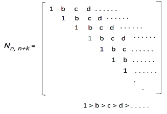
Figure 3: The norm-overlap matrix (7) in the case where the Gaussian ranges are given in geometric progression (5).

The Gaussian shape of basis functions makes the calculation of the Hamiltonian matrix elements easy even between different rearrangement channels. On the other hand, according to the experience by the authors, eigenfunctions of a harmonic-oscillator potential (namely, Gaussian times Laguerre polynomials) is not suitable for describing three- and more-body systems because of the tediousness in the coordinate transformation and in the many-dimensional integration when calculating the matrix elements. Also, it is difficult to describe a very weakly bound state that has a long-range tail since the long-range harmonic-oscillator eigenfunctions inevitably oscillate many times up to the tail region.

II.3 Easy optimization of nonlinear variational parameters

The setting of Gaussians with ranges in geometric progression as in Eqs. (5) and (6) enables us to optimize the ranges using a small number of free parameters; we recommend to take the sets {$n_{\rm max},r_{1},r_{n_{\rm max}}$} and {$N_{\rm max},R_{1},R_{N_{\rm max}}$} without using the ratios $a$ and $A$ which are given by $a=(r_{n_{\rm max}}/r_{1})^{1/(n_{\rm max}-1)}$ and $A=(R_{N_{\rm max}}/R_{1})^{1/(N_{\rm max}-1)}$.

Since the computation time by the use of the Gaussian basis functions is very short, we can take rather large number for ${n_{\rm max}}$ and ${N_{\rm max}}$, even more than enough. It is therefore satisfactory to optimize the Gaussian ranges {$r_{1},r_{n_{\rm max}},R_{1},R_{N_{\rm max}}$} using round numbers (cf. the 2-body examples in Appendix); this is due to the fact that small change of the ranges does not significantly change the function space since the space is already sufficiently wide by taking more-than-enough large numbers for ${n_{\rm max}}$ and ${N_{\rm max}}$.

In the calculation of the 3-nucleon bound states (³H and ³He) using a realistic $NN$ potential (AV14), the well-converged GEM calculation Kameyama89 took totally 3600 basis functions, but only the 3 cases of round-number sets $r_{1}=0.05,\>r_{n_{\rm max}}=15.0,\>R_{1}=0.3,\>R_{N_{\rm max}}=9.0$ fm,

$r_{1}=0.1\>\>,\>r_{n_{\rm max}}=15.0,\>R_{1}=0.3,\>R_{N_{\rm max}}=9.0$ fm,

$r_{1}=0.1\>\>,\>r_{n_{\rm max}}=10.0,\>R_{1}=0.3,\>R_{N_{\rm max}}=6.0$ fm

(depending on $l,L$ and spins; cf. Table I of Ref. Kameyama89 )

were so satisfactory that the binding energy converges with the 1-keV accuracy of four significant figures; as will be explained in Fig. 8 in Sec. III.2, this convergence with respect to the increasing number of angular-momentum channels is more rapid than that of the Faddeev-method calculations of the same problem.

Our method is quite transparent in the sense that all the nonlinear variational parameter employed can explicitly be listed in a small table. Therefore, one can examine the GEM results by making a check calculation with the same parameters. For example, even in a well-convered 4-body calculation in the cold-atom physics in Ref. Hiyama12COLD-1 by the present authors, all the nonlinear variational parameters for totally 23504 basis functions were listed in a small table of only 14 lines (Table V of that paper). This calculation will be introduced in Sec. III.5.

Good choice of the Gaussian ranges depends mostly on size and shape of the interaction and spatial extension of the system. But, to the authors’ opinion, slight experience is enough to master how to find such a choice thanks to the properties of the Gaussian basis functions mentioned above.

II.4 Complex-range Gaussian basis functions

In spite of many successful examples of the use of the Gaussian basis functions in the few-body calculations, it was hard to describe accurately highly-oscillatory wave functions having more than several nodes since the Gaussians themselves had no radial nodes.

To overcome this difficulty, the present authors proposed Hiyama03 new types of basis functions which have radial oscillations but tractable as easily as Gaussians; namely, Gaussians with complex ranges $\eta_{n}$ and $\eta^{*}_{n}$ instead of real range $\nu_{n}\,(n=1,...,n_{\rm max})$:

$$r^{l}e^{-\eta_{n}r^{2}}\>,\quad\;\;\eta_{n}=(1+i\,\omega)\,\nu_{n}\>,$$

$$r^{l}e^{-\eta_{n}^{*}r^{2}}\>,\quad\;\;\eta_{n}^{*}=(1-i\,\omega)\,\nu_{n}\>,$$ (8)

with $\nu_{n}$ in geometric progression as in (5). They are equivalent to the set

$$\quad r^{l}\>e^{-\nu_{n}r^{2}}{\rm cos}\>\omega\nu_{n}r^{2}\;=r^{l}(e^{-\eta_{n}r^{2}}+e^{-\eta_{n}^{*}r^{2}})/2\>,\quad$$

$$\quad r^{l}\>e^{-\nu_{n}r^{2}}{\rm sin}\>\omega\nu_{n}r^{2}\;=r^{l}(e^{-\eta_{n}r^{2}}-e^{-\eta_{n}^{*}r^{2}})/2i.\quad$$ (9)

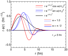
Figure 4: An example of the $l=0$ real-range and complex-range Gaussian basis functions (multiplied by $r$) of Eqs. (5) and (9) with $r_{n}=1/\sqrt{\nu_{n}}=5$ fm and $\omega=1.0$ and $\pi/2$. They are normalized to unity.

We refer to these oscillating functions (8) and (9) as complex-range Gaussians. From our experiences, we recommend to take simply $\omega=1$ or $\pi/2$ as well as adopting geometric progression for $\nu_{n}$. In order to compare visually the real-range and complex-range Gaussians, we plot an example of them in Fig. 4.

In Appendix A.6 for 2-body examples with a harmonic oscillator potential and a Coulomb potential, we show that use of the complex-range Gaussian basis functions makes it possible to represent oscillating functions having more than 20 radial nodes accurately (cf. Figs. 45 and 46).

Hamiltonian matrix elements between the complex-range Gaussians can be calculated with essentially the same computation program for the real-range Gaussians with some real variables replaced by complex ones; this is another advantage of the complex-range Gaussians.

Since the complex-range Gaussian basis functions makes the function space of few-body systems much wider than that with real-range Gaussians, applicability of GEM becomes much extended, for example, in Refs. Ohtsubo2013 ; Hiyama12COLD-1 ; Hiyama12COLD-2 ; Hiyama14COLD-3 ; Matsumoto03PS ; Matsumoto03CDCC ; Kamimura09 by the authors and collaborators.

II.5 Infinitesimally-shifted Gaussian-lobe (ISGL) basis functions

When we proceed to 4-body systems, calculation of the Hamiltonian matrix elements becomes much laborious especially when treating many spherical harmonic functions $Y_{lm}({\widehat{\bf r}})$ in the matrix element calculation. In order to make the 4-body calculation tractable even for complicated interactions, one of the present authors (E.H.) proposed the infinitesimally-shifted Gaussian-lobe (ISGL) basis functions Hiyama94 ; Hiyama95u ; Hiyama03 . The Gaussian function $r^{l}e^{-\nu_{n}r^{2}}Y_{lm}(\widehat{\bf r})$ is replaced by a superposition of infinitesimally-shifted Gaussians as

$$N_{nl}\,r^{l}e^{-\nu_{n}r^{2}}Y_{lm}({\widehat{\bf r}})=N_{nl}\,\lim_{\varepsilon\rightarrow 0}\;\frac{1}{(\nu_{n}\varepsilon)^{l}}$$

$$\times\sum_{k=1}^{k_{\rm max}}\;C_{lm,k}\;e^{-\nu_{n}({\bf r}\,-\,\varepsilon{\bf D}_{lm,k})^{2}}.$$ (10)

whose shift parameters $\{C_{lm,k},{\bf D}_{lm,k};\,k=1-k_{\rm max}\}$ are so determined that RHS is equivalent to LHS (see Appendix A.1 in Ref. Hiyama03 ).

We make similar replacement of the basis functions in all the other Jacobian coordinates. Thanks to the absence of the spherical harmonics, use of the ISGL basis functions makes the few-body Hamiltonian matrix-element calculation much easier with no tedious angular-momentum algebra (Racah algebra). When and how to take lim_ε→0 is important (see Appendix A.1 in Ref. Hiyama03 ). The Gaussian range $\nu_{n}$ can be taken to be complex $\eta_{n}$ as in Eq. (8) of the previous Sec. II.4.

Owing to this advantage, applicability of GEM becomes very wide in various research fields (cf. Fig. 1). Furthermore, use of ISGL basis functions make it easier to calculate few-body resonance states (cf. Sec. V.1) with the use of the complex-scaling method (cf. Ref. Aoyama2006 for a review) and to calculate few-body scattering states (cf. V.2) with the use of the Kohn-type variational principle to $S$-matrix Kamimura77 .

Here, we note a history about ’Gaussian-lobe basis functions’ (those not taking lim_ε→0 but using a small $\varepsilon$ in Eq. (10)). Such basis functions (whose shift parameters were different from ours) were advocated in 1960’s by several authors old-lobe on the basis of their simplicity to mimic $Y_{lm}({\widehat{\bf r}})$ with $l>0$. But, the functions have serious weakpoints; namely, computation with very small $\varepsilon$ makes the result easily suffer from heavy round-off error, whereas use of a not-very-small $\varepsilon$ meets an inevitable admixture of higher-order $Y_{l^{\prime}m}({\widehat{\bf r}})$ with $l^{\prime}>l$. Therefore, the functions were not utilized in actual research calculations and seemed soon forgotten when big computers came to real use.

But, some 30 years after, this difficulty was solved by one of the authors (E.H.) Hiyama94 ; Hiyama95u ; Hiyama03 by introducing the ISGL basis functions with properly taking lim_ε→0 after performing the analytical integration of the Hamiltonian matrix elements (see Appendix A3 and A.4 of Ref. Hiyama03 ); therefore, $\varepsilon$ does not appear in the computation program.

III Accuracy of GEM calculations

III.1 Muonic molecule in muon-catalyzed fusion cycle

The Gaussian expansion method was first proposed Kamimura88 in 1988 in the 3-body study of muonic molecule $dt\mu^{-}$ that appears in the cycle of muon-catalyzed $d$-$t$ fusion (for example, see Secs. 5 and 8 of Ref. Hiyama03 for a short survey, and Ref. Nagamine1998 for a precise review). The $d+t+\mu^{-}$ system is known to be a key to the possible energy production by the muon-catalyzed fusion ($\mu$CF) as shown in Fig. 5 for the essential part of the catalyzed cycle.

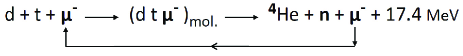
Figure 5: Essence of muon-catalyzed fusion cycle in which the 3-body $dt\mu^{-}$ molecule (at $J=v=1$ state) plays a key role to cause the fusion reaction $d+t\to~\!{}^{4}{\rm He}+n+17.4$MeV.

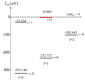
Figure 6: Theoretically predicted energy levels of the $dt\mu^{-}$ molecule. The near-threshold $J=v=1$ state (red) is important as the doorway to the muon catalyzed fusion (Fig. 5). This figure is reproduced from Ref. Kamimura88 .

Figure 7: Three Jacobi coordinates of the $dt\mu^{-}$ molecule in muon-catalyzed fusion cycle. Use of them all is suitable for describing the key $J=v=1$ state that is very weekly bound from the $(t\mu)_{1s}+d$ threshold Kamimura88 .

When negative muons $\mu^{-}$ are injected into the D₂/T₂ mixture, muonic molecules $dt\mu^{-}$ are resonantly formed in its $J=v=1$ state (Fig. 6) which is very loosely bound below the $(t\mu)_{1s}+d$ threshold and is the key to $\mu$CF. In order to analyze the observed data of the $dt\mu^{-}$ molecular formation rate, accuracy of 0.001 eV is required in the calculated energy of the $J=v=1$ state with respect to the $(t\mu)_{1s}+d$ threshold. Since the threshold energy is $-2711.242$ eV from the $d+t+\mu$ 3-body breakup threshold, the accuracy of 7 significant figures is required in the Coulomb 3-body calculation.

This difficult Coulomb 3-body problem was challenged during 1980’s by many theoreticians from chemistry, atomic/molecular physics and nuclear physics. The problem was finally solved in 1988 with the accuracy of 7 significant figures by three groups from USSR, USA and Japan giving the same energy of $-0.660$ eV from the $(t\mu)_{1s}+d$ threshold using different calculation methods; namely using a variational methods, respectively, with elliptic basis Korobov87 , with Slater geminal basis Alexander88 and with the GEM basis Kamimura88 (cf. Fig. 7 and Secs. II.1 and II.2).

An interesting point is the computation time to solve the 3-body Schödinger equation for single set of nonlinear variational parameters. In the two methods Korobov87 ; Alexander88 from chemistry and atomic/molecular physics, main difficulty comes from the severe non-orthogonality between their basis functions; diagonalization of the energy and overlap matrices required quadruple-precision computation ($\sim$30 decimal-digit arithmetics) and the computation time of $\sim\!$ 10 hours on the computers at that time.

On the other hand, GEM Kamimura88 needed only 3 minutes. This rapid computation is owing to the use of Gaussian basis functions, which are spanned over the 3 rearrangement channels and have the ranges in geometrical progressions. Use of them suffers little from the trouble of severe non-orthogonality between large-scale ($\sim$2000) basis functions. Therefore the method works entirely in double-precision ($\sim$14 decimal-digit arithmetics) on supercomputers at that time. Another reason was that the function form of the basis functions is particularly suitable for vector-type supercomputers.

III.2 3-nucleon bound states (³H and ³He)

One of the best tests of three-body calculation method is to solve three-nucleon bound states (³H and ³He) using a realistic $NN$ force. This test was done for GEM in Ref. Kameyama89 using the AV14 force Wiringa84 and in Ref. Kamimura90 using the AV14 force plus the Tucson-Melborne (TM) 3-body force Coon79 . We shortly review them here.

In practical calculations, we have to truncate the angular-momentum space of the basis functions. It is to be stressed, however, that the interaction is not truncated in the angular-momentum space in the GEM calculations. In the calculation described below we restrict the orbital angular momenta $(l,L)$ of the spatial part of the basis functions in Eqs. (5) and (6) to $l+L\leq 6$, which results in 26 types of the $LS$-coupling configurations. We refer to such configurations as 3-body angular-momentum channels. The 26 channels employed in our calculation are listed in Table I of Ref. Kameyama89 together with the Gaussian parameters. It is to be emphasized that all the nonlinear variational parameters of the GEM calculation are explicitly listed in such a small table; in principle, one can examine the calculated results by using the same parameters.

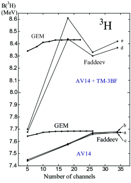
Figure 8: Convergence of the binding energies of ³H calculated by the present method Kameyama89 ; Kamimura90 and by the Faddeev method with respect to the number of the three-body channels. Interactions used are AV14 (lower lines) and AV14+TM-3BF (upper lines). Ref. Chen85 for line c, Ref. Ishikawa86 for b and e, and Ref. Sasakawa88 for a, d, f, g. This figure is taken from Ref. Kameyama89 ; Kamimura90 , where a similar figure for ³He is given.

Convergence of the binding energy of ³H with respect to the number of the 3-body angular-momentum channels is illustrated in Fig. 8. The results shown are those given by GEM in Refs. Kameyama89 ; Kamimura90 some $\sim$ 30 years ago together with those given by the Faddeev calculations at that time. The convergence is very rapid in GEM.

We note that one of the reasons for such a rapid convergence in the GEM framework comes from the fact that the interaction is treated without partial-wave decomposition (namely, no truncation in the angular-momentum space). This is a difference from the Faddeev-method calculations and is also pointed out in §2.2 of Ref. Gibson93 by Payne and Gibson.

III.3 Benchmark test calculations of 4-nucleon (⁴He) ground and second $0^{+}$ states

III.3.1 ⁴He ground state

Calculation of the 4-nucleon bound state (⁴He) using realistic $NN$ force is useful for testing methods and schemes for few-body calculations. In 2001, a very severe benchmark test calculation of the 4-body bound state was performed in Ref. Kamada01 by 18 authors, including the present authors, from seven research groups with the use of their own efficient calculation methods, namely, the Faddeev-Yakubovsky equation method (FY), the Gaussian expansion method (GEM), the stochastic variational method (SVM), the hyperspherical harmonic variational method (HH), the Green’s function Monte Carlo (GFMC) method, the no-core shell model (NCSM) and effective interaction hyperspherical harmonic method (EIHH). Those different calculation methods were explained briefly in the paper Kamada01 .

They used the $NN$ realistic force, AV8^′ interaction AV8P97 (consisting of central, spin-orbit and tensor forces), and compared the calculated energy eigenvalues and some wave function properties of the ⁴He ground state.

The present authors (GEM) employed 4-body Gaussian basis functions spanned over the full 18 sets of Jacobi coordinates (composed of the K-type and H-type ones) as shown in Fig. 9.

Figure 9: K-type and H-type Jacobi coordinates for the 4-nucleon systems. Antisymmetrization of the 4 particles generates the Jacobi coordinate sets $c=1,...,12$ (K-type) and $c=13,...,18$ (H-type). See Fig. 18 of Ref. Hiyama03 for explicit figures of the 18 sets.

In the GEM approach, the most general 4-nucleon wave function (with $J$ for the total angular momentum and $T$ for the isospin) is written as a sum of the component functions in the K- and H-type Jacobi coordinates employing the $LS$ coupling scheme:

$$\!\!\!\Psi_{JM,TT_{z}}=\!\sum_{\alpha}C^{({\rm K})}_{\alpha}\Phi^{({\rm K})}_{\alpha}+\!\sum_{\alpha}C^{({\bf H})}_{\alpha}\Phi^{({\rm H})}_{\alpha},$$ (11)

where the antisymmetrized 4-body basis functions $\Phi^{({\rm K})}_{\alpha}$ and $\Phi^{({\rm H})}_{\alpha}$ (whose suffix $JM,TT_{z}$ are dropped for simplicity) are described by

$$\Phi^{({\rm K})}_{\alpha}\!\! = \!\!{\cal A}\left\{\Big{[}\big{[}[\phi_{nl}^{({\rm K})}({\bf r}_{\rm K})\varphi_{\nu\lambda}^{({\rm K})}(\mbox{\boldmath$\rho$}_{\rm K})]_{\Lambda}\;\psi_{NL}^{({\rm K})}({\bf R}_{\rm K})\big{]}_{I}\right.$$ (12)

$$\quad\times\big{[}[\chi_{s}(12)\chi_{1/2}(3)]_{s^{\prime}}\chi_{1/2}(4)\big{]}_{S}\Big{]}_{JM}$$

$$\quad\times\left.\big{[}[\eta_{t}(12)\eta_{1/2}(3)]_{t^{\prime}}\eta_{1/2}(4)\big{]}_{TT_{z}}\right\},$$

$$\Phi^{({\rm H})}_{\alpha}\!\! = \!\!{\cal A}\left\{\Big{[}\big{[}[\phi_{nl}^{({\rm H})}({\bf r}_{\rm H})\varphi_{\nu\lambda}^{({\rm H})}(\mbox{\boldmath$\rho$}_{\rm H})]_{\Lambda}\;\psi_{NL}^{({\rm H})}({\bf R}_{\rm H})\big{]}_{I}\right.$$ (13)

$$\quad\times\big{[}\chi_{s}(12)\chi_{s^{\prime}}(34)\big{]}_{S}\Big{]}_{JM}$$

$$\quad\times\left.\big{[}\eta_{t}(12)\eta_{t^{\prime}}(34)\big{]}_{TT_{z}}\right\},$$

with $\alpha\equiv\{nl,\nu\lambda,\Lambda,NL,I,s,s^{\prime},S,t,t^{\prime}\}$. $\cal{A}$ is the 4-nucleon antisymmetrizer. Parity of the wave function is given by $\pi=(-)^{l+\lambda+L}$. The $\chi$’s and $\eta$’s are the spin and isospin functions, respectively. The spatial basis functions $\phi_{nlm}({\bf r})$, $\varphi_{\nu\lambda\mu}(\mbox{\boldmath$\rho$})$ and $\psi_{NLM}({\bf R})$ are taken to be Gaussians multiplied by spherical harmonics:

$$\phi_{nlm}({\bf r})=N_{nl}\,r^{l}\>e^{-(r/r_{n})^{2}}\>Y_{lm}({\widehat{\bf r}})\;,$$

$$\varphi_{\nu\lambda\mu}(\mbox{\boldmath$\rho$})=N_{\nu\lambda}\,\rho^{\lambda}\>e^{-(\rho/\rho_{\nu})^{2}}\>Y_{\lambda\mu}({\widehat{\mbox{\boldmath$\rho$}}})\;,$$ (14)

$$\psi_{NLM}({\bf R})=N_{NL}\,R^{L}\>e^{-(R/R_{N})^{2}}\>Y_{LM}({\widehat{\bf R}})\;.$$

It is important to postulate that the Gaussian ranges lie in geometric progression as in Eqs. (5) and (6).

Table 1: Calculated results for some of ⁴He properties (binding energy, r.m.s radius and $D$-state probability) by seven methods of calculation. Reproduced from Ref. Kamada01 .

Method	B.E. (MeV)	$\sqrt{\langle r^{2}\rangle}$ (fm)	$D$ (%)
FY	$25.94(9)$	1.485(3)	13.91
GEM	$25.90$	1.482	13.90
SVM	$25.92$	1.486	13.91
HH	$25.90(1)$	1.483	13.91
GFMC	$25.93(2)$	1.490(5)	$\;\;-$
NCSM	$25.80(20)$	1.485	12.98
EIHH	$25.944(10)$	1.486	13.89(1)

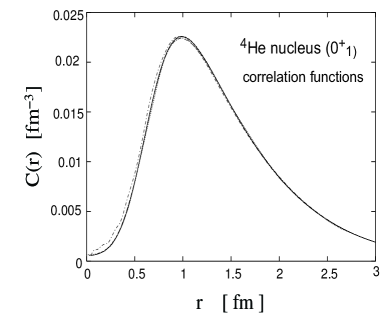
Figure 10: Correlation functions (two-body density) of ⁴He, $C(r)\!=\!\langle\Psi|\delta({\bf r}{\rm-}{\bf r}_{12})|\Psi\rangle$, in the different calculational schemes: FY, GEM, SVM, HH, and NCSM (overlapping curves) and EIHH(dashed-dotted curve), except GFMC. Taken from Ref. Kamada01 .

The work of benchmark test Kamada01 demonstrated that the Schrödinger equation for the 4-nucleon ground state can be handled very reliably by the different seven methods, leading to very good agreement between them in the calculated results (some examples are shown in Table 1 and Fig. 10). This fact is quite remarkable in view of the very different techniques of calculation and the complexity of the nuclear force chosen.

III.3.2 ⁴He second $0^{+}$ state

Soon after the benchmark test, the present authors succeeded Hiya04SECOND , using the same GEM framework, in extending the ⁴He ground-state calculation to the second $0^{+}$ state that has a very loose spatial distribution compared with the compact ground state. It can be a severe test for few-body calculation methods to describe simultaneously the two $0^{+}$ states that have very different properties.

Table 2: (Upper) Calculated and observed binding energies of ³H, ³He, ⁴He$(0^{+}_{1})$ and ⁴He$(0^{+}_{2})$. The 4-body GEM calculation Hiya04SECOND takes the AV8^′ and Coulomb potential plus a phenomenological 3-body force. (Lower) Calculated probability percentages of the $S,P$ and $D$ states, which are nearly the same between ³H (³He) and ⁴He$(0^{+}_{2})$. This table is reproduced from Ref. Hiya04SECOND .

B.E. (MeV)	$\;\;{}^{3}$H	3He		4He $(0^{+}_{1})$	4He $(0^{+}_{2})$
GEM	8.41	7.74		28.44	8.19
EXP	8.48	7.72		28.30	8.09
$P_{S}$ (%)	90.96	90.99		85.54	91.18
$P_{P}$ (%)	0.08	0.08		0.38	0.08
$P_{D}$ (%)	8.97	8.93		14.08	8.74

First, in order to reproduce simultaneously the observed binding energies of ³H, ³He and ⁴He$(0^{+}_{1})$ before entering the ⁴He$(0^{+}_{2})$ state, we introduced a phenomenological 3-body force (Eq. (3.1) of Ref. Hiya04SECOND ) in addition to the AV8^′ and Coulomb forces. A good agreement for the former three states was obtained as shown Table LABEL:table:3n-4n-energy (upper part). At the same time, the calculated binding energy of the ⁴He$(0^{+}_{2})$ state was found to reproduce the observed one well.

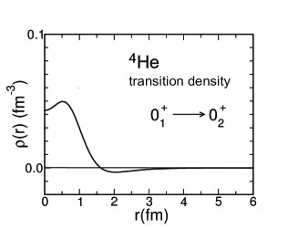
Figure 11: Mass densities of the $0^{+}_{1}$ and $0^{+}_{2}$ states of ⁴He (upper) and the transition density between them (lower). Taken from Ref. Hiya04SECOND .

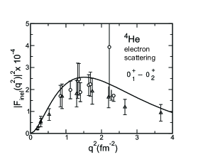
Figure 12: A GEM 4-body calculation Hiya04SECOND (solid line) of the electron-scattering form factor for ${}^{4}{\rm He}(e,e^{\prime})^{4}{\rm He}(0^{+}_{2})$, which is compared with the available experimental data (for references, see Ref. Hiya04SECOND ) in good agreement. Taken from Ref. Hiya04SECOND .

The lower part of Table LABEL:table:3n-4n-energy gives calculated probability percentages of the $S,P$ and $D$ components. Interestingly, they are almost the same between ³H (³He) and ⁴He$(0^{+}_{2})$. This means that the loosely coupled ${}^{3}{\rm H}+p$ (${}^{3}{\rm He}+n$) configuration is dominant in the second $0^{+}$ state.

As shown in Fig. 11 (upper), distribution of the calculated mass densities are quite different between the $0^{+}_{1}$ and $0^{+}_{2}$ states as expected. The transition density between the two states in Fig. 11 (lower) provides, via a Fourier transformation, the inelastic electron-scattering form factor of ⁴He($e,e^{\prime})^{4}$He($0^{+}_{2}$). Therefore, comparison of the form factor with the observed one can be another severe test of the GEM calculation. We reproduced, for the first time using realistic $NN$ interaction, the observed ⁴He($e,e^{\prime})^{4}$He($0^{+}_{2}$) data as shown in Fig. 12.

We note that our results for the second $0^{+}$ state can be used in another new benchmark test calculation (the result of Table LABEL:table:3n-4n-energy was reproduced by Ref. WHoriuchi ).

III.4 Determination of antiproton mass by GEM

The mass of antiproton has been believed to be the same as the mass of proton, but there was no precise experimental information on it before 2000. In the 1998 edition of Particle Listings Listing1998 , the Particle Data Group gave no recommended value of the antiproton mass.

In the Particle Listings 2000 Listing2000 , a recommended value was given for the first time; the relative deviation of the antiproton mass from the proton mass ($|m_{\bar{p}}-m_{p}|/m_{p})$ is within $5\times 10^{-7}$.

This value was derived by a collaboration of experimental and theoretical studies of the antiprotonic helium atom (${\bar{p}}$He⁺) composed of He${}^{2+}+{\bar{p}}+e^{-}$, namely, by the high-resolution laser spectroscopy experiment at CERN by Torii et al. Torii99 and the precision 3-body calculations by Kino, Kudo and one of the authors (M.K.) Kino98 ; Kino99 (summarized in Sec. 6 of Ref. Hiyama03 together with Refs. Kino00 ; Kino01 ).

The experiment for the transition between the highly-excited metastable states with $(J,v)=(34,2)$ and $(J,v)=(33,2)$ gave the wave length $\lambda_{\rm EXP}=470.7220(6)$ nm (Fig. 13). But, it is to be noted that this value of $\lambda_{\rm EXP}$ itself does not directly give any information on the antiproton mass. In Ref. Kino99 , the data were analyzed so that the mass of antiproton could be derived.

In the following, we briefly explain the GEM calculation of the antiprotonic helium atom that is called atomcule since it has two different facets, i) atomic picture of a positive-charge nucleus (He²⁺) plus two negative-charge particles and ii) molecular picture of two heavy particles (He²⁺ and ${\bar{p}}$) plus an electron (Fig. 14).

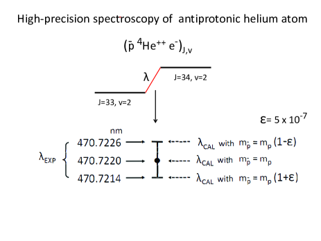
Figure 13:   Relative difference of the antiproton mass $(m_{\bar{p}})$ from the proton mass ($m_{p}$), $\varepsilon=|m_{\bar{p}}-m_{p}|/m_{p}$, was determined by the comparison between the spectroscopic experimental data ($\lambda_{\rm EXP}$) Torii99 and the 3-body GEM calculation ($\lambda_{\rm CAL}$) Kino99 on the antiprotonic He atom (${\bar{p}}$He⁺). This gave $\varepsilon=5\times 10^{-7}$.

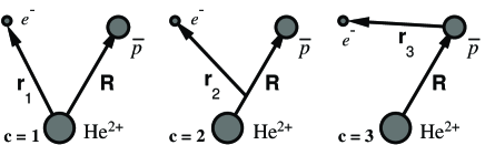
Figure 14: Three rearrangement channels for the antiprotonic helium atom (He${}^{2+}+e^{-}+{\bar{p}}$). Channels $c=1$ and $c=2$ are suitable for describing the atomic picture and the molecular picture, respectively, of this system. Channel $c=3$ is good at treating the correlation between the electron and the antiproton explicitly. The mass-polarization term in the kinetic-energy operator due to this choice of the coordinates is exactly treated.

This complicated system has difficult but important issues as follows:

1) The two different facets mentioned above should be well described simultaneously (GEM takes the channels $c=1$ and 2 in Fig. 14).

2) The excited states concerned are not true bound states but so-called Feshbach resonances (GEM takes the complex-scaling method of Sec. V.1).

3) Quantum number of the total angular momentum concerned is as high as $J\sim 30-40$.

4) The inter-nuclear motion between the helium nucleus ($Z=+2$) and the antiproton ($Z=-1$) can not be treated adiabatically when they are close to each other (GEM is a non-adiabatic method).

5) The correlation between the electron and the antiproton must be accurately taken into account (GEM takes the channel $c=3$ explicitly).

6) Accuracy of 8 significant figures in the transition energy (10 figures in eigenenergies before subtraction) is required to compare with the laser experiment of the transition frequency.

All of the issues 1) through 6) are difficult, but the GEM calculation in Refs. Kino98 ; Kino99 cleared them all and made it possible to determine the antiproton mass recommended in Particle Listings 2000. We explain how to determine the antiproton mass using the eigenenergies given by the 3-body GEM calculation.

The authors of Ref. Kino99 showed that the central value of $\lambda_{\rm EXP}$ was reproduced by $\lambda_{\rm CAL}$ when taking $m_{\bar{p}}=m_{p}$ and that the upper and lower bounds of $\lambda_{\rm EXP}$ were respectively reproduced by assuming (cf. Fig. 13)

$$m_{\bar{p}}=(1\mp\varepsilon)m_{p}\quad\mbox{with}\quad\varepsilon=5\times 10^{-7}.$$ (15)

Here, the relativistic and QED corrections were taken into account; the corrections are $\sim 10^{-5}$ times smaller than the non-relativistic result.

The authors of Ref. Kino99 then considered – even if the antiproton mass $m_{\bar{p}}$ is deviated from $m_{p}$, the calculated wavelength $\lambda_{\rm CAL}$ using the $m_{\bar{p}}$ should be within the experimental error (namely, the experimental error is fully attributed to the ambiguity of the antiproton mass). Then, they reached the conclusion

$$(1-\varepsilon)m_{p}<m_{\bar{p}}<(1+\varepsilon)m_{p}$$ (16)

namely,

$$\frac{|m_{\bar{p}}-m_{p}|}{m_{p}}<\varepsilon=5\times 10^{-7},$$ (17)

which was cited in Particle Listings 2000 Listing2000 ; it was commented that this can be a test of $CPT$ invariance. GEM is so accurate as to contribute to such a fundamental issue. More about the ${\bar{p}}$He⁺ atom and $m_{\bar{p}}$ is given in Sec. IV.1.

III.5 Calculation of ⁴He-atom tetramer in cold-atom physics (Efimov physics)

III.5.1 Universality in few-body systems

An essential issue in the cold-atom physics (Efimov physics) may be stated as that particles with short-range interactions and a large scattering length have universal low-energy properties that do not depend on the details of their structure or their interactions at short distances (see, for example, Ref. Braaten2006 for a review). Such an pair-interaction is often called ‘resonant interaction’ since the interacting pair has a resonance or a bound state that is located very closely to the 2-body breakup threshold. Typical examples are the interaction between $\alpha$ particles (⁴He nucleus) and that between ⁴He atoms.

The level structure of ⁴He-atom dimer, trimer and tetramer is illustrated in Fig. 15; calculation of all of the levels using the realistic interactions between ⁴He atoms was performed, for the first time, by the present authors Hiyama12COLD-1 as discussed below. It is interesting to note that this level structure is very similar to that of the lowest-lying $0^{+}$ states in 2$\alpha$ (⁸Be), 3$\alpha$ (¹²C) and 4$\alpha$ (¹⁶O) nuclei though the scale of the two interactions is quite different to each other; this is due to the universality mentioned above.

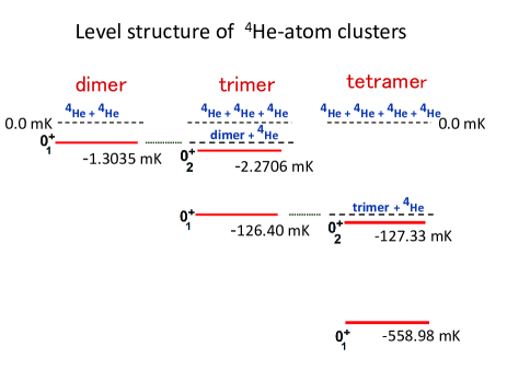
Figure 15: Level structure of ⁴He-atom clusters calculated by the present authors Hiyama12COLD-1 using the realistic interaction between ⁴He atoms. Note that this structure is quite resemble to that of the 2-, 3- and 4-$\alpha$ clusters (⁸Be, ¹²C and ¹⁶O nuclei) due to the universality in Efimov physics.

Theoretical study of energies and wave functions of the 3- and 4-body ⁴He-atom clusters is one of the fundamental subjects in the cold-atom physics since the realistic interaction between ⁴He atoms is a prototype and well-studied interaction in the Efimov physics. The interaction has an extremely strong short-range repulsive core due to the Pauli principle between electrons ($\sim 10^{6}$ K in height) followed by a weak attraction by the van der Waals potential ($\sim-10$ K in depth) (see Fig. 43 in Appendix A.5 for a typical LM2M2 potential LM2M2 ). The interaction has a large scattering length ($\sim 100\,$Å) much larger than the interaction range ($\sim 5\,$Å) and supports a very shallow bound states ($\sim-0.001$ K).

III.5.2 Difficulty in calculating ⁴He-atom tetramer

Until the energy levels of Fig. 15 were reported Hiyama12COLD-1 , a long standing problem in the study of ⁴He-atom clusters was the difficulty in performing a reliable 4-body calculation of the very-weakly-bound excited state $(\mbox{$v=1,\,$}0^{+}_{2})$ of ⁴He-tetramer in the presence of extremely strong short-range repulsive core; one has to describe accurately both the short-range structure ($\lesssim 5\!$ Å) and the long-range asymptotic behavior (up to $\sim 1000\,$Å).

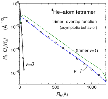
Figure 16: Good asymptotic behavior, up to $\sim 1000$ Å, of the overlap function $O_{v}(R_{k})\!\!=\!\!\langle\Psi_{3,v_{3}=0}|\Psi_{4,v}\rangle$, multiplied by $R_{k}$, between the trimer ground state $(v_{3}=0)$ and the tetramer states $(v=0,1)$. Open circles represent the exact asymptotic behavior. The green dash-dotted line is the same quantity between trimer excited state and dimer. Taken from Ref. Hiyama12COLD-1 .

The authors of Ref. Carbonell (2006), who used the 4-body Faddeev-Yakubovsky method, said “A direct calculation of the ⁴He-tetramer excited state represents nowadays a hardly realizable task”; instead, they derived the excited-state binding energy by an extrapolation from a low-energy atom-trimer scattering $S$-matrix.

However, this difficult problem was solved by the present authors Hiyama12COLD-1 (2012) with a 4-body GEM calculation. We employed the same set of all the 4-body Jacobi-coordinates of Fig. 9 as used in the 4-nucleon study in Sec. III.3. The energy of the ⁴He-tetramer excited state was obtained as $E=-0.00093$ K with respect to the atom-trimer threshold (Fig. 15). In this calculation we took 23504 4-body basis functions whose nonlinear parameters are all listed in a small table of 14 lines (Table V of Ref. Hiyama12COLD-1 ) as pointed out in Sec. II.3.

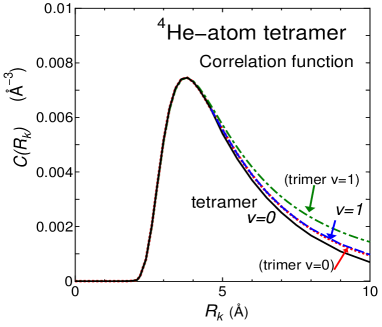
Figure 17: Short-range structure of the pair correlation function $C(r)\!=\!\langle\Psi|\delta({\bf r}{\rm-}{\bf r}_{12})|\Psi\rangle$ of the ⁴He tetramer calculated with the 4-body GEM Hiyama12COLD-1 . The black solid line stands for the tetramer ground $(v=0)$ state and the blue dashed line for the excited $(v=1)$ state. For the sake of comparison, additionally shown are the red dotted line for the trimer ground state and the green dash-dotted line for the trimer excited state. That for dimer nearly overlaps with the green line. The lines are normalized to the peak value of the black line. It is striking that the same shape of the short-range correlation ($r\lesssim 5$ Å ) appears in all the states. Taken from Ref. Hiyama12COLD-1 .

The excited-state wave function exhibits correct asymptotic behavior up to $\sim\!1000$Å as seen in Fig. 16 for the overlap function between the tetramer excited state and the trimer ground state. In Fig. 17, it is interesting to see that behavior of the extremely-strong short-range correlations ($\lesssim 5\!$ Å) in the tetramer has almost the same shape as in the dimer and in the trimer. This justifies the assumption in some literature calculations that the Jastrow correlation factor is a priori employed in few-body wave functions so as to treat the strong repulsive force between the interacting pair.

III.5.3 Efimov scenario: CAL versus EXP

Here, we do not intend to enter the details of the cold-atom physics, but our calculations mentioned below are closely related to the keypoint of the physics as follows:

Surprisingly to nuclear physicists, strength (in other word, scattering length) of the interaction between some ultra-cold atoms, such as ¹³³Cs, ⁸⁵Rb and ⁷Li at $\mu$K, can be changed/tuned by a magnetic field from outside utilizing Feshbach resonances of the atom pair located near the threshold. Realization of this experimental technics (at $\sim$ 2006) has very much developed the cold-atom physics (Efimov physics). One can investigate the structure change (called Efimov scenario) of the atom clusters (dimer, trimer, tetramer,…) as a function of the scattering length of the atom-atom interaction.

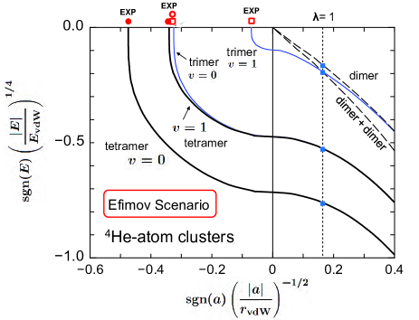
Figure 18: Efimov scenario (spectrum) for the ⁴He-atom clusters calculated in Ref. Hiyama14COLD-3 with the realistic ⁴He-⁴He potentials. The thick solid curves represent the tetramer spectrum that is the scaled tetramer energy $E_{4}^{(v)}/E_{\rm vdW}$ as a function of the scaled-inverse scattering length $(a/r_{\rm vdW})^{-1}$ for the ground $(v=0)$ and excited $(v=1)$ states. The thin solid blue curves denote the trimer spectrum. The critical scattering lengths where the tetramer energies $E_{4}^{(0)}$ and $E_{4}^{(1)}$ cross the 4-atom threshold are named as $a_{-}^{(4,0)}$ and $a_{-}^{(4,1)}$, respectively; the corresponding observed values for the ¹³³Cs, ⁸⁵Rb and ⁷Li tetramers are given by red circles, and similarly for trimers by red boxes (see the text). Taken from Ref. Hiyama14COLD-3 .

In Fig. 18, the present authors calculated Hiyama14COLD-3 the Efimov scenario (essentially, an energy spectrum of $E$ versus scattering length $a$) for the first time using realistic atom-atom potential (here, the ⁴He-atom potential). Following the literature, we have drawn $(|E|/E_{\rm vdW})^{1/4}$ versus $(|a|/r_{\rm vdW})^{-1/2}$ so that all the curves are graphically represented on the same scale. The scattering length $a$ and the energy $E$ are scaled with the van der Waals length $r_{\rm vdW}\,(=5.08\,a_{0}$) and energy $E_{\rm vdW}=\hbar^{2}/mr_{\rm vdW}^{2}\,(=1.677$ K), respectively. The dashed curve shows the dimer energy.

In Fig. 18, the scattering length $a$ are tuned by changing the factor $\lambda$ which is multiplied to the realistic ⁴He-⁴He interaction:

$$\big{[}\,T+\sum_{1=i<j}^{A}\lambda\,V(r_{ij})-E_{A}\,\big{]}\,\Psi_{A}=0,$$ (18)

where $T$ is the kinetic energy and $A(=2,3,4)$ is the number of ⁴He-atom clusters concerned.

The vertical dotted line stands for the physical value $\lambda=1$. The blue circles on the line indicate the energy levels that are illustrated in Fig. 15 with red lines; namely, from the top, they are the energies of the dimmer, the trimer excited state, the trimer ground state (overlapping with the circle for the tetramer excited state) and the tetramer ground state.

The states move to the left as $\lambda$ decreases ($a^{-1}$ decreases). In the region $a^{-1}<0$, there is no 2-body bound state, but the blue curves for the trimer show that the 3-body system is bound (this is a general form of the so-called Borromine states).

The critical scattering lengths where the tetramer energies $E_{4}^{(0)}$ and $E_{4}^{(1)}$ (black solid curves) cross the 4-atom threshold (the $E=0$ line) are named as $a_{-}^{(4,0)}$ and $a_{-}^{(4,1)}$, respectively, and their values scaled with $r_{\rm vdW}$ are summarized in Table II in Ref. Hiyama14COLD-3 together with the corresponding observed values (red circles in Fig. 18 for ¹³³Cs, ⁸⁵Rb and ^6,7Li), and similarly for the trimers (red boxes for the corresponding observed values).

It is striking that the GEM calculation Hiyama14COLD-3 of the critical scattering lengths of the trimer and tetramer using the realistic potentials of ⁴He atoms explains consistently the above-mentioned corresponding observed values that are the heart of cold-atom (Efimov) physics.

IV Successful predictions by GEM calculations

As mentioned in the previous section, applicability of GEM to various few-body calculations with high accuracy has been much improved. Therefore, it became possible to make theoretical prediction before measurement (as long as interactions employed are reliable); some successful examples are reviewed below.

IV.1 Prediction of energy levels of antiprotonic He atom

As mentioned in Sec. III.4, the precise 3-body GEM calculation of the antiprotonic helium atom (${\bar{p}}$He⁺=He${}^{2+}+{\bar{p}}+e^{-}$) contributed to the first determination of the antiproton mass in Particle Listings 2000. Since then, a lot of transitions between excited states of the atom were observed by CERN’s laser experiment. But, due to very expensive cost of the precise sub-ppm laser-scan search of the transition energy $\Delta E$, GEM was requested to predict $\Delta E$ before measurements.

A typical example of the transition frequency ($\nu$) by the GEM prediction Kino01 and the experimental result Hori01 is listed in Table LABEL:table:pbar-atom-energy. So accurate is the theoretical prediction using GEM.

Table 3: Comparison of the prediction by GEM Kino01 with the CERN experiment Hori01 about the transition frequencies between some levels of the antiprotonic helium atom (${\bar{p}}$He⁺).

$(J,v)-(J^{\prime},v^{\prime})$		$(32,0)-(31,0)$		$(33,1)-(32,1)$
		$\quad\nu$ (GHz)		$\quad\nu$ (GHz)
GEM		1 012 445.559		804 633.127(5)
EXP		1 012 445.52(17)		804 633.11(11)

On the basis of this comparison, in the same way as in Sec. III.4, a relative deviation of the antiproton mass from the proton mass $|m_{\bar{p}}-m_{p}|/m_{p}<6\times 10^{-8}$ was reported in the 2002 edition of Particle Listings Hagiwara02 .

The laser spectroscopy of metastable antiprotonic helium atoms is a pioneering work toward anti-matter science. We see that the GEM calculations was providing suggestive, helpful predictions for anti-matter science in a preliminary stage.

IV.2 Prediction of shrinkage of hypernuclei

When a $\Lambda$ particle is injected into a nucleus, how modified is structure of the nucleus? There is no Pauli principle acting between $\Lambda$ and nucleons in the nucleus. Therefore, the $\Lambda$ particle can reach deep inside, and attract the surrounding nucleons towards the interior of the nucleus (this is called ”gluelike role” of $\Lambda$ particle). However, how do we observe the shrinkage of the nuclear size by the $\Lambda$ participation? In the work of Ref. Motoba83 based on the microscopic $\alpha+x+\Lambda$ 3-cluster model $(x=d,t,^{3}$He) for light $p$-shell hypernuclei together with the $\alpha+x$ 2-cluster model for the nuclear core, the reduction of the nuclear size was discussed in relation to the reduction of the $B(E2)$ strength which is proportional to the fourth power of the distance between the clusters.

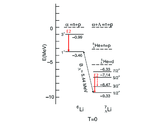
Figure 19: $E2$ transitions in ⁶Li and in ${}^{7}_{\Lambda}$Li that are used to discuss about the shrinkage of hypernucleus.

Figure 20: Jacobian coordinates of the ${\rm core}+N_{1}+N_{2}$ system where the core is hypernucleus ${}^{5}_{\Lambda}{\rm He}$ and $N_{1}$($N_{2}$) is a nucleon.

More precisely, in Ref. Hiyama99 , we explicitly suggested measurement of $B(E2;5/2^{+}_{1}\rightarrow 1/2^{+}_{1})$ in ${}^{7}_{\Lambda}$Li (Fig. 19) and proposed a prescription to derive hypernuclear size with the aid of the empirical values of $B(E2;3^{+}_{1}\rightarrow 1^{+}_{1})$ and the size of the ground state of ⁶Li. We also noted that another decay branch $B(E2;5/2^{+}_{1}\rightarrow 3/2^{+}_{1})$ is negligibly small, measurement of the lifetime of the ${}^{7}_{\Lambda}$Li$(5/2^{+}_{1})$ state can give the $B(E2;5/2^{+}_{1}\rightarrow 1/2^{+}_{1})$. Afterwards, the experiment by Ref. Tanida01 was performed and the result was compared with our prediction on the size of ${}^{7}_{\Lambda}$Li.

We employed a microscopic ${}^{5}_{\Lambda}{\rm He}+n+p$ 3-body model for ${}^{7}_{\Lambda}$Li Hiyama99 . It was examined in Ref. Hiyama96-5L that the ${}^{5}_{\Lambda}{\rm He}$ is a good cluster. The total 3-body wave function is constructed on the Jacobian coordinates of Fig. 20 in the same manner as in the 3-body calculations in the previous sections. Interactions employed are described in Ref. Hiyama99 .

The observed energies of the $1/2^{+}_{1}$ and $5/2^{+}_{1}$ were well reproduced by the calculations, and the value $B(E2;5/2^{+}_{1}\to 1/2^{+}_{1})=2.42\,e^{2}$fm⁴ was predicted. This is much smaller than the observed $B(E2;3^{+}_{1}\rightarrow 1^{+}_{1})=9.3\pm 2.1\,e^{2}$fm⁴ for the ⁶Li core which is well reproduced by our ${}^{6}{\rm Li}=$ ${}^{4}{\rm He}+n+p$ 3-body model whose prediction is $9.26\,e^{2}$fm⁴. It should be noted, however, that one cannot conclude the size-shrinkage from the reduction of the $B(E2)$ value alone since the $B(E2)$ operator $r^{2}\,Y_{2\mu}(\theta,\phi)$ includes the angle part. Furthermore, we should note that the shrinkage of ${}^{7}_{\Lambda}$Li can occur both along the $n-p$ relative distance and along the distance between the ${}^{5}_{\Lambda}$He core and the c.m. of the $(np)$ pair.

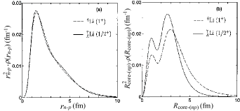
Figure 21: (a) the $n-p$ relative density of ${}^{7}_{\Lambda}{\rm Li}$ as a function of $r_{n-p}$ and (b) the $(np)$ c.m. density as a function of $R_{{\rm core}-(np)}$ together with the corresponding densities in ⁶Li core. This figure is taken from Hiyama99 .

We show in Fig. 21 the $n-p$ relative density $\rho(r_{n-p})$ and the $np$ c.m. density $\rho(R_{{\rm core}-(np)})$ together with the corresponding densities in ⁶Li core. The $n-p$ relative density exhibits almost the same shape for the ground state of ⁶Li and that of ${}^{7}_{\Lambda}$Li; namely, the shrinkage of the $n-p$ distance due to the $\Lambda$ participation is negligibly small. On the other hand, the $n-p$ c.m. density distribution of ${}^{7}_{\Lambda}$Li is remarkably different from that of ⁶Li, showing a significant contraction along the ${\bf R}_{{\rm core}-(np)}$ coordinate due to the $\Lambda$ addition. In fact, the r.m.s. distance ${\bar{R}}_{{\rm core}-(np)}$ is estimated to be 2.94 fm for ${}^{7}_{\Lambda}{\rm Li}(1/2^{+})$ versus 3.85 fm for ${}^{6}{\rm Li}(1^{+})$.

Thus, we concluded that, by the addition of the $\Lambda$ particle to ${}^{6}{\rm Li}(1^{+})$, contraction of ${}^{7}_{\Lambda}$Li occurs between the c.m. of the $(np)$ pair and the core whereas the $n-p$ relative motion remains almost unchanged. In this type change in the wave function, the angle operator in $B(E2)$ does not significantly affect the magnitude of shrinkage. We predicted in Ref. Hiyama99 that the size of ${\bar{R}}_{{\rm core}-(np)}$ in ⁶Li will shrink by 25 % due to the participation of a $\Lambda$ particle. In a later calculation Hiyama01c based on more precise ⁴He$+n+p+\Lambda$ 4-body model, we predicted it to be 22 %.

The first observation of the hypernuclear $B(E2)$ strength was made in the KEK-E419 experiment for $B(E2;5/2^{+}\rightarrow 1/2^{+})$ in ${}^{7}_{\Lambda}$Li. The observed $B(E2)$ value was $3.6\pm 0.5^{+0.5}_{-0.4}$ $e^{2}$fm⁴ Tanida01 . From this, the shrinkage of ${\bar{R}}_{{\rm core}-(np)}$ was estimated to be by $19\pm 4$ %, which was consistent with our prediction. It is to be emphasized that this interesting finding was realized with the help of our precision few-body calculations.

Our prediction about shrinkage of the ${}^{13}_{\Lambda}{\rm C}$ states was given in Ref. Hiyama97 ; Hiyama00 though experiment on ${}^{13}_{\Lambda}{\rm C}$ is not yet performed.

IV.3 Prediction of spin-orbit splitting in hypernuclei

In this subsection, we briefly review that the present authors and collaborators Hiyama00 predicted the spin-orbit splittings in hypernuclei ${}^{9}_{\Lambda}{\rm Be}$ and ${}^{13}_{\Lambda}{\rm C}$ and that afterwards it was confirmed by experiments at BNL Akikawa02 ; Ajimura01 .

One of the characteristic phenomena in non-strange nuclear physics is that there is a strong $NN$ spin-orbit interaction which leads to magic number nuclei. How large is the $YN$ spin-orbit interaction in comparison with the $NN$ spin-orbit one? It is known, for instance, that the antisymmetric spin-orbit ($ALS$) interactions are qualitatively different between one-boson-exchange (OBE) models Rijken75 ; Rijken99 and quark models Morimatsu84 ; Fujiwara96 . As a typical difference, the quark models predict that the $ALS$ component of the $\Lambda N$ interaction is so strong as to substantially cancel the $LS$ one, while the OBE models have (much) smaller $ALS$ and various strength of $LS$.

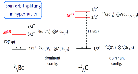
Figure 22: Successful GEM prediction of the spin-orbit splitting $\Delta E^{(LS)}$ in the hypernuclei ${}^{9}_{\Lambda}$Be and ${}^{13}_{\Lambda}$C (see Table 4).

Because of no $YN$ spin-polarized scattering data, however, we have no information on the strength of the interaction experimentally. Therefore, in order to extract information on it, careful calculations of hypernuclear structure should be of great help because $\Lambda$ spin-orbit splittings in hypernuclei are related straightforwardly to the spin-orbit component of $\Lambda N$ interactions.

In $\Lambda$-hypernuclei, spin-orbit splitting energy due to the $\Lambda N$ interaction was first precisely calculated in Ref. Hiyama00 (2000) for the $5/2^{+}_{1}-3/2^{+}_{1}$ doublet states in ${}^{9}_{\Lambda}{\rm Be}$ and the $3/2^{-}_{1}-1/2^{-}_{1}$ states in ${}^{13}_{\Lambda}{\rm C}$ (Fig. 22). The GEM calculation employed the $2\alpha+\Lambda$ model for ${}^{9}_{\Lambda}{\rm Be}$ and the $3\alpha+\Lambda$ model for ${}^{13}_{\Lambda}{\rm C}$  (Figs. 23 and  24). The total wavefunction was described as a sum of component functions corresponding those coordinate-channels in the figures, multiplied by the $\Lambda$-spin wavefunction.

We note that the core nuclei ⁸Be and ¹²C in these two hypernuclei are well described by the $2\alpha$- and $3\alpha$-cluster models, and that the spin-spin part of the $\Lambda N$ interaction vanishes and tensor term does not work in the $\Lambda\alpha$ folding potential. Therefore, calculation of the spin-orbit level splitting in ${}^{9}_{\Lambda}{\rm Be}$ and ${}^{13}_{\Lambda}{\rm C}$ using the folded $\Lambda\alpha$ spin-orbit potential will be useful to examine the qualitatively different two types of potential models, namely, OBE models Rijken75 ; Rijken99 and quark models Morimatsu84 ; Fujiwara96 mentioned above. The calculated spin-orbit splitting energies Hiyama00 are listed in Table 4.

Figure 23: Jacobi coordinates for the $2\alpha+\Lambda$ model of ${}^{9}_{\Lambda}$Be. The two $\alpha$ clusters are to be symmetrized.

Figure 24: Jacobi coordinates for the $3\alpha+\Lambda$ model of ${}^{13}_{\Lambda}$C. The three $\alpha$ clusters are to be symmetrized (totally 18-channels).

Afterwards, experimental values were reported as $\Delta E_{\rm EXP}(5/2^{+}_{1}{\rm-}3/2^{+}_{1})=31.4^{+2.5}_{-3.6}$ keV in ${}^{9}_{\Lambda}{\rm Be}$ by BNL-E930 Akikawa02 in 2002 and $\Delta E_{\rm CAL}(3/2^{-}_{1}{\rm-}1/2^{-}_{1})=150\pm 54\pm 36$ keV in ${}^{13}_{\Lambda}$C by BNL-E929 Ajimura01 in 2001, which is consistent with our prediction using the quark-based $\Lambda N$ spin-orbit force. The very weak spin-orbit component of the $\Lambda N$ interaction compared with that of the $NN$ interaction was confirmed.

Table 4: Spin-orbit splitting energies in ${}^{9}_{\Lambda}$Be and ${}^{13}_{\Lambda}$C. Calculated values by GEM are given in Ref. Hiyama00 using the OBE-model-based Rijken75 ; Rijken99 and quark-model-based Morimatsu84 ; Fujiwara96 $\Lambda N$ spin-orbit forces. Experimental values are taken from Akikawa02 for ${}^{9}_{\Lambda}$Be and from Ajimura01 for ${}^{13}_{\Lambda}$C. The theoretical prediction using the quark-based $\Lambda N$ spin-orbit force was confirmed by the experiments.

		CAL	CAL	EXP
		(OBE)	(quark)
	splitting	(keV)	(keV)	(keV)
${}^{9}_{\Lambda}$Be	$E(5/2^{+}_{1}{\rm-}3/2^{+}_{1})$	$80-200$	$35-40$	$31.4^{+2.5}_{-3.6}$
${}^{13}_{\Lambda}$C	$E(3/2^{-}_{1}{\rm-}1/2^{-}_{1})$	$390-960$	$\;150-200\;$	$150\pm 54\pm 36$

IV.4 Prediction for neutron-rich hypernuclei

It is of importance to produce neutron-rich $\Lambda$ hypernuclei for the fundamental study of hyperon-nucleon ($YN$) interaction. It is quite helpful to the newly developing experiments to predict energy levels of these $\Lambda$ hypernuclei before measurement.

In 2009, the present authors and collaborators Hiyama09He7L predicted energies of the ground and excited states of a neutron-rich hypernucleus ${}^{7}_{\Lambda}$He together with ${}^{7}_{\Lambda}{\rm Li}(T=1)$ and ${}^{7}_{\Lambda}{\rm Be}$ using an $\alpha+\Lambda+N+N$ 4-body cluster model. A part of the aim of this work was to help the new ${}^{7}{\rm Li}(e,e^{\prime}K^{+})^{7}_{\Lambda}{\rm He}$ experiment scheduled at JLAB.

We constructed 4-body Gaussian basis functions on all the Jacobi coordinates in Fig. 25 in order to take account of the full correlations among all the constituent particles. It is to be stressed that 2-body interactions among those particles were chosen so as to reproduce satisfactorily the observed low-energy properties of the subsystems ($NN$, $N\Lambda$, $N\alpha$, $\Lambda\alpha$, $NN\alpha$ and $N\Lambda\alpha$), at least all the existing binding energies of the subsystems Hiyama09He7L .

This condition for interactions is important in the analysis of the energy levels of these hypernuclei. Our analysis is performed systematically for both ground and excited states of $\alpha\Lambda NN$ systems with no more adjustable parameters in the stage of full 4-body calculation. Therefore, these predictions can offer an important guidance to the interpretation of upcoming hypernucleus experiments, ${}^{7}{\rm Li}(e,e^{\prime}K^{+})^{7}_{\Lambda}{\rm He}$ reaction at JLAB.

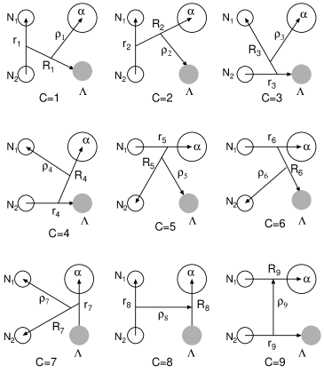
Figure 25: Jacobi coordinates for all the rearrangement channels ($c=1,...,9)$ of the $\alpha+\Lambda+N_{1}+N_{2}$ 4-body model for $\Lambda$-hypernuclei ${}^{7}_{\Lambda}{\rm He}$, ${}^{7}_{\Lambda}{\rm Li}$ and ${}^{7}_{\Lambda}{\rm Be}$ Hiyama09He7L . Two nucleons are to be antisymmetrized.

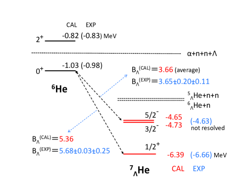
Figure 26: Calculated energy levels of ⁶He and ${}^{7}_{\Lambda}$He by Ref. Hiyama09He7L . The predicted $\Lambda$ binding energy $B_{\Lambda}^{({\rm CAL})}=3.66$ MeV for the excited states was afterwards reproduced by the experiment Gogami . This figure is taken from Ref. Hiyama09He7L .

As shown in Fig. 26, the $\Lambda$ binding (separation) energy $B_{\Lambda}$ of the $1/2^{+}$ ground state (namely, the binding energy measured from the ${}^{6}{\rm He(g.s.)}+\Lambda$ threshold) is calculated as $B_{\Lambda}^{\rm cal}=5.36$ MeV, while the $3/2^{+}$ and $5/2^{+}$ excited states are given at 1.66 and 1.74 MeV above the $1/2^{+}$ ground state, respectively.

In 2013, this hypernucleus ${}^{7}_{\Lambda}$He was observed by the JLAB E01-011 experiment with the ${}^{7}{\rm Li}(e,e^{\prime}K^{+})^{7}_{\Lambda}{\rm He}$ reaction and the $\Lambda$ separation energy was reported Nakamura13 as $B_{\Lambda}^{\rm exp}=5.68\pm 0.03({\rm stat.})\pm 0.25({\rm sys.})$ MeV, which is consistent with the theoretical prediction. Observation of the first excited-state peak ($3/2^{+}_{1}$ and $5/2^{+}_{1}$ unresolved) by the JLAB E01-015 experiment was reported Gogami with $B_{\Lambda}^{\rm exp}=3.65\pm 0.20({\rm stat.})\pm 0.11({\rm sys.})$ MeV, which agrees with the theoretical prediction $B_{\Lambda}^{\rm cal}=3.66$ MeV (average for the two excited states).

Those theoretical and experimental studies of the energies of ${}^{7}_{\Lambda}$He states are newly attracting strong attentions from the viewpoints of CSB (charge symmetry breaking) of the $YN$ interactions. For more details, see Ref. Hiya14He7L .

IV.5 Prediction of hypernuclear states with strangeness $S=-2$

Study of $\Lambda\Lambda$ interaction and $\Xi N$ interaction (both $S=-2$) is important. However, since hyperon-hyperon ($YY$) scattering experiment is difficult to perform, it is essential to extract information on these interactions from the structure study of $S=-2$ hypernuclei such as double $\Lambda$ hypernuclei and $\Xi$ hypernuclei.

For this aim, KEK-E373 emulsion experiment was performed and the ${}^{6}_{\Lambda\Lambda}$He was observed without ambiguity for the first time. The reported $\Lambda\Lambda$ binding energy (binding energy of ${}^{6}_{\Lambda\Lambda}$He measured from the ${}^{4}{\rm He(g.s.)}+\Lambda+\Lambda$ threshold) is $B_{\Lambda\Lambda}=6.91\pm 0.16$ MeV; analysis of the emulsion data to find new hypernuclei is still in progress. Besides, it is planned to perform, in 2017, new emulsion experiment at J-PARC (J-PARC-E07). However, since it is difficult to determine spins and parities of observed states, theoretical analysis is important for the identification of those states. The present authors and collaborators have succesfull experiences in interpreting the states of the following two double $\Lambda$ hypernuclei.

IV.5.1 Double $\Lambda$ hypernucleus ${}^{10}_{\Lambda\Lambda}$Be

The KEK-E373 experiment observed a double $\Lambda$ hypernucleus, ${}^{10}_{\Lambda\Lambda}$Be, which is called Demachi-Yanagi event Demachi-1 ; Demachi-2 ; Hida . The reported $\Lambda\Lambda$ binding energy was $B_{\Lambda\Lambda}^{\rm exp}=12.33_{-0.21}^{+0.35}$ MeV. However, it was not determined whether this event was observation of the ground state or any excited state in ${}^{10}_{\Lambda\Lambda}$Be.

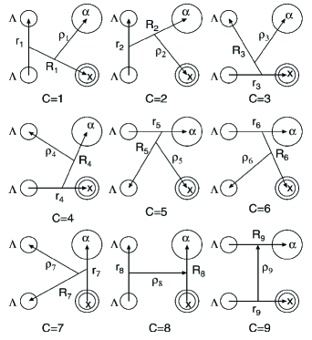
Figure 27: Jacobi coordinates for all the rearrangement channels ($c=1,...,9)$ of the $\alpha+X+\Lambda+\Lambda$ 4-body model. For the double $\Lambda$ hypernuclei ${}^{10}_{\Lambda\Lambda}$Be, we take $X=\alpha$. The two $\alpha$’s are to be symmetrized and the two $\Lambda$’s are to be antisymmetrized. Taken from Ref. Hiyama02doubleL .

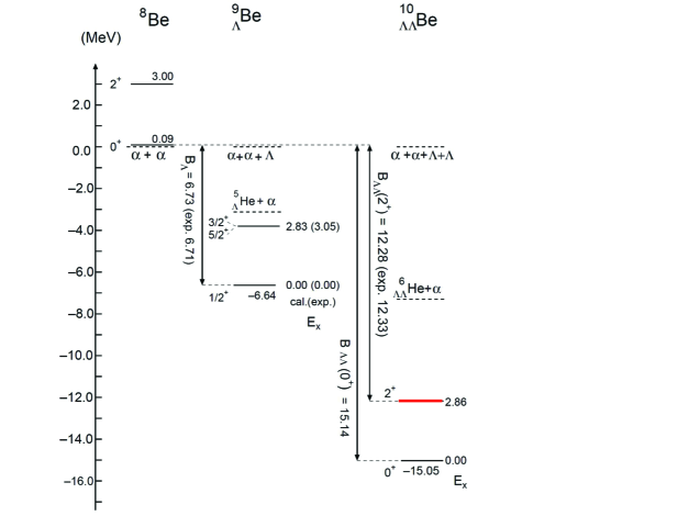
Figure 28: Calculated energy levels of ⁸Be, ${}^{9}_{\Lambda}$Be and ${}^{10}_{\Lambda\Lambda}$Be on the basis of the $\alpha\alpha$, $\alpha\alpha\Lambda$ and $\alpha\alpha\Lambda\Lambda$ models, respectively. The level energies are measured from the particle breakup thresholds or are given by excitation energies $E_{\rm x}$. This figure is taken from Ref. Hiyama02doubleL .

We studied ${}^{10}_{\Lambda\Lambda}$Be with the framework of $\alpha+\alpha+\Lambda+\Lambda$ 4-body model Hiyama02doubleL , constructing 4-body Gaussian basis functions on all the Jacobi coordinates in Fig. 27 in order to take account of the full correlations among all the constituent particles. Two-body interactions among those particles were chosen so as to reproduce satisfactorily the observed low-energy properties of the subsystems ($\alpha\Lambda$, $\alpha\alpha$ and $\alpha\Lambda\Lambda$, $\alpha\alpha\Lambda$). We then predicted, with no more adjustable parameters, the energy level of ${}^{10}_{\Lambda\Lambda}$Be.

As seen in Fig. 28, the calculated ${\Lambda\Lambda}$ binding energy of the $2^{+}$ state is $B_{\Lambda\Lambda}^{\rm cal}=12.28$ MeV, which is in good agreement with the experimental data. The Demachi-Yanagi event was then interpreted as the observation of the $2^{+}$ excited state of ${}^{10}_{\Lambda\Lambda}$Be (the ground state is located 2.86 MeV below). For more details, see Ref. Hiyama02doubleL in which more energy levels of ${}^{7}_{\Lambda\Lambda}$He, ${}^{7}_{\Lambda\Lambda}$Li, ${}^{8}_{\Lambda\Lambda}$Li, ${}^{9}_{\Lambda\Lambda}$Li and ${}^{9}_{\Lambda\Lambda}$Be are predicted though no experiment on them is done yet.

IV.5.2 Double $\Lambda$ hypernucleus ${}^{11}_{\Lambda\Lambda}$Be

The KEK-E373 experiment observed another new double $\Lambda$ hypernucleus, called Hida event Hida . This event had two possible interpretations: one is ${}^{11}_{\Lambda\Lambda}$Be with $B_{\Lambda\Lambda}=20.83\pm 1.27$ MeV, and the other is ${}^{12}_{\Lambda\Lambda}$Be with and $B_{\Lambda\Lambda}=22.48\pm 1.21$ MeV. It is uncertain whether this is observation of a ground state or an excited state.

Assuming this event to be ${}^{11}_{\Lambda\Lambda}$Be, we calculated the energy spectra of this hypernucleus within the framework of $\alpha+\alpha+n+\Lambda+\Lambda$ 5-body cluster model Hiyama10-Hida . All the interactions are tuned to reproduce the binding energies of possible subsystems (cf. Ref. Hiyama10-Hida for the details). There is no adjustable parameter when entering the 5-body calculation of ${}^{11}_{\Lambda\Lambda}$Be. The calculated $\Lambda\Lambda$ binding energy was $B_{\Lambda\Lambda}=18.23$ MeV, which does not contradict the interpretation that the Hida event is observation of the ground state of ${}^{11}_{\Lambda\Lambda}$Be.

As for $\Xi^{-}$ hypernuclei, there are a few experimental data at present. Among them, the observed spectrum of the $(K^{-},K^{+})$ reaction on a ¹²C target seems to indicate that the $\Xi$-nucleus interactions are attractive with a depth of $\sim 14$ MeV when a Woods-Saxon shape is assumed. Taking this information into consideration, we performed $\alpha+n+n+\Xi^{-}$ and $\alpha+\alpha+n+\Xi^{-}$ four-body cluster-model calculations, and predicted bound states for these hypernuclei. It is expected to perform search experiments for these $\Xi^{-}$ hypernuclei at J-PARC in the future. For more details, see Ref. Hiyama10Suppl-2 .

IV.6 Strategy of studying hypernuclei and $YN$ and $YY$ interactions

In the previous Secs. IV.2 – IV.5, we have reviewed some of our GEM studies of hypernuclei and $YN$ and $YY$ interactions. Here, we emphasize that one can obtain useful information on the $YN$ and $YY$ interaction combining few-body calculations of the hypernuclear structure and the related spectroscopy experiments on the basis of the following strategy (cf. Fig. 29):

(i) Firstly, we begin with candidates of $YN$ and $YY$ interactions that are based on the meson theory and/or the constituent quark model.

(ii) We then utilize spectroscopy experiments of hypernuclei. Generally, the experiments do not directly give any information about the $YN$ and $YY$ interactions.

(iii) Using the interactions in (i), accurate calculations of hypernuclear structures are performed. The calculated results are compared with the experimental data.

(iv) On the basis of this comparison, improvements for the underlying interaction models are proposed.

Following this strategy, we have succeeded in extracting information on the $YN$ and $YY$ interactions proposed so far with the use of GEM. These efforts are summerized in review papers Hiyama09PPNP ; Hiyama10Suppl-1 ; Hiyama10Suppl-2 ; Hiyama12FEW ; Hiyama12PTEP on the physics of hypernuclei and $YN$ and $YY$ interactions.

Figure 29: Strategy for extracting information about $YN$ and $YY$ interactions from the study of the structure of light hypernuclei. Taken from Ref. Hiyama12PTEP .

V Extension of GEM

V.1 Few-body resonances with the Complex-scaling method

We extended GEM to the case of calculating the energy and width of few-body resonances, employing the complex scaling method (CSM) CSM-ref1 ; CSM-ref2 ; CSM-ref3 ; Ho ; Moiseyev whose applications to nuclear physics problems are reviewed, for example, in Refs. Aoyama2006 . We applied GEM+CSM to the study of i) possibility of narrow 4-neutron resonance Hiyama16CSM using real-range Gaussian basis functions, and ii) new broad $0^{+}_{3}$ resonance in ¹²C Ohtsubo2013 using complex-range Gaussian basis functions.

The resonance energy (its position and width) is obtained as a stable complex eigenvalue of the complex scaled Schrödinger equation:

$$[H(\theta)-E(\theta)]\Psi_{JM,TT_{z}}(\theta)=0\;,$$ (19)

where $H(\theta)$ is obtained by making the complex radial scaling with an angle $\theta$

$$r_{\rm c}\to r_{\rm c}\,e^{i\theta},\;R_{\rm c}\to R_{\rm c}\,e^{i\theta},\;{\rho}_{\rm c}\to\rho_{\rm c}\,e^{i\theta},\;\;$$ (20)

for example, in the case of 4-body system of Fig. 9. According to the ABC theorem CSM-ref1 ; CSM-ref2 , the eigenvalues of Eq. (19) may be separated into three groups:

i) The bound state poles, remain unchanged under the complex scaling transformation and remain on the negative real axis.

ii) The cuts, associated with discretized continuum states, are rotated downward making an angle of $2\theta$ with respect to the real axis.

iii) The resonant poles are independent of parameter $\theta$ and are isolated from the discretized non-resonant continuum spectrum lying along the $2\theta$-rotated line when the relation tan 2$\theta>-{\rm Im}(E_{\rm res})/{\rm Re}(E_{\rm res})$ is satisfied. The resonance width is defined by $\Gamma=-2\,{\rm Im}(E_{\rm res})$.

V.1.1 Tetraneutron $(^{4}n)$ resonances

As a beautiful example that satisfies the above properties i)-iii), we show, in Fig. 30, narrow and broad resonances as well as the non-resonant continuum spectrum of the 4-neutron system (tetraneutron, ${}^{4}n$) Hiyama16CSM ; they are rotated in the complex energy plane from $\theta=10^{\circ}-22^{\circ}$.

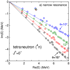
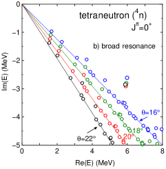
Figure 30: Dependence of the eigenenergy distribution on the complex scaling angle $\theta$ for the ${}^{4}n$ system with $J^{\pi}=0^{+}$. Two different cases are considered a) presence of a narrow resonance at $E_{\rm res}=3.65-0.66i$ MeV for $W_{1}(T=3/2)=-28$ MeV and b) presence of a broad resonance at $E_{\rm res}=5.88-2.85i$ MeV for $W_{1}(T=3/2)=-21$ MeV. Taken from Ref. Hiyama16CSM .

In Ref. Hiyama16CSM , we discussed about the theoretical possibility to generate a narrow resonance in the 4-neutron system as suggested by a recent experimental result ($E_{\rm res}=0.83\pm 0.65\pm 1.25$ MeV and $\Gamma\leq 2.6$ MeV) Kisamori-PRL . This experiment provides a good chance to investigate the isospin $T=3/2$ component of the 3-nucleon ($3N$) force since the $T=1/2$ component does not work in this system; the $T=3/2$ component has been considered to be smaller than the $T=1/2$ one in the literature.

To investigate this problem, we introduced a phenomenological $3N$ force for $T=3/2$ (in the same functional form of the $T=1/2$ one; cf. Eq. (2.2) of Ref. Hiyama16CSM ) in addition to a realistic $NN$ interaction (AV8^′). We inquired what should be the strength of the $T=3/2$ $3N$ force (compare with the $T=1/2$ one) in order to generate such a resonance; we performed this by changing the strength parameter $W_{1}(T\!=\!3/2)$ of the $T=3/2$ $3N$ force. As for the $T=1/2$ $3N$ force, $W_{1}(T\!=\!1/2)=-2.04$ MeV is known from our study of the ground and second $0^{+}$ states of ⁴He (cf. Sec. III.3).

The reliability of the $3N$ force in the $T=3/2$ channel was examined by analyzing its consistency with the low-lying $T=1$ states of ⁴H, ⁴He and ⁴Li and the ${}^{3}{\rm H}+n$ scattering. The ab initio solution of the $4n$ Schrödinger equation was obtained using the complex scaling method with boundary conditions appropriate to the 4-body resonances. We found that, in order to generate narrow $4n$ resonant states, unrealistically strong attractive $3N$ force is required as is explained below.

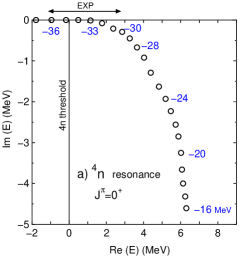
Figure 31: Tetraneutron (⁴n) resonance trajectory for the $J^{\pi}=0^{+}$ state. The circles correspond to resonance positions calculated in Ref. Hiyama16CSM . The strength parameter of the $T=3/2$ $3N$ force, $W_{1}(T=3/2)$, is changed from $-37$ to $-16$ MeV in steps of 1 MeV. To guide the eye, the resonance region suggested by the measurement Kisamori-PRL is indicated by the arrow at the top. Very strong attructive force of $W_{1}(T=3/2)=-36$ to $-30$ is required to generate a resonance in the energy region. Taken from Ref. Hiyama16CSM .

In Fig. 31, we display the trajectory of the ${}^{4}n$ S-matrix pole (resonance) with $J=0^{+}$ state by reducing the $3N$-force strength parameter from $W_{1}(T\!=\!3/2)=-37$ to $-16$ MeV in step of $1$ MeV. We were unable to continue the resonance trajectory beyond $W_{1}(T=3/2)=-16$ MeV with the CSM, the resonance becoming too broad to be separated from the non-resonant continuum. To guide the eye, at the top of the same figure, we present an arrow to indicate the ${}^{4}n$ energy range ($E_{\rm res}=0.83\pm 0.65\pm 1.25$ MeV) suggested by the recent measurement Kisamori-PRL . In order to generate a ${}^{4}n$ resonance in our calculation, we need the strength of the $3N$ force in the $T=3/2$ channel so large as $W_{1}(T\!=\!3/2)=-36\>{\rm to}\>-30$ MeV.

In Ref. Hiyama16CSM , showing many reasons, we concluded that we find no physical justification for the issue that the $T=3/2$ term should be one order of magnitude more attractive than the $T=1/2$ one, as is required to generate tetraneutron states compatible with the ones claimed in the recent experimental data Kisamori-PRL . We therefore requested the authors of the experiment paper to re-examine their result. They say that additional experiment has been performed and analysis is under way.

V.1.2 3-body resonances in ¹²C studied with complex-range Gaussians

Use of the complex-range Gaussian basis functions, introduced in Sec. II.4, is powerful in CSM calculations since the CSM resonace wave function becomes very oscillatory when the rotation angle $\theta$ becomes large (though the wave function is still $L^{2}$ integrable).

In Sec. V.1.2, we show a typical example in order to demonstrate that the use of the complex-range Gaussians gives rise to much more precise result than that of the real-range Gaussians. In Ref. Ohtsubo2013 the present authors and collaborators studied the $3\alpha$-cluster resonances performing the 3-body GEM calculation with the complex-range Gaussian basis functions in the $3\alpha$ OCM (orthogonality condition model). The main purpose of the work was to discuss about the newly observed broad $0^{+}_{3}$ resonance, but here we do not enter it. Instead, we show a comparison of the two results by the use of two different types of Gaussian basis functions; both calculations took the same $3\alpha$-cluster model and the same interactions.

Figure 32 illustrates the $0^{+}$ eigenvalue distribution of the complex scaled Hamiltonian $H(\theta)$ for the $3\alpha$-cluster OCM model obtained by Kurokawa and Katō Kurokawa (2005) using the real-range Gaussian basis functions. The scaling angle is $\theta=16^{\circ}$. On the other hand, Fig. 33 by our calculation Ohtsubo2013 (2013) shows the same quantity as in Fig. 32, but using the complex-range Gaussian basis functions for $\theta=16^{\circ}$ (black) and $26^{\circ}$ (blue).

One sees that Fig. 33 gave much more precise result than that in Fig. 32; especially, the non-resonant continuum spectra are almost on straight lines even at $\theta=26^{\circ}$.

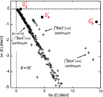
Figure 32: The $0^{+}$ eigenvalue distribution of the complex scaled Hamiltonian for the $3\alpha$ cluster OCM model obtained by Kurokawa and Katō Kurokawa using the real-range Gaussian basis functions. The scaling angle is $\theta=16^{\circ}$. This figure is to be compared with Fig. 33. Taken from Ref. Kurokawa .

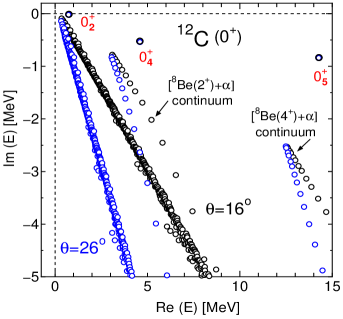
Figure 33: The $0^{+}$ eigenvalue distribution of the complex scaled Hamiltonian for the $3\alpha$ cluster OCM model with the use of the complex-range Gaussian basis functions. The scaling angles are $\theta=16^{\circ}$ (black) and $26^{\circ}$ (blue). This figure is to be compared with Fig. 32. Taken from Ref. Ohtsubo2013 .

In order to investigate the new broad $0^{+}_{3}$ resonance that was predicted in Ref. Kurokawa , we performed the CSM calculation for scaling angles from $\theta=22^{\circ}$ up to $36^{\circ}$. These large angles are required to reveal explicitly such a low-lying broad resonance separated from the 3-body continuum spectra. In our calculation Ohtsubo2013 , it was really possible to have the $0^{+}_{3}$ state at $E_{\rm res}=0.79-i\,0.84$ MeV as a clearly isolated and stable resonance pole against so large $\theta$ as $30^{\circ}-36^{\circ}$ (cf. Fig. 7 of Ref. Ohtsubo2013 ). See the paper for more about the $0^{+}_{3}$ state.

V.2 Few-body reactions with the Kohn-type variational principle to $S$-matrix

GEM is applicable to few-body reactions. In Sec. V.2, we review briefly three examples:

i) Muon transfer reaction in the cycle of muon catalyzed

fusion ($\mu$CF) (cf. Sec. III.1),

ii) Catalyzed big-bang nucleosynthesis (CBBN) reactions

(for review, see Ref. Kusakabe-review and Sec. 9.2 of Ref. Iocco ).

iii) Scattering calculation of 5-quark $(uudd{\bar{s}})$ systems.

The subjects i) and ii) give good tests to 3-body reaction theories for elastic and transfer processes in the presence of strong 3-body distortions (virtual excitations) in the intermediate stage of reaction.

V.2.1 Muon transfer reaction in $\mu$CF cycle

In the $\mu$CF cycle (cf. Fig. 22 of Hiyama03 ), muons injected into the $D_{2}/T_{2}$ mixture form finally $(d\mu)_{1s}$ and $(t\mu)_{1s}$, and then $(d\mu)_{1s}$ is changed to $(t\mu)_{1s}$ by the muon transfer reaction due to the difference in their binding energies:

$$(d\mu)_{1s}+t\to d+(t\mu)_{1s}+48\,{\rm eV}.$$ (21)

Figure 34: Three Jacobi coordinates of the $d+t+\mu^{-}$ system.

This reaction (cf. Fig. 34) was extensively studied theoretically in 1980’s and 1990’s as an important doorway process to the $\mu$CF and also by the following reason: Calculation of the cross section of this reaction at $E_{\rm cm}=0.001-100$ eV has been a stringent benchmark test for the calculation methods of Coulomb 3-body reactions. Since the muon mass is 207 times the electron mass, fully non-adiabatic treatment is necessary. The GEM calculaion Kamimura88b ; Kino93a gave one of the most precise results so far (cf. a brief review in Sec. 8.1 of Ref. Hiyama03 ).

We consider the reaction (21) at incident c.m. energies $0.001-100$ eV which are much less than the excitation energy of the $n=2$ state of $(t\mu)$ and $(d\mu)$, $\sim~{}\!2$ keV. The formulation below follows Sec. 8.1 of Ref. Hiyama03 :

The wave function which describes the transfer reaction (21) as well as the diagonal $(t\mu)_{1s}-d$ and $(d\mu)_{1s}-t$ processes with the total energy $E$ may be written as

$$\Psi_{JM}(E)=\phi^{(d\mu)}_{1s,\varepsilon_{1}}({\bf r}_{1})\,\chi^{(d\mu-t)}_{JM}(k_{1},{\bf R}_{1})$$

$$\qquad\quad\quad+\;\phi^{(t\mu)}_{1s,\varepsilon_{2}}({\bf r}_{2})\,\,\chi^{(t\mu-d)}_{JM}(k_{2},{\bf R}_{2})$$

$$\qquad\quad\quad+\;\sum_{\nu=1}^{\nu_{\rm max}}b_{\nu}(E)\Phi^{(\nu)}_{JM}(E_{\nu}).$$ (22)

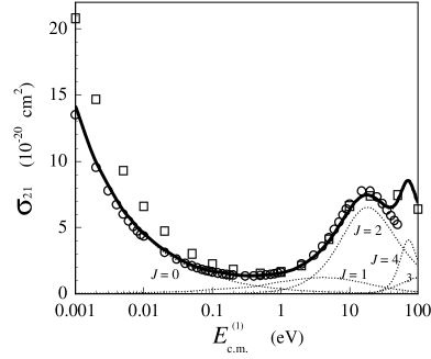
Figure 35: Calculated transfer cross sections $\sigma_{21}$ of $(d\mu)_{1s}+t\to d+(t\mu)_{1s}+48\ {\rm eV}$. $E_{\rm c.m.}^{(1)}=E-\varepsilon_{1s}^{(1)}$ is the collision c.m. energy in the incident channel. The results are given by GEM Kino93a (solid line), by Ref. Cohen91 (open boxes) and by Ref. Chiccoli92 (open circles). Dotted lines are partial-wave cross sections for each $J$ by GEM. Precise numbers of the cross sections are seen partially in Table 18 of Ref. Hiyama03 . This figure is taken from Ref. Hiyama03 .

The first and second terms describe the open channels $(d\mu)_{1s}-t$ and $(t\mu)_{1s}-d$, respectively. Here, $k_{1}$ is the wave number of the channel $c=1$ and is given as $\hbar^{2}k_{1}^{2}/(2\mu_{1})=E-\varepsilon_{1}$ with the intrinsic energy $\varepsilon_{1}$ ; and similarly for the channel $c=2$.

The third term is responsible, in the interaction region, for the 3-body degrees of freedom that are not included in the first and second terms. The third term is expanded by a set of $L^{2}$-integrable 3-body eigenfunctions (should nearly be a complete set in the restricted region). As such eigenfunctions, we employ $\{\Phi^{(\nu)}_{JM}(E_{\nu});\nu=1,...,\nu_{\rm max}\}$ with the eigenenergy $E_{\nu}$ that are obtained by diagonalizing the total Hamiltonian with the use of the 3-body Gaussian basis functions, Eqs. (3), whose total number is $\nu_{\rm max}$.

The authors of Refs. Kamimura88b ; Kino93a solved the unknown functions $\chi^{(d\mu-t)}_{JM}(k_{1},{\bf R}_{1})$ and $\chi^{(t\mu-d)}_{JM}(k_{2},{\bf R}_{2})$ as well as the unknown coefficients $\{b_{\nu}(E);\nu=1,...,\nu_{\rm max}\}$ by using the Kohn-type variational principle to $S$-matrix (see Sec. 4 of Ref. Kamimura77 for the general formulation and Secs. 2.5 and 8.1 of Ref. Hiyama03 ).

Figure 35 illustrates the calculated cross sections $\sigma_{21}$ of the reaction (21) by GEM Kino93a (solid line), by Ref. Cohen91 (open boxes) and by Ref. Chiccoli92 (open circles). As reviewed in Ref. Tolstikhin , the GEM calculations provides a standard result for the benchmark test calculations of this Coulomb 3-body reaction.

Here, we emphasize an important role of the third term of the total wave function (22); the term is responsible for the 3-body degrees of freedom in the interaction region. If we omit the term, the cross section $\sigma_{21}$ of the transfer reaction becomes more than ten times larger than $\sigma_{12}$ obtained above with the third term included.

Table 5: Summary of the calculated reaction rates of catalyzed big-bang nucleosynthesis (CBBN) reactions obtained by the 3-body GEM calculations Kamimura09 . The first three are for $T_{9}\lesssim 0.2$ and the others are for $T_{9}\lesssim 0.5$. Taken from Ref. Kamimura09 .

CBBN Reaction	Reaction rate (${\rm cm}^{3}\,{\rm s}^{-1}\,{\rm mol}^{-1}$) by GEM Kamimura09
non-resonant reaction
a) $(\alpha X^{-})+d\to~{}^{6}{\rm Li}+X^{-}$	$\quad 2.78\times 10^{8}\,T_{9}^{-\frac{2}{3}}\,{\rm exp}\,(-5.33\,T_{9}^{-\frac{1}{3}})(1-0.62\,T_{9}^{\frac{2}{3}}-0.29\,T_{9})$
b) $(\alpha X^{-})+t\to~{}^{7}{\rm Li}+X^{-}$	$\quad 1.4\times 10^{7}\,T_{9}^{-\frac{2}{3}}\,{\rm exp}\,(-6.08\,T_{9}^{-\frac{1}{3}})(1+1.3\,T_{9}^{\frac{2}{3}}+0.55\,T_{9})$
c) $(\alpha X^{-})+~\!\!{}^{3}{\rm He}\to~{}^{7}{\rm Be}+X^{-}$	$\quad 9.4\times 10^{7}\,T_{9}^{-\frac{2}{3}}\,{\rm exp}\,(-9.66\,T_{9}^{-\frac{1}{3}})\,(1+0.20\,T_{9}^{\frac{2}{3}}+0.05\,T_{9})$
d) $(^{6}{\rm Li}X^{-})+p\to~{}\alpha+~\!\!{}^{3}{\rm He}+X^{-}$	$\quad 2.6\times 10^{10}\,T_{9}^{-\frac{2}{3}}\,{\rm exp}\,(-6.74\,T_{9}^{-\frac{1}{3}})$
e) $(^{7}{\rm Li}X^{-})+p\to~{}\alpha+~{}\!\!\alpha+X^{-}$	$\quad 3.5\times 10^{8}\,\,T_{9}^{-\frac{2}{3}}\,{\rm exp}\,(-6.74\,T_{9}^{-\frac{1}{3}})\,(1+0.81\,T_{9}^{\frac{2}{3}}+0.30\,T_{9})$
f) $(^{7}{\rm Be}X^{-})+p\to~{}(^{8}{\rm B}X^{-})+\gamma$	$\quad 2.3\times 10^{5}\,T_{9}^{-\frac{2}{3}}\,{\rm exp}\,(-8.83\,T_{9}^{-\frac{1}{3}})\,(1+1.9\,T_{9}^{\frac{2}{3}}+0.54\,T_{9})$
resonant reaction
g) $(^{7}{\rm Be}X^{-})+p\to(^{8}{\rm B}X^{-})_{2p}^{\rm res.}$	$1.44\times 10^{6}\,T_{9}^{-\frac{3}{2}}\,{\rm exp}\,(-2.15T_{9}^{\,-1})\qquad m_{X}=100{\rm GeV}$
$\quad\>\to(^{8}{\rm B}X^{-})+\gamma$

This is due to the fact that, in such a low-energy reaction, the effect of the 3-body distortion (virtual excitation) induces a strong attractive force in the interaction region and causes severe mismatching of the wave length between the interaction region and the outside region, which results in the strong reduction of the transfer cross section.

V.2.2 Catalyzed big-bang nucleosynthesis (CBBN) reactions

The present authors and collaborators Hamaguchi ; Kamimura09 applied the 3-body reaction-calculation method in Sec. V.2.1 to the calculation of the reaction rates in the catalyzed big-bang nucleosynthesis (CBBN) reactions a) to g) in Table 5 and several more reactions (so-called rate-time CBBN reactions) in Table II of Ref. Kamimura09 . Those CBBN reaction rates were incoorpolated in the BBN network calculation in the literature and have been used for the study of the ⁶Li-⁷Li abundance problem, etc.

In the CBBN reactions a) to g), the particle $X^{-}$ stands for a hypothetical long-lived negatively-charged, massive ($\gtrsim 100$ GeV) leptonic particle such as a supersymmetric (SUSY) particle stau, a scalar partner of the tau lepton. It is known that if the $X^{-}$ particle has a lifetime of $\tau_{X}\gtrsim 10^{3}$ s, it would capture a light element previously synthesized in the standard BBN and forms a Coulombic bound state, for example, $(^{7}{\rm Be}X^{-})$ at temperature $T_{9}$ $\lesssim 0.4$ (in units of $10^{9}$ K), $(\alpha X^{-})$ at $T_{9}\lesssim 0.1$ and $(pX^{-})$ at $T_{9}\lesssim 0.01$. Those exotic-atom bound states are expected to induce the reactions a) to g) in which $X^{-}$ works as a catalysis.

Recent literature papers have claimed that some of these $X^{-}$-catalyzed reactions have significantly large cross sections so that inclusion of the reactions into the BBN network calculation can change drastically abundances of some elements; this can give not only a solution to the ⁶Li-⁷Li problem (calculated underproduction of ⁶Li by $\sim 1000$ times and overproduction of ⁷Li$+$⁷Be by $\sim 3$ times) but also a constraint on the lifetime and abundance of the elementary particle $X^{-}$.

However, most of these literature calculations of the reaction cross sections were made assuming too naive models or approximations that are not suitable for those complicated low-energy nuclear reactions. We performed a fully quantum three-body calculation of the cross sections of the above types of $X^{-}$-catalyzed reactions Hamaguchi ; Kamimura09 , and provided their reaction rates to the BBN network calculations. Our reaction rates are cited in recent review papers of BBN  Iocco and CBBN Kusakabe-review and have been actually used, for example, in Refs. Bailly2009CBBN ; Kusakabe-use ; Kubo-CBBN-use .

We note that GEM is responsible for such BBN network calculations using our CBBN reaction rates since absolute values of the cross sections were predicted (usually, such a prediction is difficult for nuclear reactions).

V.2.3 Scattering calculation of 5-quark $(uudd{\bar{s}})$ systems

In Ref. Hiyama06-penta , the present authors and collaborators performed a 5-body ($uudd{\bar{s}}$) scattering calculation, for the first time, about the penta-quark resonance $\Theta^{+}(1540)$ (experiment by Ref. penta ).

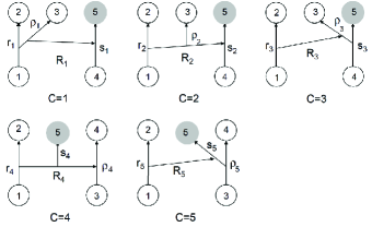
Figure 36: Five sets of Jacobi coordinates for the $uudd{\bar{s}}$ systems. Four $u,d$ quarks, labeled by particle $1-4$, are to be antisymmetrized, while particle 5 stands for ${\bar{s}}$ quark. Sets $c=4,5$ contain two $qq$ correlations, while sets $c=1-3$ do both $qq$ and $q{\bar{q}}$ correlations. Sets $c=1-3$ describe molecular configurations and sets $c=4,5$ does connected ones. The $NK$ scattering channel is treated with $c=1$. Taken from Ref. Hiyama06-penta

We took the five sets of Jacobi coordinates (Fig. 36) and employed the same framework of the previous Secs. V.2.1 and V.2.2. The $NK$ scattering channel is treated with $c=1$, described similarly as the first term of Eq. (22) (note that no second term in the present case). The channels $c=2-4$ stand for the 5-body degrees of freedom in the interaction region, described similarly as the third term of Eq. (22). We prepared a very large set of 5-body GEM basis functions and generated, by the bound-state approximation (diagonalization of the total Hamiltonian), the 5-body eigenstates $\{\Phi^{(\nu)}_{JM}(E_{\nu});\nu=1,...,\nu_{\rm max}\}$ with $\nu_{\rm max}\simeq 15,000$.

There is no bound state below the $NK$ threshold at $E=1.4$ GeV. Therefore, all the eigenstates $\Phi^{(\nu)}_{JM}(E_{\nu})$ are so-called pseudo-states, namely, discretized continuum states. It is not a priori known whether the pseudo-states become real resonances or non-resonant continuum states when the Schrödinger equation is fully solved under the $NK$-scattering boundary condition imposed.

Although a lot of pseudo-states $\Phi^{(\nu)}_{JM}(E_{\nu})$ with $J^{\pi}=\frac{1}{2}^{\pm}$ and $\frac{3}{2}^{\pm}$ were obtained within the bound-state approximation, all the pseeudo-states in $1.4-1.85$ GeV in mass around $\Theta^{+}(1540)$ melt into non-resonant continuum states when the coupling with the $NK$ scattering state is switched on (see the phase shifts in Fig. 37).

We then concluded, at the early stage of various discussions on $\Theta^{+}(1540)$, that there appears no 5-quark ($uudd{\bar{s}}$) resonance below 1.85 GeV in mass.

Figure 37: Calculated phase shifts for (a) $J^{\pi}=\frac{1}{2}^{-}$ and (b) $J^{\pi}=\frac{1}{2}^{+}$ states. The solid curves are given by the full-fledged calculation, while the dash-dotted curves are by the calculation with the elastic $NK$ channel alone. Energies are measured from the $NK$ threshold $(E_{\rm th})$. The arrow indicates the energy of $\Theta^{+}(1540)$ in $E-E_{\rm th}$. Taken from Ref. Hiyama06-penta .

VI Summary

We have reviewed our calculation method, Gaussian expansion method (GEM) Kamimura88 ; Kameyama89 ; Hiyama03 ; Hiyama12FEW ; Hiyama12PTEP for few-body systems, and its applications to various subjects. Those applications have been performed under our research strategy illustrated in Fig. 1. We studied few-body problems on

a) bound states using the Rayleigh-Ritz variational
       method,

b) resonant states using the complex-scaling method
       (Sec. V.1) and

c) reaction processes using the Kohn-type variational
       principle to $S$-matrix (Sec. V.2).

We have explained

 1) high accuracy of GEM calculations (Sec. III),

 2) successfull predictions by GEM calculations before
       measurements (Sec. IV) and

 3) wide applicability of GEM to few-body problems        in various reseach fields.

We introduced three types of Gaussian basis functions:

  i) real-range Gaussians (Sec. II.2),

 ii) complex-range Gaussians (Sec. II.4) and

iii) infinitesimally-shifted Gaussian lobe functions         (Sec. II.5).

All of the Gaussians have range parameters chosen to form geometric progression which is dense at short distances so that the description of the dynamics mediated by short-range interactions can be properly treated. Moreover approprite superposition of many Gaussians can decay accurately (exponentially) up to a sufficiently large distance (cf. Figs. 17 and 16 for a 4-body case).

The function space spanned by the basis functions of the second type ii) is much wider than that of the first type i), and is particularly good at describing highly oscillatory wave functions (cf. Figs. 45 and 46).

Use of the third type iii), mathematically equivalent to the first two, makes the calculation of few-body Hamiltonian matrix elements quite easier (with no tedius angular-momentum algebra) since the basis functions do not require any spherical harmonics function $Y_{lm}(\theta,\phi)$ to describe the angular part.

One of the advantages of taking the Gaussian ranges in geometric progression is that the number of variational parameters are so small that optimization of them can easily be performed. The GEM calculation is quite transparent in the sense that all the nonlinear variational parameters can be explicitly reported in a small table even in 4-body calculations (Sec. II.3).

The total wave function of bound (resonant) state is expanded in terms of few-body Gaussian basis functions of the Jacobi coordinates for all the rearrangement channels (Sec. II.1 for 3-body and Sec. III.3 for 4-body systems). This multi-channel representation makes the function space much wider than that spanned by single-channel basis functions. Therefore, those basis functions are particularly suitable for describing both the short-range behavior and long-range behavior (or weak binding) along any Jacobi coordinate of the system.

We are careful about all the pair interactions in order to reproduce the binding energies of all the subsystems. Therefore, there is no adjustable parameters when entering the full few-body calculation; the calculated result is ’predicted’ in this sense (Sec. IV).

We are interested in applying GEM to few-body problems in any fields that we have not enter yet (cf. Fig. 1 of our research strategy); collaboration for it is welcome.

APPENDIX

— Examples of accurate 2-body GEM calculations —

A.1 Harmonic oscillator potential

It is a good test to solve a problem whose exact analytical solution is known. We consider nucleon motion in a 3-dimensional harmonic oscillator (HO) potential:

$$\big{[}\,-\frac{\hbar^{2}}{2m_{N}}\nabla^{2}+\frac{1}{2}m_{N}\omega^{2}r^{2}-E\>\big{]}\,\phi_{lm}({\bf r})=0$$

with $\hbar^{2}/m_{N}=41.47$ MeV fm² and $\hbar\omega=15$ MeV. Radial part of the wave function is expanded in terms of the Gaussian basis functions of Eq. (5). The Hamiltonian and norm-overlap matrix elements can be calculated with Eqs. (12)-(15) in Ref. Hiyama03 . We take $l=0$.

Table 6: Test of the accuracy of GEM calculation for a nucleon in a harmonic oscillator potential with $\hbar\omega=15$ MeV using a set {$n_{\rm max}=10,\,r_{1}=1.5$ fm,  $r_{n_{\rm max}}=4.0$ fm} for $l=0$. The calculated and exact eigenenergies $(E^{(k)};k=1,...,7)$ are listed in terms of the number of quanta, $\varepsilon^{(k)}=E^{(k)}/{\hbar\omega}-3/2$.

k		$\varepsilon^{(k)}$ (GEM)		$\varepsilon^{(k)}$ (Exact)
1	$(0s)$	$0.000000$		$0\quad$
2	$(1s)$	$2.000000$		$2\quad$
3	$(2s)$	$4.000000$		$4\quad$
4	$(3s)$	$6.000005$		$6\quad$
5	$(4s)$	$8.000064$		$8\quad$
6	$(5s)$	$10.002508$		$10\quad$
7	$(6s)$	$12.015534$		$12\quad$

The Gaussian range parameters are chosen as {$n_{\rm max}=10$, $r_{1}=1.5$ fm, $r_{n_{\rm max}}=4.0$ fm} after a little try-and-error effort about $r_{1}$ and $r_{n_{\rm max}}$. More precise optimization is not necessary for practical use since the result is satisfactorily good as follows:

In Table LABEL:table:HO-energy, calculated energy $E^{(k)}$ of the $k$-th eigenstate $(k=1,...,7)$ is compared with the exact value; here $\varepsilon^{(k)}=E^{(k)}/{\hbar\omega}-3/2$ is presented. Wave function of the $5s\,(k=6)$ state is illustrated in Fig. 38. We obtain precise energies and wave functions for the lowest 6 states using 10 Gaussians. It can be said that the GEM well describes oscillating functions with 4 or 5 nodes (except for the origin); this will be enough in actual nuclear-potential problems.

As will be shown in Appendix A.6, use of the complex-range Gaussians can much more accurately describe, for example, the excited state with 19 oscillations in terms of 28 Gaussians for the same Schrödinger equation.

Figure 38: Wave function of a nucleon in a harmonic oscillator potential of $\hbar\omega=15$ MeV. The 5s state is illustrated. The solid line shows the GEM result using a set {$n_{\rm max}=10,\,r_{1}=1.5$ fm,  $r_{n_{\rm max}}=4.0$ fm}, while the closed circles denote the exact one.

A.2 Coulomb potential : hydrogen atom

Here, we consider the eigenstates of the hydrogen atom $(p+e^{-})$ as solution of the Schrödinger equation

$$\big{[}\,-\frac{1}{2}\nabla^{2}-\frac{1}{r}-E\>\big{]}\,\psi_{lm}({\bf r})=0\>,$$

where radius $r$ and energy $E$ are given in the atomic units of $\hbar^{2}/(m_{\rm e}e^{2})=0.5291$Å and $m_{e}e^{4}/\hbar^{2}=27.21$ eV.

Table 7: Calculated eigenenergies $E^{(k)}$ (in atomic unit) of the hydrogen atom with $l=0$ are compared with the exact values for the lowest 7 states. We took real-range Gaussians of {$n_{\rm max}=20$, $r_{1}=0.1$ a.u., $r_{n_{\rm max}}=80$ a.u.}.

k		$E^{(k)}$ (GEM)		$E^{(k)}$ (Exact)
1		$-0.499982$		$-0.500000$
2		$-0.124998$		$-0.125000$
3		$-0.055555$		$-0.055556$
4		$-0.031249$		$-0.031250$
5		$-0.019998$		$-0.020000$
6		$-0.013883$		$-0.013889$
7		$-0.010203$		$-0.010204$

In Table LABEL:table:Pe-energy, calculated eigenenergies $E^{(k)}(k=1,...,7)$ are compared with the exact values, $-1/(2k^{2})$, for $l=0$. We took the Gaussian range parameters as {$n_{\rm max}=20$, $r_{1}=0.1$ a.u., $r_{n_{\rm max}}=80$ a.u.}, which might be nearly the best set for $n_{\rm max}=20$; since $n_{\rm max}=20$ is sufficiently large for the lowest-lying 7 states, a little effort was necessary to optimize $r_{1}$ and $r_{n_{\rm max}}$ taking round numbers with the accuracy of 0.00001 a.u. in energy. Of course, we can obtain better solutions if we employ a larger basis set, but here we do not enter the problem. Much more accurate solution will be presented in Appendix A.6 with complex-range Gaussian basis functions.

A.3 Woods-Saxon potential

We solve $0s,1s$ and $0d$ bound states of neutron in a Woods-Saxon potential; namely, in the Schrödinger equation of Sec. A.1, we replace the H.O. potential by

$$V(r)=\frac{V_{0}}{1+{\rm e}^{(r-R_{0})/a}}$$

with $V_{0}=-55$ MeV, $R_{0}=3.0$ fm, $a=0.6$ fm and $\hbar^{2}/m=41.47$ MeV. The energy by the direct numerical calculation is listed in the first column of Table LABEL:table:WS-energy. Use of GEM calculation with a Gaussian basis set $\{n_{\rm max}=8,r_{1}=1.0\,{\rm fm},r_{n_{\rm max}}=6.0$ fm} gives the result in the second column of Table LABEL:table:WS-energy.

Table 8: Binding energies of the $0s$, $1s$ and $0d$ states of a neutron in the Woods-Saxon potential (see text) by the direct numerical calculation and the GEM calculations. The Gaussian basis set is $\{n_{\rm max}=8,r_{1}=1.0\,{\rm fm},r_{\rm max}=6.0\,{\rm fm}\}$.

		Exact		GEM
				($n_{\rm max}=8$)
$E_{0s}$ (MeV)		$-33.2531$		$-33.2528$
$E_{1s}$ (MeV)		$-3.2221$		$-3.2208$
$E_{0d}$ (MeV)		$-2.1897$		$-2.1893$

Figure 39: Wave functions of the $0s$, $1s$ and $0d$ states of a neutron in a Woods-Saxon potential (see text). The solid curve denotes the GEM result with eight Gaussians, whereas the dotted curve is the direct numerical one, but both curves are almost overlap in the whole region.

A satisfactorily accurate result is obtained by GEM. In Fig. 39, the wave functions given by the 8 Gaussian basis functions agree with those by the direct calculation.

A.4 Realistic $NN$ potential : deuteron

As a realistic $NN$ potential for solving deuteron, we employ the AV8^′ potential AV8P97 which is often used in few-body calculations such as the benchmark test calculation of ⁴He ground state Kamada01 which is mentioned in Sec. III C. The AV8^′ potential is expressed as a sum of central, spin-orbit and tensor forces; Fig. 40 shows its central part $(T=0,S=1)$ having a strong repulsive core and tensor part $(T=0)$.

Purpose of the GEM calculation of this system is to describe simultaneously both the strong short-range correlation and the asymptotic behavior accurately.

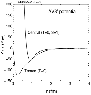
Figure 40: The AV8^′ $NN$ potential. The central part $(T=0,S=1)$ and tensor part $(T=0)$ are shown.

Figure 41: The $S$-wave and $D$-wave components of the deuteron wave function calculated by GEM with AV8^′.

We employ a Gaussian parameter set:
$\quad\{n_{\rm max}=15,\>r_{1}=0.2\,{\rm fm},\>r_{n_{\rm max}}=20\,$fm} for $S$-wave,
$\quad\{n_{\rm max}=20,\>r_{1}=0.2\,{\rm fm},\>r_{n_{\rm max}}=25\,$fm} for $D$-wave, namely, 35 basis functions totally.

Calculated wave function in the interaction region and that in the asymptotic region are illustrated respectively in Fig. 41 and Fig. 42. Strong reduction and steep increase of the wave-function magnitude due to the repulsive core is well derived. The correct asymptotic behavior (exponential decaying) of the wave function (multiplied by $r$) is demonstrated up to $r\sim 50$ fm where the amplitude is reduced by five-order of magnitude from the maximum value at $r\sim 1$ fm.

Figure 42: Asymptotic behavior of the deuteron $S$- and $D$-wave components (multiplied by $r$) by GEM with AV8^′.

A.5 Very strong short-range correlation and very long tail : ⁴He-atom dimer

To the authors’ knowledge, the most weakly bound 2-body state in nature is the ground state of ⁴He-atom dimer, and the most difficult problem to solve 2-body bound state with a central potential is this dimer state.

An example of the ⁴He-⁴He potential is the one called LM2M2 potential LM2M2 illustrated in Fig. 43 in red curve: this potential has a very strong repulsive core ($\sim\!10^{6}$ K at $r=0$) accompanied by shallow attractive tail ($\sim\!-10$ K pocket at $r=3$ Å) which results in a very weak bound state at $E=-0.00130$ K according to a precision direct numerical calculation by the step-by-step method. If we roughly scale this problem into a nuclear system, we would have a potential core height of $\sim 10^{6}$ MeV and an attractive pocket of $-10$ MeV at $r\sim 2$ fm, resulting in an extremely shallow bound state at $\sim-0.001$ MeV.

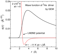
Figure 43: Wave function of the ⁴He-atom dimer (short-range region) calculated by GEM. The LM2M2 potential between ⁴He atoms is illustrated (in red curve) in arbitrary units. The only bound state is located at $E=-0.00130$ K, so shallow.

Figure 44: Wave function of the ⁴He-atom dimer (asymptotic region) calculated by GEM with the set $\{n_{\rm max}=60,\>r_{1}=0.25\,{\rm\AA},\>r_{n_{\rm max}}=700\,\AA\}$. The asymptotic behavior is correctly reproduced up to $\sim\!1000$ Å

.

Therefore, one might think that it would be almost impossible for any variational approach to solve this problem accurately, particularly the wave function having strong short-range correlations and a long-range asymptotic tail. But, it is possible to solve it using GEM. Diagonalization of Hamiltonian using our basis functions with the set $\{n_{\rm max}=60,\>r_{1}=0.25\,{\rm\AA},\>r_{n_{\rm max}}=700\,$ Å} gives the same energy ($E=-0.00130$ K) and wave function as those with direct numerical method; in Figs. 43 and 44 small difference between the results of the two method is not visible.

It is striking that both the short-range correlations and the exponentially-damped tail are simultaneously reproduced very accurately. This owes to the geometric-progression Gaussian ranges which have a dense distribution in the short-range region and a coherent superposition of long-range Gaussians in the asymptotic region. It will be difficult to reach this degree of agreement if other types of Gaussian-range set are chosen. This short-range correlations in the ⁴He dimer is relatively very much stronger than that in the realistic nucleon-nucleon interaction (AV8^′); notice the large difference in the degree of amplitude-attenuation in the short-range region in Fig. 43 for the ⁴He dimer and that in Fig. 41 for the deuteron $S$-wave.

In the cases of 3- and 4-body systems, the authors presented similar figures as Figs. 43 and 44 in Ref. Hiyama12COLD-1 (Figs. 3, 4, 6, 8, 10 and 11) and in Ref. Hiyama14COLD-3 (Figs. 4, 5, 8, 9 and 10) for ⁴He-atom clusters in the cold-atom physics.

A.6 Complex-range Gaussians basis functions

A.6.1. Highly excited states in HO potential

A good test of the use of complex-range Gaussian basis functions is to calculate the wave functions of highly excited states in a harmonic oscillator (HO) potential. We take the case of a nucleon with angular momentum $l=0$ in a potential having $\hbar\omega=15.0$ MeV. We expand the $s$-state wave function, $\Psi_{0}$, using Eq. (9) as

$$\Psi_{0}(r)=\sum_{n=1}^{n_{\rm max}}\big{[}c_{n}^{\rm(cos)}\phi^{\rm(cos)}_{n0}(r)+c_{n}^{\rm(sin)}\phi^{\rm(sin)}_{n0}(r)\big{]}.$$

Parameters of the complex-range Gaussians are $\{\,2n_{\rm max}=28,r_{1}=1.4\,{\rm fm},\,r_{n_{\rm max}}=5.8\,{\rm fm},\>\omega=\frac{\pi}{2}\frac{1}{1.2^{2}}=1.09\,\}$. For the sake of comparison, we also tested the real-range Gaussian basis functions with the parameters $\{n_{\rm max}=28,\>r_{1}=0.5\,{\rm fm},\>r_{n_{\rm max}}=11.3\,$fm}. Optimized $r_{1}$ and $r_{n_{\rm max}}$ are different between the two types of bases though their total numbers are the same. In Table 9, we compare the calculated energy eigenvalues with the exact ones. It is evident that the complex-range Gaussians can reproduce up to much more highly excited states than the real-range Gaussians do.

Table 9: Test of accuracy of real-range Gaussian and complex-range Gaussian basis functions for highly excited states with $l=0$ of a HO potential. The number of basis functions is 28 for both cases. Energies are listed in terms of the number of quanta, $E/\hbar\omega-\frac{3}{2}$. Reproduced from Ref. Hiyama03 .

	Exact	Real-range	Complex-range
	$\;0$	$0.0000$	$\>0.0000$
	$\;4$	$\>4.0000$	$\>4.0000$
	$\;8$	$\>8.0000$	$\>8.0000$
	12	12.0000	12.0000
	16	$16.002\;\,$	16.0000
	20	$20.01\;\;\;$	20.0000
	24	$24.1\;\;\;\;\;$	24.0001
	28	$29.5\;\;\;\;\;$	28.0003
	32	$37.3\;\;\;\;\;$	$32.002\;\,$
	38	$53.8\;\;\;\;\;$	$\;\;{\bf 38.003}\;$
	46	$91.6\;\;\;\;\;$	$46.3\;\;\;\;\;$

Figure 45: Wave function of the $l=0$, N=19 (38-quanta) state obtained by diagonalizing the HO-potential Hamiltonian using 28 complex-range Gaussian basis functions. It is compared with the exact wave function but the difference is invisible since the error is less than a few % everywhere. See text for the Gaussian parameters. Reproduced from Ref. Hiyama03 .

Figure 45 shows good accuracy of the wave function of 19-th excited state having 38 quanta. Error is within a few %, much smaller than the thickness of the line.

Owing to the advantage mentioned above, the complex-range Gaussian basis functions can be used to describe discretized continuum-energy states in various calculations (for example, cf. Refs. Matsumoto03PS ; Matsumoto03CDCC ).

A.6.2 Highly excited states of hydrogen atom

We explore another typical example in which the complex-range Gaussian basis functions reproduce highly oscillatory functions with high accuracy. Table 10 lists the calculated energy eigenvalues of the hydrogen atom with $l=0,n=1-40$ compared with the exact values. Parameters of the complex-range Gaussian basis functions are $\{\,2n_{\rm max}=160,r_{1}=0.015\,{\rm a.u.}\,,\,r_{n_{\rm max}}=2000\,{\rm a.u.},\>\omega=1.5\}$. The energy is reproduced within a relative error of $5\times 10^{-8}$ up to the state with $n=30$. The wave function of the state with $n=26$ is illustrated in Fig. 46, both for the exact solution and the calculated one. The relative error of the calculated wave function is $10^{-7}-10^{-5}$ up to $r=1500$ a.u..

Table 10: Calculated energy eigenvalues of the hydrogen atom with $l=0,n=1-40$ compared with the exact values. Parameters of the complex-range Gaussian basis functions are taken to be $\{\,2n_{\rm max}=160,\,r_{1}=0.015$ a.u.$,\,r_{n_{\rm max}}=2000\,$a.u., $\>\omega=1.5\,$}. This table is taken from Ref. Hiyama03 .

$n$	$E_{\rm cal}\;{\rm(a.u.)}$	$E_{\rm exact}\;{\rm(a.u.)}$	rel. error
1	-4.999999845$\times 10^{-1}$	-5.000000000$\times 10^{-1}$	3.1$\times 10^{-8}$
3	-5.555555494$\times 10^{-2}$	-5.555555556$\times 10^{-2}$	1.1$\times 10^{-8}$
10	-4.999999983$\times 10^{-3}$	-5.000000000$\times 10^{-3}$	3.5$\times 10^{-9}$
26	-7.396449686$\times 10^{-4}$	-7.396449704$\times 10^{-4}$	2.4$\times 10^{-9}$
30	-5.555555323$\times 10^{-4}$	-5.555555556$\times 10^{-4}$	4.2$\times 10^{-8}$
36	-3.856834714$\times 10^{-4}$	-3.858024691$\times 10^{-4}$	3.1$\times 10^{-4}$
40	-3.106429115$\times 10^{-4}$	-3.125000000$\times 10^{-4}$	5.9$\times 10^{-3}$

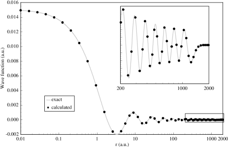
Figure 46: Wave function of the $l=0,\,n=26$ state of the hydrogen atom. The solid line is the exact one, and the dots are given by the complex-range Gaussian basis functions with the same parameters as in Table 2. Relative error of the latter is $10^{-7}-10^{-5}$ up to $r=1500$ a.u. at which absolute value of the wave function is four-order of magnitude smaller than that at $r=0$. This figure is taken from Ref. Hiyama03 .

References

- (1) M. Kamimura, Phys. Rev. A 38, 621 (1988).
- (2) H. Kameyama, M. Kamimura and Y. Fukushima, Phys. Rev. C 40, 974 (1989).
- (3) E. Hiyama, Y. Kino and M. Kamimura, Prog. Part. Nucl. Phys. 51, 223 (2003).
- (4) E. Hiyama, Few-Body Systems 53, 189 (2012).
- (5) E. Hiyama, Prog. Theor. Exp. Phys. 2012, 01A204 (2012).
- (6) Particle Data Group, D. E. Groom et al., Eur. Phys. J. C15, 1 (2000).
- (7) H.A. Torii et al., Phys. Rev. A 59, 223 (1999).
- (8) Y. Kino, M. Kamimura and H. Kudo, Nucl. Phys. A 631, 649c (1998).
- (9) Y. Kino, M. Kamimura and H. Kudo, Hyperfine Interact., 119, 201 (1999).
- (10) E. Hiyama, RCNP Physics Report (Research Center for Nuclear Physics, Osaka Univ.), RCNP-P-132 (1994), p.35.
- (11) E. Hiyama, Proceedings of International Workshop on the 4-Body Problems, Uppsala, 1995 (Uppsala Univ., 1996), p.28.
- (12) S. Aoyama, T. Myo, K. Kato, and K. Ikeda, Prog. Theor. Phys. 116, 1 (2006).
- (13) M. Kamimura, Prog. Theor. Phys. Suppl. 62 (1977) 236.
- (14) E. Hiyama and M. Kamimura, Phys. Rev. A 85, 022502 (2012).
- (15) E. Hiyama and M. Kamimura, Phys. Rev. A 85, 062505 (2012).
- (16) E. Hiyama and M. Kamimura, Phys. Rev. A 90, 052514 (2014).
- (17) S. Ohtsubo, Y. Fukushima, M. Kamimura, and E. Hiyama, Prog. Theor. Exp. Phys. 2013, 073D02 (2013).
- (18) T. Matsumoto, T. Kamizato, K. Ogata, Y. Iseri, E. Hiyama, M. Kamimura, and M. Yahiro, Phys. Rev. C 68, 064607 (2003).
- (19) T. Matsumoto, E. Hiyama, K. Ogata, Y.Iseri, M. Kamimura, S. Chiba, and M. Yahiro, Phys. Rev. C 70, 061601 (2003).
- (20) M. Kamimura, E. Hiyama, and Y. Kino, Prog. Theor. Phys. 121, 1059 (2009).
- (21) H. Preuss, Z. Naturforsch. 11a (1956) 823; J.L. Whitten, J. Chem. Phys. 39 (1963) 349; H. Sambe, J. Chem. Phys. 42 (1965) 1732; J.F. Harrison, J. Chem. Phys. 46 (1967) 1115; A.A. Frost, J. Chem. Phys. 47 (1967) 3707.
- (22) K. Nagamine and M. Kamimura, ”Muon catalyzed fusion: Interplay between nuclear and atomic physics”, Advance in Nuclear Physics, 24, 151 (1998)
- (23) V.I. Korobov, S.I. Vinitsky and I.V. Puzynin, Phys. Lett. B196 (1987) 272.
- (24) S.A. Alexander, H.J. Monkhorst, Phys. Rev. 38 26 (1988).
- (25) R.B. Wiringa, R.A. Smith and T.A. Ainsworth, Phys. Rev. C29 (1984) 1207.
- (26) M. Kamimura and H. Kameyama, Nucl. Phys. A 508 (1990) 17c.
- (27) S.A. Coon, M.D. Scardon, P.C. McName, B.R. Barrett, D.W.E. Blatt and B.H.J. McKeller, Nucl. Phys. A 317 (1979) 242.
- (28) C.R. Chen, G.L. Payne, J.L. Frier and B.F. Gibson, Phys. Rev. C31 (1985) 2266.
- (29) S. Ishikawa and T. Sasakawa, Few-Body Syst. 1 (1986) 143.
- (30) T. Sasakawa, in proceedings of the Workshop on Electron Nucleus Scattering, Elba International physics Center, Italy, 1988; Y. Wu, S. Ishikawa and T. Sasakawa, private communications (1989).
- (31) G.L. Payne and B.F. Gibson, Few-Body Syst. 14, 117, (1993).
- (32) H. Kamada, A. Nogga, W. Glöckle, E. Hiyama, M. Kamimura, K. Varga, Y. Suzuki, M. Viviani, A. Kievsky, S. Rosati, J. Carlson, S. C. Pieper, R. B. Wiringa, P. Navratil, B. R. Barrett, N. Barnea, W. Leidemann, and G. Orlandini, Phys. Rev. C 64, 044001 (2001).
- (33) B. S. Pudliner, V. R. Pandharipande, J. Carlson, S. C. Pieper, and R. B. Wiringa, Phys. Rev. C 56, 1720 (1997).
- (34) E. Hiyama, B.F. Gibson and M. Kamimura, Phys. Rev. C 70 031001(R) (2004).
- (35) W. Horiuchi and Y. Suzuki, Few-Body Systems 54, 2407 (2013).
- (36) Particle Data Group, C. Caso et al., Eur. Phys. J. C3 (1998) 1.
- (37) Y. Kino, M. Kamimura and H. Kudo, Few-Body Syst. Suppl. 12, 40 (2000).
- (38) Y. Kino, N.Yamanaka, M. Kamimura, P. Froelich and H. Kudo, Hyperfine Interactions, 138 (2001) 179.
- (39) E. Braaten and H.-W. Hammer, Physics Reports 428, 259 (2006).
- (40) R.A. Aziz and M.J. Slaman, J. Chem. Phys. 94, 8047 (1991).
- (41) R. Lazauskas and J. Carbonell, Phys. Rev. A 73, 062717 (2006).
- (42) M. Hori et al., Phys. Rev. Lett. 87, 093401 (2001).
- (43) Particle Data Group, K. Hagiwara et al., Phys. Rev. D 66, 010001 (2002).
- (44) T. Motoba, H. Bando and K. Ikeda,prog. Theor. Phys. 70, 189 (1983); T. Motoba, H. Bando, K. Ikeda and T. Yamada, Prog. Theor. Phys. Suppl. No. 81, 42 (1985).
- (45) E. Hiyama, M. Kamimura, K. Miyazaki, and T. Motoba, Phys. Rev. C 59, 2351 (1999).
- (46) E. Hiyama, M. Kamimura, T. Motoba, T. Yamada, and Y. Yamamoto, Phys. Rev. C 53, 2075 (1996).
- (47) E. Hiyama, M. Kamimura, T. Motoba, T. Yamada, and Y. Yamamoto, Nucl. Phys. A684, 227c (2001).
- (48) K. Tanida et al., Phys. Rev. Lett. 86, 1982 (2001).
- (49) E. Hiyama, M. Kamimura, T. Motoba, T. Yamada, and Y. Yamamoto, Prog. Theor. Phys. 97, 881 (1997).
- (50) E. Hiyama, M. Kamimura, T. Motoba, T. Yamada, and Y. Yamamoto, Phys. Rev. Lett. 85, 270 (2000).
- (51) H. Akikawa et al., Phys. Rev. Lett. 88, 82501 (2002).
- (52) S. Ajimura et al., Phys. Rev. Lett. 86, 4225 (2001).
- (53) M. M. Nagels, T. A. Rijken, and J. J. deSwart, Phys. Rev. D 12, 744 (1975); D 15, 2547 (1977); D 20, 1633 (1979).
- (54) T. A. Rijken, V. G. J. Stoks, and Y. Yamamoto, Phys. Rev. C 59, 21 (1999).
- (55) O. Morimatsu, S. Ohta, K. Shimizu, and K. Yazaki, Nucl. Phys. A 420, 573 (1984).
- (56) Y. Fujiwara, C. Nakamoto, and Y. Suzuki, Phys. Rev. Lett. 76, 2242 (1996).
- (57) E. Hiyama, Y. Yamamoto, T. Motoba and M. Kamimura, Phys. Rev. C 80, 054321 (2009)
- (58) S.N. Nakamura et al., Phys. Rev. Lett. 110, 012502 (2013).
- (59) T. Gogami, Ph.D thesis, Tohoku University, 2014.
- (60) E. Hiyama, M. Isaka, M. Kamimura, T. Myo, and T. Motoba, Phys. Rev. C 91, 054316 (2015).
- (61) J.K. Ahn et al., in Hadron and Nuclei, AIP Conf. Proc. No. 594, ed. II-Tong Cheon et al. (AIP, Meville, NY, 2001), p. 180.
- (62) A. Ichikawa, Ph.D. thesis, Kyoto University, 2001.
- (63) K. Nakazawa et al., Nucl. Phys. A 835, 207 (2010) (The proceedings on the 10th International Conference on Hypernuclear and Strange Particle Physics (Hyp X), Tokai, Sept.14-18, 2009); J.K. Ahn et al., Phys. Rev. C 88, 014003 (2013).
- (64) E. Hiyama, M. Kamimura, T. Motoba, T. Yamada and Y. Yamamoto, Phys. Rev. C 66, 024007 (2002)
- (65) E. Hiyama, M. Kamimura, Y. Yamamoto, and T. Motoba, Phys. Rev. Lett. 104, 212502 (2010).
- (66) E. Hiyama and T. Yamada, Prog. Part. Nucl. Phys. 63, 339 (2009).
- (67) E. Hiyama et al., Prog. Theor. Phys. Suppl. 185, 106 (2010).
- (68) E. Hiyama et al., Prog. Theor. Phys. Suppl. 185, 152 (2010).
- (69) J. Aguilar, and J.M. Combes, Commun. Math. Phys. 22, 269 (1971).
- (70) E. Balslev, and J.M. Combes, Commun. Math. Phys. 22, 280 (1971).
- (71) B. Simon, Commun. Math. Phys. 27, 1 (1972).
- (72) Y. K. Ho, Phys. Rep. 99, 1 (1983).
- (73) N. Moiseyev, Phys. Rep. 302, 211 (1998).
- (74) E. Hiyama, R. Lazauskas, Carbonell and M. Kamimura, Phys. Rev. C 93, 044004 (2016).
- (75) K. Kisamori et al., Phys. Rev. Lett. 116, 052501 (2016).
- (76) C. Kurokawa and K. Katō, Phys. Rev. C 71, 021301 (R) (2005).
- (77) M. Kusakabe, G.J. Mathews, T. Kajino, M.Ki. Cheoun, Int. J. of Mod. Phys. E, 26, 1741004 (2017).
- (78) F. Iocco et al., Phys. Reports 472, 1 (2009).
- (79) M. Kamimura, Muon Catalyzed Fusion 3, 335 (1988)
- (80) Y. Kino and M. Kamimura, Hyperfine Interactions, 82, 45 (1993).
- (81) J.S. Cohen and M.C. Struensee, Phys. A43, 3460 (1991).
- (82) C. Chiccoli, V.I. Korobov, V.S. Melezhik, P. Pasini, L.I. Ponomarev and J. Wozniak, Muon Catalized Fusion 7, 87 (1992).
- (83) O.I. Tolstikhin and C. Namba, Phys. Rev. A 60, 5111 (1999).
- (84) K. Hamguchi, T. Hatsuda, M. Kamimura, Y. Kino and T. Yanagida, Phys. Lett. B 650, 268 (2007).
- (85) M. Kubo, J. Sato, T. Shimomura, Y. Takanishi and M. Yamanaka, Phys. Rev. D 97, 115013 (2018).
- (86) M. Kusakabe, K.S. Kim, M.K. Cheoun, T. Kajino and Y. Kino Phys. Rev. D 88, 063514 (2013).
- (87) S. Bailly, K. Jedamzik and G. Moultaka, Phys. Rev. D 80, 063509 (2009).
- (88) E. Hiyama, M. Kamimura, A. Hosaka, H. Toki and M. Yahiro, Phys. Lett. B 633, 237 (2006).
- (89) LEPS Collaboration, T. Nakano et al., Phys. Rev. Lett. 91, 012002 (2003).