Star Clusters, Self-Interacting Dark Matter Halos and Black Hole Cusps:
The Fluid Conduction Model and its Extension to General Relativity

Abstract

We adopt the fluid conduction approximation to study the evolution of spherical star clusters and self-interacting dark matter (SIDM) halos. We also explore the formation and dynamical impact of density cusps that arise in both systems due to the presence of a massive, central black hole. The large N-body, self-gravitating systems we treat are “weakly-collisional”: the mean free time between star or SIDM particle collisions is much longer than their characteristic crossing (dynamical) time scale, but shorter than the system lifetime. The fluid conduction model reliably tracks the “gravothermal catastrophe” in star clusters and SIDM halos without black holes. For a star cluster with a massive, central black hole, this approximation reproduces the familiar Bahcall-Wolf quasistatic density cusp for the stars bound to the black hole and shows how the cusp halts the “gravothermal catastrophe” and causes the cluster to re-expand. An SIDM halo with an initial black hole central density spike that matches onto to an exterior NFW profile relaxes to a core-halo structure with a central density cusp determined by the velocity dependence of the SIDM interaction cross section. The success and relative simplicity of the fluid conduction approach in evolving such “weakly-collisional”, quasiequilibrium Newtonian systems motivates its extension to relativistic systems. We present a general relativistic extension here.

I Introduction

The fluid conduction approximation has been adopted successfully to study the dynamical evolution of a spherical star cluster, (see, e.g., Lynden-Bell and Eggleton (1980); Spitzer, Jr. (1987); Bettwieser and Sugimoto (1984); Bettwieser and Inagaki (1985); Goodman (1987); Heggie and Ramamani (1989); Balberg et al. (2002); Shapiro and Paschalidis (2014)) as well as a self-interacting dark matter (SIDM) halo (see, e.g.  Balberg et al. (2002); Ahn and Shapiro (2005); Shapiro and Paschalidis (2014)). In this approach the ensemble of gravitating particles is modeled by a “weakly-collisional” fluid in quasistatic, virial equilibrium. The local temperature is identified with the square of the velocity dispersion and thermal heat conduction is employed to reflect the manner in which orbital motion and scattering combine to transfer energy in the system. The basis of the heat conduction equations are moments of the Boltzmann equation, substituting a simple model for the collision terms.

This gravothermal fluid formalism was originally introduced for the study of globular star clusters, where it has proven to be very useful in understanding the secular evolution of these systems on relaxation timescales. The agreement between this fluid approach with more detailed (e.g, Fokker-Planck) treatments comes about despite the fact that star clusters are only weakly-collisional and have long collision mean free paths greatly exceeding the size of the cluster, where thermalization is achieved by the cumulative effect of repeated, distant, small-angle gravitational (Coulomb) encounters. The Fokker-Planck equation treats the phase space distribution function $f$, whose evolution is driven by diffusion coefficients involving integrals of $f$ over the entire system. By contrast, the fluid conduction equations evolve locally defined quantities (the density and velocity dispersion at a given spatial coordinate), although this approach incorporates a relaxation timescale and an effective mean free path in the heat conductivity that are based on global considerations and collision integrals over the entire system. In fact, the fluid conduction description may be even better suited to SIDM halos, for which the dominant thermalizing particle interactions in some models may be close-encounter, large-angle (hard-sphere) scatterings. It is reassuring, nevertheless, that, even in the case of weakly-collisional systems such as star clusters, the fluid conduction prescription does reproduce many of the results found in more fundamental analyses of the (weakly) collisional Boltzmann equation, with collisions treated via more precise, but computationally more demanding, Monte Carlo approaches or direct Fokker-Planck integrations (see reviews in, e.g.,  Spitzer, Jr. (1987); Lightman and Shapiro (1978); Shapiro (1985); Elson et al. (1987); Binney and Tremaine (1987), and a recent summary of methods in  Vasiliev (2015), and references therein). All of these approaches can be extended to treat anisotropic and multicomponent systems.

An isolated, self-gravitating N-body system in virial equilibrium will relax via gravitational encounters (scattering) to a state consisting of an extended halo surrounding a nearly homogeneous, isothermal central core. As time advances, the core transfers mass and energy through the flow of particles and heat to the extended halo. The thermal evolution timescale of the dense core is much shorter than that of the extended halo, which essentially serves as a quasistatic heat sink. As the core evolves it shrinks in size and mass, while its density and temperature grow. Increase of central temperature induces further heat transfer to the halo, leading to a secular instability on a thermal (collisional relaxation) timescale. The secular contraction of the core towards infinite density and temperature but zero mass is known as the “gravothermal catastrophe”(see, e.g., Spitzer, Jr. (1987)). The late-time, homologous nature of this secular instability is well-described by the fluid conduction model, as first shown by Lynden-Bell and Eggleton Lynden-Bell and Eggleton (1980). They solved the equations by separation of variables, looking for a self-similar solution applicable at late times.

A critical departure from the secular contraction scenario occurs when a dynamical instability sets in, which can occur when the particle velocities in the core, or, equivalently, when the central potential, become relativistic. As originally conjectured by Zel’dovich and Podurets Zel’dovich and Podurets (1966) and explicitly demonstrated by Shapiro and Teukolsky Shapiro and Teukolsky (1985a, b, 1986, 1992), collisionless systems in virial equilibrium typically experience a radial instability to collapse on dynamical timescales when their cores become sufficiently relativistic. This dynamically instability terminates the epoch of secular gravothermal contraction in clusters and leads to the catastrophic collapse of a core of finite mass to a black hole. The general relativistic simulations of the catastrophic collapse of relativistic clusters, which are essentially collisionless on dynamical timescales, by Shapiro and Teukolsky were performed in part to explore the possible origin of the supermassive black holes (SMBHs) that exist at the centers of most galaxies and quasars. Such a SMBH formation scenario might occur in relativistic clusters of compact stars following the gravothermal catastrophe Rees (1984); Shapiro and Teukolsky (1985c); Quinlan and Shapiro (1987, 1989). A similar SMBH formation scenario may also occur in SIDM halos, as originally proposed by Balberg and Shapiro Balberg and Shapiro (2002).

The existence of dense clusters of stellar-mass black holes and/or other compact objects in the cores of galaxies has been given a boost by the recent discovery of a swarm of black holes, inferred to be $2\times 10^{4}$ in number, within one parsec of the supermassive black hole Sagittarius A* at the center of the Galaxy Hailey et al. (2018). Concentrations ranging from several thousands to tens of thousands of stellar-mass black holes in this region have long been predicted by numerous investigators (see,e.g., Morris (1993); Miralda-Escudé and Gould (2000); Freitag et al. (2006); Generozov et al. (2018)). Such systems in the nuclei of other galaxies have been suggested (see, e.g., Elbert et al. (2018); Antonini and Rasio (2016) and references therein) as the likely sites for the formation of the binary black holes whose mergers have been observed by Advanced LIGO/VIRGO (e.g.,  Abbott et al. (2016, 2017)).

Here we briefly review the fluid conduction model and solve it numerically to evolve spherical, isotropic, single component star clusters and SIDM halos. To calibrate our code, we first integrate the full system of equations, starting from a Plummer model, to track the full evolution and development of the gravothermal catastrophe in star clusters. By contrast, the original treatment using this approach for isolated star clusters (see, e.g.,  Lynden-Bell and Eggleton (1980) and the summary in  Spitzer, Jr. (1987)) only considered the late-time, self-similar behavior, after the gravothermal catastrophe was well underway. We then apply the model to probe the effect of a massive, central black hole on the cluster density and velocity profiles, and its impact on the secular evolution of the system. While these features have been studied previously, they have not been analyzed by solving the fluid conduction equations. We recover the familiar Bahcall-Wolf ( Bahcall and Wolf (1976), hereafter BW) power-law profiles that dominate the central cusp embedded in a static, nearly homogeneous, isothermal core of equal-mass stars: the cusp density varies with radius as $\rho\propto r^{-7/4}$ and the velocity varies as $v\propto r^{-1/2}$. We then show how the presence of the cusp, which drives heat into core, eventually halts the gravothermal catastrophe, causing it to reverse its contraction and the cluster to re-expand. We predicted this behavior using a simple homologous cluster model Shapiro (1977) and it was corroborated subsequently by our Monte Carlo simulations of the two-dimensional Fokker-Planck equation for the stellar phase space distribution function $f(E,J;t)$ describing a spherical cluster containing a central black hole Marchant and Shapiro (1980); Duncan and Shapiro (1982) (see also Vasiliev (2017)).

In this paper we next apply the fluid conduction model to isolated SIDM halos, following up on our original treatment Balberg et al. (2002) of these systems. We previously explored the gravothermal catastrophe in such systems, probing both the late self-similar evolution of a typical system in which the mean free path between collisions $\lambda$ is initially longer than the scale height $H$ everywhere (which is always true in a star cluster), and then tracking the general time-dependent evolution of such systems. We found that $\lambda$ can eventually become smaller than $H$ in the innermost core, at which point that region behaves like a conventional fluid. At late times the core becomes relativistic and likely unstable to dynamical collapse to a black hole, as discussed above. We then determined the steady-state cusp that forms around a massive central black in an ambient, static SIDM core, solving the steady-state fluid conduction equations both in Newtonian gravity and general relativity Shapiro and Paschalidis (2014). We showed that the density in the cusp scales with radius as $r^{-\beta}$ for an interaction cross section that varies with velocity as $\sigma\sim v^{-a}$, where $\beta=(a+3)/4$.

By contrast, here we allow an SIDM halo to evolve in response to the central black hole. Specifically, we consider an SIDM halo born with a Navarro-Frenk-White (NFW) Navarro et al. (1997) density profile by the usual collisionless, cosmological halo formation mechanism. We assume that soon thereafter a central density spike forms in the halo in response to the adiabatic growth of a massive, central black hole. We then show, by solving the fluid conduction equations, that the spike evolves into a BW-like cusp which drives heat into the ambient halo, ultimately causing the core to expand, as in the case of a star cluster.

Given the utility of the fluid conduction model as demonstrated anew by the above applications, we present for the first time the full set of fluid conduction equations for following the secular evolution of a weakly-collisional system in general relativity. General relativistic simulations have been performed for the dynamical evolution of completely collisionless systems, as summarized above, as well as for relativistic fluid systems, such as stars. But as far as we are aware, there have been no implementations of a scheme to track the secular evolution of relativistic systems that are “weakly-collisional”. Yet as discussed above, the gravothermal catastrophe in star clusters and SIDM halos can ultimately drive Newtonian systems to a “weakly-collisional” relativistic state. The secular evolution of such a relativistic system immediately thereafter is governed neither by the collisionless Boltzmann (Vlasov) equation nor the “strongly-collisional” equations of relativistic hydrodynamics. It is thus necessary to provide a general relativistic formalism to bridge the epochs from Newtonian secular core contraction to relativistic dynamical collapse, and we do so here.

We emphasize that by focusing on the fluid conduction model in this paper we in no way offer it as a substitute for the more precise approaches mentioned above that have been designed, at least in Newtonian theory, to track the detailed evolution of weakly-collisional, large $N$-body, self-gravitating systems. Rather, our treatment here is presented to highlight the robustness and versatility of a scheme that is capable of physically reliable, first approximations to solutions of a great many problems that can be obtained with a minimum of computational resources and time. All calculations reported in this paper were performed on a single laptop. In the case of relativistic systems, we provide an approach where no schemes have been presented previously.

In Sec. II we present the Newtonian fluid conduction equations for spherical, isotropic systems and cast them into two different forms, both of which are useful numerically. In Sec. III we apply these equations to probe the secular evolution of several astrophysically realistic systems. These include a star cluster that begins as a Plummer model and undergoes the gravothermal catastrophe, as well as a Plummer model in which we suddenly insert a massive, central black hole and follow the resulting dynamical behavior. We also treat the secular evolution of SIDM halos containing a massive, central black hole. In Sec IV we present the general relativistic fluid conduction equations for spherical, isotropic systems.

We adopt geometrized units and set $G=1=c$ throughout.

II Newtonian Treatment

The basic Newtonian fluid conduction equations are given by Lynden-Bell and Eggleton (1980); Spitzer, Jr. (1987); Balberg et al. (2002); Shapiro and Paschalidis (2014)

$$\frac{\partial M}{\partial r}=4\pi r^{2}\rho$$ (1)

$$\frac{\partial(\rho v^{2})}{\partial r}=-\rho~{}\frac{M+M_{h}}{r^{2}}$$ (2)

$$\frac{\partial L}{\partial r} = -4\pi r^{2}\rho\left\{\frac{D}{Dt}\frac{3v^{2}}{2}+P\frac{D}{Dt}\frac{1}{\rho}\right\}$$ (3)

$$= -4\pi r^{2}\rho v^{2}\frac{D}{Dt}\ln\left(\frac{v^{3}}{\rho}\right)$$ (6)

Equation (2) is the equation of hydrostatic equilibrium, where $\rho$ is the matter density, $v$ is the one-dimensional matter velocity dispersion, $M=M(r)$ is the mass of matter interior to radius $r$, $M_{h}$ is the central black hole mass, if present, and $P$ is the the kinetic matter pressure, which satisfies $P=\rho v^{2}$. Equation  (3) is the the first law of thermodynamics for the rate of change of $\ln s$, the specific entropy of the matter, where we define $s$ by

$$s=\left(\frac{v^{3}}{\rho}\right).$$ (7)

The quantity $L$ is the luminosity due to heat conduction. The time derivatives in Eq. (3) are Lagrangian, and follow a given mass element.

For all applications considered in this paper $L$ is a conductive heat flux evaluated in the long mean free path limit,

$$\frac{L}{4\pi r^{2}}=-3b\rho\frac{H^{2}}{t_{r}}\frac{\partial v^{2}}{\partial r}.$$ (8)

(But see Balberg et al. (2002), Eq. 13 for the more general case). In writing Eq. (8) we evaluated the kinetic temperature of the particles according to $k_{B}T=mv^{2}$, where $k_{B}$ is Boltzmann’s constant. The parameter $b$ is constant of order unity and $H$ is the local particle scale height. The quantity $t_{r}$ is the local relaxation timescale. Its functional form depends on the matter interactions (Coulomb scattering for stars, other possibilities for SIDM) and will be assigned below for each application.

In the absence of a massive, central black hole the scale height is taken to be the local Jeans length $H=r_{J}=(3v^{2}/12\pi\rho)^{1/2}$ (see, e.g., Spitzer, Jr. (1987), Eq. 1-24) By contrast, in the presence of a black hole, the matter at $r$ that is bound to the black hole in the cusp and moves in a potential dominated by the hole has a scale height that is comparable to its characteristic orbital radius $r<<r_{J}$. For a system containing a black hole it proves sufficient then to set $H={\rm min}(r,r_{J})$, which accommodates the matter both inside and outside the cusp.

It is straightforward to generalize the set of equations to accommodate multicomponent systems containing particles of different masses and/or species. In such cases there will be separate hydrostatic equilibrium and entropy evolution equations for each component. In each entropy equation there will be, in addition to the self-interaction heat conduction term, pairwise thermal coupling terms to all the other components. These terms are each proportional to the difference in the local temperatures of the components and conduct heat from hotter to colder members (see, e.g.,  Bettwieser and Inagaki (1985)). The effect of these coupling terms is to drive the system to equipartition, which in turn leads to mass segregation. In this paper, however, we shall focus on single component systems.

It is sometimes computationally useful to express the evolution equations using $M=M(r)$ as the independent Lagrangian variable in order to maintain adequate coverage of the matter over the vast dynamical range of density and radius that accompanies the gravothermal instability or the formation of a cusp around a central black hole. Consequently we have $r=r(t,M)$, $\rho=\rho(t,M)$, etc, and Eqs. (1)-(8) become

$$\frac{\partial r}{\partial M}=\frac{1}{4\pi r^{2}\rho},$$ (9)

$$\frac{\partial(\rho v^{2})}{\partial M}=-\frac{M+M_{h}}{4\pi r^{4}}\rho,$$ (10)

$$\frac{L}{4\pi r^{2}}=-3b\rho\frac{H^{2}}{t_{r}}4\pi\rho r^{2}\frac{\partial v^{2}}{\partial M},$$ (11)

and

$$\frac{D}{Dt}\ln\left(\frac{v^{3}}{\rho}\right)=-\frac{1}{v^{2}}\frac{\partial L}{\partial M}.$$ (12)

The above system of equations for a virialized cluster is quite similar in form to the equations of stellar evolution, where one is also solving for the secular evolution of a configuration in hydrostatic equilibrium.

II.1 Star Clusters

II.1.1 Relaxation Timescale

In a star cluster relaxation is driven by multiple, small-angle gravitational (Coulomb) encounters. The local relaxation time scale is given by (see e.g., Lightman and Shapiro (1978); Spitzer, Jr. (1987))

$$t_{r}({\rm stars}) = \frac{3^{3/2}v^{3}}{4\pi\alpha m\rho\ln(0.4N)},$$ (13)

$$\simeq 0.7\times 10^{9}\mbox{yr}\left(\frac{v}{\mbox{km}~{}{\mbox{s}ec}^{-1}}\right)^{3}$$ (14)

$$\times \left(\frac{M_{\odot}{\mbox{pc}^{-3}}}{\rho}\right)\left(\frac{M_{\odot}}{m}\right)\left(\frac{1}{\ln(0.4N)}\right),$$ (15)

where $\alpha=1.22$, $m$ is the stellar mass and $N$ is the total number of stars in the cluster.

II.1.2 Nondimensional Equations

It is computationally convenient to cast the fluid conduction Eqs. (9)-(12) into nondimensional form. This is accomplished by introducing a fiducial mass $M_{0}$ and radius $R_{0}$, in terms of which corresponding nondimensional parameters are denoted by a tilde according to

$$r = R_{0}{\tilde{r}},$$ (16)

$$M = M_{0}{\tilde{M}}.$$ (17)

The parameters $M_{0}$ and $R_{0}$ then define a characteristic velocity, density, timescale, and entropy parameter,

$$v_{0} = \left(\frac{M_{0}}{R_{0}}\right)^{1/2},\;\;\;4\pi\rho_{0}=\left(\frac{M_{0}}{R_{0}^{3}}\right),$$ (18)

$$t_{0} = t_{r0}\frac{1}{6b}~{},\qquad\qquad\,s_{0}=\frac{v_{0}^{3}}{\rho_{0}}~{},$$ (19)

which yield corresponding nondimensional quantities,

$$v = v_{0}{\tilde{v}},\quad\rho=\rho_{0}{\tilde{\rho}_{0}}\quad t=t_{0}{\tilde{t}}\quad s=s_{0}{\tilde{s}}.$$ (20)

In Eq. (18) $t_{r0}$ is the relaxation timescale in Eq. (13), evaluated for $v=v_{0}$ and $\rho=\rho_{0}$. The parameter $b$ appearing in Eqs. (11) and  (18) is equal to $0.45$ for star clusters Spitzer, Jr. (1987). Inserting Eq. (11) into Eq. (12), writing Eqs. (9)-(12) in terms of nondimensional variables, and then dropping the tildes, yields

$$\frac{\partial r}{\partial M}=\frac{1}{r^{2}\rho}$$ (21)

$$\frac{\partial(\rho v^{2})}{\partial M}=-\frac{M+M_{h}}{r^{4}}\rho$$ (22)

$$\frac{D}{Dt}{\ln}~{}s=\frac{1}{v^{2}}\frac{\partial}{\partial M}\left[r^{4}\rho^{2}\left(\frac{H^{2}}{r_{J}^{2}}\right)\frac{\partial v}{\partial M}\right].$$ (23)

An alternative form for the entropy equation is

$$\frac{Ds}{Dt}=\frac{v}{\rho}\frac{\partial}{\partial M}\left[\frac{r^{4}\rho^{3}}{3v^{2}}\left(\frac{H^{2}}{r_{J}^{2}}\right)\frac{\partial s}{\partial M}+\frac{r^{4}\rho v}{3}\left(\frac{H^{2}}{r_{J}^{2}}\right)\frac{\partial\rho}{\partial M}\right].$$ (24)

The optimal way of numerically integrating the fluid conduction equations presumably would be to implement the Henyey method, as in a typical, battle-tested, stellar evolution code (see a description in, e.g., Clayton (1968), Sec 6-4). In the interest of obtaining quick results with minimal code writing or adaptation, it has proven adequate to integrate Eqs. (21)- (23) via a straightforward explicit forward-time, center-spaced finite-difference scheme. First, the diffusion-like (parabolic) evolution equation (23) is integrated forward in time on a timestep $\Delta t$ restricted by the (crudely estimated) Courant timestep:

$$\Delta t = 0.5~{}{\rm min}\left[\frac{(\Delta M)^{2}}{D}\right]\times C,$$ (25)

$$D \approx \frac{r^{4}\rho^{2}}{3v}\left(\frac{H^{2}}{r_{J}^{2}}\right),\ \ \ C\approx\mathcal{O}(1),$$ (27)

where $\Delta M$ is the grid spacing, $D$ is an effective diffusion constant, $C$ is a constant Courant factor of order unity, and the minimum is taken over all the grid points.

Next, using the value of $s(t,M)=v^{3}/\rho$ obtained at the new time, Eqs. (21) and  (22) are iterated to obtain $r(t,M),\rho(t,M)$ and $v(t,M)$ on that time. Solving Eq. (23) in a follow-up predictor-corrector step (or adopting a higher-order, time-centered, iterative scheme) is a refinement that was tested but proven unnecessary in practice for reliable results. The spatial differencing is second order in the Lagrangian variable $M$.

For clusters containing black holes, tracking the very late evolution and re-expansion proves difficult with the above explicit scheme, as the Courant timestep plummets when the cusp develops and the central (Lagrangian) grid spacing drops as the central density grows. Instead, we integrate Eq. (24) rather than Eq. (23), grouping the terms linear in $s$ and evaluating $s$ implicitly in time. Solving the resulting linear (tridiagonal) finite-difference equations for $s$ is no longer governed by a Courant condition for stability, so longer timesteps tuned to the evolution timescale, and not the decreasing conduction timescale across a central grid point, can be exploited (i.e. $C$ can be chosen much larger than unity). Once $s$ is determined on the new timestep, Eqs. (21) and  (22) may be iterated as before.

II.1.3 The Gravothermal Catastrophe

As our first application we track the secular evolution of a cluster that begins as a Plummer model without a central black hole (i.e. $M_{h}=0$).

Initial Data.

A Plummer model is an equilibrium polytrope of index $n=5$ that has a finite total mass $M_{P}$ and an infinite radius. We cut off the cluster at a finite radius containing 99% of the total mass. The Plummer density, velocity and mass profiles are given by (see, e.g.,  Spitzer, Jr. (1987), Eqs. (1-17)-(1-19))

$$\rho(r) = \frac{3M_{P}}{4\pi a^{3}}~{}\frac{1}{\left(1+r^{2}/a^{2}\right)^{5/2}}$$ (28)

$$v^{2}(r) = \frac{M_{P}}{a}~{}\frac{1}{6\left(1+r^{2}/a^{2}\right)^{1/2}}$$ (29)

$$M(r) = M_{P}~{}\frac{r^{3}/a^{3}}{\left(1+r^{2}/a^{2}\right)^{3/2}}$$ (30)

We use the total mass $M_{P}$ and the scale factor $a$ to set the mass and radius scale introduced in Eq. (16): $M_{0}\equiv M_{P}$ and $R_{0}\equiv a/2^{1/2}$.

Boundary Conditions

We assume regularity at the cluster center, e.g.,

$$\frac{\partial\rho}{\partial r}\to 0,\ \ \ \frac{\partial v}{\partial r}\to 0,\ \ \ \ M\to 0,$$ (31)

and take the density and pressure to vanish at the surface,

$$\rho=0,\ \ \ \rho v^{2}=0,\ \ \ M=1.$$ (32)

These conditions suffice to determine the system and are implemented in the finite difference equations. For example, Eqs. (31) and (32) are both used in finite differencing Eqs. (23) and  (24), while Eq. (32) is used in Eq. (22), starting at the cluster surface and integrating inward.

Numerical Results

The fluid conduction system of equations were finite-differenced with 281 grid points in $M$, logarithmically spaced. We set $H=r_{J}$ everywhere. The evolution equation for $s$ was integrated in time both explicitly via Eq. (23) and implicitly via Eq. (24). In both cases the timestep was set by Eq. (25) with $C$ equal to 3, although considerably higher values of $C$ also proved satisfactory using the implicit version, as expected. The two sets of integrations gave results that were very comparable; we will describe those obtained with the explicit implementation below. Integrations with half and twice as many grid points showed convergence with decreasing grid spacing.

The results of the numerical integration are summarized in Figs. 1– 3. The asymptotic behavior revealed in the plots at late times clearly exhibits the familiar gravothermal instability in a star cluster. Fig. 1 plots snapshots of the density profile at selected times and shows that the nearly homogeneous core undergoes contraction on a secular timescale, growing in central density while encompassing an ever decreasing fraction of the total mass. Once the contraction is well underway ($t\gg t_{rc}(0)$, where $t_{rc}(0)$ is the initial central relaxation timescale) the density approaches the self-similar solution of Lynden-Bell and Eggleton Lynden-Bell and Eggleton (1980) for gravothermal collapse. In particular, the density profile in the envelope approaches $\rho\propto r^{-(2+\beta)}\propto r^{-2.21}$, where $\beta=(1-\zeta)/(2-\zeta)$ and $\zeta=0.737$ (cf. Spitzer, Jr. (1987), Eqs. (3-33),(3-34)). Fig. 2 plots snapshots of the velocity dispersion profile at corresponding times, showing that the shrinking core is nearly isothermal, while the envelope dispersion scales as $v\sim(M(r)/r)^{1/2}\sim(\rho r^{2})^{1/2}\propto r^{-0.11}$. Fig. 3 illustrates good agreement with the asymptotic temporal relations that characterize the asymptotic self-similar solution (cf. Spitzer, Jr. (1987), Eqs. (3-6)–(3-8), (3-46) and (3-47)):

$$\frac{\rho_{c}}{\rho_{c}(0)} = \left[1-\frac{t}{t_{\rm coll}}\right]^{\frac{-2(5-3\zeta)}{(7-3\zeta)}}=\left[1-\frac{t}{t_{\rm coll}}\right]^{-1.165},$$ (33)

$$\frac{v_{c}}{v_{c}(0)} = \left[\frac{\rho_{c}}{\rho_{c}(0)}\right]^{\frac{(1-\zeta)}{2(5-3\zeta)}}=\left[1-\frac{t}{t_{\rm coll}}\right]^{-0.0550},$$ (36)

where $t_{\rm coll}$ is the core collapse time, at which the central density $\rho_{c}$ blows up to infinity while the core mass shrinks to zero. The velocity is thus seen to change much more slowly than the density during the collapse. We also recover asymptotically the self-similar solution result that the time remaining before complete collapse is a constant multiple of the instantaneous central relaxation time (cf. Spitzer, Jr. (1987), Eq. (3-47)),

$$\frac{t_{\rm coll}-t}{t_{rc}}=\frac{2(5-3\zeta)}{(7-3\zeta)}\frac{1}{\xi_{c}}\approx 320,$$ (37)

where $\xi_{c}\approx 3.6\times 10^{-3}$.

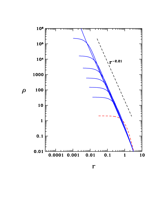
Figure 1: The gravothermal castastrophe: snapshots of the density profile at selected times. The curved dashed red line shows the density at time $t=0$. Successively higher solid blue curves show the density at $t=$ 2.107, 2.826, 3.159, 3.313, 3.378. 3.399, and 3.402. The straight dashed black line shows the slope for the self-similar solution, to which the envelope asymptotes at late times. All quantities are in nondimensional units defined in Eqs. (16–20), for which $t_{0}\approx 9.71t_{rc}(0)$.

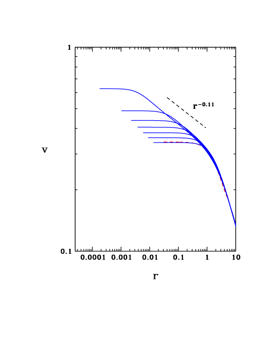
Figure 2: The gravothermal catastrophe: snapshots of the velocity dispersion profile at the same selected times depicted in Fig. 1. The core velocity dispersion increases with time. The straight dashed black curve shows the slope for the self-similar solution, to which the envelope asymptotes at late times. All quantities are in nondimensional units defined in Eqs. (16–20).

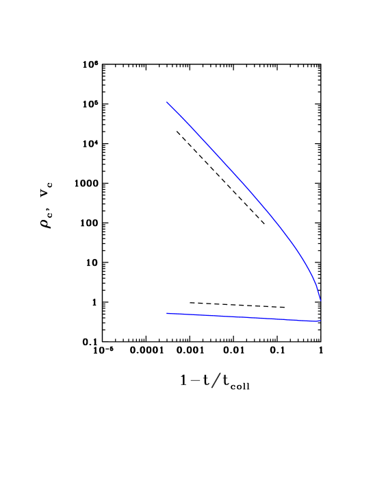
Figure 3: The gravothermal catastrophe: the central density (upper two lines) and velocity dispersion (lower two lines) as functions of time. The solid blue lines plot the results of integrating the full fluid conduction equations, while the dashed black lines show the late-time self-similar slopes, Eq. 33. The quantity $t_{\rm coll}$ is the core collapse time. All quantities are in nondimensional units defined in Eqs. (16–20)

II.1.4 Black Hole in a Static Ambient Cluster

Here we probe the formation of the cusp around a massive black hole $M_{h}<<M_{P}$ inserted at the center of the same Plummer star cluster described in Eq. (28). We fix for all $t\geq 0$ the cluster profile outside the inner core but allow the region near and within the black hole’s zone of influence at $r\leq r_{h}$ to relax in the presence of the hole. Here $r_{h}=M_{h}/v^{2}(0)$, where $v(0)$ is the central velocity dispersion in the initial cluster. The velocity dispersion is nearly constant in the core and remains unperturbed well outside $r_{h}$. We expect the cluster to evolve to the BW profile in the cusp and relax to a steady-state. Once again we take $M_{0}\equiv M_{P}$ and $R_{0}\equiv a/2^{1/2}$

Initial Data

We take $r_{h}/r_{\rm core}=10^{-3}$, where the core radius $r_{\rm core}$ is defined to be the radius at which the density $\rho$ falls to one-half its central value: $r_{core}=a(2^{2/5}-1)^{1/2}$ or $r_{core}=0.799$ in our nondimensional units. This choice of $r_{h}$ gives the black hole a mass $M_{h}/M_{P}=0.942\times 10^{-4}$, By construction, $M_{h}$ is much less than the total mass $M_{P}$ of the stars in the cluster, but much greater than the mass within the cusp ($r<r_{h}$), both initially and after steady-state is reached ($M(r_{h})/M_{h}=4.60\times 10^{-6}$ at late times). Accordingly, the gravitational potential of the black hole dominates that of the stars in the cusp. This is the regime modeled by BW. We take the same Plummer density profile given in Eq. (28) but we solve Eq. (10) for the initial velocity dispersion to ensure that the cluster with the central black hole is in virial equilibrium at the start of its secular evolution in the core. We neglect any initial contribution within $r_{h}$ from stars unbound to the black hole. They will generate a weak $r^{-1/2}$ cusp  Shapiro and Teukolsky (1983) that will be swamped by the cusp that forms from the bound stars as they begin to relax.

Boundary Conditions

An ordinary star of radius $R$ and mass $m$ is tidally disrupted by the black hole whenever it passes within a radius $r_{D}$, where

$$r_{D}\sim R(M_{h}/m)^{1/3}$$ (38)

However, sufficiently compact stars, such as neutron stars or stellar-mass black holes, may avoid tidal disruption before reaching the the marginally bound radius $r_{mb}$, where

$$r_{mb}=4M_{h}$$ (39)

in Schwarzschild coordinates. Even a main sequence star like the sun would escape disruption if the black hole exceeds $\sim 10^{8}M_{\odot}$. Any star that penetrates within $r_{mb}$ must plunge directly into the black hole (see, e.g, the discussion in Shapiro and Paschalidis (2014) and references therein). To mimic either scenario we fix a small inner radius $r_{in}$ within which the interior stellar mass is set to a vanishingly small value.

$$r=r_{in},\ \ \ M\to 0,$$ (40)

which implies $\rho=0$ for $r<r_{in}$. We put $r_{in}/r_{h}=3.81\times 10^{-2}$ to illustrate the effect.

The outer boundary $r_{out}$ is taken well outside the black hole radius of influence but well inside the core radius: $r_{out}=11.1r_{h}=1.11\times 10^{-2}r_{core}$. At $r_{out}$ we match all quantities to the Plummer model parameters, which are held fixed during the evolution:

$$r=r_{out},\ \ \,\rho=\rho_{P},\ \ \,\rho v^{2}=\rho_{P}v_{P}^{2},\ \ \ M=M(r_{out}).$$ (41)

With these assignments $M(r_{out})/M_{P}=2.51\times 10^{-7}$ and $M(r_{core})/M_{P}=0.119$.

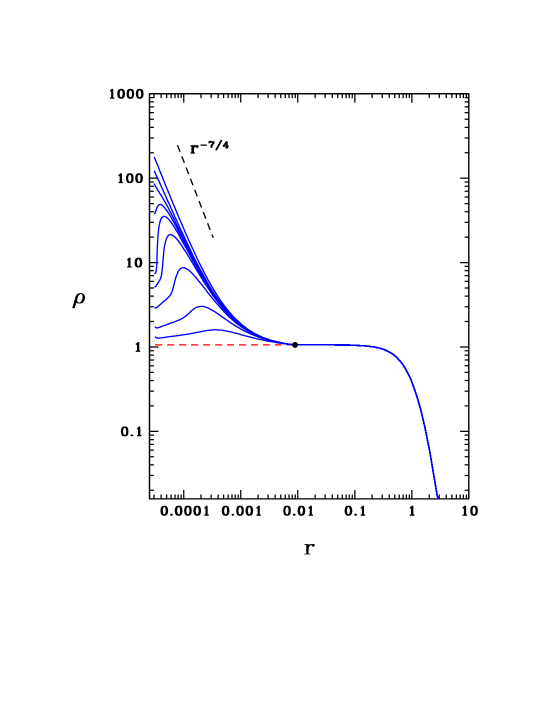
Figure 4: Black hole cusp in a static core: snapshots of the density profile at selected times. The lower dashed red line shows the density at time $t=0$. Successively higher solid blue curves show the density at $t=$ 0.0764, 0.1366, 0.1862, 0.2121, 0.2241, 0.2316, 0.2395, 0.2537, and 0.3330. The solid dot indicates the matching radius $r_{out}$, outside of which the profile is held fixed. The upper dashed black line shows the slope for the steady-state BW solution, to which the cusp relaxes. All quantities are in nondimensional units defined in Eqs. (16–20), for which $t_{0}\approx 9.71t_{rc}(0)$.

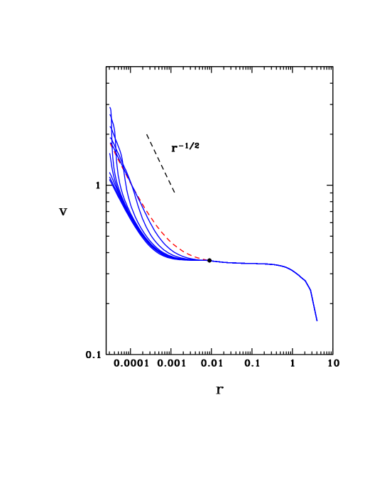
Figure 5: Black hole cusp in a static core: snapshots of the velocity dispersion profile at the same selected times depicted in Fig. 4. Successively lower solid curves are at increasing time. The solid dot indicates the matching radius $r_{out}$, outside of which the profile is held fixed. The straight dashed black curve shows the slope for the steady-state BW solution, to which the cusp relaxes. All quantities are in nondimensional units defined in Eqs. (16–20).

Numerical Results

The system of equations was integrated with 141 grid points covering the cluster, but with only 75 points inside $r_{out}$. The explicit form of the entropy evolution equation, Eq. (23), with Courant factor $C=1$ proved adequate. The evolution of the density and velocity profiles are shown in Figs. 4 and  5.

Relaxation drives the cusp to the familiar steady-state, power-law BW profile, as anticipated. Removing the constraint that the interior match to a fixed cluster core at $r_{out}$ will allow the cluster to evolve, as we will see in the next section. The BW solution for the cusp is readily seen as a consequence of the fluid conduction equations in steady state, in which case $L(r)=constant$ independent of $r$, according to Eq. (3). We used this result previously Shapiro and Lightman (1976) to derive the BW density profile from simple scaling. Now, by setting $\rho\propto r^{-\beta}$ and $M_{h}\gg M$ in Eq. (2) we obtain $v^{2}\approx[1/(\beta+1)]M_{h}/r$ inside the cusp. Requiring steady-state in Eq. (3 gives $L=constant$, which when inserted into Eq. (8) with $H\sim r$ yields $\beta=7/4$, as found by BW. The numerical integrations are in good agreement with these steady-state profiles.

II.1.5 Black Hole in an Evolving Cluster

Here we begin with the same cluster and central black hole as in Section II.1.4 above, but now we remove all constraints and allow the cluster to evolve. We are interested in observing the competition between those encounters that lead to the the gravothermal catastrophe and drive secular core collapse versus those arising from heating by the black hole cusp and drive core expansion.

Initial Data

We adopt the same initial data as in the previous section.

Boundary Conditions

We adopt the same black hole-induced inner boundary condition as in the previous section, Eq. (40). The outer boundary for such an isolated, freely-evolving cluster is set at the cluster surface via Eq. (32).

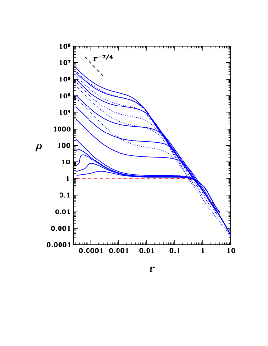
Figure 6: Black hole influence on cluster evolution: snapshots of the density profile at selected times. The lower dashed red line shows the density at time $t=0$. Successively higher solid blue curves show the density at $t=0.1286,0.1844,0.2163,0.2306,0.3447,5.954,9.611,10.98,11.44,\newline 11.48$ and $11.51$ (gravothermal collapse). Successively lower dotted blue curves then show the density at $t=11.53,11.81,14.36,23.11$ and $62.50$ (re-expansion). The upper dashed black line shows the slope for the steady-state BW cusp solution. All quantities are in nondimensional units defined in Eqs. (16–20), for which $t_{0}\approx 9.71t_{rc}(0)$.

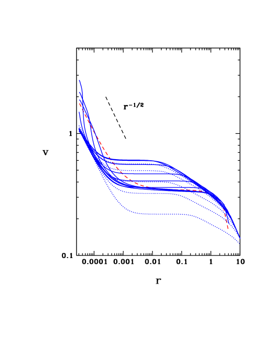
Figure 7: Black hole influence on cluster evolution: snapshots of the velocity dispersion profile at the same selected times depicted in Fig. 6. The straight dashed black curve shows the slope for the steady-state BW cusp solution, to which the cusp quickly relaxes. Once the dispersion velocity adjusts to the density cusp, the solid curves show successively higher core dispersions with increasing time (gravothermal collapse). The dotted curves then follow, showing successively lower core dispersions with increasing time (re-expansion). All quantities are in nondimensional units defined in Eqs. (16–20).

Numerical Results

We employ a grid of 141 points to integrate the system of equations, using the entropy evolution in the form given by Eq. (24) and solving it implicitly. A variable Courant constant $C$ was chosen for the timestep set by Eq. (25), increasing from $C=5$ at early times to $C=2\times 10^{12}$ at late times. The key reasons for the increase in $C$ are the huge growth in $\rho$ with time at the inner boundary of the cusp and the fact that $\Delta t$ as given by Eq. (25) plummets like $\rho^{-3}$ in this region.

The evolution of the cluster is summarized in Figs. 6 and  7. The early evolution in the cusp for $t\lesssim 0.23$ proceeds much as did in the previous application, where the ambient cluster was held fixed beyond the outer core. During this epoch the cusp, where the relaxation timescale is shortest, evolves in response to the presence of the black hole and again approaches a BW profile. But during an intermediate evolutionary phase when $0.23\lesssim t\lesssim 11.5$ the cluster interactions trigger incipient gravothermal core collapse. During this epoch the cusp maintains a BW profile with a density that smoothly matches onto the ever-increasing core density just outside $r_{h}$. The late evolution when $t\gtrsim 11.5$ is characterized by secular core re-expansion. Heating from the cusp drives the expansion, causing the core density and velocity disperion to fall and the outer mass shells to increase in radius. We predicted such expansion from a simple homologous cluster model in  Shapiro (1977) and probed its detailed nature by solving the Fokker-Planck equation by Monte Carlo simulations in  Marchant and Shapiro (1980); Duncan and Shapiro (1982) (see also Vasiliev (2017)). It is reassuring to see that the fluid conduction approach recovers the same qualitative behavior when a massive black hole resides at the center of a cluster.

II.2 Self-Interacting Dark Matter

We have applied the fluid conduction approximation to track the secular evolution of isolated SIDM halos in previous studies. Our initial application Balberg et al. (2002) treated the secular gravothermal catastrophe in Newtonian halos subject to elastic, velocity-independent interactions. There we showed that in typical halos $\lambda$, the mean free path for scattering, is much larger than the scale height $H$ initially, but once the contracting core evolves to sufficiently high density, the inequality is reversed in the innermost regions. This central region then behaves like a hydrodynamic fluid core surrounded by a weakly-collisional halo. We suggested Balberg and Shapiro (2002) that black hole formation is an inevitable consequence of the gravothermal catastrophe in SIDM halos once the core becomes sufficiently relativistic, as it becomes radially unstable and undergoes dynamical collapse. This scenario may produce the massive seed black holes that later merge and accrete gas to become the supermassive black holes observed in most galaxies and quasars.

We returned to the subject recently when we applied the fluid conduction approximation to model the steady-state distribution of matter around a massive black hole at the center of a weakly-collisional SIDM halo Shapiro and Paschalidis (2014). There we allowed the interactions to be governed by a velocity-dependent cross section $\sigma\sim v^{-a}$, solved the steady-state equations both in Newtonian theory and general relativity and showed that the SIDM density in the cusp scales as $\rho\sim r^{-\beta}$ away from the cusp boundaries, where $\beta=(a+3)/4$, while its velocity dispersion satisfies $v^{2}\approx[1/(\beta+1)]M_{h}/r$ or $v\sim r^{-1/2}$. For $a=4$ the interaction cross section has the same velocity dependence as Coulomb scattering and we recover the BW profile. In this case the solution we found applies to stars in a star cluster as well as SIDM. These steady-state calculations assumed that the ambient halo outside the cusp remained static, as we did in Section II.1.4 above for star clusters.

Missing from the above steady-state analysis is a time-dependent calculation that shows how the SIDM density and velocity profiles secularly evolve away from their initial configurations. Those initial configurations likely include a central density spike that arises early on, following the appearance and adiabatic growth of a central supermassive black hole on timescales shorter than the dark matter self-interaction relaxation time, $t_{r}(SIDM)$. The spike then evolves on the timescale $t_{r}(SIDM)$ into a weakly-collisional cusp and the entire halo then expands in response to the heat driven into the halo by the cusp. We shall perform a simulation that illustrates this behavior below.

II.2.1 Relaxation Timescale

In a SIDM halo relaxation is driven by elastic interactions between particles. The relaxation time scale is the mean time between single collisions and is given by

$$t_{r}({\rm SIDM}) = \frac{1}{\eta\rho v\sigma}$$ (42)

$$\simeq 0.8\times 10^{9}\mbox{yr}\left[\left(\frac{\eta}{2.26}\right)\left(\frac{\rho}{10^{-24}\mbox{g cm}^{-3}}\right)\right.$$ (43)

$$\times \left.\left(\frac{v_{*}}{10^{7}\mbox{cm sec}^{-1}}\right)\left(\frac{v}{v_{*}}\right)^{1-a}\left(\frac{\sigma_{0}}{1~{}\mbox{cm}^{2}\;\mbox{g}^{-1}}\right)\right]^{-1}\,$$ (44)

where $\sigma=\sigma_{0}(v/v_{*})^{-a}$ is the cross section per unit mass and the constant $\eta$ is of order unity. For example, $\eta=\sqrt{16/\pi}\approx 2.26$ for particles interacting elastically like billiard balls (hard spheres) with a Maxwell-Boltzmann velocity distribution [see Reif (1965), Eqs. (7.10.3), (12.2.9) and (12.2.13)]. We note again that for a Coulomb-like cross section, where $a=4$, $t_{r}({\rm SIDM})$ scales the same way with $v$ and $\rho$ as $t_{r}({\rm stars})$: $t_{r}\propto v^{3}/\rho$.

II.2.2 Nondimensional Equations

We modify the scalings for $\rho_{0}$ and $t_{0}$ defined in Eqs. (18) and (20) by choosing instead

$$\rho_{0}=\left(\frac{M_{0}}{R_{0}^{3}}\right),\;\;\;t_{0}=t_{r0}\frac{1}{6b}\frac{1}{4\pi},$$ (45)

while keeping the other scalings the same. Here $t_{r0}$ is given by Eq. (42), evaluated for $v=v_{0}$ and $\rho=\rho_{0}$. For a gas of hard spheres with a Maxwell-Boltzmann distribution the coefficient $b$ in Eq. (8) can be calculated to good precision from transport theory, and has the value of $b\approx(25/64)\sqrt{2\pi/3}\approx 0.565$ [cf. Lifshitz and Pitaevskii (1981), Sec. 10, Eq. (7.6) and Problem 3, and Spitzer, Jr. (1987), Eq. (3-35)]. For a gas obeying a Coulomb scattering cross section $b\approx 0.45$ Spitzer, Jr. (1987). The resulting nondimensional equilibrium Eqs. (21) and  (22) are unchanged but the entropy evolution Eq. (23) now becomes

$$\frac{D}{Dt}\ln s=\frac{1}{v^{2}}\frac{\partial}{\partial M}\left[r^{4}\rho^{2}v^{4-a}\left(\frac{H^{2}}{r_{J}^{2}}\right)\frac{\partial v}{\partial M}\right],$$ (46)

while Eq. (24) becomes

$$\frac{Ds}{Dt}=\frac{v}{\rho}\frac{\partial}{\partial M}\left[\frac{r^{4}\rho^{3}}{3v^{a-2}}\left(\frac{H^{2}}{r_{J}^{2}}\right)\frac{\partial s}{\partial M}+\frac{r^{4}\rho v^{5-a}}{3}\left(\frac{H^{2}}{r_{J}^{2}}\right)\frac{\partial\rho}{\partial M}\right].$$ (47)

The above equations apply to the long mean-free path (LMFP) limit that characterizes the early and longest secular evolution phase of an SIDM halo and the phase we wish to probe here. For the more general equations that handle the transition from the early LMFP phase to the late, short mean free path (SMFP) phase, when such a transition occurs, see  Balberg et al. (2002).

II.2.3 The Gravothermal Catastrophe

We previously treated in Ref Balberg et al. (2002) the evolution of a SIDM halo in the absence of a black hole and with a velocity-independent ($a=0$) interaction cross-section using the fluid conduction equations, and we will not repeat the analysis here. There we showed how a halo can evolve from the (self-similar) LMFP regime to the SMFP regime in the inner core of the halo and discussed how the catastrophic collapse of the core can naturally provide the seed for a supermassive black hole at the halo center. We discussed this SIDM-black hole formation scenario in greater detail in Ref Balberg and Shapiro (2002).

II.2.4 Black Hole in a Static Ambient Cluster

As mentioned in Sec. I, this scenario was treated in Ref Shapiro and Paschalidis (2014), both in Newtonian and general relativistic gravitation. We took $a=4$ for the velocity dependence in the SIDM interaction cross section in the example we worked out. We noted that any depletion in the DM density deep in the spike due to DM annihilation Gondolo and Silk (1999); Vasiliev (2007); Shapiro and Shelton (2016) would be washed out by self-interactions. We refer the reader to that paper for further details.

II.2.5 Black Hole in an Evolving Halo

Here we consider the full evolution of a SIDM halo, formed in the early Universe with an NFW profile, that houses a massive seed black hole at its center. We assume that the black hole grew adiabatically (e.g. by accretion) to supermassive size early on and that a SIDM central density spike formed in response the hole. We further assume that the appearance and adiabatic growth of the black hole took place on a timescale shorter than the SIDM relaxation timescale, Eq. (42), so that the density profile in the spike assumed a (power-law) form, appropriate for a collisionless spike responding to an adiabatically growing black hole in a power-law halo distribution  Gondolo and Silk (1999). We then simulate below how SIDM collisions drive the density spike to a weakly-collisional cusp around the hole and how heating from the cusp drives the subsequent expansion of the halo.

Initial Data

. Here we adopt a simplified halo profile that highlights the interior (cuspy) regions of an NFW halo containing a density spike around a central supermassive black hole. The density profile is given by

$$\rho(r) = 0,\ \ \ r\leq 4M_{h}\ \ ({\rm capture\ region}),$$

$$= \rho_{h}(r_{h}/r)^{\gamma_{sp}},\ \ \ \ \ \ 4M_{h}<r\leq r_{h}\ \ \ ({\rm spike}),$$

$$= \rho_{h}(r_{h}/r)^{\gamma_{c}},\ \ \ \ \ r_{h}<r\leq R_{H}\ \ \ ({\rm\ halo}).$$

Defining $M_{H}$ to be the total mass of the SIDM halo, $R_{H}$ the halo radius and $M_{h}$ the mass of the black hole, we set the scaling parameters $M_{0}=M_{H}$, $R_{0}=R_{H}/25$ and and $r_{h}=M_{h}/v_{0}^{2}$. We take $M_{h}/M_{H}=10^{-2}$, which gives $r_{h}/R_{H}=4\times 10^{-4}$. The density parameter $\rho_{h}$ is determined by substituting Eq. (II.2.5) into Eq. (1), integrating over the entire SIDM halo and setting the resulting mass equal to $M_{H}$. The velocity profile is determined by substituting Eq. (II.2.5) into Eq. (2) and integrating inward from the surface to find $v(r)$.

We choose $\gamma_{c}=1$, consistent with the standard NFW inner region profile. For a spike that forms about an adiabatically growing supermassive black hole we then require $\gamma_{sp}=(9-2\gamma_{c})/(4-\gamma_{c})$ Gondolo and Silk (1999), which yields $\gamma_{sp}=2.33$. We set $a=4$ in the velocity-dependent SIDM interaction cross section as we did in Ref Shapiro and Paschalidis (2014).

We note that with the adopted initial data, $M(r_{h})/M_{h}=4.8\times 10^{-5}$. Hence the black hole greatly dominates the potential well inside the inner spike. In fact, given the adopted density profile, the black hole plays a dominant role out to $r/R_{H}\sim 0.1$, at which radius $M(r)=M_{h}$.

Boundary Conditions

As we did in Section II.1.4, Eq. (40), we mimic the capture of matter by the black hole by fixing a small inner radius $r_{in}$ within which the interior SIDM mass is a vanishingly small value. We set $r_{in}/R_{H}=3.80\times 10^{-5}$. At the surface we again employ exterior vacuum boundary conditions, Eqs. (32).

Numerical Results

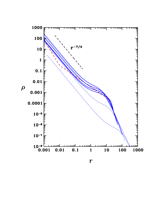
Figure 8: Black hole influence on SIDM halo evolution: snapshots of the density profile at selected times. The lower dashed red line shows the density at time $t=0$. Successively higher solid blue curves show the density at $t=18.09,61.45,97.95$ and $294.8$ (gravothermal collapse). Successively lower dotted blue curves show the density at $t=539.5,2.527\times 10^{3}$ and $2.938\times 10^{4}$ (re-expansion). The upper dashed black line shows the slope for the steady-state BW cusp solution. All quantities are in nondimensional units (see Eq. 45).

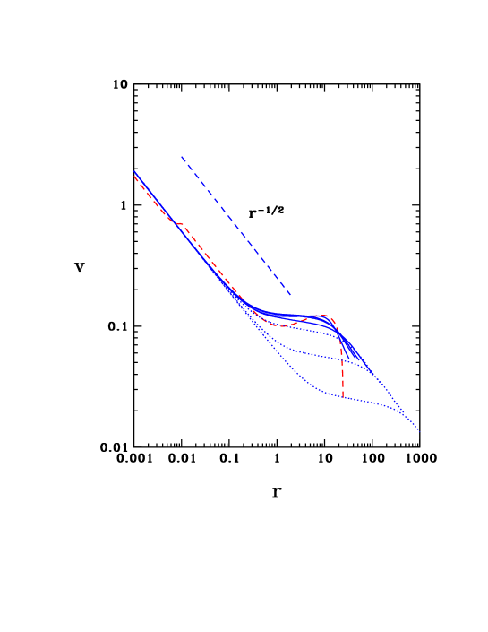
Figure 9: Black hole influence on SIDM halo evolution: snapshots of the velocity dispersion profile at the same selected times depicted in Fig. 8. The straight dashed black curve shows the slope for the steady-state BW cusp solution. All quantities are in nondimensional units.

We use 281 logarithmically spaced grid points spanning seven decades in M to solve the system of equations. The evolution equation for $s$ was integrated implicitly using Eq. (47). Results are summarized in Figs. 8 and  9.

Fig. 8 shows that early on the initial central spike evolves to a standard weakly-collisional cusp around the black hole. For $a=4$ the cusp exhibits the usual BW profile. This happens early because the relaxation time is shortest in the cusp: $t_{r}(r_{h})/t_{r0}=0.11$, where $t_{r}(r_{h})$ is the initial relaxation time at $r=r_{h}$. Shortly afterwards the cuspy NFW density profile tends to smooth out and develop a flatter core outside the cusp. For the period $0\lesssim t/t_{0}\lesssim 295$ the cluster undergoes gravothermal core collapse. For $t/t_{0}\gtrsim 295$ the density in the black hole cusp generates enough heat to eventually reverse core collapse and drive re-expansion of the halo, as predicted.

The velocity dispersion shown in Fig. 9 quickly relaxes to the anticipated BW solution $v^{2}\approx(4/11)M_{h}/r$ in the BH cusp. The dispersion flattens out outside the black hole cusp as a flatter, nearly isothermal density core grows around the cusp. As the the halo expands the velocity dispersion in the core steadily decreases in magnitude, as required by the virial theorem in an expanding, self-gravitating system, and the black hole cusp region grows in time.

III General Relativistic Treatment

The above applications demonstrate the utility of the hydrodynamic conduction approximation for tracking the secular evolution of weakly-collisional, self-gravitating, $N$-body systems in Newtonian gravitation. This motivates us to develop a similar approach in general relativity for virialized systems with strong gravitational fields and constituents moving at velocities approaching the speed of light. We previously provided such an approach to study the special case of steady-state SIDM cusps around massive black holes in halo centers Shapiro and Paschalidis (2014). Here we develop the formalism to track the time-dependent evolution of more general, weakly-collisional, spherical systems. Our treatment, albeit approximate, is designed to fill a gap, as as we are not aware of any other approach that has been employed to treat relativistic systems in this physical regime.

The starting point of our analysis is the metric of a quasistatic, spherical spacetime, which may be written as

$$ds^{2}=-e^{2\Phi}dt^{2}+e^{2\Lambda}dr^{2}+r^{2}d\Omega^{2},$$ (49)

where $e^{2\Lambda}\equiv 1/(1-2M(r)/r)$ and $M(r)$ is the total mass-energy of the configuration inside radius $r$. The relativistic versions of the Newtonian hydrostatic equilibrium Eqs. (1) and (2) are the TOV equations,

$$\frac{\partial M(r)}{\partial r}=4\pi r^{2}\rho,$$ (50)

$$\frac{\partial P}{\partial r}=-(\rho+P)\frac{M(r)+4\pi r^{3}P}{r(r-2M(r))}$$ (51)

and

$$\frac{\partial\Phi}{\partial r}=\frac{M(r)+4\pi r^{3}P}{r(r-2M(r))},$$ (52)

where $\rho$ is the total mass-energy density. The evolution of the system is again governed by the entropy equation, whereby Eq. (3) now becomes

$$\frac{d\rho}{d\tau}-\frac{\rho+P}{n}\frac{dn}{d\tau}=nT\frac{ds}{d\tau}=-\nabla_{a}q^{a}-a_{a}q^{a}=0,$$ (53)

where $\tau$ is proper time, $n$ is the proper particle number density, $T$ is the kinetic temperature, $a^{a}$ is the particle four-acceleration, and $q^{a}$ is the heat flux four-vector. Here we adopt the classical Eckart formulation of relativistic conduction Eckart (1940) (see also Misner et al. (1973)) which is adequate for illustrative purposes, leaving for future implementation more refined formulations that address the issue of noncausality and other subtleties. We follow our analysis in Ref Shapiro and Paschalidis (2014) and model the particles (stars or SIDM) as a perfect, nearly collisionless, relativistic gas where at each radius all the particles have the same local speed but move isotropically. We may then set at each radius $P\equiv nk_{B}T=\rho v^{2}$, where $k_{B}$ is Boltzmann’s constant and $v$ is the one-dimensional velocity dispersion measured by an observer in a static, orthonormal frame. We also have $\rho=\gamma\rho_{0}$, where $\rho_{0}=mn$ is the rest-mass density, $m$ is the particle mass and $\gamma=1/(1-3v^{2})^{1/2}$. These relations give $k_{B}T=\gamma mv^{2}$. Eq. (53) may then be written as

$$\rho v^{2}\frac{d}{d\tau}\ln\left[\frac{(\gamma^{2}-1)^{3/2}}{\rho_{0}}\right]=-\nabla_{a}q^{a}-a_{a}q^{a}.$$ (54)

For a virialized system in a (quasi-)static, spherical gravitational field the only nonzero component of $q^{a}$ is $q^{r}$, where

$$q_{r}=-\frac{\kappa}{|g_{00}|^{1/2}}\frac{\partial\left(T|g_{00}|^{1/2}\right)}{\partial r},$$ (55)

and where $\kappa$ is the effective thermal conductivity and $g_{00}=-e^{2\Phi}$. We determine $\kappa$ for our weakly-collisional (LMFP) systems by first considering the conductivity of a relativistic, strongly-collisional (SMFP) gas of hard-spheres Cercignani and Kremer (2002):

$$\kappa=\frac{3}{64\pi}\frac{k_{B}}{\sigma_{h}}\frac{(\zeta+5G-G^{2}\zeta)^{2}\zeta^{4}K_{2}(\zeta)^{2}}{(\zeta^{2}+2)K_{2}(2\zeta)+5\zeta K_{3}(2\zeta)}.$$ (56)

In the above equation $\zeta=m/k_{B}T$, $K_{n}$ is a modified Bessel function of the second kind, $G=K_{3}(\zeta)/K_{2}(\zeta)$, and $\sigma_{h}=d^{4}/4$, where $d$ is the sphere diameter. Next we write $\sigma_{h}$ in terms of the mean-free path $\lambda$, for which

$$\lambda=\tau_{c}v_{m}=\frac{1}{4\pi\sigma_{h}n}\left[\frac{\gamma^{2}}{1+\gamma^{2}}\right]^{1/2},$$ (57)

where $v_{m}=\sqrt{3}v$ is the mean three-dimensional speed and $\tau_{c}$ is the collision time Anderson and Witting (1974). We then substitute $\lambda$ for $\sigma_{h}$ in Eq. (56), using Eq. (57), and, following the prescription in Refs Lynden-Bell and Eggleton (1980) and  Spitzer, Jr. (1987) for modifying the SMFP result to estimate the conductivity in a weakly-interacting (LMFP) gas, we multiply $\lambda$ by $(H/\lambda)(H/v_{m}t_{r})$.

In nonrelativistic (NR) regions where $\zeta\gg 1$, $\gamma\approx 1$ and $\rho\approx\rho_{0}$, this prescription yields

$$\kappa\approx\frac{75}{64}(2\pi)^{1/2}\rho_{0}v\lambda\frac{k_{B}}{m}\rightarrow\frac{75}{64}\left(\frac{2\pi}{3}\right)^{1/2}\rho_{0}\frac{H^{2}}{t_{r}}\frac{k_{B}}{m}\ \ \ \ ({\rm NR})$$ (58)

which, together with Eq. (55) and the Newtonian relations $q_{r}\approx L/4\pi r^{2}$ and $g_{00}\approx-1$ leads to Eq. (8) for the hard-sphere value of $b=(25/64)\sqrt{2\pi/3}=0.565$ quoted previously. The appropriate value of $t_{r}$ is given by Eq. (13) for stars and by Eq. (42) for SIDM particles. We again note that Ref Spitzer, Jr. (1987) adopts $b=0.45$ as a better fit to more detailed models of Newtonian, isotropic star cluster evolution. We also note that we should set $\eta=\sqrt{6}=2.44$ in Eq. (42) for SIDM particles moving isotropically at a locally constant speed $v_{m}$. The value of the scale height $H$ to assign already has been discussed in Section II, below Eq. (8)

In extreme relativistic (ER) regions where $\zeta\ll 1$, $v_{m}\rightarrow 1$ and $\gamma\gg 1$ we have

$$\kappa\approx 2\lambda\rho_{0}\frac{k_{B}}{m}\rightarrow 2\rho_{0}\frac{H^{2}}{t_{r}}\frac{k_{B}}{m}\ \ \ \ ({\rm ER})$$ (59)

Here $t_{r}$ for a relativistic SIDM gas may be approximated by the collision time $\tau_{c}$:

$$t_{r}\approx\frac{1}{\sigma\rho_{0}v}\left[\frac{\gamma^{2}}{1+\gamma^{2}}\right]^{1/2}\rightarrow\frac{1}{\sigma\rho_{0}}\ \ \ \ ({\rm ER\ SIDM}),$$ (60)

where $\sigma$ (cross section per unit mass) was defined in Eq. (42). The relaxation time for repeated, small-angle scattering for stars in a relativistic cluster is calculated in Appendix A, and is given by

$$t_{r} \approx \frac{3^{3/2}v^{3}}{8\pi m\rho_{0}\ln{(0.4N)}}\left(\frac{\gamma^{2}}{1+6\gamma^{2}v^{2}}\right)^{2},$$ (61)

$$\rightarrow \frac{1}{32\pi m\rho_{0}\ln(0.4N)}\ \ \ \ ({\rm ER\ stars}),$$ (62)

where $v\rightarrow 1/\sqrt{3}$ in the ER limit.

We note that the conductivity described above only takes into account thermal transport generated by elastic collisions between particles. However, there are other, dissipative processes that may contribute to the flux of kinetic energy. In dense clusters of compact stars, for example, these processes include gravitational radiation, specifically gravitational bremsstrahlung, leading to the dissipative formation of binaries and their subsequent merger Zel’dovich and Podurets (1966); Quinlan and Shapiro (1987, 1989). Also important in dense stellar systems are stellar collisions and mergers, as well as binary heating (see  Spitzer, Jr. (1987); Quinlan and Shapiro (1990); Heggie and Aarseth (1992) and references therein). In SIDM halos, there also may be particle annihilation. These dissipative processes can be especially important when the particle velocities become relativistic, although when the cores of virialized, large N-body systems secularly evolve to a sufficiently high central redshift ($\gtrsim 0.5$) they typically become unstable to dynamical collapse, as suggested by Zel’dovich & Podurets Zel’dovich and Podurets (1966) and demonstrated by Shapiro & Teukolsky Shapiro and Teukolsky (1985a, b, 1986, 1992)(but see  Rasio et al. (1989) for a counterexample). In any case it is possible to incorporate such effects by, e.g., adding appropriate heating and cooling terms on the right-hand side of Eq. (53), but such an extension we shall omit in this preliminary analysis.

Evaluating Eq. (54) using $a_{r}=\nabla_{r}\ln|g_{00}|^{1/2}=\partial_{r}\Phi$, Eqs. (49) and (55) yield

$$\rho v^{2}\frac{d}{d\tau}\ln\left[\frac{(\gamma^{2}-1)^{3/2}}{\rho_{0}}\right] = \frac{1}{e^{\Phi+\Lambda}r^{2}}\partial_{r}\left[\kappa e^{-\Lambda}r^{2}\partial_{r}(Te^{\Phi})\right]$$ (63)

$$+ \frac{\kappa}{e^{\Phi+2\Lambda}}\partial_{r}\left(Te^{\Phi}\right)\partial_{r}\Phi.$$ (64)

In some numerical applications it can prove helpful to employ a Lagrangian variable as the independent coordinate, as we did in our Newtonian treatment. The logical choice is the rest-mass $M_{0}(r)$, where

$$\frac{\partial M_{0}}{\partial r}=4\pi r^{2}\rho_{0}e^{\Lambda}.$$ (65)

The resulting set of equations then becomes

$$\frac{\partial M}{\partial M_{0}}=\gamma(1-2M/r)^{1/2},$$ (66)

$$\frac{\partial r}{\partial M_{0}}=\frac{\gamma(1-2M/r)^{1/2}}{4\pi r^{2}\rho},$$ (67)

$$\frac{\partial P}{\partial M_{0}}=-(\rho+P)\frac{M+4\pi r^{3}P}{r(r-2M)}\frac{\partial r}{\partial M_{0}},$$ (68)

$$\frac{\partial\Phi}{\partial M_{0}}=\frac{M+4\pi r^{3}P}{r(r-2M)}\frac{\partial r}{\partial M_{0}},$$ (69)

$$\rho v^{2}\frac{\partial}{\partial\tau}\ln\left[\frac{(\gamma^{2}-1)^{3/2}}{\rho_{0}}\right]=\ \ \ \ \ \ \ \ \ \ \ \$$ (70)

$$\frac{1}{e^{\Phi+\Lambda}r^{2}}\partial_{M_{0}}\left[\kappa e^{-\Lambda}r^{2}\partial_{M_{0}}(Te^{\Phi})\frac{\partial M_{0}}{\partial r}\right]\left(\frac{\partial M_{0}}{\partial r}\right)$$ (71)

$$+\frac{\kappa}{e^{\Phi+2\Lambda}}\partial_{M_{0}}\left(Te^{\Phi}\right)\partial_{M_{0}}\Phi\left(\frac{\partial M_{0}}{\partial r}\right)^{2}.$$

The last (evolution) equation reduces to

$$\begin{split}\rho v^{2}\frac{\partial}{\partial t}\ln\left[\frac{(\gamma^{2}-1)^{3/2}}{\rho_{0}}\right]&=\frac{4\pi\rho}{\gamma}~{}\partial_{M_{0}}\left[\frac{\kappa 4\pi\rho r^{4}}{\gamma}\partial_{M_{0}}(Te^{\Phi})\right]\\ &+\frac{\kappa(4\pi\rho r^{2})^{2}}{\gamma^{2}}\partial_{M_{0}}(Te^{\Phi})~{}\partial_{M_{0}}\Phi.\hskip 113.81102pt\end{split}$$ (72)

In obtaining the final form of the evolution equation we used the relation $\partial_{\tau}\approx e^{-\Phi}\partial_{t}$, which holds since the mean fluid velocity is everywhere negligible in a virialized, spherical, quasistatic system. By implementing Eq. (72) the evolution advances on hypersurfaces of constant coordinate time $t$ (proper time at infinity).

There are then seven unknowns – $M,r,P,\Phi,\rho,\rho_{0}$, and $v$ (or $T$) – that are determined as functions of $M_{0}$ by solving the five relations Eqs. (66) -(72) and using the two auxiliary (equation of state) relations for $P$ and $\rho_{0}$. The kinetic heat flux generated by the interactions can be calculated from

$$\frac{L}{4\pi r^{2}}=|q^{a}q_{a}|^{1/2}=|q_{r}|(1-2M/r)^{1/2},$$ (73)

using Eq. (55).

A subset of the relativistic equations was employed in Ref Shapiro and Paschalidis (2014) to solve for the steady-state distribution of matter in the cusp around a massive black hole a the center of a weakly-collisional clusters of particles. Included in this study were star clusters and SIDM halos. There the central mass of the black hole dominated the cusp and the spacetime was static Schwarzschild. Applications involving the full set of equations to study clusters that secularly evolve into the relativistic regime are planned for the future.

*

Appendix A Relaxation Timescale for Relativistic Gravitational Encounters

Here we provide an approximate calculation of the relaxation timescale due to the cumulative effect of multiple, small-angle, gravitational encounters in a cluster of (point) particles moving at relativistic speeds. We begin by treating the scattering of one test star, $m$, taken at rest, by another star $M$ moving at speed V relative the first. Since we are only interested in small-angle deflections, which are caused by distant encounters, we can take the moving star $M$ to follow a straight line trajectory at an impact parameter $b\gg M$ from the test star. We then adopt the impulse approximation to determine the motion imparted to the test star by the gravitational field of the moving star. We take the trajectory of the moving star to be along the $z$-axis, $z=Vt$, and the test star to lie along the $x$-axis at $x=b$. The impulse, imparted to the test star by the distant, weak field of the moving star, results in a velocity $\Delta v^{\perp}_{m}\ll 1$ perpendicular to the trajectory of the moving star along the $-x$ direction. This velocity may calculated from the Newtonian equation of motion acting on the test star:

$$\frac{d^{2}x}{dt^{2}}=-\frac{\partial\Phi_{N}}{\partial x},$$ (74)

where $\Phi_{N}=-h_{00}/2$ is the Newtonian potential arising from the moving star $M$ and $h_{00}$ is the leading order perturbation to the flat spacetime metric, $g_{ab}=\eta_{ab}+h_{ab}$ induced by $M$. Here $\eta_{ab}$ is the Minkowski metric. The perturbation $h_{a^{\prime}b^{\prime}}$ at the test star in a frame in which $M$ at rest is easily obtained from linear general relativity (see Misner et al. (1973), Exercise 18.3),

$$h_{0^{\prime}0^{\prime}} = h_{x^{\prime}x^{\prime}}=h_{y^{\prime}y^{\prime}}=h_{z^{\prime}z^{\prime}}=\frac{2M}{r^{\prime}},$$ (75)

$$h_{a^{\prime}b^{\prime}} = 0,\ \ \ a^{\prime}\neq b^{\prime},$$ (76)

where $r^{\prime}=(b^{2}+V^{2}t^{\prime 2})^{1/2}$. The perturbation $h_{00}$ appearing in Eq. (74) is then obtained from $h_{a^{\prime}b^{\prime}}$ above by performing a Lorentz boost back to the initial rest frame of the test star, using $t^{\prime}=\gamma(t-Vz)=\gamma t$, where $\gamma=1/(1-V^{2})^{1/2}$. This yields

$$\Phi_{N}=-\frac{h_{00}}{2}=-\frac{M}{(b^{2}+\gamma^{2}V^{2}t^{2})^{1/2}}\left(2\gamma^{2}V^{2}+1)\right).$$ (77)

Inserting Eq. (77) into Eq. (74) and integrating $d^{2}x/dt^{2}$ from $t=-\infty$ to $t=+\infty$ gives

$$\Delta v^{\perp}_{m}=\frac{2M}{bV}\frac{(1+2\gamma^{2}V^{2})}{\gamma}.$$ (78)

The momentum imparted to the test star along $-x$ is $P^{\perp}_{m}=\gamma_{m}m\Delta v^{\perp}_{m}\approx m\Delta v^{\perp}_{m}$, so by momentum conservation $M$ acquires a momentum $P^{\perp}_{M}=\gamma M\Delta v^{\perp}_{M}=-P^{\perp}_{m}$ along $+x$. This gives for the velocity imparted to $M$

$$\Delta v^{\perp}_{M}=\frac{2m}{bV}\frac{1+2\gamma^{2}V^{2}}{\gamma^{2}}.$$ (79)

We note that Eq. (79) reduces to the correct Newtonian result for low velocities,

$$\Delta v^{\perp}_{M}\approx\frac{2m}{bV},\ \ \ \ V\ll 1.$$ (80)

For high velocities Eq. (79) gives

$$\Delta v^{\perp}_{M}\approx\frac{4m}{b},\ \ \ \ V\rightarrow 1,$$ (81)

for which the resulting deflection angle is familiar from light bending,

$$\tan\alpha\approx\alpha\approx\frac{\Delta v^{\perp}_{M}}{V}\approx\frac{4m}{b},\ \ \ \ V\rightarrow 1.$$ (82)

Assuming that $M$ receives repeated, randomly-oriented impulses from multiple perturbers in time $\Delta t$, its cumulative, mean-squared perpendicular velocity kick becomes

$$\langle(\Delta v^{\perp}_{M})^{2}\rangle = \sum_{i}(\Delta v^{\perp}_{M})_{i}^{2}$$ (83)

$$\rightarrow \int_{b_{min}}^{b_{max}}\left(\frac{2m}{bV}\frac{1+2\gamma^{2}V^{2}}{\gamma^{2}}\right)^{2}dN_{p}$$ (84)

$$= \frac{8\pi m^{2}n\Delta t}{V}\ln{\left(\frac{b_{max}}{b_{min}}\right)}\left(\frac{1+2\gamma^{2}V^{2}}{\gamma^{2}}\right)^{2},~{}$$ (85)

where $dN_{p}=n(V\Delta t)(2\pi bdb)$ is the number of perturbers and $n$ is their number density. Here $b_{max}$ is the characteristic scale of the system, while $b_{min}$ is the impact parameter corresponding to large-angle ($\pi/2$) scattering. The relaxation time $t_{r}$ can then be defined as the time $\Delta t$ required for the cumulative perpendicular velocity kick to equal the initial velocity, $\langle(\Delta v^{\perp}_{M})^{2}\rangle=V^{2}$, which gives

$$t_{r}\approx\frac{V^{3}}{8\pi m\rho_{0}\ln{\left(\frac{b_{max}}{b_{min}}\right)}}\left(\frac{\gamma^{2}}{1+2\gamma^{2}V^{2}}\right)^{2}.$$ (86)

For most applications it is reasonable to approximate the logarithmic factor as in Ref Spitzer, Jr. (1987) for Newtonian clusters: $\ln(b_{max}/b_{min})\sim\ln(0.4N)$, where N is the total number of stars. Even for relativistic systems, we expect that $b_{min}\sim m$ and, by the virial theorem, $(Nm)/b_{max}\sim V^{2}\sim 1$, for which $b_{max}/b_{min}\sim N\gg 1$. Setting $V^{2}=v_{m}^{2}=3v^{2}$ gives

$$t_{r}\approx\frac{3^{3/2}v^{3}}{8\pi m\rho_{0}\ln{(0.4N)}}\left(\frac{\gamma^{2}}{1+6\gamma^{2}v^{2}}\right)^{2}.$$ (87)

We observe that in the nonrelativistic limit Eq. (87) gives a relaxation time within a factor of two of the value quoted in Eqs. (13) and Ref Spitzer, Jr. (1987). In the highly relativistic limit Eq. (87) gives a time that scales similarly with $v$ and $\rho_{0}$ and is just a numerical factor (36) times smaller than the nonrelativistic value.

References

- Lynden-Bell and Eggleton (1980) D. Lynden-Bell and P. P. Eggleton, Mon. Not. R. Astro. Soc. 191, 483 (1980).
- Spitzer, Jr. (1987) L. Spitzer, Jr., Dynamical Evolution of Globular Clusters (Princeton, NJ, Princeton University Press, 1987).
- Bettwieser and Sugimoto (1984) E. Bettwieser and D. Sugimoto, Mon. Not. R. Astro. Soc. 208, 493 (1984).
- Bettwieser and Inagaki (1985) E. Bettwieser and S. Inagaki, Mon. Not. R. Astro. Soc. 213, 473 (1985).
- Goodman (1987) J. Goodman, Astrophys. J. 313, 576 (1987).
- Heggie and Ramamani (1989) D. C. Heggie and N. Ramamani, Mon. Not. R. Astro. Soc. 237, 757 (1989).
- Balberg et al. (2002) S. Balberg, S. L. Shapiro, and S. Inagaki, Astrophys. J. 568, 475 (2002).
- Shapiro and Paschalidis (2014) S. L. Shapiro and V. Paschalidis, Phys. Rev. D 89, 023506 (2014).
- Ahn and Shapiro (2005) K. Ahn and P. R. Shapiro, Mon. Not. R. Astro. Soc. 363, 1092 (2005).
- Lightman and Shapiro (1978) A. P. Lightman and S. L. Shapiro, Reviews of Modern Physics 50, 437 (1978).
- Shapiro (1985) S. L. Shapiro, in Dynamics of Star Clusters, IAU Symposium, Vol. 113, edited by J. Goodman and P. Hut (1985) pp. 373–412.
- Elson et al. (1987) R. Elson, P. Hut, and S. Inagaki, Ann. Rev. Astron. Astrophys. 25, 565 (1987).
- Binney and Tremaine (1987) J. Binney and S. Tremaine, Galactic Dynamics (Princeton, NJ, Princeton University Press, 1987).
- Vasiliev (2015) E. Vasiliev, Mon. Not. R. Astro. Soc. 446, 3150 (2015).
- Zel’dovich and Podurets (1966) Y. B. Zel’dovich and M. A. Podurets, Soviet Astr. 9, 742 (1966).
- Shapiro and Teukolsky (1985a) S. L. Shapiro and S. A. Teukolsky, Astrophys. J. 298, 34 (1985a).
- Shapiro and Teukolsky (1985b) S. L. Shapiro and S. A. Teukolsky, Astrophys. J. 298, 58 (1985b).
- Shapiro and Teukolsky (1986) S. L. Shapiro and S. A. Teukolsky, Astrophys. J. 307, 575 (1986).
- Shapiro and Teukolsky (1992) S. L. Shapiro and S. A. Teukolsky, Royal Society of London Philosophical Transactions Series A 340, 365 (1992).
- Rees (1984) M. J. Rees, Ann. Rev. Astron. Astrophys. 22, 471 (1984).
- Shapiro and Teukolsky (1985c) S. L. Shapiro and S. A. Teukolsky, Astrophys. J. Lett. 292, L41 (1985c).
- Quinlan and Shapiro (1987) G. D. Quinlan and S. L. Shapiro, Astrophys. J. 321, 199 (1987).
- Quinlan and Shapiro (1989) G. D. Quinlan and S. L. Shapiro, Astrophys. J. 343, 725 (1989).
- Balberg and Shapiro (2002) S. Balberg and S. L. Shapiro, Phys. Rev. Lett. 88, 101301 (2002).
- Hailey et al. (2018) C. J. Hailey, K. Mori, F. E. Bauer, M. E. Berkowitz, J. Hong, and B. J. Hord, Nature (London) 556, 70 (2018).
- Morris (1993) M. Morris, Astrophys. J. 408, 496 (1993).
- Miralda-Escudé and Gould (2000) J. Miralda-Escudé and A. Gould, Astrophys. J. 545, 847 (2000).
- Freitag et al. (2006) M. Freitag, P. Amaro-Seoane, and V. Kalogera, Astrophys. J. 649, 91 (2006).
- Generozov et al. (2018) A. Generozov, N. C. Stone, B. D. Metzger, and J. P. Ostriker, (2018), arXiv:1804.01543 .
- Elbert et al. (2018) O. D. Elbert, J. S. Bullock, and M. Kaplinghat, Mon. Not. R. Astro. Soc. 473, 1186 (2018).
- Antonini and Rasio (2016) F. Antonini and F. A. Rasio, Astrophys. J. 831, 187 (2016).
- Abbott et al. (2016) B. P. Abbott et al., Phys. Rev. Lett. 116, 061102 (2016).
- Abbott et al. (2017) B. P. Abbott et al., Astrophys. J. Lett. 851, L35 (2017).
- Bahcall and Wolf (1976) J. N. Bahcall and R. A. Wolf, Astrophys. J. 209, 214 (1976).
- Shapiro (1977) S. L. Shapiro, Astrophys. J. 217, 281 (1977).
- Marchant and Shapiro (1980) A. B. Marchant and S. L. Shapiro, Astrophys. J. 239, 685 (1980).
- Duncan and Shapiro (1982) M. J. Duncan and S. L. Shapiro, Astrophys. J. 253, 921 (1982).
- Vasiliev (2017) E. Vasiliev, Astrophys. J. 848, 10 (2017).
- Navarro et al. (1997) J. F. Navarro, C. S. Frenk, and S. D. M. White, Astrophys. J. 490, 493 (1997).
- Clayton (1968) D. D. Clayton, Principles of Stellar Evolution and Nucleosynthesis (New York: McGraw-Hill, 1968).
- Shapiro and Teukolsky (1983) S. L. Shapiro and S. A. Teukolsky, Black Holes, White Dwarfs, and Neutron Stars: The Physics of Compact Objects (New York, Wiley, 1983).
- Shapiro and Lightman (1976) S. L. Shapiro and A. P. Lightman, Nature (London) 262, 743 (1976).
- Reif (1965) F. Reif, Fundamentals of Statistical and Thermal Physics (New York, McGraw-Hill, 1965).
- Lifshitz and Pitaevskii (1981) E. M. Lifshitz and L. P. Pitaevskii, Physical kinetics (Oxford, Pergamon Press, 1981).
- Gondolo and Silk (1999) P. Gondolo and J. Silk, Phys. Rev. Lett. 83, 1719 (1999).
- Vasiliev (2007) E. Vasiliev, Phys. Rev. D 76, 103532 (2007).
- Shapiro and Shelton (2016) S. L. Shapiro and J. Shelton, Phys. Rev. D 93, 123510 (2016).
- Eckart (1940) C. Eckart, Phys. Rev. 58, 919 (1940).
- Misner et al. (1973) C. W. Misner, K. S. Thorne, and J. A. Wheeler, Gravitation (San Francisco, W.H. Freeman, 1973).
- Cercignani and Kremer (2002) C. Cercignani and G. M. Kremer, The Relativistic Boltzmann Equation: Theory and Applications (Basel: Springer AG, 2002).
- Anderson and Witting (1974) A. L. Anderson and H. R. Witting, Physica 74, 466 (1974).
- Quinlan and Shapiro (1990) G. D. Quinlan and S. L. Shapiro, Astrophys. J. 356, 483 (1990).
- Heggie and Aarseth (1992) D. C. Heggie and S. J. Aarseth, Mon. Not. R. Astro. Soc. 257, 513 (1992).
- Rasio et al. (1989) F. A. Rasio, S. L. Shapiro, and S. A. Teukolsky, Astrophys. J. Lett. 336, L63 (1989).