Quark propagator with two flavors of ${\cal O}(a)$-improved Wilson fermions

Abstract

We compute the Landau gauge quark propagator from lattice QCD with two flavors of dynamical ${\cal O}(a)$-improved Wilson fermions. The calculation is carried out with lattice spacings ranging from 0.06 fm to 0.08 fm, with quark masses corresponding to pion masses $m_{\pi}\approx 420,290$ and 150 MeV, and for volumes of up to $(4.5\,\mathrm{fm})^{4}$. Our ensembles allow us to evaluate lattice spacing, volume and quark mass effects. We find that the quark wave function which is suppressed in the infrared, is further suppressed as the quark mass is reduced, but the suppression is weakened as the volume is increased. The quark mass function $M(p^{2})$ shows only a weak volume dependence. Hypercubic artefacts beyond $O(a)$ are reduced by applying both cylinder cuts and H4 extrapolations. The H4 extrapolation shifts the quark wave function systematically upwards but does not perform well for the mass function.

I Introduction

The quark propagator is one of the fundamental objects of QCD, and contains information regarding several of the core nonperturbative features of the theory, namely dynamical chiral symmetry breaking and the absence of quarks from the physical spectrum (confinement). Specifically, a non-vanishing mass function even in the limit of vanishing bare quark mass is a direct sign of dynamical chiral symmetry breaking, while the absence of asymptotic quark states can be translated to an absence of real poles in the propagator, or equivalently, the lack of a positive spectral representation (see, e.g., the discussions in Roberts and Williams (1994); Fischer (2006); Cloet and Roberts (2014); Eichmann et al. (2016)).

Lattice calculations provide us with an opportunity to study these essentially nonperturbative aspects of the quark propagator. Furthermore, first-principles lattice calculations may be used to validate the assumptions used in other nonperturbative approaches such as Dyson–Schwinger equations (DSEs) and functional renormalization group (FRG) calculations, like the recent studies in Williams (2015); Williams et al. (2016); Cyrol et al. (2018); Aguilar et al. (2018)).

The quark propagator is a gauge dependent quantity, and hence requires a choice of gauge condition. The most commonly used gauge, both in lattice and DSE or FRG calculations is the Landau gauge, but other gauge conditions, including Coulomb gauge, maximal abelian gauge and general covariant gauges have also been employed.

In the past, after some early studies using Wilson fermions Becirevic et al. (2000a, b); Skullerud and Williams (2001); Skullerud et al. (2001); Boucaud et al. (2003), most studies of the lattice Landau gauge quark propagator have used staggered Bowman et al. (2002); Parappilly et al. (2006); Bowman et al. (2005); Furui and Nakajima (2005) or overlap Bonnet et al. (2002); Zhang et al. (2004, 2005); Kamleh et al. (2005, 2007) fermions. There have also been calculations using chirally improved fermions Schröck (2012), as well as twisted mass Wilson fermions Blossier et al. (2011); Burger et al. (2013). In August and Maas (2013) there is even a lattice study for adjoint fermions but for the gauge group SU(2).

Although calculations with the same quark content, but different fermion discretizations, should agree in the continuum limit, at finite lattice spacing the lattice artifacts may differ widely, and a comparison between different actions remains an important tool on the way to a controlled continuum extrapolation. In this paper, we present a calculation of the quark propagator using gauge configurations with $N_{f}=2$ flavors of ${\cal O}(a)$-improved Wilson fermion for nearly physical quark masses. In our calculation the quark propagator is also ${\cal O}(a)$-improved. Preliminary results were reported in Oliveira et al. (2016).

The paper is organized as follows. In Section II we give the details of our lattice simulations, including the lattice parameters, gauge fixing and extraction of form factors, and outline our tree-level correction procedure. Section III discusses our lattice results. In Section III.2 we discuss in some detail the hypercubic artifacts beyond tree level, and how they may be brought under control. We end with a brief summary in Section IV.

II Simulation details

II.1 Gauge ensembles

For the computation of the quark propagator we take a subset of the gauge ensembles generated by the Regensburg QCD (RQCD) collaboration (see, e.g., Bali et al. (2013, 2014, 2015)) using $N_{f}=2$ nonperturbatively improved Sheikholeslami–Wohlert (clover) fermions Sheikholeslami and Wohlert (1985) and the Wilson action for the gauge sector. In the present work we use three values for the gauge coupling, corresponding to lattice spacings of $a\approx 0.081\,\text{fm}$, $a\approx 0.071\,\text{fm}$ and $a\approx 0.060\,\text{fm}$, and quark masses corresponding to pion masses of $m_{\pi}\approx 420\,\text{MeV}$, $m_{\pi}\approx 290\,\text{MeV}$, and $m_{\pi}\approx 150\,\text{MeV}$, which is almost at the physical point Bali et al. (2013, 2015). Most of the calculations have been carried out on a lattice volume of $32^{3}\times 64$, but the near-physical quark mass ensemble was generated on a larger $64^{4}$ lattice, corresponding to a physical volume of $(4.5\,\textrm{fm})^{4}$. We have also used a $64^{4}$ lattice to check finite volume effects for one of the other parameter choices ($m_{\pi}\approx 290$ MeV). The parameters used are listed in Table 1.

no.	$\beta$	$\kappa$	$V$	$a$ [fm]	$(m_{\pi},m)$ [MeV]	$N_{\text{cfg}}$
I	5.20	0.13596	$32^{3}\!\times\!64$	0.081	$(280,~{}6.2)$	900
II	5.29	0.13620	$32^{3}\!\times\!64$	0.071	$(422,17.0)$	900
III	5.29	0.13632	$32^{3}\!\times\!64$	0.071	$(295,~{}8.0)$	908
IV	5.29	0.13632	$64^{3}\!\times\!64$	0.071	$(290,~{}8.0)$	750
V	5.29	0.13640	$64^{3}\!\times\!64$	0.071	$(150,~{}2.1)$	400
VI	5.40	0.13647	$32^{3}\!\times\!64$	0.060	$(426,18.4)$	900

Table 1: Lattice parameters used in this study. The lattice spacings $a$ and pion masses $m_{\pi}$ are taken from Bali et al. (2014), while $am=1/(2\kappa)-1/(2\kappa_{c})$ is the subtracted bare quark mass obtained using the critical hopping parameters $\kappa_{c}$ from Bali et al. (2014).

For the gauge fixing we used an over-relaxation algorithm which iteratively maximizes the Landau-gauge functional

$$F_{U}[g]=\frac{1}{4V}\sum_{x\mu}\mathfrak{Re}\operatorname{Tr}U^{g}_{x\mu}$$ (1)

with $U^{g}_{x\mu}=g_{x}U_{x\mu}g^{\dagger}_{x+\hat{\mu}}$ and $g_{x}\in SU(3)$. As stopping criterion we used

$$\max_{x}\;\mathfrak{Re}\operatorname{Tr}\left[(\nabla_{\mu}A_{x\mu})(\nabla_{\mu}A_{x\mu})^{\dagger}\right]<10^{-9}$$ (2)

where $A_{x\mu}\equiv\frac{1}{2iag_{0}}(U^{g}_{x\mu}-U_{x\mu}^{g\dagger})|_{\mathrm{traceless}}$ and $\nabla_{\mu}A_{x\mu}\equiv\sum_{\mu}(A_{x\mu}-A_{x-\hat{\mu},\mu})$, as usual. This stopping criterion corresponds to demanding an average value over the lattice of $\mathfrak{Re}\operatorname{Tr}\left[(\nabla_{\mu}A_{x\mu})(\nabla_{\mu}A_{x\mu})^{\dagger}\right]\lesssim 10^{-12}$. In this study, we do not attempt to investigate the influence of Gribov copies on the quark propagator.

II.2 $\boldsymbol{O(a)}$-improved Wilson quark propagator

For the Wilson-clover action, the ${\cal O}(a)$-improved quark propagator is given by Sheikholeslami and Wohlert (1985); Heatlie et al. (1991); Skullerud and Williams (2001); Skullerud et al. (2001)

$$S_{\mathrm{rot}}(x,y)=(1+2b_{q}am)\left\langle L(x)M^{-1}_{SW}(x,y)R(y)\right\rangle_{U}\;,$$ (3)

where $M^{-1}_{SW}$ is the inverse Wilson clover-fermion matrix which is rotated from left and right by

$$L(x) \equiv\left[1-c_{q}a\overrightarrow{\not{D}}(x)\right]\;,$$ (5a)

$$R(y) \equiv\left[1+c_{q}a\overleftarrow{\not{D}}(y)\right]\,.$$ (5b)

The improvement coefficients $b_{q}$ and $c_{q}$ should be nonperturbatively determined to remove the ${\cal O}(a)$ errors in the quark propagator completely. We expect however that the deviations from tree level are small and therefore fix them at their tree-level (tl) values, i.e., $b_{q}=c_{q}=1/4$ Heatlie et al. (1991). On the lattice, the bare quark mass is

$$am=\frac{1}{2}\left(\frac{1}{\kappa}-\frac{1}{\kappa_{c}(\beta)}\right)\quad\xrightarrow{\beta\to\infty}\;\frac{1}{2\kappa}-4\equiv am_{0}\,,$$ (6)

where $\kappa_{c}(\beta)$ is the critical hopping parameter. This tl-rotated quark propagator is the one used throughout in this paper. For its computation we use correspondingly rotated point sources at four different source locations (except for the $64^{4}$ lattices, where only two sources were used) and average the data from the different sources.

Note that in Skullerud and Williams (2001); Skullerud et al. (2001), a different improved propagator was also analyzed, but as it was found that this propagator has more severe lattice artifacts beyond ${\cal O}(a)$, we will not consider it here.

II.3 Lattice tree-level corrections

In the continuum, the renormalized Euclidean-space vacuum quark propagator can be written as $S^{ab}(p,\mu)=\delta^{ab}S(p,\mu)$ with

$$S(p,\mu)=\frac{1}{i\not{p}A(p^{2},\mu)+B(p^{2},\mu)}\equiv\frac{Z(p^{2},\mu)}{i\not{p}+M(p^{2})}\,,$$ (7)

where $\mu$ is the renormalization scale. The propagator is completely determined by the two form factors $A(p^{2},\mu)$ and $B(p^{2},\mu)$ or alternatively $Z(p^{2},\mu)$ and $M(p^{2})$, the quark wave and mass function, respectively. Due to multiplicative renormalizability $M$ is renormalization-group invariant (see, e.g., Skullerud and Williams (2001); Pennington (2005)) and in momentum subtraction (MOM) schemes is set equal to the running quark mass $M(\mu^{2})=m_{R}(\mu)$ at some ultraviolet renormalization scale, while $Z(\mu^{2},\mu)=1$.

On a finite lattice with periodic boundary conditions in space and antiperiodic boundary conditions in time for the fermions, the available momenta are discrete and given by

$$p_{i} =\frac{2\pi}{N_{i}a}\left(n_{i}-\frac{N_{i}}{2}\right)\;; n_{i}= 1,2,\cdots,N_{i}\,,$$ (8a)

$$p_{t} =\frac{2\pi}{N_{t}a}\left(n_{t}-\frac{1}{2}-\frac{N_{t}}{2}\right)\;; ,n_{t}= 1,2,\cdots,N_{t}\,,$$ (8b)

where $N_{i}$, $N_{t}$ are the number of lattice points in the spatial and temporal directions, respectively. The lattice quark propagator can still be parametrized by two form factors, for instance $A_{L}(p,a)$ and $B_{L}(p,a)$ which in the asymptotic limit and after renormalization reduce to the corresponding continuum functions, i.e.,

$$A(p^{2},\mu) =\lim_{a\to 0}Z_{2}(\mu,a)A_{L}(p,a)\,,$$ (9a)

$$B(p^{2},\mu) =\lim_{a\to 0}Z_{2}(\mu,a)B_{L}(p,a)\,,$$ (9b)

with the quark wave renormalization constant $Z_{2}(\mu,a)$. Note that for any finite lattice spacing, $A_{L}(p,a)$ and $B_{L}(p,a)$ are not functions of $p^{2}$ alone, but also depend on all the other invariants of the (hypercubic) $H(4)$ symmetry group. We therefore keep $p$ instead of $p^{2}$ in the argument of the lattice form factors. For larger $p$, especially if $ap$ is large, the lattice data will expose a different momentum dependence, aka. “fish-bone structure” which survives the renormalization. Only in the asymptotic limit, where the lattice spacing is sufficiently small such that the lattice structure is irrelevant, do these deviations disappear for any fixed value of the momentum $p$. Improved lattice operators and actions help to improve the convergence towards the continuum.

For commonly used values of $\beta$ these deviations due to the lattice spacing are large when using an unimproved (clover-) Wilson fermion propagator. We therefore use the ${\cal O}(a)$-improved (tl-rotated) lattice Wilson fermion propagator given in Eq. (3), which at tree level reads Skullerud and Williams (2001)

$$S^{(0)}_{\mathrm{rot}}(p,a,m) =\frac{Z_{\mathrm{rot}}^{(0)}(p,a,m)}{i\not{\bar{p}}+M_{\mathrm{rot}}^{(0)}(p,a,m)}\,,$$ (10a)

with

$$Z_{\mathrm{rot}}^{(0)}(p,a,m) =\left(1+\frac{am}{2}\right)\frac{\bar{p}^{2}I_{A}^{2}+I_{B}^{2}}{I_{A}D_{W}}\,,$$ (10b)

$$M_{\mathrm{rot}}^{(0)}(p,a,m) =\frac{I_{B}}{I_{A}}$$ (10c)

and

$$D_{W} \equiv\bar{p}^{2}+[m+M_{W}]^{2}\,,$$ (11a)

$$I_{A} \equiv 1+\frac{am}{2}+\frac{3a^{2}\bar{p}^{2}}{16}+\frac{a^{4}\left(\hat{p}^{2}-\bar{p}^{2}\right)}{4}\,,$$ (11b)

$$I_{B} \equiv m\left(1-\frac{a^{2}\bar{p}^{2}}{16}\right)-\frac{a^{3}}{32}\bar{p}^{2}\hat{p}^{2}+\frac{a^{3}\left(\hat{p}^{2}-\bar{p}^{2}\right)}{2}\,.$$ (11c)

The Wilson mass term $M_{W}=a\hat{p}^{2}/2$ and the lattice momentum functions are

$$\bar{p}_{\mu} \equiv\frac{1}{a}\sin(ap_{\mu})\,,$$ (12)

$$\hat{p}_{\mu} \equiv\frac{2}{a}\sin(ap_{\mu}/2)\,.$$ (13)

Knowledge of the lattice tree-level propagator is of great advantage when one extracts the nonperturbative quark form factors from the lattice data. With appropriate projections one obtains form factors which are exact at tree level. We will see this reduces a large fraction of the lattice artifacts mentioned above.

Following this, we define the (renormalized) nonperturbative quark wave and mass functions as

$$Z(p,\mu,m) =Z_{2}^{-1}(\mu,a)\cdot Z_{L}(p,a,m)$$ (14)

$$Z_{L}(p,a,m) =Z_{\mathrm{rot}}(p,a,m)/Z_{\mathrm{rot}}^{(0)}(p,a,m)$$ (15)

and

$$M_{L}(p,a,m) =\Big{(}M_{\mathrm{rot}}(p)-M_{\mathrm{rot}}^{(-)}(p)\Big{)}\,/\,Z^{\scriptscriptstyle(+)}_{m}(p)$$ (16)

where $M_{\mathrm{rot}}^{(0)}$ has been split into strictly positive and negative terms Skullerud et al. (2001):

$$M^{(0)}_{\mathrm{rot}}(p)\equiv m\underbrace{Z^{(+)}_{m}(p)}_{\geq 1}+\underbrace{M_{\mathrm{rot}}^{(-)}(p)}_{\leq 0}\,.$$ (17)

$Z_{L}$ and $M_{L}$ have the correct form at tree level if $Z_{\mathrm{rot}}=1/A_{\mathrm{rot}}$ and $M_{\mathrm{rot}}=B_{\mathrm{rot}}/A_{\mathrm{rot}}$ are obtained from the usual traces of the lattice data for $S_{\mathrm{rot}}$ [Eq. (3)]:

$$A_{\mathrm{rot}}(p,a,m) =\frac{1}{12\bar{p}^{2}}\operatorname{Tr}\left[\not{\bar{p}}~{}S^{-1}_{\mathrm{rot}}(p,a,m)\right]\;,$$ (18a)

$$B_{\mathrm{rot}}(p,a,m) =\frac{1}{12}\operatorname{Tr}\left[S^{-1}_{\mathrm{rot}}(p,a,m)\right]\,.$$ (18b)

with $\bar{p}$ defined in Eq. (12). In the continuum, the mass function is renormalization-group invariant. Hence $M(p^{2},m)=\lim_{a\to 0}M_{L}(p,a,m)$. We find only a very weak dependence on the lattice spacing in our data, and hence conclude that for our lattice spacings we are close to the limit. To simplify notation, we therefore drop the subscript $L$, when showing lattice data for the mass function.

Here a note on our lattice tree-level corrections of the mass function is in order: Naively one would correct it by subtracting the $p$-dependent part of the lattice tree-level expression, i.e.,

$$M_{\mathrm{sub}}(p)=M_{\mathrm{rot}}(p)-M_{\mathrm{rot}}^{(0)}(p,m)+m\,,$$ (19)

analogously as one would subtract $M_{W}$ in case of the unimproved Wilson quark propagator. Alternatively, one could apply a multiplicative correction, i.e., define the nonperturbative mass function as

$$M_{\mathrm{mul}}(p)=M_{\mathrm{rot}}(p)/Z^{(0)}_{m}(p)$$ (20)

with $M_{\mathrm{rot}}^{(0)}(p)\equiv m\cdot Z^{(0)}_{m}(p)$. However, this approach suffers from cancellation effects when either $M_{\mathrm{rot}}$ or $M_{\mathrm{rot}}^{(0)}$ take values around zero (cf. Fig. 2). It was found in Skullerud et al. (2001) that the “hybrid” tree-level correction in Eqs. (16) and (17) combines the advantages of the additive and multiplicative correction. Hence we use it for the results for $M$ shown below. A comparison with $M_{\mathrm{mul}}(p)$ is shown in the appendix.

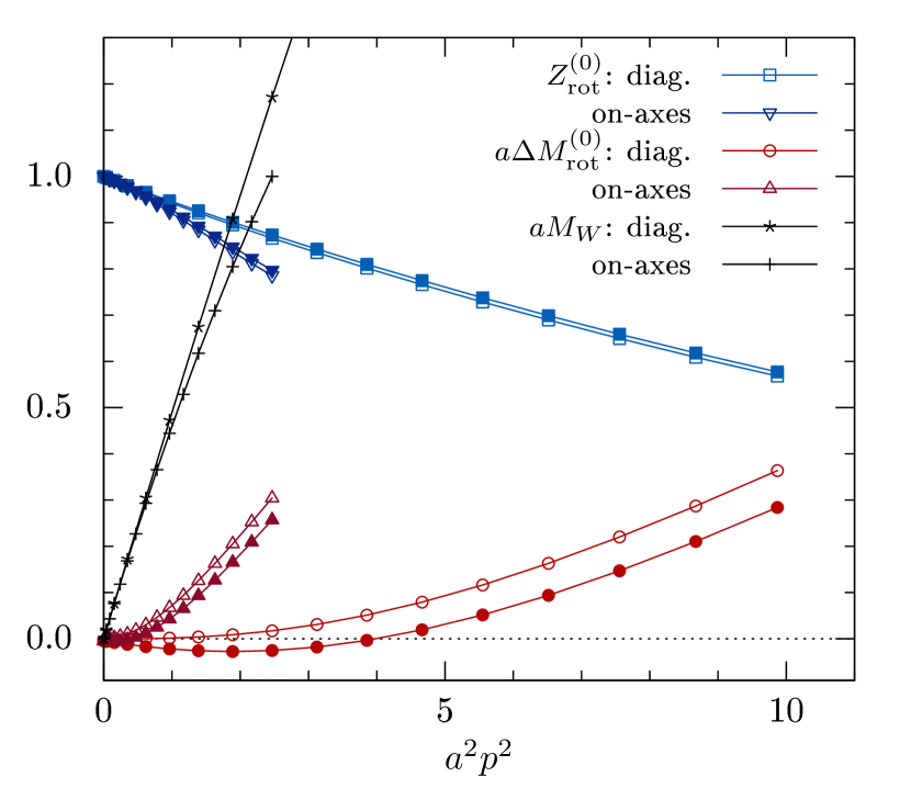
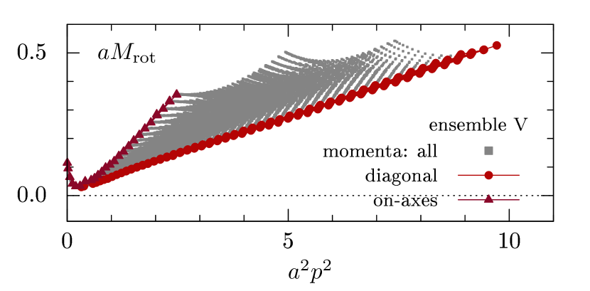
Figure 1: $Z_{\mathrm{rot}}^{(0)}(p)$, $aM_{W}(p)$ and $a\Delta M_{\mathrm{rot}}^{(0)}(p)\equiv aM_{\mathrm{rot}}^{(0)}(p)-am$ versus $a^{2}p^{2}$ for diagonal and on-axes momenta $ap$. Open symbols are for $am=0$, full symbols for $am=0.1$.

Figure 2: Bare uncorrected lattice data for $aM_{\mathrm{rot}}(p)$ versus $a^{2}p^{2}$ for ensemble V (see Table 1). Circles are for (near) diagonal momenta and triangles for (near) on-axis momenta.

For illustrative purposes, we show in Fig. 2 the momentum dependence of $Z_{\mathrm{rot}}^{(0)}$, $a\Delta M_{\mathrm{rot}}^{(0)}\equiv aM_{\mathrm{rot}}^{(0)}-am$ and the Wilson mass term $aM_{W}$, both for diagonal and on-axes momenta $ap$. Filled symbols are for $am=0.1$, open symbols for $am=0$. We see that $a\Delta M_{\mathrm{rot}}^{(0)}$ changes sign depending on $ap$ and $am$, while $Z_{\mathrm{rot}}$ is almost unaffected by the quark mass. Also note that the ${\cal O}(a)$ improvement is already evident at tree-level: $a\Delta M^{(0)}_{\mathrm{rot}}$ increases much less with $ap$ than $aM_{W}$ which dominates the lattice artifacts of the unimproved Wilson (clover-) fermion propagator. On-axes momenta cause larger effects, than momenta along diagonal lattice directions, for which $aM_{\mathrm{rot}}^{(0)}\simeq am$ even up to $ap<2$. Changing the quark mass changes $a\Delta M_{\mathrm{rot}}^{(0)}$ much less than the momentum orientation. Note that for our $\beta$ values, $am=0.1$ corresponds to larger quark masses than we use for our study. Our values for $am$ range from $am=0.00075$ (ensemble V) to $am=0.006135$ (ensemble II). The value of $am$ is hence negligible for the tree-level corrections; only the type momentum orientation matters.

In Fig. 2 we show, as an example, bare uncorrected lattice data for $aM_{\mathrm{rot}}$ for our lightest-quark ensemble V (aka. fishbone plot). The points scatter depending on the size and type of momentum; on-axes momenta show the largest and diagonal momenta the smallest discretization effects. Comparing Fig. 2 and 2 we see the dominant part of these effects is already contained in the tree-level propagator. This explains the effectiveness of applying lattice tree-level corrections, though we also see that the linear $a^{2}p^{2}$ dependence sets in at much lower $a^{2}p^{2}$ than it does for the tree-level curves.

II.4 Beyond lattice tree-level corrections

Using the tl-rotated quark propagator and the tree-level correction helps to drastically reduce the discretization effects. The figures below will clearly evidence this. However, the discretization artifacts are not removed completely. To reduce the remaining hypercubic artifacts, we consider two strategies:

1. Data cuts: We have employed the cylinder cut first described in Leinweber et al. (1999) to select momenta close to the diagonal in 4-momentum space, which have the smallest hypercubic artifacts. We have also considered an alternative cut based on the value of $x\equiv p^{[4]}/p^{[2]}$ (see below), selecting only momenta for which $x<x_{\max}$. The results of this cut are similar to those of the cylinder cut, but the cylinder cut gives a more even distribution of points across the entire momentum range and is hence preferred.

2. H4 extrapolation Becirevic et al. (1999); de Soto and Roiesnel (2007): This will be described in more detail in Section III.2 below.

III Results

III.1 Tree-level corrected data

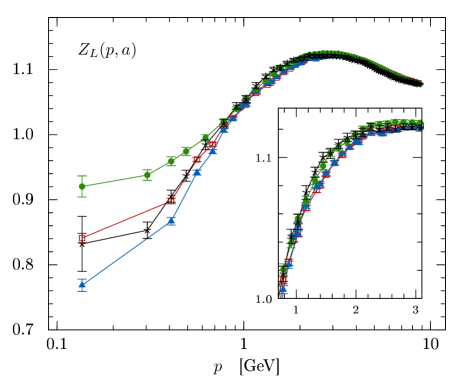
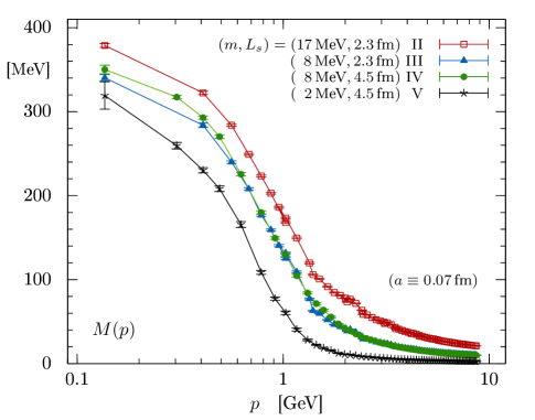
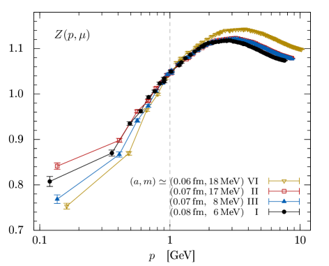
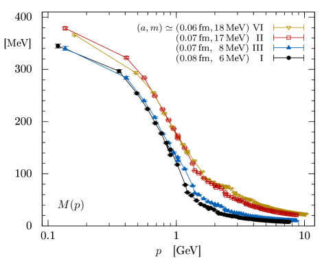
Figure 3: The unrenormalized tree-level corrected wave function $Z_{L}(p,a)$ (left) and the hybrid tree-level corrected mass function $M_{L}(p)$ (right) as a function of $p$. The data are for a fixed lattice spacing ($\beta=5.29$), but different spatial extent $L_{s}$ and quark masses $m$ to demonstrate volume and quark mass effects. The corresponding gauge field ensembles are II, III, IV and V. Momenta are cylinder cut with a radius of 1 lattice momentum unit. The top right legend applies to both plots.

Figure 4: The renormalized tree-level corrected wave function $Z(p,\mu)$ (left) and the hybrid tree-level corrected mass function $M(p)$ (right) as a function of $p$, for our four ensembles on a $32^{3}\times 64$ lattice (I, II, III and VI). They have been renormalized at $\mu=1\,\textrm{GeV}$, relative to the $\beta=5.29$ points ($a=0.07\,\textrm{fm}$). Open symbols refer to data for $m\simeq$ 17–18 MeV; full symbols for $m\simeq$ 6–8 MeV.

We start our discussion of data with the four ensembles at $\beta=5.29$ and focus first on volume and quark mass effects. The tree-level corrected results for $Z(p,a)$ and $M(p)$ are shown in Fig. 4 as a function of $p$. The quark wave function is left unrenormalized ($Z_{2}\equiv 1$), because the data points are for a single $\beta$. As expected, for large momenta the quark mass dependence of $Z$ is negligible; the points for $Z$ almost collapse onto a single curve. For $p<3\,\text{GeV}$, however, deviations grow as $p$ decreases. Between $p=1$ and 2 GeV, both a larger spatial volume and a smaller quark mass value cause points to move up. Interestingly, around $p=1\,\textrm{GeV}$ points for the different sets almost coincide, although no renormalization was applied. For $p<1\,\textrm{GeV}$ deviations grow again towards the infrared, depending on quark mass and volume: at fixed $p$, a larger volume causes $Z$ to move up [compare triangles and circles in Fig. 4 (left)], while a smaller quark mass causes the opposite effect (compare circles to crosses, or squares to triangles). Within our parameter ranges, the quark mass suppression is similar in size to the enhancement with volume.

For the mass function $M(p)$ at $\beta=5.29$ (Fig. 4, right) we see a clear quark mass dependence. Varying $m$ not only changes the offset at large $p$, but also the functional form of $M(p^{2})$. A simple rescaling of $M(p^{2})$ or a subtraction of a finite offset will not collapse the data points onto a single curve. The volume effect for $M(p)$ is small in comparison and actually only resolvable for $p<0.6\,\textrm{GeV}$. A larger volume causes points to move slightly up (compare circles to triangles for $p<0.6\,\textrm{GeV}$).

Next we look at discretization effects for which we compare our $32^{3}\times 64$ data for $\beta=5.20$, 5.29 and 5.40 (ensembles I, II, III and VI). We have to apply a renormalization factor $Z_{2}$, separately for each $\beta$ (see Eq. (14)). For a better comparison with Fig. 4 we again set $Z_{2}\equiv 1$ for $\beta=5.29$ and renormalize the other two sets (I and IV) relative to that. As renormalization point we chose $\mu=1\,\textrm{GeV}$ for which we found the smallest volume and quark mass effects at small $p$. For the same reason we could chose any other point above $3\,\textrm{GeV}$ as well, but for large $p$ we actually expect (and find) discretization effects. Renormalizing there would artificially shift these effects to smaller momenta where they would overlap with volume and quark mass effects. Choosing $\mu=1\,\textrm{GeV}$ is thus optimal for our purposes.

$M$ was not renormalized, because it is renormalization group invariant if lattice discretization effects are removed. We will now analyze these effects.

Our results for $Z(p,\mu)$ and $M(p)$ are shown in Fig. 4 and we clearly see discretization effects for larger $p$. In particular, the non-monotonic behavior of $Z(p,\mu)$, reaching a maximum at $p\sim 3$ GeV and bending down towards larger $p$, is an effect seen in previous studies with Wilson–clover fermions which is absent in studies using other discretizations. By looking at the bare uncorrected data (not shown) we find that the tree-level correction, in combination with the momentum selection (cylinder cut), indeed removes most of the discretization effects. This removal is not complete, as expected, and what remains is seen in Fig. 4. If the removal was complete, the points for $Z$ above 1 GeV would collapse onto a single curve and only at small momentum would deviations due to volume or quark mass effects be seen.

   

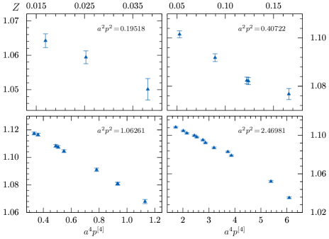
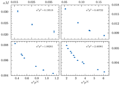
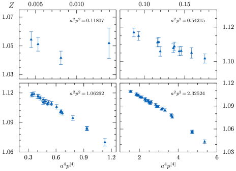
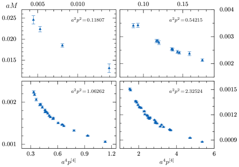
Figure 5: $Z_{L}(p^{2},p^{[4]})$ (left panels) and $aM_{L}(p^{2},p^{[4]})$ (right panels) as a function of $a^{4}p^{[4]}$ at four values of $a^{2}p^{2}$. The top panels show data for $\beta=5.29$, $\kappa=0.13632$ and a $32^{3}\times 64$ lattice, the bottom panels for $\beta=5.29$, $\kappa=0.13640$ and a $64^{4}$ lattice.

Similarly, for $M(p)$ the renormalization group invariance is broken by lattice artifacts. In Fig. 4 (right) we see that the data for $M$ with approximately the same $m$ overlap within errors for $p<1\,\textrm{GeV}$, while for $p>1$ GeV a similar but slightly different $p$-dependence is seen. For the reader’s convenience we have used open and full symbols in Fig. 4 to indicate the respective $m$. Overall, lattice spacing effects for $M$ are smaller than for $Z$.

It is indeed reassuring to see that the bending down of $Z(p,\mu)$ sets in at higher $p$ the finer the lattice (compare the points for ensemble I and VI in Fig. 4). Also, the mass function $M(p)$ falls off for large $p$ such that one can assume that it will approach the perturbative running of the quark mass in the ultraviolet limit if all discretization effects are subtracted. In the infrared momentum limit we see the dynamically generated “constituent” quark mass of about 300–400 MeV, which one would expect. It has been suggested Fischer and Alkofer (2003); Aguilar and Papavassiliou (2011) that $M(p)$ should reach a plateau at small $p$. With our data we can neither confirm nor refute this. We see a slight change of slope at small $p$ for the ensembles III and IV, but data points for much lower $p$ are needed to address this.

III.2 Correction of hypercubic artifacts

Using the tl-rotated quark propagator and the tree-level correction described above, we obtained quark dressing functions for cylinder-cut momenta which show much smaller lattice spacing effects than unimproved and uncorrected data for the clover quark propagator would show. However, the discretization effects are not removed completely. We will now attempt to reduce the remaining hypercubic discretization effects using the (so-called) H4 method Becirevic et al. (1999); de Soto and Roiesnel (2007). Note that our implementation differs slightly from the original proposal.

On the lattice the orthogonal group $O(4)$ of Euclidean space-time is reduced to the hypercubic group $H(4)\subset O(4)$. Consequently, for any lattice spacing, the traces $A_{L}$ and $B_{L}$ [Eq. (18)] are symmetric under $H(4)$ transformations and hence functions of the hypercubic invariants $p^{2}$, $p^{[4]}$, $p^{[6]},p^{[8]},\ldots$ with

$$p^{[2i]}\mathrel{\mathop{:}}=\sum_{\mu}p^{2i}_{\mu}\qquad\forall i=2,3,4,\ldots\;\text{.}$$ (21)

In four dimensions the first four invariants are sufficient. All remaining invariants, and any combination thereof, are functions of those four. In the continuum limit, the renormalized traces $A(\mu^{2},p^{2})$ and $B(\mu^{2},p^{2})$ are functions of $p^{2}$ alone. Therefore, we can assume that to leading order in the lattice spacing $a$ the lattice quark propagator traces $F_{L}=\{A_{L},B_{L}\}$ are of the form de Soto and Roiesnel (2007)

$$F_{L}(a,p)\equiv F_{L}(a^{2},p^{2},p^{[4]},p^{[6]},p^{[8]})~{}\simeq~{}F(a^{2},p^{2})+a^{4}p^{[4]}f_{4}(a^{2},p^{2})+a^{6}p^{[6]}f_{6}(a^{2},p^{2})+a^{8}p^{[8]}f_{8}(a^{2},p^{2})+\ldots\,.$$ (22)

$F(a^{2},p^{2})$ contains all $O(4)$-symmetric terms, i.e., terms which are functions of $a^{2}p^{2}$ and $a^{2}$ only. The “hypercubic” terms describe the leading deviation from $O(4)$ symmetry.

Such an expression (up to the second term) is for example obtained from an $O(a^{2})$ expansion of the 1-loop Wilson quark propagator (see Eq.(4.1) in Constantinou et al. (2009)). There, $F(a^{2},p^{2})$ is the sum of the usual constants, the $\log(a^{2}p^{2})$ term as well as the scaling violations proportional to $a^{2}p^{2}$. The leading hypercubic correction to $A_{L}$ reads $a^{4}p^{[4]}f_{4}(a^{2},p^{2})$ with

$$f^{1l}_{4}(a^{2},p^{2})=\frac{c_{0}(g^{2})+c_{1}(g^{2})\log(a^{2}p^{2})}{a^{2}p^{2}}$$ (23)

where the $c_{i}(g^{2})$’s are functions of the coupling. The log-term in $F(a^{2},p^{2})$ is multiplicatively removed by the respective renormalization constant, while the $a^{2}p^{2}$ and $a^{2}p^{[4]}/p^{2}$ terms vanish in the continuum limit. For any finite $a$ both terms add to the scaling violations, but those due to the hypercubic terms also depend on the momentum direction: they are largest for on-axis momenta and smallest (but non-zero) for cylinder-cut momenta (see again Fig. 2). The H4 method attempts to remove exactly those contributions to the scaling violations.

Our implementation of the H4 method is a modified version of the local H4 method described in de Soto and Roiesnel (2007). There, $f_{4}=c_{0}+c_{1}/p^{2}+c_{2}p^{2}$ and the constants $c_{i}$ are obtained from fits to the data for a range of $p^{2}$. Our fits are performed for individual $p^{2}$, but we allow coefficients to depend on $p^{2}$. That is, we do not fix the form of $f_{4}$ and instead write

$$f_{4}(a^{2},p^{2})=\frac{c(a^{2},p^{2})}{a^{2}p^{2}}\,.$$ (24)

Given that our lattice propagator agrees with the continuum expression to order $\mathcal{O}(a)$, we restrict the expansion to $\mathcal{O}(a^{2})$. We do check, however, whether the fits improve if higher hypercubic terms are included. We will also analyze the functional form of $c(a^{2},p^{2})$.

The H4 method cannot completely remove the lattice artifacts, in particular not the scaling violations in $F(a^{2},p^{2})$. However, our H4 extrapolation is performed on the data after removing the tree-level artifacts as described above. This tree-level correction already drastically reduces the scaling violations in $F(a^{2},p^{2})$ and the hypercubic terms. A subsequent application of the H4 method further reduces the hypercubic part. The bending of the quark dressing at large $a^{2}p^{2}$ should flatten for instance.

For the (tree-level corrected) form factors, $A$ and $B$, and the quark wave function $Z=1/A$, we expect similar hypercubic expansions to hold. If this is the case then the leading hypercubic corrections for the mass function $M=B/A$ should be comparably smaller, in particular if those of $A$ and $B$ are of similar size. We thus expect that higher hypercubic terms dominate the behavior at large $p^{[2i]}$. In the continuum limit $M$ is renormalization-group invariant and so it is also plausible that it may have smaller discretization effects.

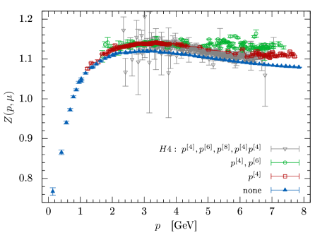
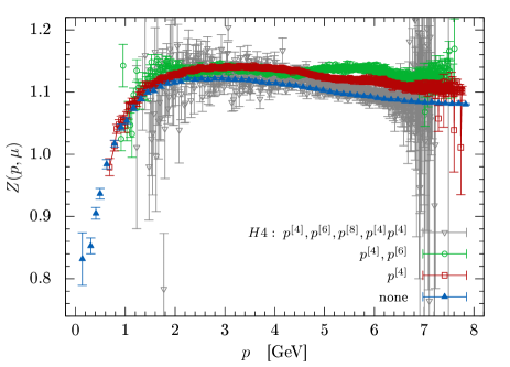
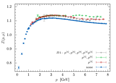
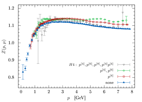
Figure 6: H4-extrapolated quark wave function for $\beta=5.29,\kappa=0.13632,V=32^{3}\times 64$ (left panels) and for $\beta=5.29,\kappa=0.13640,V=64^{4}$ (right panels). The top panels show the raw data before smoothing, while the bottom panels show the results after averaging with a momentum resolution $\epsilon=0.05$ (see text for details). In the legend we list the hypercubic terms included for the fit.

In the next subsection we discuss the results of the H4 method applied to the quark wave function $Z$ and the quark mass function $M$. For the fits we group the lattice data $D_{F}$ for $F=\{Z,M\}$ wrt. the value of $p^{2}$. The number of data points for each $p^{2}_{i}$ varies, hence the statistical error of each fit will vary, too. Our fit parameters are $F(a^{2},p^{2})$ and $c(a^{2},p^{2})$. If higher terms are included in the fit, there is an additional parameter $c_{i}(a^{2},p^{2})$ for each of the terms $p^{[6]}$, $p^{[8]}$ and $p^{[4]}p^{[4]}$. The quality of a fit is monitored by the $\chi^{2}$-function:

$$\chi^{2}(p^{2}_{i})=\\ \sum_{j}\frac{\left[F_{L}(a^{2},p^{2}_{i},p^{[4]}_{j},\ldots)-D_{F}(a^{2},p^{2}_{i},p^{[4]}_{j},\ldots)\right]^{2}}{\sigma^{2}_{F}(p^{2}_{i},p^{[4]}_{j}\ldots)}\,,$$ (25)

where $D_{F}$ denotes the tree-level corrected data for $F=Z$ and $M$, and $F_{L}(a^{2},p^{2}_{i},p^{[4]}_{j},\ldots)$ denotes the H4 expansion in Eq. (22) with $f_{4}(a^{2},p^{2})$ in Eq. (24). The minimization of $\chi^{2}$ is translated into finding the solution of a linear system of equations for $c(a^{2},p^{2})$, which is solved by Gauss-Jordan elimination. Statistical errors are estimated with the bootstrap method with a 67.5% confidence level. The number of bootstrap samples is ten times the number of configurations. Fits with $\chi^{2}/d.o.f.\geqslant 2$ are disregarded.

In the following, for the numerical procedure to measure $Z(p^{2})$ and $M(p^{2})$ we will always assume an exact H4 hypercubic symmetry group, which holds only for $L^{4}$ lattices. The results reported here will also include the asymmetric lattice $32^{3}\times 64$, but given the volume and lattice spacing used in the simulation, we expect the corrections due to the asymmetry to be small — see the analysis and the discussion in Ref. Blossier et al. (2011).

In Fig. 5 we plot the quark wave function and running mass for various $a^{2}p^{2}$ values as a function of $a^{4}p^{[4]}$ for the simulations performed with $\beta=5.29$ on the $32^{4}\times 64$ lattice with $\kappa=0.13632$, corresponding to $m_{\pi}=295$ MeV (upper panels) and on the $64^{4}$ lattice with $\kappa=0.13640$, corresponding to $m_{\pi}=150$ MeV (lower panels). The lattice data show a smooth behavior as a function of $a^{4}p^{[4]}$, with the data for $Z(p^{2})$ suggesting an essentially linear function of $a^{4}p^{[4]}$, while the data for $aM(p^{2})$ show clear deviations from a linear behavior in $a^{4}p^{[4]}$. From the point of view of the H4 method, the observed smooth behavior in the various plots is quite encouraging, suggesting that it is possible to achieve a reliable extrapolation to the O(4) symmetric limit.

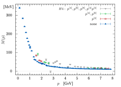
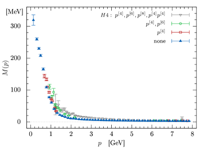
Figure 7: H4-extrapolated running mass function $M(p^{2})$ after binning with a momentum resolution $\epsilon=0.05$ (see text for details), for $\beta=5.29,\kappa=0.13632,V=32^{3}\times 64$ (left) and $\beta=5.29,\kappa=0.13640,V=64^{4}$ (right) As in Fig. 6 we list the hypercubic terms included for the fit.

III.3 Tree-level and H4-corrected data

The top panels of Fig. 6 compare the H4-extrapolated data (open symbols) for the quark wave function with the tree-level corrected data (full triangle) of Fig. 4. We focus again on the ensembles III and V, but the comparison looks similar for the other ensembles. The H4-extrapolated points result from three types of extrapolation: The $p^{[4]}$ points are from extrapolations where the hypercubic corrections are described by $f_{4}(a^{2},p^{2})$ in Eq. (24) alone. Open circles are from extrapolations where a $p^{[6]}$-correction term was included as well. The open triangles are from fits where also terms proportional to $p^{[8]}$ and $p^{[4]}p^{[4]}$ were included. All three extrapolations agree within errors up to $p\simeq 4\,\text{GeV}$ ($pa\simeq 1.5$), but the errors drastically increase when more hypercubic correction terms are included. Note again that points from extrapolations with $\chi^{2}/d.o.f.\geqslant 2$ have been discarded and hence do not appear in Fig. 6.

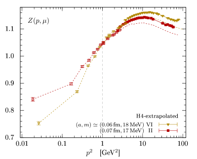
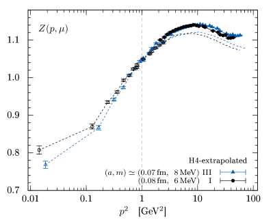
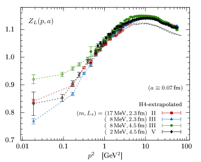
Figure 8: Quark wave function versus $p^{2}$ after tree-level correction (open) and H4 extrapolation (full symbols). Top and middle panel show data for different lattice spacings, $a$, but approximately same quark mass, $m=6\ldots 8\,\text{MeV}$ and $m=17\ldots 18\,\text{MeV}$, respectively. The bottom panel shows data for $a\equiv 0.07\,\text{fm}$ but varying $m$ and volume.

The bottom panels of Fig. 6 show the same comparison as the top but there the points are weighted averages of data from nearby momenta, with weights given by the inverse statistical error. The data binning reduces the statistical fluctuations drastically. We have tried different bin sizes by varying the momentum resolution

$$\epsilon=\frac{|p^{\prime}-p|}{p}$$ (26)

and find that $\epsilon=0.05$ is a reasonable compromise between acceptable uncertainties, a smooth curve and a sufficient number of data points. From the binned data we see that the three types of H4 extrapolations give slightly different results for $p>4\,\text{GeV}$ ($pa>1.5$). We also find that the $p^{[6]}$ term tends to destabilize the fit, yielding an erratic behavior at high momenta. The $64^{4}$ ensemble (V) has smaller statistics as seen in the top panels, but since there is a larger number of $p^{2}$ invariant momentum combinations within each momentum bin, after binning we obtain comparable results.

The H4 extrapolation works well for the quark wave function. For the running quark mass, however, the extrapolations perform much worse — see Fig. 7, where the H4-extrapolated $M(p)$ is shown for the same ensembles as for $Z(p)$ above. In fact, the number of fits with $\chi^{2}/d.o.f.\leq 2$ is significantly smaller for $M(p)$, than it is for $Z(p^{2})$. Only by including all hypercubic terms up to the $p^{[8]}$ and $p^{[4]}p^{[4]}$ terms can reasonable extrapolations be found.

In Fig. 7 we compare the H4-extrapolated with the tree-level corrected data for $M(p^{2})$, again by showing weighted averages of data from nearby momenta ($\epsilon=0.05$). For large $p$, our H4-extrapolation changes the momentum behavior of the tree-level corrected $M(p)$ only slightly, while for smaller $p$ the extrapolated values differ more significantly, in particular between $p=1.3\,\text{GeV}$ and $3\,\text{GeV}$. From the nature of hypercubic artifacts we would expect the opposite trend. Furthermore, the points from the three types of extrapolations do not coincide at small $p$, while they tend to converge onto a single curve with the tree-level corrected (cylinder-cut) data for high $p$. We conclude that our H4-extrapolation fails for $M$ and consider the tree-level corrected data in Fig. 4 and 4 as our final data for $M$.

Our results for $Z$ after tree-level correction and H4 extrapolation ($\epsilon=0.05$) are shown in Fig. 8 (full symbols). If the linear H4 extrapolation in $a^{2}p^{[4]}/p^{2}$ was not successful (i.e. $\chi^{2}/d.o.f.\geq 2$), the tree-level corrected data are shown instead (open symbols). They are the same as in Fig. 4 and 4. To guide the eye and to demonstrate the shift due the H4 extrapolation we have added dashed lines connecting the tree-level corrected points. These points are not shown above $p^{2}\simeq 3\,\text{GeV}^{2}$ in Fig. 8 to improve the visibility of the shift. The points in the two upper panels of Fig. 8 have been renormalized relative to the $a=0.07\,\text{fm}$ data at $\mu=1\,\text{GeV}$. This allows for a better comparison with the bottom panel showing unrenormalized data at fixed lattice spacing ($a=0.07\,\text{fm}$) but different volumes and quark masses.

In Fig. 8 we see that the H4 extrapolation causes an upward shift of all data points above $p^{2}\simeq 2\,\text{GeV}^{2}$. For the heavier quark mass sets (top panel) the H4 extrapolation causes also a slight reduction of the vertical difference for $3\,\text{GeV}^{2}<p^{2}<10\,\text{GeV}^{2}$. For the lighter quark mass this difference is already negligible after tree-level correction. For the single-$a$ data in the bottom panel of Fig. 8 we observe that the points above $p^{2}=1\,\text{GeV}^{2}$ tend to overlap less after H4 extrapolation. This might be due to the different volume sizes which influences the quality of the H4 extrapolation there.

III.4 Looking at the H4 expansion

We close the section with a discussion on $c(a^{2},p^{2})$ [see Eq. (24)]. Remember that in our H4 extrapolation the functional form of $c(a^{2},p^{2})$ is not fixed, but left as a free, momentum dependent parameter. Hence our fit results may be useful for future studies, e.g., when applying global H4 extrapolations. In Fig. 9 we show $c(a^{2},p^{2})$ for $Z(p)$ from ensemble IV (gray circles), together with different regression curves:

$$c^{(1)}(a^{2},p^{2}) =c_{0}+c_{1}\log(a^{2}p^{2})\,,$$ (27a)

$$c^{(2)}(a^{2},p^{2}) =c_{0}+c_{1}a^{2}p^{2}+c_{2}a^{4}p^{[4]}\,,$$ (27b)

$$c^{(3)}(a^{2},p^{2}) =c_{0}+c_{1}\log(a^{2}p^{2})+c_{2}a^{4}p^{4}\,.$$ (27c)

$c^{(1)}$ resembles the prefactor of the $a^{2}p^{[4]}/p^{2}$ correction term to the Wilson quark wave function in 1-loop lattice perturbation theory at $O(a^{2})$ (Constantinou et al., 2009, Eq.(4.1)). The ansatz for $c^{(2)}$ is from de Soto and Roiesnel (2007) and $c^{(3)}$ equals $c^{(1)}$ at small $a^{2}p^{2}$ but includes an additional $a^{4}p^{4}$ term to describe the bending for $a^{2}p^{2}>4$. We see in Fig. 9 that $c^{(3)}$ gives a good description of our fit results for $c(a^{2},p^{2})$, while the other two curves give a poor description if fitted to the whole $a^{2}p^{2}$ range. If the fit range for $c^{(1)}$ is restricted to $a^{2}p^{2}<4$, $c^{(1)}$ coincides with $c^{(3)}$ up to $a^{2}p^{2}=3.5$. Putting the same constraint for $c^{(2)}$, we find that $c^{(2)}$ and $c^{(3)}$ overlap for $1<a^{2}p^{2}<4$.

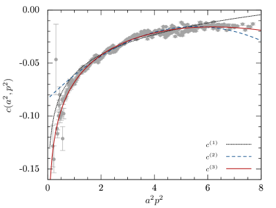
Figure 9: The expansion coefficient, $c(a^{2},p^{2})$, for the H4 term $a^{2}p^{[4]}/p^{2}$ in the expansion (22) and (24) of $Z(p)$. The data are for ensemble IV. The three lines refer to different fit ansatzes for the $a^{2}p^{2}$ dependence (see Eq. (27).)

In short, our analysis of the fitted H4 expansion seems to favor the functional form $c^{(3)}(a^{2},p^{2})$ which we adapted from 1-loop lattice perturbation theory. It better reproduces the observed behavior for large $a^{2}p^{2}$ and hence could improve global H4 fits, e.g., as performed in de Soto and Roiesnel (2007).

IV Summary

We have studied the quark propagator in Landau gauge on $N_{f}=2$ gauge field configurations using ${\cal O}(a)$-improved Wilson fermions for both large and almost physical quark masses.

In agreement with previous studies, we find that the quark wave function, $Z(p^{2})$, is infrared suppressed and the quark mass function, $M(p^{2})$, shows the same qualitative features as in previous studies with other discretizations, with a dynamically quark mass developing for momenta below 1–2 GeV, tending to a value $M(0)\approx 300$ MeV in the chiral limit. Compared to results using staggered and overlap fermions, $M(p^{2})$ drops more quickly when increasing $p$ from $200\,\text{MeV}$ to $p=1\,\text{GeV}$. We also do not see a clear sign of a plateau at small momenta. Lattice data below $p=200\,\text{MeV}$ are needed to determine whether such a plateau exists.

Our final lattice data for $M(p)$ are shown in the right panels of Figs. 4 and 4. These data were obtained applying the hybrid tree-level correction described above and restricting to cylinder-cut momenta. We tried to reduce the remaining hypercubic artifacts using the H4 method, but found that a linear extrapolation in $a^{2}p^{[4]}/p^{2}$ at fixed $p^{2}$ fails for $M(p)$. Higher hypercubic corrections terms are needed to reach at reasonable $\chi^{2}/d.o.f$ values. However, this introduces rather large uncertainties in the extrapolation, in particular a systematic error: at lower $ap$ ($ap=3\ldots 8$) the corrections come out to be significantly larger than at higher momenta ($ap>16$), where they are almost negligible. For $ap<3$ the H4 extrapolations gives no reasonable $\chi^{2}/d.o.f.$ values.

Our final results for $Z(p^{2})$ are shown in Fig. 8. There we show the results for cylinder-cut momenta after hybrid tree-level correction and our linear H4 extrapolation. This extrapolation has been successful for momenta above $p\simeq 1\,\text{GeV}$ and shifted the point where $Z$ starts to bend down to a larger $p^{2}$. Lattice spacing effects could not completely be eliminated but much reduced by applying those techniques. For large momenta, the wave function is essentially independent of quark mass and volume, while the infrared suppression at small momentum becomes stronger for smaller quark mass. We also find competing finite volume and lattice spacing effects at small $p$: the suppression becomes weaker with larger volumes, but stronger towards smaller lattice spacings.

Our study is the first to use fully dynamical ${\cal O}(a)$-improved Wilson fermions to access the quark wave and mass function. Lattice calculations, for example, of the nonperturbative RI’(S)MOM renormalization constants for hadron physics (see, e.g., Göckeler et al. (2010)), typically did not use those. We were able to reduce lattice spacing artifacts to percent level and at the same time studied a range of quark masses down to an almost physical value.

Appendix A On the Tree-Level Corrected Running Quark Mass

For the tree-level correction of the running quark mass data we used the hybrid prescription described in Section II.3 and Skullerud et al. (2001). We chose this because we found that it generally provides a smoother momentum dependence for $M$ than, for example, the multiplicative tree-level correction (see Section II.3 for a definition). To demonstrate the advantage of the hybrid correction we compare in Fig. 10 tree-level corrected data for the two prescriptions. We chose the lightest quark mass ensemble V for this. We see hat both corrections give comparable results (within one standard deviation) at low momenta ($ap<0.3$), but the multiplicatively corrected points deviate strongly from the hybrid corrected points in the mid-momentum regime ($0.3<ap<2$). At large $ap$ the two curves seem to approach each other again, but still at $p=8.6$ GeV, the highest momenta accessible in our study, the two $M$’s differ by many standard deviations: for the multiplicatively corrected quark mass function we have $M(8.6\,\text{GeV})=3.1176\pm 0.0019\,\text{MeV}$, while for the hybrid corrected mass function we have $M(8.6\,\text{GeV})=2.602\pm 0.0094\,\text{MeV}$.

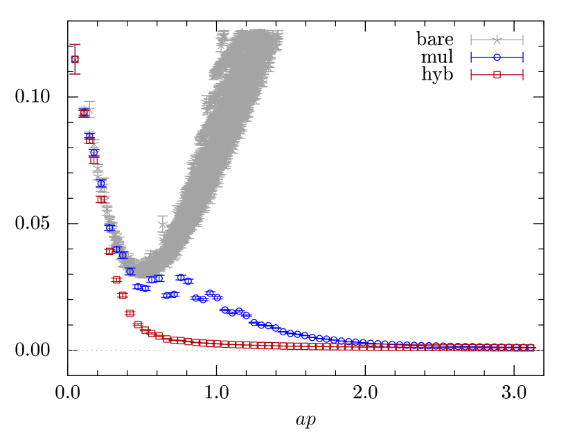
Figure 10: Hybrid and multiplicatively tree-level corrected mass function $aM(p)$ versus the uncorrected data for ensemble V as a function of $ap$. The momenta for the corrected data have been cylinder cut with a radius of 1 lattice momentum unit. The uncorrected data have not been cut.

A more detailed investigation of the multiplicatively corrected mass function in the mid-momentum regime shows that it is the lattice momenta along the diagonal which deviate most strongly from the general trend in the data. This somewhat surprising result can be understood looking again at Fig. 2: For diagonal momenta, the mass function $aM_{\mathrm{rot}}^{(0)}(p)=am+a\Delta M_{\mathrm{rot}}^{(0)}(p)$ is very close to $am$ but stays below $am$ within $0\leq a^{2}p^{2}\leq 4$. For on-axis momenta, on the other hand $aM_{\mathrm{rot}}^{(0)}(p)$ rises fast with $a^{2}p^{2}$. The smallness of $aM_{\mathrm{rot}}^{(0)}(p)$ for diagonal momenta $0\leq a^{2}p^{2}\leq 4$ results in small values for $Z_{m}=aM_{\mathrm{rot}}^{(0)}(p)/am$. Applying $Z_{m}$ artificially enhances the multiplicatively corrected $M=M_{L}/Z_{m}$, which may even become negative for very small $am$. The hybrid correction does not have this feature, and provides a smooth curve for $M$ for all momenta.

References

- Roberts and Williams (1994) Craig D. Roberts and Anthony G. Williams, “Dyson-Schwinger equations and their application to hadronic physics,” Prog. Part. Nucl. Phys. 33, 477–575 (1994), arXiv:hep-ph/9403224 [hep-ph] .
- Fischer (2006) Christian S. Fischer, “Infrared properties of QCD from Dyson-Schwinger equations,” J. Phys. G32, R253–R291 (2006), arXiv:hep-ph/0605173 [hep-ph] .
- Cloet and Roberts (2014) Ian C. Cloet and Craig D. Roberts, “Explanation and Prediction of Observables using Continuum Strong QCD,” Prog. Part. Nucl. Phys. 77, 1–69 (2014), arXiv:1310.2651 [nucl-th] .
- Eichmann et al. (2016) Gernot Eichmann, Helios Sanchis-Alepuz, Richard Williams, Reinhard Alkofer, and Christian S. Fischer, “Baryons as relativistic three-quark bound states,” Prog. Part. Nucl. Phys. 91, 1–100 (2016), arXiv:1606.09602 [hep-ph] .
- Williams (2015) Richard Williams, “The quark-gluon vertex in Landau gauge bound-state studies,” Eur. Phys. J. A51, 57 (2015), arXiv:1404.2545 [hep-ph] .
- Williams et al. (2016) Richard Williams, Christian S. Fischer, and Walter Heupel, “Light mesons in QCD and unquenching effects from the 3PI effective action,” Phys. Rev. D93, 034026 (2016), arXiv:1512.00455 [hep-ph] .
- Cyrol et al. (2018) Anton K. Cyrol, Mario Mitter, Jan M. Pawlowski, and Nils Strodthoff, “Nonperturbative quark, gluon, and meson correlators of unquenched QCD,” Phys. Rev. D97, 054006 (2018), arXiv:1706.06326 [hep-ph] .
- Aguilar et al. (2018) A. C. Aguilar, J. C. Cardona, M. N. Ferreira, and J. Papavassiliou, “Quark gap equation with non-abelian Ball-Chiu vertex,” Phys. Rev. D98, 014002 (2018), arXiv:1804.04229 [hep-ph] .
- Becirevic et al. (2000a) D. Becirevic, V. Lubicz, G. Martinelli, and M. Testa, “Quark masses and renormalization constants from quark propagator and three point functions,” Nucl. Phys. Proc. Suppl. 83, 863–865 (2000a), arXiv:hep-lat/9909039 [hep-lat] .
- Becirevic et al. (2000b) Damir Becirevic, Vicente Gímenez, Vittorio Lubicz, and Guido Martinelli, “Light quark masses from lattice quark propagators at large momenta,” Phys. Rev. D61, 114507 (2000b), arXiv:hep-lat/9909082 [hep-lat] .
- Skullerud and Williams (2001) Jon Ivar Skullerud and Anthony G. Williams, “Quark propagator in Landau gauge,” Phys. Rev. D63, 054508 (2001), arXiv:hep-lat/0007028 [hep-lat] .
- Skullerud et al. (2001) Jonivar Skullerud, Derek B. Leinweber, and Anthony G. Williams, “Nonperturbative improvement and tree level correction of the quark propagator,” Phys. Rev. D64, 074508 (2001), arXiv:hep-lat/0102013 [hep-lat] .
- Boucaud et al. (2003) Philippe Boucaud, F. de Soto, J. P. Leroy, A. Le Yaouanc, J. Micheli, H. Moutarde, O. Pè ne, and J. Rodríguez-Quintero, “Quark propagator and vertex: Systematic corrections of hypercubic artifacts from lattice simulations,” Phys. Lett. B575, 256–267 (2003), arXiv:hep-lat/0307026 [hep-lat] .
- Bowman et al. (2002) Patrick O. Bowman, Urs M. Heller, and Anthony G. Williams, “Lattice quark propagator with staggered quarks in Landau and Laplacian gauges,” Phys. Rev. D66, 014505 (2002), arXiv:hep-lat/0203001 [hep-lat] .
- Parappilly et al. (2006) Maria B. Parappilly, Patrick O. Bowman, Urs M. Heller, Derek B. Leinweber, Anthony G. Williams, and J. B Zhang, “Scaling behavior of quark propagator in full QCD,” Phys. Rev. D73, 054504 (2006), arXiv:hep-lat/0511007 [hep-lat] .
- Bowman et al. (2005) Patrick O. Bowman, Urs M. Heller, Derek B. Leinweber, Maria B. Parappilly, Anthony G. Williams, and Jian-Bo Zhang, “Unquenched quark propagator in Landau gauge,” Phys. Rev. D71, 054507 (2005), arXiv:hep-lat/0501019 [hep-lat] .
- Furui and Nakajima (2005) Sadataka Furui and Hideo Nakajima, “Unqueched Kogut-Susskind quark propagator in lattice Landau gauge QCD,” (2005), arXiv:hep-lat/0511045 [hep-lat] .
- Bonnet et al. (2002) Frederic D. R. Bonnet, Patrick O. Bowman, Derek B. Leinweber, Anthony G. Williams, and Jian-Bo Zhang (CSSM Lattice), “Overlap quark propagator in Landau gauge,” Phys. Rev. D65, 114503 (2002), arXiv:hep-lat/0202003 [hep-lat] .
- Zhang et al. (2004) J. B. Zhang, Patrick O. Bowman, Derek B. Leinweber, Anthony G. Williams, and Frederic D. R. Bonnet (CSSM Lattice), “Scaling behavior of the overlap quark propagator in Landau gauge,” Phys. Rev. D70, 034505 (2004), arXiv:hep-lat/0301018 [hep-lat] .
- Zhang et al. (2005) J. B. Zhang, Patrick O. Bowman, Ryan J. Coad, Urs M. Heller, Derek B. Leinweber, and Anthony G. Williams, “Quark propagator in Landau and Laplacian gauges with overlap fermions,” Phys. Rev. D71, 014501 (2005), arXiv:hep-lat/0410045 [hep-lat] .
- Kamleh et al. (2005) Waseem Kamleh, Patrick O. Bowman, Derek B. Leinweber, Anthony G. Williams, and Jianbo Zhang, “The fat link irrelevant clover overlap quark propagator,” Phys. Rev. D71, 094507 (2005), arXiv:hep-lat/0412022 [hep-lat] .
- Kamleh et al. (2007) Waseem Kamleh, Patrick O. Bowman, Derek B. Leinweber, Anthony G. Williams, and Jianbo Zhang, “Unquenching effects in the quark and gluon propagator,” Phys. Rev. D76, 094501 (2007), arXiv:0705.4129 [hep-lat] .
- Schröck (2012) Mario Schröck, “The chirally improved quark propagator and restoration of chiral symmetry,” Phys. Lett. B711, 217–224 (2012), arXiv:1112.5107 [hep-lat] .
- Blossier et al. (2011) B. Blossier, Ph. Boucaud, M. Brinet, F. De Soto, Z. Liu, V. Morenas, O. Pène, K. Petrov, and J. Rodríguez-Quintero, “Renormalisation of quark propagators from twisted-mass lattice QCD at =2,” Phys. Rev. D83, 074506 (2011), arXiv:1011.2414 [hep-ph] .
- Burger et al. (2013) Florian Burger et al., “Quark mass and chiral condensate from the Wilson twisted mass lattice quark propagator,” Phys. Rev. D87, 034514 (2013), [Phys. Rev.D87,079904(2013)], arXiv:1210.0838 [hep-lat] .
- August and Maas (2013) Daniel August and Axel Maas, “On the Landau-gauge adjoint quark propagator,” JHEP 07, 001 (2013), arXiv:1304.4423 [hep-lat] .
- Oliveira et al. (2016) Orlando Oliveira, Ayşe Kızılersü, Paulo J. Silva, Jon-Ivar Skullerud, Andre Sternbeck, and Anthony G. Williams, “Lattice Landau gauge quark propagator and the quark-gluon vertex,” Proceedings, International Meeting Excited QCD 2016, Acta Phys. Polon. Supp. 9, 363–368 (2016), arXiv:1605.09632 [hep-lat] .
- Bali et al. (2013) G. S. Bali et al., “Nucleon mass and sigma term from lattice QCD with two light fermion flavors,” Nucl. Phys. B866, 1–25 (2013), arXiv:1206.7034 [hep-lat] .
- Bali et al. (2014) Gunnar S. Bali et al., “The moment of the nucleon from lattice QCD down to nearly physical quark masses,” Phys. Rev. D90, 074510 (2014), arXiv:1408.6850 [hep-lat] .
- Bali et al. (2015) Gunnar S. Bali et al., Phys. Rev. D91, 054501 (2015), arXiv:1412.7336 [hep-lat] .
- Sheikholeslami and Wohlert (1985) B. Sheikholeslami and R. Wohlert, “Improved Continuum Limit Lattice Action for QCD with Wilson Fermions,” Nucl. Phys. B259, 572 (1985).
- Heatlie et al. (1991) G. Heatlie, G. Martinelli, C. Pittori, G. C. Rossi, and Christopher T. Sachrajda, “The improvement of hadronic matrix elements in lattice QCD,” Nucl. Phys. B352, 266–288 (1991).
- Pennington (2005) M. R. Pennington, “Swimming with quarks,” Particles and fields. Proceedings, 11th Mexican School, Xalapa, Veracruz, Mexico, August 2-13, 2004, J. Phys. Conf. Ser. 18, 1–73 (2005), arXiv:hep-ph/0504262 [hep-ph] .
- Leinweber et al. (1999) Derek B. Leinweber, Jon Ivar Skullerud, Anthony G. Williams, and Claudio Parrinello (UKQCD), “Asymptotic scaling and infrared behavior of the gluon propagator,” Phys. Rev. D60, 094507 (1999), [Erratum: Phys. Rev.D61,079901(2000)], arXiv:hep-lat/9811027 [hep-lat] .
- Becirevic et al. (1999) D. Becirevic, Philippe Boucaud, J. P. Leroy, J. Micheli, O. Pène, J. Rodríguez-Quintero, and C. Roiesnel, “Asymptotic behavior of the gluon propagator from lattice QCD,” Phys. Rev. D60, 094509 (1999), arXiv:hep-ph/9903364 [hep-ph] .
- de Soto and Roiesnel (2007) F. de Soto and C. Roiesnel, “On the reduction of hypercubic lattice artifacts,” JHEP 09, 007 (2007), arXiv:0705.3523 [hep-lat] .
- Fischer and Alkofer (2003) Christian S. Fischer and Reinhard Alkofer, “Nonperturbative propagators, running coupling and dynamical quark mass of Landau gauge QCD,” Phys. Rev. D67, 094020 (2003), arXiv:hep-ph/0301094 [hep-ph] .
- Aguilar and Papavassiliou (2011) A. C. Aguilar and J. Papavassiliou, “Chiral symmetry breaking with lattice propagators,” Phys. Rev. D83, 014013 (2011), arXiv:1010.5815 [hep-ph] .
- Constantinou et al. (2009) M. Constantinou, V. Lubicz, H. Panagopoulos, and F. Stylianou, “ corrections to the one-loop propagator and bilinears of clover fermions with Symanzik improved gluons,” JHEP 10, 064 (2009), arXiv:0907.0381 [hep-lat] .
- Göckeler et al. (2010) M. Göckeler et al., “Perturbative and Nonperturbative Renormalization in Lattice QCD,” Phys. Rev. D82, 114511 (2010), [Erratum: Phys. Rev.D86,099903(2012)], arXiv:1003.5756 [hep-lat] .