Random walk on temporal networks with lasting edges

Abstract

We consider random walks on dynamical networks where edges appear and disappear during finite time intervals. The process is grounded on three independent stochastic processes determining the walker’s waiting-time, the up-time and down-time of edges activation. We first propose a comprehensive analytical and numerical treatment on directed acyclic graphs. Once cycles are allowed in the network, non-Markovian trajectories may emerge, remarkably even if the walker and the evolution of the network edges are governed by memoryless Poisson processes. We then introduce a general analytical framework to characterize such non-Markovian walks and validate our findings with numerical simulations.

I Introduction

Random walks play a central role in different fields of science [1, 2, 3]. Despite the apparent simplicity of the process, the study of random walks remains an active domain of research [4, 5, 6, 7, 8]. Within the field of network science, a central theme focuses on the relation between patterns of diffusion and network structure [9]. Important applications include the design of centrality measures based on the density of walkers on nodes [10], or community detection methods looking for regions of the network where a walker remains trapped for long times [11, 12, 13]. The mathematical properties of random walks on static networks are overall well-established [14], and essentially equivalent to those of a Markov chain. However, the process becomes much more challenging when the network is itself a dynamical entity, with edges appearing and disappearing in the course of time [15, 16, 17]. The temporal properties of networks have been observed and studied in a variety of empirical systems, and their impact on diffusive processes explored by means of numerical simulations [18, 19, 20] and analytical tools [21].

Mathematical analysis of dynamics on temporal networks often relies on the assumption that links activate during an infinitesimal duration [22]. In the case of random walks, this framework naturally reduces to standard continuous-time random walk on static, weighted networks. Even in this simplified case, however, the dynamics exhibits interesting properties including the so-called waiting-time paradox. When the dynamics of the edges is Poissonian, trajectories are encoded by a Markov chain, whereas the timings obtained from a non-Poisson renewal process lead to non-trivial properties such as the emergence of non-Markovian trajectories. In that case the trajectory of the walker generally depends on its previous trajectory and not only on its current location [23, 24]. The emergence of non-Markovian trajectories is even more pronounced in situations when the activations of edges are correlated, often requiring the use of higher-order models for the data [25, 26]. However, this whole stream of research neglects an important aspect on the edge dynamics, the non-zero duration of their activation, which has been observed and characterised in a variety of real-life systems, including sensor data [27, 28, 29]. The finite duration of edges availability has important practical implications, including in community detection [30]. Theoretically, some results have been obtained within the framework of switching systems, e.g. by replacing the constant laplacian matrix $L$ by a time-dependent one $L(t)$ for the diffusion [31, 32, 33], but a master equation approach derived from a microscopic model of the dynamics is, to the best of our knowledge, still lacking.

Our main objective is to develop an analytical framework for random walks on temporal networks with finite activation times. Given a network of potential connections between a fixed set of nodes, the model is defined by three temporal processes. Each process comes with its own timescale, associated to the motion of the random walker, the duration between two successive activations of the edges and the duration of these activations. In contrast with previous research, we derive a master equation from the model specifications, without implicitly assuming memoryless dynamics for the walker, and consider the resulting trajectories of the random walker [34]. The competition between three timescales makes the problem particularly rich and we show how certain master equations already known in the literature are recovered in limit regimes.

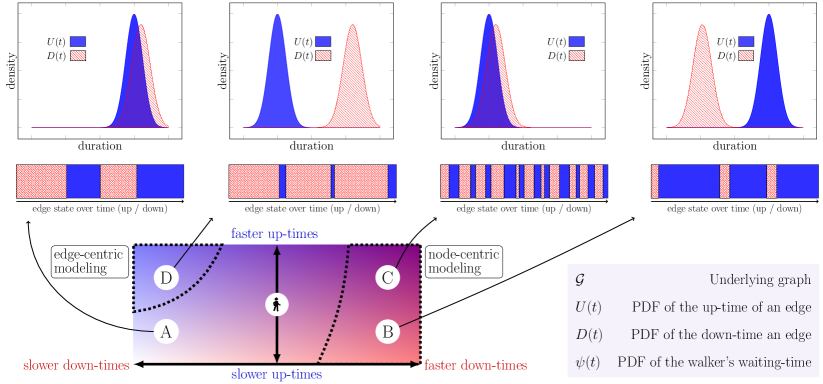
Figure 1: Three timescales are present in the model : one governing the rest state of the walker in the nodes and two associated with the activation and deactivation of the edges. The overall dynamics will depend on the relative weights of such timescales, as we schematically report here. The bottom panel represents the up-time and down-time durations of the edges with respect to the walker’s self-imposed waiting-time upon arrival on a node. The four corners identified by the letters $A$ to $D$ represent the cases where the timescale for the edges’ dynamics is clearly separated from that of the walker (hereby located in the center of the domain of the bottom panel, and schematically represented by a standing icon). Each of these four situations is described by one of the four top panels, representing typical up-time and down-time probability density functions (PDF’s) $U(t)$ and $D(t)$, which complement the walker’s possibly node-dependent PDF $\psi(t)$ as the three dynamical parameters of the model. The rectangles with the red and blue bars show representative realizations of the stochastic processes of edge activation and deactivation according to the densities reported above. The blue shaded (resp. red hatched) rectangles stand for periods of edge availability (resp. unavailability). The proposed model depends on the four parameters in the bottom right panel. It is general enough to tackle also the situations where there is no sharp timescale separation, and none of the dynamics is extreme enough to be neglected, as in the region bounded by the dashed lines in the bottom panel.

This paper is organised as follows. In section II, we describe the model and its parameters. In section III, we derive a master equation for the density of the walker valid for directed acyclic graphs (DAGs). Particular cases for the model parameters and their ensuing dynamics are discussed. These equations are revisited in section IV, where we consider the impact of cycles in the graph on the Markovianity of the process. The analytical predictions are confronted with numerical simulations throughout this work. Section V gives more details about the numerical implementation of our formalism. We finally conclude and give perspectives in section VI.

II The model

Let $V$ be a fixed set of $N$ nodes and $E$ be a set of directed edges between these nodes. We denote by $\mathcal{G}=(V,E)$ the static graph determining which edges are available in the dynamic graph with time-dependent adjacency matrix $A(t)$. The dynamic graph can assume any of the $2^{\left|E\right|}$ possible configurations allowed by $\mathcal{G}$. In our model-driven approach, each edge $(i,j)=i\rightarrow j\in E$ is characterized by

• a down-time probability density function (PDF) $D_{ij}(t)$, $t\in\mathbb{R}^{+}$, which determines for how long the edge remain inactive;

• an up-time PDF $U_{ij}(t)$, $t\in\mathbb{R}^{+}$, which rules the duration that the edge is available to the walker.

In this work, the random variables associated with the densities $U_{ij}$ and $D_{ij}$ are assumed to have finite expectation. The adjacency matrix can be written as

$$A(t)=\sum\limits_{i\in\mathbb{Z}}G_{i}\mathbbm{1}_{\{t_{i}\leq t<t_{i+1}\}}(t)$$ (1)

with $\ldots<t_{-1}<t_{0}\leq 0<t_{1}<\ldots$ the successive times of the rewiring, and $G_{i}$ a fixed adjacency matrix (figure 2). Let $k_{i}^{\rm in}(t)=\sum_{j=1}^{N}A_{ji}(t)$ be the in-degree of node $i$ at time $t$, and $k_{i}^{\rm out}(t)=\sum_{j=1}^{N}A_{ij}(t)$ be the out-degree. We define the set of nodes reachable from $i$ in the underlying graph $V_{i}=\left\{j\in V\ |\ i\rightarrow j\in E\right\}$, and $|V_{i}|$ its cardinality, namely the out-degree of node $i$ in $\mathcal{G}$. Similarly, $V^{\prime}_{i}=\left\{j\in V\ |\ j\rightarrow i\in E\right\}$ and $|V^{\prime}_{i}|$ results to be the in-degree of node $i$. We make the assumption that there are no isolated nodes in $\mathcal{G}$ : for every $i\in E$, $\max\{|V_{i}|,|V^{\prime}_{i}|\}>0$.

Let us define the random walk. A continuous-time random walk on a dynamical graph with adjacency matrix $A(t)$, $t\in\mathbb{R}$ is a process $\left\{A(t),{i}_{W}(t)\right\}$ where ${i}_{W}(t)\in V$ is the node occupied by the walker at time $t$. Upon arrival on a node $i$, the walker is assigned a waiting-time according to the PDF $\psi_{i}(t)$ which generally depends on the node (see Fig. 2, first, second and third cartoon from the left). After the waiting-time has elapsed, the walker selects one of the available leaving edges uniformly, namely with probability $1/k_{i}^{\rm out}(t)$. If no edge is available, the walker is trapped on the node (Fig. 2, fourth cartoon) and waits for the first leaving edge to appear to perform the jump (Fig. 2, fifth cartoon). Note that in the latter case, almost surely there is no choice to be made there : no two or more edges can activate at the same time.

Let us observe that a possible variant of this random walk could consist in assigning a new waiting-time according to $\psi_{i}$ for the walker trapped on a node because of the lack of available edges once it is ready to jump. This process was studied in [34], where the authors exclusively focus on the asymptotic state of the process.

Our model is an extension of the standard active node-centric and passive edge-centric random walks in temporal networks [17], where edge duration is instantaneous. In the former, the motion is determined by the waiting-time of the walker and, once a jump takes place, all the edges in $\mathcal{G}$ are available - or at least the ones exiting from the node where the walker is located. In the latter case, the walker is ready to jump as soon as it arrives on a new node, and it takes the first edge that appears - the walker thus passively follows the appearing edges modeled by a renewal process. These two cases correspond to asymptotic regimes described by our model when a timescale dominates over the others. In general, however, the process is determined by the competition of three timescales. Figure 1 summarizes possible scenarios labeled from $A$ to $D$ corresponding to the four distinct cases, where the dynamics of the down- and up-times are either significantly faster or significantly slower than the characteristic waiting-time of the walker. At the right border of the domain, in the region ranging from $B$ to $C$, when the walker is ready to jump the possible extra waiting-time for an edge to become available is usually short, and the network dynamics can be neglected. Therefore, the node-centric random walk is a good proxy for our model. In the region centered around $D$, the same type of analysis leads instead to neglecting the waiting-time of the walker. In general however, as in the center of the domain, in the area between the dotted regions, neither the walker nor the edges dynamics can be neglected. This region is the focus of our work.

Figure 2: Directed temporal network with four nodes (below) and the (1,3) entry of the time-dependent adjacency matrix $A(t)$ (above). Note that $A(t)$ is right-continuous and is given by $A(t)=G_{i}$ for $t_{i}\leq t<t_{i+1}$. In this example, the up-time $t_{m+2}-t_{m+1}$ of edge $1\rightarrow 3$ follows the density $U_{13}(t)$, while the down-time $t_{m+4}-t_{m+2}$ has density $D_{13}(t)$. At every random rewiring time $t_{i}$, almost surely only one edge changes.

III The case of directed acyclic graphs

As a first step, we consider the trajectory of a walker performing a random walk as defined above on a directed acyclic graph (DAG). The reason for that is twofold.

1. DAGs include directed trees and find many applications, see for instance [35]. Every undirected graph possesses an acyclic orientation. Moreover, by contracting each strongly connected component, every directed graph can be mapped to a DAG. Figure 3 illustrates that process. The material presented in this section therefore provides tools to analyse a random walk on a coarse grained model obtained by condensation of a given graph into a DAG.

2. As we will show next, the presence of cycles in the graph will remove the Markov property from the random walk. Hence, the analysis of our model on a DAG will serve, in a second step, as a limiting case on which to consider more general organizations. The approximation using DAGs is expected to be good when edges along a path can be considered statistically independent. The conditions for this to hold will be discussed further in section IV.

As will become clear (see III.5), the model on DAGs can be viewed as a one-density, node-centric (or edge-centric) random walk.

Figure 3: Mapping of a directed network with cycles (top) to a DAG (bottom) through a condensation process. Strongly connected components are transformed into super-nodes.

III.1 The master equation on a DAG

The notations in this section are adapted from [22]. Let $n_{i}(t)$ be the probability for the walker to be on node $i$ at time $t$,

$$n_{i}(t)=\rm P\{i_{W}(t)=i\}.$$ (2)

If $q_{i}(t)$ is the PDF of the arrival time on node $i$, and $\Phi_{i}(t,\tau)$ is to probability to stay on node $i$ on the interval $[\tau,t]$ with $\tau$ the arrival time on node $i$, then

$$n_{i}(t)=\int_{0}^{t}q_{i}(\tau)\Phi_{i}(t,\tau)\rm d\tau.$$ (3)

Let $T_{ji}(t,\tau)$ be the PDF of the transition time from node $i$ to $j$, with $\tau$ the arrival time on node $i$. Let also $T_{\bullet i}(t,\tau)$ denote the PDF of the time of the jump from node $i$. We have

$$\Phi_{i}(t,\tau) =1-\int_{\tau}^{t}T_{\bullet i}(\nu,\tau)\rm d\nu$$

$$=1-\int_{\tau}^{t}\sum_{j\in V_{i}}T_{ji}(\nu,\tau)\rm d\nu.$$ (4)

We want to write the column vector ${\bf n}(t)=(n_{1}(t),\ldots,n_{N}(t))^{T}$ in terms of the transition density $T_{ij}$ and of the initial condition ${\bf n}(0)$. Looking at (3) and (4), we search for an appropriate expression for $q_{i}(t)$. Let $q_{i}^{(k)}(t)$ be the probability to arrive on node $i$ at time $t$ in exactly $k\in\mathbb{N}$ jumps. Then we have

$$q_{i}(t)=\sum\limits_{k=0}^{\infty}q_{i}^{(k)}(t)=\sum\limits_{k\geq 1}q_{i}^{(k)}(t)+q_{i}^{(0)}(t),$$ (5)

with initial condition $q_{i}^{(0)}(t)=n_{i}(0)\delta(t)$. Equivalently,

$$q_{i}(t)=\sum\limits_{k=0}^{\infty}q_{i}^{(k+1)}(t)+q_{i}^{(0)}(t),$$ (6)

where

$$q_{i}^{(k+1)}(t)=\sum_{j}\int_{0}^{t}q_{j}^{(k)}(\nu)T_{ij}(t,\nu)\rm d\nu.$$ (7)

Summing on both sides over $k\geq 0$ and adding $q_{i}^{(0)}(t)$ yields

$$q_{i}(t)=\sum_{j}\int_{0}^{t}q_{j}(\nu)T_{ij}(t,\nu){\rm d}\nu+q_{i}^{(0)}(t).$$ (8)

In vector form, with $\mathbf{q}(t)=\left(q_{1}(t),\ldots,q_{N}(t)\right)^{T}$, we have

$$\mathbf{q}(t)=\mathcal{T}\mathbf{q}(t)+\mathbf{q}^{(0)}(t)$$ (9)

where $\mathcal{T}$ is the linear integral operator acting on $\mathbf{q}(t)$ defined by :

$$\mathcal{T}\mathbf{q}(t)=\int_{0}^{t}T(t,\nu)\mathbf{q}(\nu)\mathrm{d}\nu,\quad i=1,\ldots,N$$ (10)

where $T(t,\nu)$ is a matrix function with component $(i,j)$ given by $T_{ij}(t,\nu)$. Due to the acyclic nature of the graph and as will become clear after remark 3 at the end of section III.3, the transition density actually only depends on the duration $t-\tau$. As a result, equation (10) is a convolution and applying a Laplace transform allows to solve (9) for $\mathbf{q}(t)$, as was done in [22].

Once $\mathbf{q}(t)$ is found, we consider equation (3), which can be cast under the form

$$\mathbf{n}(t)=\mathcal{P}\mathbf{q}(t)$$ (11)

where operator $\mathcal{P}$ is diagonal and given by

$$\left(\mathcal{P}\mathbf{q}(t)\right)_{i}=\int_{0}^{t}\Phi_{i}(t,\tau)q_{i}(\tau)\mathrm{d}\tau,\quad i=1,\dots,N.$$ (12)

Observe that this is again a convolution, because $\Phi_{i}(t,\tau)$ is essentially $\Phi_{i}(t-\tau)$. The right-hand-side of (12) can be computed directly in the time-domain, or through a Laplace transform. In the latter case we obtain for each component $\hat{{n}}_{i}(s):=\int_{0}^{\infty}n_{i}(t)e^{-st}\mathrm{d}t$ a product in the Laplace domain, and we ultimately find $\mathbf{n}(t)=(n_{1}(t),\ldots,n_{N}(t))$ as a function of the initial density $\mathbf{n}(0)$ by computing the inverse transform of these products.

III.2 On the use of the Laplace transform in the case of a DAG

It is not mandatory to use the Laplace transform to solve the integral equations $\mathbf{q}(t)$ and then get $\mathbf{n}(t)$. We can proceed directly in the time domain and solve the equation relying on the acyclic nature of the graph. We detail this alternative approach, which does not rely on the convolution structure of the integral equations.

Remark 1.

This method also applies when we drop the acyclic assumption on $\mathcal{G}$ in section IV and we have to solve equation (50).

Let us first recall Neumann’s Lemma.

Theorem 1.

Let $\mathcal{T}$ be a linear bounded operator on a Banach space $X$. If $||\mathcal{T}||=\sup_{||x||\leq 1}||\mathcal{T}x||<1$, then $I-\mathcal{T}$ is invertible and is given by the Neumann series

$$(I-\mathcal{T})^{-1}=\sum_{k=0}^{\infty}T^{k}=I+\mathcal{T}+\mathcal{T}^{2}+\ldots.$$

The theorem is applicable for this convolution-type linear Volterra integral equation with square integrable convolution kernels (see [36] theorem 3.7.7 page 77), and equation (9) gives

$$\mathbf{q}(t) =(I-\mathcal{T})^{-1}\mathbf{q}^{(0)}(t)$$

$$=\sum_{k=0}^{\infty}\mathcal{T}^{k}\mathbf{q}^{(0)}(t)$$ (13)

$$=\sum_{k=0}^{\infty}\mathcal{T}^{k}\delta(t)\mathbf{n}{(0)}.$$ (14)

If we compute the iterates of $\mathcal{T}$ acting on $\mathbf{q}^{(0)}(t)$, we see that the successive terms $\mathcal{T}^{k}\mathbf{q}^{(0)}(t)$, with $\mathbf{q}^{(0)}(t)=\mathbf{n}^{(0)}\delta(t)$, account for the probability to arrive on a given node at time $t$, starting from the initial condition $\mathbf{n}^{(0)}$, in exactly $k$ steps.

Remark 2.

In general, the Neumann series does not offer a practical way for computing $(I-\mathcal{T})^{-1}$ since it involves an infinite number of terms. Because we make the assumption that the underlying graph $\mathcal{G}$ has no cycles, the series can be cut after $d$ terms, where $d$ is the diameter of the graph.

Based on (3) we can now compute $\dot{\mathbf{n}}(t)$ in terms of the transition density and of the initial conditions. Applying Leibniz’s rule for differentiation under the integral sign, we obtain

$${\dot{n}_{i}}(t) =q_{i}(t)-\int_{0}^{t}q_{i}(\tau)\sum_{j\in V_{i}}T_{ji}(t,\tau)\mathrm{d}\tau$$

$$=q_{i}(t)-\int_{0}^{t}q_{i}(\tau)T_{\bullet i}(t,\tau)\mathrm{d}\tau.$$ (15)

The interpretation is that the rate of evolution of $n_{i}(t)$ is given by a sum of all arrivals minus the departures, with each departure resulting from a previous arrival at any point in time. Let us define a diagonal integral operator $\mathcal{D}$ acting on $\mathbf{q}$ by its $i$-th component :

$$\left(\mathcal{D}\mathbf{q}(t)\right)_{i}=\int_{0}^{t}T_{\bullet i}(t,\tau)q_{i}(\tau)\mathrm{d}\tau.$$ (16)

Equation (15) can now be written as

$$\dot{\mathbf{n}}(t) =(I-\mathcal{D})\mathbf{q}(t)$$

$$=(I-\mathcal{D})\sum_{k=0}^{\infty}\mathcal{T}^{k}\mathbf{q}^{(0)}(t)$$ (17)

where we have used (13) to obtain the second equation.

III.3 Transition density on DAGs

The equation for $\mathbf{n}(t)$ remains abstract unless we can write $T_{ji}$ explicitly in terms of the model parameters contained in figure 1. For the sake of simplicity and without lack of generality in the reasoning, we assume that all edges share the same up-time and down-time densities : $U_{ij}(t)=:U(t)$ and $D_{ij}(t)=:D(t)$, for all $i,j=1,\ldots,N$.

Let $p$ denote the probability that a given edge of $\mathcal{G}$ is active (up-state) at a random time. Recall that we assume up-time and down-time durations with finite expectation. It results that

$$p=\mathrm{P}\left\{\mathrm{edge\ }i\rightarrow j\ \mbox{is active}\right\}=\frac{\langle U\rangle}{\langle U\rangle+\langle D\rangle}$$ (18)

where $\langle f\rangle=\int_{\mathbb{R}}tf(t)\mathrm{d}t$ is the mathematical expectation of the random variable with PDF $f(t)$. We decompose the transition density in two terms : $T_{ji}(t,\tau)=(\mathbf{1})+(\mathbf{2})$. The first term corresponds to the case that an edge is available to the jumper at the end of his waiting-time:

$$(\mathbf{1})=\psi_{i}(t-\tau)\sum_{k=1}^{|V_{i}|}\frac{1}{k}\binom{|V_{i}|-1}{k-1}p^{k}(1-p)^{|V_{i}|-k}.$$ (19)

Edge $i\rightarrow j$ has to be available, and needs to be chosen amongst the $|V_{i}|-1$ other edges which are also active at time $t$. A straightforward computation allows to rewrite equation (19) as

$$(\mathbf{1})=\psi_{i}(t-\tau)\frac{1}{|V_{i}|}\left[1-(1-p)^{|V_{i}|}\right].$$ (20)

The quantity between square brackets is the probability that at least one edge is available. The factor $1/|V_{i}|$ appears because all outgoing edges are treated indifferently, and so the probability to be chosen is distributed uniformly amongst all edges including $i\rightarrow j$.

In the second case represented by figure 4, the jump occurs after the walker happened to be trapped. Let us observe that when the walker becomes trapped on node $i$, then for a given $j\in V_{i}$ the time $w$ before $i\rightarrow j$ becomes available has the PDF

$$\mathscr{D}(t)=\frac{1}{\langle D\rangle}\int_{t}^{\infty}D(\nu)\mathrm{d}\nu$$ (21)

as follows from the so-called bus-paradox.

Figure 4: Waiting-time $w$ of the trapped walker on node $i$, before activation of edge $i\rightarrow j$. The walker arrived at time $\tau$ on node $i$. After a waiting-time determined by the density $\psi_{i}(t)$, a jump can be performed but none of the $|V_{i}|$ outgoing edges is active. The walker needs to wait a subsequent duration $w$ before a link - here to node $j$- becomes available. So eventually the jump is performed at time $t$.

Edge $i\rightarrow j$ is selected by the trapped walker to perform the jump a time $t$ if $(i)$ the waiting-time expires before $t$, $(ii)$ at that moment all other edges are not active and will remain inactive at least until $t$, and $(iii)$ edge $i\rightarrow j$ was also down but becomes active exactly at time $t$. It results that

$$(\mathbf{2})=\int_{\tau}^{t}\psi_{i}(x-\tau)\big{[}(1-p)\mathrm{P}\left\{w>t-x\right\}\big{]}^{|V_{i}|-1}\\ \times(1-p)\mathscr{D}(t-x)\mathrm{d}x\\$$ (22)

or in a slightly more compact way,

$$(\mathbf{2})=(1-p)^{|V_{i}|}\int_{\tau}^{t}\psi_{i}(x-\tau)\mathscr{D}(t-x)\\ \times\big{[}\mathrm{P}\left\{w>t-x\right\}\big{]}^{|V_{i}|-1}\mathrm{d}x\\$$ (23)

where

$$\mathrm{P}\left\{w>t-x\right\}=\int_{t-x}^{\infty}\mathscr{D}(s)\mathrm{d}s.$$ (24)

In short, we have shown that

$$T_{ji}(t,\tau)=c_{1}\psi_{i}(t-\tau)\\ +c_{2}\int_{\tau}^{t}\psi_{i}(x-\tau)\left[\int_{t-x}^{\infty}\mathscr{D}(s)\mathrm{d}s\right]^{|V_{i}|-1}\mathscr{D}(t-x)\mathrm{d}x,$$ (25)

where $c_{1}$ and $c_{2}$ depend only on $\langle U\rangle$, $\langle D\rangle$, and $|V_{i}|$. For the sake of readability, we have dropped the index $i$ due to the node-dependence of $c_{1}$ and $c_{2}$. Observe that the distribution of $U$ only matters through its mean, because only the mean value $\langle U\rangle$ influences the probability $p$. On the other hand, if the walker is ready to jump during a down-time, then the jumps occur directly at the end of this down-time, and so the full distribution of $D$ does matter.

Remark 3.

Having assumed an acyclic directed network allows us to consider all outgoing edges the same way. There is no possibility for the walker to backtrack to its previous step. The time when an edge becomes available to the walker does not depend on the arrival time of the walker on the node, and the density $\mathscr{D}$ of $w$ can be applied for all outgoing edges. Indeed, if on the contrary the walker could jump across the cycle $i\rightarrow j\rightarrow i$, the probability for link $i\rightarrow j$ to still last can be large. This would induce a bias on the next jump, giving it more chance to end up again in $j$. It results that, as stated before, $T_{ji}(t,\tau)$ depends on the variables $t$ and $\tau$ through their difference $t-\tau$.

Remark 4.

Also observe that the transition density is the same for all $j\in V_{i}$. But the number of outgoing neighbors matters and appears in the transition density via the strength $|V_{i}|$ of node $i$ in the underlying graph.

III.4 Limit cases on DAGs

In this section we shortly discuss some particular cases listed in table 1.

Table 1: Selected particular cases. Here, $\delta$ means a dirac distribution in $0$ and $\mathcal{E}(x)$ stands for exponential with rate $x$.

	$\psi_{i}(t)$	$U(t)$	$D(t)$
case 1	$\delta$	$\delta$	$\mathcal{E}(\lambda)$
case 2	$\mathcal{E}(\mu)$	$\delta$	$\mathcal{E}(\lambda)$
case 3	$\mathcal{E}(\mu)$	$\mathcal{E}(\eta)$	$\mathcal{E}(\lambda)$

III.4.1 Case 1

In this case the activation of the links is instantaneous and so is the up-time. The down-time is exponentially distributed with rate $\lambda$ while the walker’s waiting-time is again instantaneous meaning the agent is always ready to jump. It is then straightforward to see that the waiting-time of a trapped walker before a given edge activates has density

$$\mathscr{D}(x)=\frac{1}{1/\lambda}\int_{x}^{\infty}\lambda e^{-\lambda s}\mathrm{d}s=\lambda e^{-\lambda x}=D(x),$$ (26)

which results from the memorylessness of the exponential distribution. Moreover, the probability for an edge to be up at a random time is $p=0$, and it follows that (25) is computed as

$$T_{ji}(t,\tau) =\left[\mathrm{P}\{w>t-\tau\}\right]^{|V_{i}|-1}\mathscr{D}(t-\tau)$$

$$=\left[\int_{t-\tau}^{\infty}\mathscr{D}(s)\mathrm{d}s\right]^{|V_{i}|-1}\mathscr{D}(t-\tau)$$

$$=\frac{1}{|V_{i}|}\lambda\,|V_{i}|\,\exp\left(-\lambda\,|V_{i}|\,(t-\tau)\right).$$ (27)

The first factor results from the choice of one of the edges (uniformly) in the underlying graph, while the second factor shows the distribution is again exponential, with rate $\lambda\,|V_{i}|$. This is the density of the minimum of $|V_{i}|$ exponential distributions with parameter $\lambda$. Recall that $T_{ji}(t,\tau)$ depends only on the difference $t-\tau$ and on parameters of $\mathcal{G}$. This shows that the dynamics amounts to a Poisson CTRW on a static graph. In this sense, we recover the result of [22].

Remark 5.

If the down-time is not exponentially distributed, it is still true that the transition density is written in terms of the density $\mathscr{D}_{(1),i}$ corresponding to the minimum of $|V_{i}|$ independent random variables with density $\mathscr{D}$:

$$T_{ji}(t,\tau)=\frac{1}{|V_{i}|}\mathscr{D}_{(1),i}(t-\tau).$$ (28)

It is a straightforward calculation to see that

$$\mathscr{D}_{(1),i}(t) =-\frac{\mathrm{d}}{\mathrm{d}t}\left[\mathrm{P}(w>t)\right]^{|V_{i}|}$$

$$=|V_{i}|\left(1-F_{w}(t)\right)^{|V_{i}|-1}\mathscr{D}(t),$$ (29)

where $F_{w}(t)$ is the distribution function of the variable $w$ with density $\mathscr{D}$.

III.4.2 Cases 2 and 3

In these two cases, the computation of $T_{ji}$ and $\Phi_{i}$ yield compact expressions (see appendix A and B). The exactness of the expressions result from the network being acyclic. An integration of the analytical model is compared against Monte-Carlo simulation on figure 5 in case 3 (all exponential densities).

Figure 5: Validation of the analytical model on a DAG in case 3 of table 1. All densities are exponential : $\psi\sim\mathcal{E}(\mu=1)$, $U\sim\mathcal{E}(\eta=1)$, ${D\sim\mathcal{E}(\lambda=1)}$. The Monte-Carlo simulation is the average of $10^{5}$ independent trajectories of a single walker. The continuous curves and markers represent the probabilities $n_{i}(t)$ while the errorbars stand for the standard deviation of the mean. The inset magnifies the central part of the main figure. The result of the analytical curves are plotted with filled markers. The graph is a directed chain with three nodes, as shown in the top right corner.

III.5 Equivalent node- and edge-centric models

In all possible cases (thus beyond exponential distributions), the model for DAGs can be cast into a nodes-only process on a static network, or to an edges-only process with instantaneous edges activation, and a walker with no waiting-time.

In the former case for instance, only a waiting-time density of the walker is retained, and it can be computed from the densities $\psi$, $U$ and $D$ of the original model. For the sake of compactness, we assume all edges to follow the same densities. The all-in-one waiting-time PDF for the walker in node $i$ with $|V_{i}|>0$ is

$$\Psi_{i}(t)=(\psi_{i}*\widetilde{\mathcal{D}}_{(1),i})(t)$$ (30)

where $*$ denotes a convolution in the time variable and with

$$\widetilde{\mathcal{D}}_{(1),i}(t)=(1-p)^{|V_{i}|}\mathcal{D}_{(1),i}(t)+(1-(1-p)^{|V_{i}|})\delta(t).$$ (31)

It results that

$$\Psi_{i}(t)=(1-p)^{|V_{i}|}(\psi_{i}*\mathcal{D}_{(1),i})(t)+(1-(1-p)^{|V_{i}|})\psi_{i}(t).$$ (32)

The model reduction in the edge-centric case can be deduced from this formula. Let $X_{i}$ be the random variable with density $\Psi_{i}$ and let $Y_{i\bullet}$ be the random variable for the waiting-time associated in the reduced model to an edge originating from node $i$ with degree $|V_{i}|>0$. Then $X_{i}$ is the minimum of $|V_{i}|$ i.i.d. random variables such as $Y_{i\bullet}$ and we know

$$F_{X_{i}}(t)=1-(1-F_{Y_{i\cdot}})^{|V_{i}|}.$$ (33)

yielding

$$F_{Y_{i\bullet}}(t)=1-(1-F_{X_{i}}(t))^{1/|V_{i}|}$$ (34)

The PDF $\Delta_{i\bullet}$ of the waiting-time on the edge can be obtained via

$$\Delta_{i\bullet}(t)=\frac{1}{|V_{i}|}(1-F_{X_{i}}(t))^{1/|V_{i}|}\Psi_{i}(t).$$ (35)

IV Cycles and emergence of memory

The random walk under scrutiny in this work involves three processes, each with its own timescale and characterized by the densities $\psi_{i}$, $U$ and $D$. Section II and figure 1 in particular offered a qualitative evidence of three possible scenarios. In the first one, the durations of the down-times are fast with respect to the typical walkers’ waiting-time, and node-centric modeling proves applicable. In the second one, the down-times (resp. the up-times) are relatively slow (resp. fast) as compared to the walker, and edge-centric modeling is effective. In the third scenario however, when none of the two previous assumptions holds true, the modeling needs not neglect any of three processes. This claim is hereby sustained by figure 6 where the evolution of $\mathbf{n}_{\mathrm{Monte-Carlo}}(t)$ from $5\cdot 10^{3}$ Monte-Carlo simulations is compared with the predictions from the active node-centric and the passive edge-centric models, in the all-exponential case. In the former model, the dynamics of the edges is neglected : a static network is assumed and the master equation is

$$\dot{\mathbf{n}}_{\mathrm{active}}=-\mathbf{n}_{\mathrm{active}}\Big{(}I-\mathrm{diag}\big{(}|V_{1}|,\ldots,|V_{N}|\big{)}^{-1}G\Big{)}$$ (36)

where $G$ is the adjacency matrix of the underlying network $\mathcal{G}$ and the time is scaled by the rate $\mu$ of the walker. In the latter case, the walker has no own waiting-time. The inter-activation dynamics of the edges is accounted for, while the activations are instantaneous. Therefore, the time is scaled according to the rate $\lambda$ of the down-times and

$$\dot{\mathbf{n}}_{\mathrm{passive}}=-\mathbf{n}_{\mathrm{passive}}\Big{(}\mathrm{diag}\big{(}|V_{1}|,\ldots,|V_{N}|\big{)}-G\Big{)}.$$ (37)

The norm of the error between the numerical simulation and the two models is then integrated over the duration $T$ of the simulations,

$$E_{\mathrm{model}}(T)=\int_{0}^{T}\big{\|}\mathbf{n}_{\mathrm{model}}(s)-\mathbf{n}_{\mathrm{Monte-Carlo}}(s)\big{\|}_{2}\mathrm{d}s,$$ (38)

where “model” stands for “active” or “passive”. Note that in the three preceding equations, $\mathbf{n}_{\mathrm{model}}$ is a row vector. The outcome is represented by figure 6 in the $(\log_{2}\lambda,\log_{2}\eta)$ plane, having chosen a rate $\mu=1$ for $\psi_{i}$ on the nodes.

Figure 6: Comparison of the classical active node-centric (left panel) and passive edge-centric (right panel) models with a Monte-Carlo simulation involving $5\cdot 10^{3}$ independent trajectories. The errors $E_{\mathrm{active}}(T)$ and $E_{\mathrm{passive}}(T)$ between the predictions of the models and the actual (Monte-Carlo) probabilities $n_{i}(t)$ as given by equation (38), is plotted for various combinations of the rates of the exponential up-time and down-time densities $\eta$ and $\lambda$. The walker’s exponential density has rate $\mu=1$ on all nodes. Each of the four regimes marked by the letters $A$ to $D$ correspond to the four scenarios previously identified on figure 1. Section IV aims at providing the necessary modeling framework to cover the full domain of this plot, and to even go beyond the case considered here, allowing not clearly separated timescales. The graph appears at the bottom of the figure, and the duration of the simulations is $T=10$.

The region where both errors are large demonstrates the need for the inclusive model developed in section III, where the full interplay of the walker’s and edges behaviors are accounted for. The results derived thus far relied on an assumption of independence between events, i.e. links creation and destruction, encountered by the random walker. This assumption is clearly valid for DAGs but ceases to hold true when the underlying network has cycles. In that case, the walker may be influenced by the statistical information left at the previous passage, which may induced biases in the walker trajectory [23, 24]. The acyclic predictions are however expected to remain good approximations if the process on the nodes ($\psi$) is slow with respect to the edges dynamics, either in the case of long cycles or also locally if nodes have high degree. In other cases, as illustrated in figure 7, one can observe significant deviations between the approximation and the numerical simulations of the process, even in situations when each of the three processes is a Poisson process. In such cases, we will observe the emergence of memory, or loss of the Markov property, in the trajectories of the walker.

Figure 7: The formula’s for DAGs are no longer valid if there are cycles, as can be seen from this comparison with Monte-Carlo simulations. On this figure, the stationary state $n_{i}(t\rightarrow\infty)$ in each node for varying values of the rate $\mu$ of the exponential density of the walker’s waiting-time $\psi(t)$ is plotted resulting from Monte-Carlo simulation (solid lines with filled markers) and the analytical model on DAGs (dotted lines with empty markers). The width of the shading around the Monte-Carlo curves corresponds to twice the standard deviation of the mean computed on $4\cdot 10^{4}$ independent trajectories. The up- and down-time also follow exponential densities, $U\sim\mathcal{E}(\eta=1),D\sim\mathcal{E}(\lambda=1)$, and the initial condition of the walk is $\mathbf{n}(0)=(1,0,0)^{T}$. This example illustrates that when the timescale of the walker is faster, the memory effect becomes more pronounced and the error with respect to the Monte-Carlo simulations increases. The graph is the one of figure 6.

In general, if cycles are present in the network, the state space is the full trajectory of the random walk, which makes the problem intractable analytically. We hereby propose a method estimating the corrections due to cycles of a given length, and which generalizes the results in section III. Although the proposed framework is general, we restrict the following discussion to contributions of cycles of length 2. This choice is motivated by the sake of simplicity and speeds up numerical simulations, as the incorporation of long cycles comes with increased computational cost. Also note that longer cycles are associated to weaker corrections, as more time between two passages tends to wash out footprints left by the walker.

IV.1 Master equation with corrections for 2-cyles

We need to enlarge the state space of the system in order to allow a correction for 2-cycles. Let us accordingly first define $q_{imm^{\prime}}(\tau,\nu)$ to be the arrival time density for the couple $(\tau,\nu)$ on nodes $m^{\prime}\rightarrow m\rightarrow i$. Observe that almost surely, $0<\nu<\tau$. As depicted by figure 8, let $T_{j|imm^{\prime}}(t|\tau,\nu)$ be the conditional transition density across edge $i\rightarrow j$ at time $t$, taking the two previous jumps into account : from $m^{\prime}$ to $m$ at time $\nu$ and from $m$ to $i$ at time $\tau$. It will become clear that by the limited amount of memory we take into account, this conditional density actually only depends on the durations $t-\nu$ and $\tau-\nu$. Let also $\Phi_{imm^{\prime}}(t|\tau,\nu)$ be the probability to stay up to time $t$ on node $i$, having arrived at time $\tau$ in the node, and having made the two previous jumps at times $\nu\leq\tau$ as represented by figure 9.

Figure 8: Jump times and nodes in the definition of the transition density $T_{j|imm^{\prime}}(t|\tau,\nu)$. The arrows are labeled by the jump time. Here, nodes $m^{\prime}$ and $i$ and nodes $m$ and $j$ are not necessarily different nodes.

Figure 9: Jump times and nodes in the definition of the probability $\Phi_{imm^{\prime}}(t|\tau,\nu)$. The arrows are labeled by the jump time. Nodes $m^{\prime}$ and $i$ could be the same node.

We have

$$\Phi_{imm^{\prime}}(t|\tau,\nu)=1-\sum_{j\in V_{i}}\int_{\tau}^{t}T_{j|imm^{\prime}}(s|\tau,\nu)\,\mathrm{d}s.$$ (39)

The normalization condition reads

$$\lim_{t\rightarrow\infty}\Phi_{imm^{\prime}}(t|\tau,\nu)=0,\quad\forall\ 0\leq\nu\leq\tau,$$ (40)

and so

$$\sum_{j\in V_{i}}\int_{\tau}^{\infty}T_{j|imm^{\prime}}(s|\tau,\nu)\,\mathrm{d}s=1$$ (41)

for all $0\leq\nu\leq\tau$ and $1\leq i\leq N$. In the remainder of this section the computations assume the conditional transition density to be known. Its exact form will be determined in the next section.

Using the same steps as for acyclic graphs, let us first write the probability that the walker is on node $i$ at time $t$ as

$$n_{i}(t)=n_{i}^{(0)}(t)+n_{i}^{(1)}(t)+n_{i}^{(k\geq 2)}(t)$$ (42)

where the superscript refers to the number of jumps performed up to time $t$. The first two terms are not impacted by the memory effect, and can be computed based on the transition densities established under the no-cycle hypothesis :

$$n_{i}^{(0)}(t) =\int_{0}^{t}q_{i}^{(0)}(t)\Phi_{i}(t,\tau)\mathrm{d}\tau$$

$$=n_{i}(0)\Phi_{i}(t,0),$$ (43)

and

$$n_{i}^{(1)}(t) =\int_{0}^{t}q_{i}^{(1)}(\tau)\Phi_{i}(t,\tau)\mathrm{d}\tau$$

$$=\sum_{m\in V^{\prime}_{i}}n_{m}(0)\int_{0}^{t}T_{im}(\tau,0)\Phi_{i}(t,\tau)\mathrm{d}\tau.$$ (44)

It remains to compute $n_{i}^{(k\geq 2)}(t)=\sum_{k\geq 2}n_{i}^{(k)}(t)$. Note that in $n_{i}^{(k)}(t)$ we also need the transition density of the $(k+1)$-th jump which determines the probability to stay put on node $i$ up to time $t$ after $k$ jumps. For all $k\geq 2$ one can write

$$n_{i}^{(k)}(t)=\sum\sum_{m^{\prime}\rightarrow m\rightarrow i}\ \ \iint\limits_{0\leq\nu\leq\tau}q_{imm^{\prime}}^{(k,k-1)}(\tau,\nu)\\ \times\Phi_{imm^{\prime}}(t|\tau,\nu)\,\mathrm{d}\nu\mathrm{d}\tau,$$ (45)

where again the superscript in $q_{imm^{\prime}}^{(k,k-1)}$ gives the number of jumps. In order to determine $n_{i}^{(k\geq 2)}(t)$ we will need

$$q_{imm^{\prime}}(\tau,\nu)=\sum_{k\geq 2}q_{imm^{\prime}}^{(k,k-1)}(\tau,\nu).$$ (46)

Once we have computed this quantity, then the third term in (42), $n_{i}(t)=n_{i}^{(0)}(t)+n_{i}^{(1)}(t)+n_{i}^{(k\geq 2)}(t)$, will indeed follow as

$$n_{i}^{(k\geq 2)}(t)=\sum\sum_{m^{\prime}\rightarrow m\rightarrow i}\ \ \iint\limits_{0\leq\nu\leq\tau}q_{imm^{\prime}}(\tau,\nu)\\ \times\Phi_{imm^{\prime}}(t|\tau,\nu)\,\mathrm{d}\nu\mathrm{d}\tau.$$ (47)

and we have obtained the probability $n_{i}(t)$ in function of the initial condition $\mathbf{n}(0)$.

Let us therefore determine the arrival-times density in a given number of jumps, $q_{imm^{\prime}}^{(k,k-1)}(\cdot,\cdot)$. Let us write equation (46) by splitting the sum as

$$q_{imm^{\prime}}(\tau,\nu)=\sum_{k=2}^{\infty}q_{imm^{\prime}}^{(k+1,k)}(\tau,\nu)+q_{imm^{\prime}}^{(2,1)}(\tau,\nu).$$ (48)

In this expression, for all $k\geq 2$,

$$q_{imm^{\prime}}^{(k+1,k)}(\tau,\nu)=\sum_{m^{\prime\prime}\in V^{\prime}_{m^{\prime}}}\int_{0}^{\nu}T_{i|mm^{\prime}m^{\prime\prime}}(\tau|\nu,\nu^{\prime})\\ \times q_{mm^{\prime}m^{\prime\prime}}^{(k,k-1)}(\nu,\nu^{\prime})\,\mathrm{d}\nu^{\prime}$$ (49)

and using again (46), equation (48) becomes

$$q_{imm^{\prime}}(\tau,\nu)=\sum_{m^{\prime\prime}\in V^{\prime}_{m^{\prime}}}\int_{0}^{\nu}T_{i|mm^{\prime}m^{\prime\prime}}(\tau|\nu,\nu^{\prime})\\ \times q_{mm^{\prime}m^{\prime\prime}}(\nu,\nu^{\prime})\,\mathrm{d}\nu^{\prime}+q_{imm^{\prime}}^{(2,1)}(\tau,\nu).$$ (50)

The extended initial condition of arrival times for the first two jumps is given by

$$q_{imm^{\prime}}^{(2,1)}(\tau,\nu) =\widetilde{T}_{im}(\tau-\nu)\int_{0}^{\nu}\widetilde{T}_{mm^{\prime}}(\nu-\nu^{\prime})q_{m^{\prime}}^{(0)}(\nu^{\prime})\mathrm{d}\nu^{\prime}$$

$$=\widetilde{T}_{im}(\tau-\nu)\widetilde{T}_{mm^{\prime}}(\nu)n_{m^{\prime}}(0)$$ (51)

where $\widetilde{T}_{ji}(t):=T_{ji}(t,0)$ is the transition density for the acyclic case.

Equation (50) is a Volterra linear integral equation of the second kind, with kernel given by the conditional transition density that is determined hereafter. We have a vector of unknown functions $\mathbf{Q}$, where each component function $q_{imm^{\prime}}(\cdot,\cdot):[0,\infty)^{2}\rightarrow[0,\infty)$ corresponds to a path of length 2 in the underlying graph $\mathcal{G}$. As will appear clearly in the sequel, this equation cannot be cast under the form of a convolution, because as we will see $T_{i|mm^{\prime}m^{\prime\prime}}(\tau|\nu,\nu^{\prime})=T_{i|mm^{\prime}m^{\prime\prime}}(\tau-\nu^{\prime}|\nu-\nu^{\prime},0)$. Consequently, the Laplace-transform-based method cannot be applied.

IV.2 Transition density with correction for 2-cycles

We want to compute $T_{j|imm^{\prime}}(t|\tau,\nu)$. The trajectory before the jump at time $\nu$ is not taken into account and so only durations starting from time $\nu$ matter :

$$T_{j|imm^{\prime}}(t|\tau,\nu)=T_{j|imm^{\prime}}(t-\nu|\tau-\nu,0).$$ (52)

Therefore, we need to determine $\widetilde{T}_{j|imm^{\prime}}(x|y):=T_{j|imm^{\prime}}(x|y,0)$, $0\leq y\leq x$. There are three cases, depending on whether $(m^{\prime}\rightarrow m\rightarrow i)$ is a 2-cycle or not.

• In the first case, $m^{\prime}\neq i$, and there is no memory effect due to 2-cycles. The density reads as before

  $$\widetilde{T}_{j|imm^{\prime}}(x|y)=\widetilde{T}_{ji}(x-y)\,$$ (53)

  where the right-hand side is the one from the modeling for DAGs.

• In the second case, $(m^{\prime},m)=(i,j)$ and we have the situation depicted by figure 10. The density cannot be written in terms of the one obtained for acyclic graphs.

• In the third case, $m^{\prime}=i$ but $m\neq j$, as shown in figure 11, and again, we do not have a reduction like in (53).

By definition, $\widetilde{T}_{j|imm^{\prime}}(x|y)=T_{j|imm^{\prime}}(x|y,0)$ with $x=t-\nu$ and $y=\tau-\nu$. In the following, the letters $t,\tau,\nu$ will indicate absolute times, whereas $x$ and $y$ are durations. We will keep both in order to avoid having to assume a jump a time $0$. As before, in the second and in the third case, we will write

$$\widetilde{T}_{j|imm^{\prime}}(x|y)=\mathbf{(1)}+\mathbf{(2)},$$ (54)

where the first term corresponds to a jump at the end of the waiting-time on the node, whereas the second term is for the jump of a trapped walker. The computation of both terms requires first to determine the probability for an edge to be (un)available some time after having (not) jumped across it.

Figure 10: Jump times and edges through which the jumps occur in the transition density ${T}_{j|iji}(t|\tau,\nu)$. The arrows are labeled by the jump time. Note that node $i$ can possibly have other out-neighbors than $j$. The corresponding edges would then impact the transition density through edge $i\rightarrow j$.

Figure 11: Jump times and edges corresponding to the jumps in the transition density ${T}_{j|imi}(t|\tau,\nu)$. The arrows are labeled by the jump time. Here, $m$ and $j$ are assumed to be different nodes. Not all out-neighbors of node $i$ are represented, although they would influence the transition density.

IV.2.1 Corrections on $p=\langle U\rangle/(\langle U\rangle+\langle D\rangle)$

When the walker returns to a node after completion of a 2-cycle, the next destination node depends on the choice previously made from the same location. First, the outgoing edge that was selected at the beginning of the cycle, say $i\rightarrow j$, has an increased probability (with respect to $p=\langle U\rangle/(\langle U\rangle+\langle D\rangle)$) to still be available. The smaller the time $y=\tau-\nu$ to go through the cycle and the subsequent walker’s waiting-time, the more pronounced this effect. Secondly, the converse is also true for any edge, say $i\rightarrow j^{\prime}$, that wasn’t selected. Not having been chosen in the past indicates a higher probability to have been and still be down some short time later. In the main body, we present the derivation for the first effect,

$$p_{i}^{*}(s,\nu)=\mathrm{P}\left\{i\rightarrow j\mbox{ is up at }s\,|\,\mbox{jumped across it at $\nu$}\right\},$$ (55)

whereas appendix C contains the computations for the second effect quantified by

$$p_{i}^{\dagger}(s,\nu)\\ =\mathrm{P}\left\{i\rightarrow j^{\prime}\mbox{ is up at }s\,|\,\mbox{jumped across $i\rightarrow j$ at $\nu$}\right\}$$ (56)

for some $s\geq\nu$ and $j^{\prime}\neq j^{\prime}$. Let us focus on the first effect, measured by the difference between $p^{*}(s,\nu)$ and $p$. Observe that this function only depends on the difference $s-\nu$. Let us define $\tilde{q_{i}}$, the probability that the jump $i\rightarrow j$ at time $\nu$ was done at the beginning of an up-time, that is to say, the walker was frustrated at the time of the jump. Observe that we do not know the effective waiting-time on the node before the jump (a longer waiting-time would have made a jump after a frustration period more plausible). Hence, assuming no memory beyond the last two jumps we have

$$\tilde{q_{i}}=(1-p)^{|V_{i}|}.$$ (57)

Let us also define

$$\widetilde{U}_{i}(x)=\tilde{q}_{i}U(x)+(1-\tilde{q}_{i})\mathscr{U}(x),\quad x\geq 0,$$ (58)

the density of the remaining up-time of edge $i\rightarrow j$ after the jump at time $\nu$ was performed, where $\mathscr{U}$ is computed similarly to (21) : $\mathscr{U}(x)=1/\langle U\rangle\times\int_{x}^{\infty}U(x^{\prime})\mathrm{d}x^{\prime}.$

Remark 6.

The value of $\tilde{q}_{i}$ is irrelevant in (58) if $U$ is an exponential density, because then $U=\mathscr{U}$. In that case, $\widetilde{U}_{i}$ does not depend on the strength of node $i$ in $\mathcal{G}$ and we will drop the node-related index.

As illustrated by figure 12, we can write

$$p_{i}^{*}(s,\nu)=\int_{s-\nu}^{\infty}\widetilde{U}_{i}(r)\mathrm{d}r\\ +\int_{0}^{s-\nu}\left(\widetilde{U}_{i}*D\right)(r)\int_{s-(\nu+r)}^{\infty}U(t)\,\mathrm{d}t\,\mathrm{d}r\\ +\int_{0}^{s-\nu}\left(\widetilde{U}_{i}*D*U*D\right)(r)\int_{s-(\nu+r)}^{\infty}U(t)\,\mathrm{d}t\,\mathrm{d}r+\ldots$$ (59)

Introducing the notation for repeated convolutions

$$f^{*k_{1}}*g^{*k_{2}}=\underbrace{f*\dots*f}_{k_{1}\mbox{ factors}}*\underbrace{g*\ldots*g}_{k_{2}\mbox{ factors}},\quad k_{1},k_{2}\in\mathbb{N},$$ (60)

equation (59) has the compact form

$$p_{i}^{*}(s,\nu)=\int_{s-\nu}^{\infty}\widetilde{U}_{i}(r)\mathrm{d}r\\ +\sum_{k=0}^{\infty}\int_{0}^{s-\nu}\left(\widetilde{U}_{i}*D^{*(k+1)}*U^{*k}\right)(r)\int_{s-(\nu+r)}^{\infty}U(t)\,\mathrm{d}t\,\mathrm{d}r.$$ (61)

Figure 12: Parameters involved in the computation of ${p_{i}^{*}(s,\nu)}$. The schematics represent respectively the first, second and third terms in equation (61). The three corresponding scenarios are the following. Either edge $i\rightarrow j$ remains up since time $\nu$ and up to time $s$, or it switches states twice before $s$, or it does so exactly four times on the interval $(\nu,s)$.

Remark 7.

In contrast with $p=\frac{\langle U\rangle}{\langle U\rangle+\langle D\rangle}$, the expression for $p_{i}^{*}$ depends on the whole distribution of $U$, and not only on its mean. Also note that it only depends on the difference $s-\nu$, which is the time since the previous jump. See figure 14 for a numerical illustration in the all-exponential case.

IV.2.2 The second case : $T_{j|iji}(t|\tau,\nu)$

Having computed the necessary corrections on $p$, we are now in position to further develop equation (54). The first term - the walker is not trapped when he jumps - reads

$$\mathbf{(1)}_{(j|iji)} =\psi_{i}(t-\tau)\sum_{k=1}^{|V_{i}|}\frac{1}{k}p_{i}^{*}(t,\nu)\binom{|V_{i}|-1}{k-1}$$

$$\rule{30.00005pt}{0.0pt}\times(p_{i}^{\dagger}(t,\nu))^{k-1}(1-p_{i}^{\dagger}(t,\nu))^{|V_{i}|-k}$$

$$=\frac{p^{*}(t,\nu)}{p_{i}^{\dagger}(t,\nu)}\psi_{i}(t-\tau)\left[\frac{1-(1-p_{i}^{\dagger}(t,\nu))^{|V_{i}|}}{|V_{i}|}\right].$$ (62)

We notice that this expression is the same as for the acyclic graphs, up to a correction factor $p_{i}^{*}(t,\nu)/p_{i}^{\dagger}(t,\nu)$, and after having replaced $p$ by $p_{i}^{\dagger}(t,\nu)$.

Using the same approach as for $p_{i}^{*}$, we obtain the second term of $T_{j|iji}(t|\tau,\nu)$ corresponding to a trapped walker making the jump :

$$\mathbf{(2)}_{(j|iji)}=\int_{\tau}^{t}\psi_{i}(s-\tau)\\ \times\left[\sum_{k=0}^{\infty}\int_{0}^{s-\nu}\left(\widetilde{U}_{i}*D^{*k}*U^{*k}\right)(r)\times D(t-\nu-r)\,\mathrm{d}r\right]\\ \times\left[(1-p_{i}^{\dagger}(s,\nu))\mathrm{P}\left\{w>t-s\right\}\right]^{|V_{i}|-1}\,\mathrm{d}s.$$ (63)

The parameters are illustrated by figure 13. Relying on the previous computation of $p_{i}^{*}(s,\nu)$, expression (63) simplifies to the following one :

$$\mathbf{(2)}_{(j|iji)}=\int_{\tau}^{t}\psi_{i}(s-\tau)(1-p_{i}^{*}(s,\nu))\mathscr{D}(t-s)\\ \times\left[(1-p_{i}^{\dagger}(s,\nu))\mathrm{P}\left\{w>t-s\right\}\right]^{|V_{i}|-1}\,\mathrm{d}s.$$ (64)

In this alternative form, $(1-p_{i}^{*}(s,\nu))\mathscr{D}(t-s)$ refers to the probability that edge $i\rightarrow j$ is down at time $s$, and will remain so exactly until time $t$ when it becomes available to jumper again.

Figure 13: Parameters involved in the second term of ${T}_{jiji}(t|\tau,\nu)$ given by equation (63). The figure corresponds to the term with $k=1$, that is to say the first up-time is followed by $k=1$ down-up cycle.

IV.2.3 The third case : $T_{j|imi}(t|\tau,\nu)$ with $m\neq j$

The first term of the transition density in the case of figure 11 is given by

$$\mathbf{(1)}_{(j|imi)}=\psi_{i}(t-\tau)\\ \times\Big{[}p_{i}^{*}(t,\nu)\times\mathrm{P}\left\{\mbox{choose }j\ |\ (i\rightarrow m)\mbox{ is up}\right\}+\\ (1-p_{i}^{*}(t,\nu))\times\mathrm{P}\left\{\mbox{choose }j\ |\ (i\rightarrow m)\mbox{ is down}\right\}\Big{]},$$ (65)

where the two still undetermined probabilities are for events at time $t$. We can write

$$\mathrm{P}\left\{\mbox{choose }j\ |\ (i\rightarrow m)\mbox{ is up}\right\}$$

$$\quad=p_{i}^{\dagger}(t,\nu)\sum_{k=0}^{|V_{i}|-2}\binom{|V_{i}|-2}{k}$$

$$\quad\qquad\qquad\qquad\times\frac{1}{k+2}(p_{i}^{\dagger}(t,\nu))^{k}(1-p_{i}^{\dagger}(t,\nu))^{|V_{i}|-k-2}$$

$$\quad=\frac{|V_{i}|p_{i}^{\dagger}(t,\nu)+(1-p_{i}^{\dagger}(t,\nu))^{|V_{i}|-1}}{|V_{i}|(|V_{i}|-1)p_{i}^{\dagger}(t,\nu)}$$ (66)

and

$$\mathrm{P}\left\{\mbox{choose }j\ |\ (i\rightarrow m)\mbox{ is down}\right\}$$

$$\quad=p_{i}^{\dagger}(t,\nu)\sum_{k=0}^{|V_{i}|-2}\binom{|V_{i}|-2}{k}$$

$$\quad\qquad\qquad\qquad\times\frac{1}{k+1}(p_{i}^{\dagger}(t,\nu))^{k}(1-p_{i}^{\dagger}(t,\nu))^{|V_{i}|-k-2}$$

$$\quad=\frac{1-(1-p_{i}^{\dagger}(t,\nu))^{|V_{i}|-1}}{|V_{i}|-1},$$ (67)

where the final forms (66) and (67) were obtained as in appendix C using identity 86.

The second term can be shown to have the same expression as in (64).

IV.3 The all-exponential case of table 1

We turn to the case where the three densities are exponential : $\psi$ has rate $\mu$, $U$ has rate $\eta$ and $D$ has rate $\lambda$. Wherever possible, we drop the index of the node dependence, such that for instance $p_{i}^{*}$ becomes $p^{*}$. Let us recall that in this case, $\mathscr{U}=U$ and $\widetilde{U}=U$.

The expression of $p^{*}$ given in (61) and the second term of the transition density given in (63) both require to compute the density $U^{*k}*D^{*k}$, which corresponds to the sum of the random variables $X_{U}^{(k)}+X_{D}^{(k)}$ where $X_{U}^{(k)}$ (resp. $X_{D}^{(k)}$) is the sum of $k$ exponential random variables with parameter $\eta$ (resp. $\lambda$). It is well known that $X_{U}^{(k)}\sim\mathrm{Erlang}(k,\eta)$, and $X_{D}^{(k)}\sim\mathrm{Erlang}(k,\lambda)$. Using [37] for the convolution of Erlang densities, we find that the density of $X_{U}^{(k)}+X_{D}^{(k)}$ is given by

$$f_{X_{U}^{(k)}+X_{D}^{(k)}}(t)=\frac{(\eta\lambda)^{k}}{(\lambda-\eta)^{2k}}\\ \times\sum_{j=1}^{k}\left[\frac{(-1)^{k-j}}{(j-1)!}\binom{2k-j-1}{k-j}(\lambda-\eta)^{j}\left\{e^{-\eta t}+(-1)^{j}e^{-\lambda t}\right\}\right]\\ \times t^{j-1}\mathbbm{1}_{\mathbb{R}^{+}}(t).\\$$ (68)

It follows that (61) becomes

$$p^{*}(s,\nu)=\int_{s-\nu}^{\infty}{U}(r)\mathrm{d}r\\ +\sum_{k=0}^{\infty}\int_{0}^{s-\nu}f_{X_{U}^{(k+1)}+X_{D}^{(k+1)}}(r)\int_{s-(\nu+r)}^{\infty}U(t)\,\mathrm{d}t\,\mathrm{d}r.$$ (69)

Note again that index $i$ is now needless. The above series can be truncated to allow for a practical computation. In the case that $U$ and $D$ share the same rate parameter $\lambda$, this expression further simplifies. A direct computation yields

$$p^{*}(s,\nu)=e^{-\lambda(s-\nu)}\cosh(\lambda(s-\nu))=\frac{1}{2}\left(1+e^{-2\lambda(s-\nu)}\right).$$ (70)

The second term being positive is the increase with respect to $p=\frac{1}{2}$, and it is smaller for a higher rate $\lambda$ and for larger $s-\nu$. This is because more up/down cycles will decrease the memory effect on the state of the edge. A numerical illustration of (69) and (70) is offered by figure 14.

Figure 14: Evolution of $p^{*}(s,\nu)$, i.e. the probability for an edge to be in the up-state at time $s$ knowing it was available at time $\nu$, in the all-exponential case for various ratios of $\eta/\lambda$. The red series with circle markers and the green one with star markers come from equation (69), whereas the blue series in the middle with square markers corresponds to (70). In all three cases, the dotted lines are the corresponding values of $p=\langle U\rangle/(\langle U\rangle+\langle D\rangle)$ that assume no prior information.

On figure 15 the correctness of the first correction by $p^{*}$ on $p$ is assessed through comparison with a Monte-Carlo simulation. In order to evaluate it independently from the concurrent correction due to $p_{i}^{\dagger}$, we have set $p_{i}^{\dagger}(\cdot,\cdot)=p$ in the formulas of the conditional transition density, which is then written as $T^{*}_{j|imm^{\prime}}(t|\tau,\nu)$ to highlight the change.

Figure 15: Validation of the analytical formula for the memory effect related to $p^{*}(\cdot,\cdot)$ in the conditional transition density. The simultaneous effect of $p_{i}^{\dagger}(\cdot,\cdot)$ was annihilated by replacing it by $p$ in the formulas of the density, which is therefore written with the superscript $*$ in the legend. The Monte-Carlo simulation was designed so as to allow a memory effect solely on edge $2\rightarrow 1$ of the graph appearing as an inset, thereby neglecting the effect corresponding to $p_{i}^{\dagger}$. The rate of the walker is $\mu=8$, the edges are characterized by the rates $\lambda=1=\eta$, and $\tau=0.02=2\nu$.

Let us consider the second correction on $p=\langle U\rangle/(\langle U\rangle+\langle D\rangle)$, which is quantified by $p_{i}^{\dagger}$. Assuming again the same rate for $U$ and $D$, it follows directly from equations (91) and (81) that

$$p_{i}^{\dagger}(s,\nu)=\frac{1}{2}-\frac{1}{4}e^{-2\lambda(s-\nu)}$$ (71)

when we set $|V_{i}|=2$, a choice that maximizes the importance of this effect. The second term represents the difference with respect to $p=\frac{1}{2}=2\tilde{q_{i}}$, and is such that $p_{i}^{\dagger}(s,\nu)\rightarrow\tilde{q_{i}}$ if $s-\nu\rightarrow 0^{+}$ and $p_{i}^{\dagger}(s,\nu)\rightarrow p$ if $s-\nu\rightarrow+\infty$.

Combining the effects of $p^{*}$ and $p_{i}^{\dagger}$ results in figure 16 where it appears clearly that a shorter time to go around the cycle $2\rightarrow 1\rightarrow 2$ induces a stronger bias in favor of another jump along $2\rightarrow 1$ instead of $2\rightarrow 3$.

Figure 16: Stronger (blue triangle markers) vs weaker (filled green markers) memory effect depending on the time to go through a cycle. On the left vertical axis, one sees that the differentiation between the jump densities towards nodes 1 and 3 respectively, is more pronounced when the duration $\tau-\nu$ is smaller, and decreases with $t$. The resulting probabilities to stay put on node 2 are plotted in red on the right vertical axis. The empty circle markers correspond to a strong memory effect, and indicate a lower probability to remain for a long time on the node before a jump, when compared to the series with filled red circle markers (weaker memory). The graph is the one of figure 15. The rates are $\mu=8$, $\eta=1=\lambda$, and $\tau=0.5,\,\nu=0.49$ for the strong effect, whereas $\tau=0.5,\,\nu=0.01$ in the other case.

A validation of the comprehensive analytical framework through a simple numerical example is the purpose of figure 17.

Figure 17: Numerical validation of the analytical framework (dashed lines) accounting for the last-2-cycle memory effect. The Monte-Carlo simulation (shading) results from the average of $4\cdot 10^{4}$ independent trajectories of a single walker. The shaded areas determine an interval centered around the mean, of width equal to twice the standard deviation. In this simulation, the walker always starts in node 2. Due to the cycles effect, the increase of $n_{i}(t)$ for node 1 (inset $(a)$) is much slower when compared with the curve resulting from the transition densities valid for acyclic graphs (solid lines). Indeed, the memory effect comes into play only after (and if) the walker has completed the sequence $2\rightarrow 3\rightarrow 2$. This effect then acts in favor of node 4, for which the difference between the actual probability and the DAG approximation is less dramatic (inset $(c)$). Also observe that the memory effect tends to bring the curves corresponding to the two nodes belonging to the cycle closer closer together (nodes 2 and 3, inset $(b)$). By the same mechanism, the convergence of $n_{2}(t)$ and $n_{3}(t)$ to $0$ is notably slower. The dashed series resulting from the analytical modeling with corrections are virtually indistinguishable from the Monte-Carlo ones, which shows the effectiveness of the developed framework. The rates are $\mu=8$, $\eta=1=\lambda$.

V Numerical methods

We solved the Volterra vector integral equations (9) and (50) by applying a trapezoidal scheme for discretization of the integrals, by a method described in [36]. The initial condition $\mathbf{q}^{(0)}(t)=\mathbf{n}(0)\delta(t)$ arising in these equations was approximated using a half-gaussian-like positive function $\delta_{\epsilon}(t)$ parametrized by a small parameter $\epsilon$, such that

$$\mathbf{q}^{(0)}(t)\approx\mathbf{n}(0)\delta_{\epsilon}(t),\quad\int_{0}^{\infty}\delta_{\epsilon}(t)dt=1.$$ (72)

The numerical method uses Monte-Carlo simulation to determine the probabilities $\mathbf{n}(t)$ by averaging over a large set of realizations. Each trajectory of the walker corresponds to a new realization of the walker waiting-times and of the up- and down-time of the edges. The time interval $[0,T)$ of the simulation is discretized according to some partition $0=t_{0}<t_{1}<\dots<t_{m}=T$. The probability for the walker to be in some node over some time window $[t_{k},t_{k+1}]$ is approximated by the mean over all simulations, of the fraction of time spent by the walker on that particular node. This is the same method as in [22].

VI Conclusion

A very common assumption in the study of dynamical processes on networks is to take only the direction of the edges and their weights into account. Accordingly, one often assumes that temporal events on the edges occur as a Poisson process. An important contribution of the field of temporal networks is to question this assumption and to propose more complex temporal models, including renewal processes with arbitrary event-time distributions. Yet, in a majority of works, one considers, implicitly or explicitly, instantaneous interactions. The main purpose of this work was to incorporate edge duration in stochastic model of temporal networks, and to estimate its impact on random walk processes. We have derived analytical expressions for various properties of the process. As we have shown, those are exact on DAGs, and we have presented corrections due to the presence of cycles on the underlying network.

This work is mostly theoretical but it has plenty of potential applications in real-life systems. Take contact networks and their impact on epidemic or information spreading as a canonical example. In engineering, practical applications include peer-to-peer and proximity networks of mobile sensors with wireless connections (cast under the framework of DTN : disruption / tolerant networks). A good example would be the diffusion of buses in a city that can communicate only when they halt at the same bus stop [34] (see figure 18). Given the central role of random walks in the design of algorithms on networks, our results also open the way to generalise standard tools such as Pagerank for centrality measures and Markov stability for community detection [12]. Yet, in our view, the key message of this paper is its emphasis on the importance of three timescales to characterise diffusion on temporal networks, one for diffusion and two for the edge dynamics. Future research directions include a more thorough investigation on when certain timescales can be neglected over other ones, hence leading to simplified mathematical models, and models including a fourth timescale, associated to the possible non-stationarity of the network evolution, for instance due to circadian rhythms.

Figure 18: A disruption-tolerant network based on mobile wireless sensors. The top schematic represents three independent bus lines, where two busstops are shared by two different lines. The underlying network of allowed connections is given in the bottom graph.

Appendix A Transition density for DAGs in case 2 of table 1

When link activation is instantaneous, $\langle U\rangle=0$, $p=0$ and the first term of $T_{ji}(t,\tau)$ vanishes. The second term yields

$$T_{ji}(t,\tau)=\mu\lambda e^{\mu\tau-\lambda|V_{i}|t}\int_{\tau}^{t}e^{(-\mu+\lambda|V_{i}|)x}\mathrm{d}x$$ (73)

If $\mu=\lambda|V_{i}|$, the integral equals $t-\tau$ and $T_{ji}(t,\tau)=\lambda\mu(t-\tau)e^{-\mu(t-\tau)}$. Otherwise, a direct calculation yields

$$T_{ji}(t,\tau)=\frac{\lambda\mu}{\lambda|V_{i}|-\mu}\left(e^{-\mu(t-\tau)}-e^{-\lambda|V_{i}|(t-\tau)}\right).$$ (74)

Observe that taking the limit $\mu\rightarrow\infty$ in the above expression yields

$$T_{ji}(t,\tau)=\frac{1}{|V_{i}|}\cdot\lambda|V_{i}|e^{-\lambda|V_{i}|(t-\tau)},$$ (75)

where the second factor is the density of the minimum of $|V_{i}|$ independent exponential densities with rate $\lambda$. We have recovered case 1. Starting from (74) we have

$$\Phi_{i}(t,\tau)=\frac{1}{\lambda|V_{i}|-\mu}\left(\lambda|V_{i}|e^{-\mu(t-\tau)}-\mu e^{-\lambda|V_{i}|(t-\tau)}\right).$$ (76)

The case that $\mu=\lambda|V_{i}|$ is straightforward.

Appendix B Transition density for DAGs in case 3 of table 1

When the link activation follows an exponential density $\mathcal{E}(\eta)$, we have $p=\frac{\lambda}{\lambda+\eta}$ and the first term of $T_{ji}(t,\tau)=\mathbf{(1)}+\mathbf{(2)}$ reads

$$\mathbf{(1)}=\mu e^{-\mu(t-\tau)}\frac{1}{|V_{i}|}\left(1-(1-p)^{|V_{i}|}\right),$$ (77)

whereas the second term $\mathbf{(2)}$ in the more general case that $\mu\neq\lambda|V_{i}|$ is given by (74) multiplied by $(1-p)^{|V_{i}|}$. Following a direct calculation, the probability to stay on node $i$ for a time of at least $t-\tau$ now reads

$$\Phi_{i}(t,\tau)=1-(1-p)^{|V_{i}|}\\ \times\left(1-\frac{1}{\lambda|V_{i}|-\mu}\left(\lambda|V_{i}|e^{-\mu(t-\tau)}-\mu e^{-\lambda|V_{i}|(t-\tau)}\right)\right)\\ -\left(1-(1-p)^{|V_{i}|}\right)\left(1-e^{-\mu(t-\tau)}\right).$$ (78)

Appendix C Computation of $p_{i}^{\dagger}(s,\nu)$

We consider a two cycle $i\rightarrow j\rightarrow i$ of the underlying graph $\mathcal{G}$ where node $i$ has at least one neighbor $j^{\prime}$ other than $j$. For the sake of compactness, we compute $p^{\dagger}(s,\nu)$ - the probability that edge $i\rightarrow j^{\prime}$ is down at time $s$ knowing it wasn’t selected by the walker at time $\nu$ in the past - under the assumption that the durations $U(t)$ and $D(t)$ follow the same distribution. The reasoning readily applies without this assumption.

Let $E_{s}$ and $E_{\nu}$ denote respectively the events that $i\rightarrow j$ is up at time $s$ and at time $\nu$. Let $E^{\prime}_{s}$ and $E^{\prime}_{\nu}$ be the corresponding events for edge $i\rightarrow j^{\prime}$ and let also $F_{\nu}$ be the event that the walker jumped through $i\rightarrow j$ at time $\nu$. We write $\bar{A}$ the complement of event $A$, such that $\mathrm{P}\left\{A\cup\bar{A}\right\}=1$ and $\mathrm{P}\left\{A\cap\bar{A}\right\}=0$. Using the law of total probabilities for conditional probabilities we have

$$p_{i}^{\dagger}(s,\nu) =\mathrm{P}\left\{E^{\prime}_{s}|F_{\nu}\right\}$$

$$=\mathrm{P}\left\{E^{\prime}_{s}\cap E^{\prime}_{\nu}|F_{\nu}\right\}+\mathrm{P}\left\{E^{\prime}_{s}\cap\overline{E^{\prime}_{\nu}}|F_{\nu}\right\}$$

$$=\mathrm{P}\left\{E^{\prime}_{s}|E^{\prime}_{\nu}\cap F_{\nu}\right\}\mathrm{P}\left\{E^{\prime}_{\nu}|F_{\nu}\right\}$$

$$\qquad\qquad+\mathrm{P}\left\{E^{\prime}_{s}|\overline{E^{\prime}_{\nu}}\cap F_{\nu}\right\}\mathrm{P}\left\{\overline{E^{\prime}_{\nu}}|F_{\nu}\right\}.$$ (79)

Now, using the assumption that the up- and down-times follow the same distribution, $\mathrm{P}\left\{E^{\prime}_{s}|E^{\prime}_{\nu}\cap F_{\nu}\right\}=p_{i}^{*}(s,\nu)$ and $\mathrm{P}\left\{E^{\prime}_{s}|\overline{E^{\prime}_{\nu}}\cap F_{\nu}\right\}=1-p_{i}^{*}(s,\nu)$. Also observe that $\mathrm{P}\left\{\overline{E^{\prime}_{\nu}}|F_{\nu}\right\}=1-\mathrm{P}\left\{E^{\prime}_{\nu}|F_{\nu}\right\}$. So it only remains to compute

$$\tilde{p}_{i}:=\mathrm{P}\left\{E^{\prime}_{\nu}|F_{\nu}\right\},$$ (80)

the probability for an edge to be available at some time, knowing a jump was performed through a competing edge at that time. This would yield the final expression

$$p_{i}^{\dagger}(s,\nu)=(2\tilde{p}_{i}-1)p_{i}^{*}(s,\nu)-\tilde{p}_{i}+1.$$ (81)

Let $H_{\nu}$ be the event that the jump at time $\nu$ happened after the walker was trapped. Recall that, per (57) we have $\mathrm{P}\left\{H_{\nu}\right\}=(1-p)^{|V_{i}|}=\tilde{q_{i}}$. Using again the law of total probabilities,

$$\tilde{p}_{i}=\underbrace{\mathrm{P}\left\{E^{\prime}_{\nu}|F_{\nu}\cap H_{\nu}\right\}}_{=0}\mathrm{P}\left\{H_{\nu}|F_{\nu}\right\}\\ +\mathrm{P}\left\{E^{\prime}_{\nu}|F_{\nu}\cap\overline{H_{\nu}}\right\}\underbrace{\mathrm{P}\left\{\overline{H_{\nu}}|F_{\nu}\right\}}_{=1-\tilde{q_{i}}}.$$ (82)

In the second term,

$$\mathrm{P}\left\{E^{\prime}_{\nu}|F_{\nu}\cap\overline{H_{\nu}}\right\}=\frac{\mathrm{P}\left\{E^{\prime}_{\nu}\cap F_{\nu}\cap\overline{H_{\nu}}\right\}}{\mathrm{P}\left\{F_{\nu}\cap\overline{H_{\nu}}\right\}}$$ (83)

where the denominator is decomposed as

$$\mathrm{P}\left\{F_{\nu}\cap\overline{H_{\nu}}\right\}=\mathrm{P}\left\{F_{\nu}\cap\overline{H_{\nu}}|E^{\prime}_{\nu}\right\}\mathrm{P}\left\{E^{\prime}_{\nu}\right\}\\ +\mathrm{P}\left\{F_{\nu}\cap\overline{H_{\nu}}|\overline{E^{\prime}_{\nu}}\right\}\mathrm{P}\left\{\overline{E^{\prime}_{\nu}}\right\}$$ (84)

with $\mathrm{P}\left\{E^{\prime}_{\nu}\right\}=p=1-\mathrm{P}\left\{\overline{E^{\prime}_{\nu}}\right\}$. Moreover, let $E^{(k)}_{\nu}$ be the event that $k$ out of $|V_{i}|-2$ out-neighbors of node $i$ are reachable at time $\nu$, so that

$$\mathrm{P}\left\{F_{\nu}\cap\overline{H_{\nu}}|E^{\prime}_{\nu}\right\}=\mathrm{P}\left\{F_{\nu}|E^{\prime}_{\nu}\right\}$$

$$\qquad=\sum_{k=0}^{|V_{i}|-2}\mathrm{P}\left\{F_{\nu}|E^{(k)}_{\nu}\cap E^{\prime}_{\nu}\right\}\mathrm{P}\left\{E^{(k)}_{\nu}|E^{\prime}_{\nu}\right\}$$

$$\qquad=\sum_{k=0}^{|V_{i}|-2}p\frac{1}{k+2}\times\binom{|V_{i}|-2}{k}p^{k}(1-p)^{|V_{i}|-2-k}$$

$$\qquad=\sum_{k=0}^{|V_{i}|-2}\binom{|V_{i}|-2}{k}\frac{1}{k+2}p^{k+1}(1-p)^{|V_{i}|-2-k}.$$ (85)

Using the same identity that allowed to obtain (IV.2.2),

$$\sum_{k=1}^{n}\binom{n-1}{k-1}\frac{1}{k}p^{k}(1-p)^{n-k}=\frac{1-(1-p)^{n}}{n},\quad n\geq 1,$$ (86)

one eventually finds that the right-hand side of (C) reads

$$\mathrm{P}\left\{F_{\nu}\cap\overline{H_{\nu}}|E^{\prime}_{\nu}\right\}=\frac{|V_{i}|p+(1-p)^{|V_{i}|-1}}{|V_{i}|(|V_{i}|-1)p},\quad|V_{i}|\geq 2.$$ (87)

Similarly, for the remaining factor of (84) we have

$$\mathrm{P}\left\{F_{\nu}\cap\overline{H_{\nu}}|\overline{E^{\prime}_{\nu}}\right\}$$

$$\quad=\sum_{k=0}^{|V_{i}|-2}\mathrm{P}\left\{F_{\nu}\cap\overline{H_{\nu}}|E^{(k)}_{\nu}\cap E^{\prime}_{\nu}\right\}\mathrm{P}\left\{E^{(k)}_{\nu}|E^{\prime}_{\nu}\right\}$$

$$\quad=\underbrace{\mathrm{P}\left\{F_{\nu}\cap\overline{H_{\nu}}|E_{\nu}^{(0)}\cap\overline{E^{\prime}_{\nu}}\right\}}_{=p}\times\underbrace{\mathrm{P}\left\{E_{\nu}^{(0)}|\overline{E^{\prime}_{\nu}}\right\}}_{=(1-p)^{|V_{i}|-2}}$$

$$\quad+\sum_{k=1}^{|V_{i}|-2}\underbrace{\mathrm{P}\left\{F_{\nu}\cap\overline{H_{\nu}}|E_{\nu}^{(k)}\cap\overline{E^{\prime}_{\nu}}\right\}}_{=\frac{1}{k+1}p}\,\times\!\!\!\!\!\!\!\underbrace{\mathrm{P}\left\{E_{\nu}^{(k)}|\overline{E^{\prime}_{\nu}}\right\}}_{=\binom{|V_{i}|-2}{k}p^{k}(1-p)^{|V_{i}|-2}}$$

$$\quad=\sum_{k=0}^{|V_{i}|-2}\binom{|V_{i}|-2}{k}\frac{1}{k+1}p^{k+1}(1-p)^{|V_{i}|-2-k},$$ (88)

and relying again on (86),

$$\mathrm{P}\left\{F_{\nu}\cap\overline{H_{\nu}}|\overline{E^{\prime}_{\nu}}\right\}=\frac{1-(1-p)^{|V_{i}|-1}}{|V_{i}|-1},\quad|V_{i}|\geq 2.$$ (89)

Inserting (87) and (89) in (84) leads to writing (83) as

$$\mathrm{P}\left\{E^{\prime}_{\nu}|F_{\nu}\cap\overline{H_{\nu}}\right\}=\frac{|V_{i}|p+(1-p)^{|V_{i}|}-1}{(1-|V_{i}|)\left((1-p)^{|V_{i}|}-1\right)},$$ (90)

and eventually (80) becomes

$$\tilde{p}_{i}=\frac{|V_{i}|p+(1-p)^{|V_{i}|}-1}{|V_{i}|-1},\quad|V_{i}|\geq 2.$$ (91)

The expression of $p_{i}^{\dagger}(s,\nu)$ results from inserting (91) into (81).

References

• [1] Radu Balescu. Statistical dynamics: matter out of equilibrium. Imperial Coll., 1997.
• [2] D. ben Avraham and S. Havlin. Diffusion and reactions in fractals and disordered systems. Cambridge University Press, Cambridge, UK, 2000.
• [3] Joseph Klafter and Igor M Sokolov. First steps in random walks: from tools to applications. Oxford University Press, 2011.
• [4] Sergei Fedotov. Non-markovian random walks and nonlinear reactions: subdiffusion and propagating fronts. Physical Review E, 81(1):011117, 2010.
• [5] CN Angstmann, IC Donnelly, BI Henry, and TAM Langlands. Continuous-time random walks on networks with vertex-and time-dependent forcing. Physical Review E, 88(2):022811, 2013.
• [6] CN Angstmann, IC Donnelly, and BI Henry. Continuous time random walks with reactions forcing and trapping. Mathematical Modelling of Natural Phenomena, 8(2):17–27, 2013.
• [7] Christopher N Angstmann, Isaac C Donnelly, and Bruce I Henry. Pattern formation on networks with reactions: A continuous-time random-walk approach. Physical Review E, 87(3):032804, 2013.
• [8] Ryszard Kutner and Jaume Masoliver. The continuous time random walk, still trendy: fifty-year history, state of art and outlook. Eur. Phys. J. B,, 90:50, 2017.
• [9] Naoki Masuda, Mason A Porter, and Renaud Lambiotte. Random walks and diffusion on networks. Physics Reports, 2017.
• [10] S. Brin and L. Page. Anatomy of a large-scale hypertextual web search engine. Proceedings of the Seventh International World Wide Web Conference, pages 107–117, 1998.
• [11] M. Rosvall and C. T. Bergstrom. Maps of random walks on complex networks reveal community structure. Proc. Natl. Acad. Sci. USA, 105:1118–1123, 2008.
• [12] J. C. Delvenne, S. N. Yaliraki, and M. Barahona. Stability of graph communities across time scales. Proc. Natl. Acad. Sci. USA, 107:12755–12760, 2010.
• [13] R. Lambiotte, J. C. Delvenne, and M. Barahona. Random walks, Markov processes and the multiscale modular organization of complex networks. IEEE Trans. Netw. Sci. Eng., 1:76–90, 2014.
• [14] László Lovász et al. Random walks on graphs: A survey. Combinatorics, Paul erdos is eighty, 2(1):1–46, 1993.
• [15] P. Holme and J. Saramäki. Temporal Networks. Springer-Verlag, Berlin, Germany, 2013.
• [16] Petter Holme. Modern temporal network theory: a colloquium. The European Physical Journal B, 88(9):1–30, 2015.
• [17] Naoki Masuda and Renaud Lambiotte. A guide to temporal networks. World Scientific, 1997.
• [18] Márton Karsai, Mikko Kivelä, Raj Kumar Pan, Kimmo Kaski, János Kertész, A-L Barabási, and Jari Saramäki. Small but slow world: How network topology and burstiness slow down spreading. Physical Review E, 83(2):025102, 2011.
• [19] Michele Starnini, Andrea Baronchelli, Alain Barrat, and Romualdo Pastor-Satorras. Random walks on temporal networks. Physical Review E, 85(5):056115, 2012.
• [20] Nicola Perra, Andrea Baronchelli, Delia Mocanu, Bruno Gonçalves, Romualdo Pastor-Satorras, and Alessandro Vespignani. Random walks and search in time-varying networks. Physical review letters, 109(23):238701, 2012.
• [21] Jean-Charles Delvenne, Renaud Lambiotte, and Luis EC Rocha. Diffusion on networked systems is a question of time or structure. Nature communications, 6, 2015.
• [22] Till Hoffmann, Mason A Porter, and Renaud Lambiotte. Generalized master equations for non-poisson dynamics on networks. Physical Review E, 86(4):046102, 2012.
• [23] L. Speidel, R. Lambiotte, K. Aihara, and N. Masuda. Steady state and mean recurrence time for random walks on stochastic temporal networks. Phys. Rev. E, 91:012806, 2015.
• [24] Martin Gueuning, Renaud Lambiotte, and Jean-Charles Delvenne. Backtracking and mixing rate of diffusion on uncorrelated temporal networks. Entropy, 19(10):542, 2017.
• [25] Ingo Scholtes, Nicolas Wider, René Pfitzner, Antonios Garas, Claudio J Tessone, and Frank Schweitzer. Causality-driven slow-down and speed-up of diffusion in non-markovian temporal networks. Nature communications, 5:5024, 2014.
• [26] Renaud Lambiotte, Martin Rosvall, and Ingo Scholtes. Understanding complex systems: From networks to optimal higher-order models. arXiv preprint arXiv:1806.05977, 2018.
• [27] Laetitia Gauvin, André Panisson, Ciro Cattuto, and Alain Barrat. Activity clocks: spreading dynamics on temporal networks of human contact. Scientific reports, 3:3099, 2013.
• [28] Kun Zhao, Márton Karsai, and Ginestra Bianconi. Entropy of dynamical social networks. PloS one, 6(12):e28116, 2011.
• [29] A. Scherrer, P. Borgnat, E. Fleury, J.-L. Guillaume, and C. Robardet. Description and simulation of dynamic mobility networks. Computer Networks, 52(15):2842–2858, Oct 2008.
• [30] Vedran Sekara, Arkadiusz Stopczynski, and Sune Lehmann. Fundamental structures of dynamic social networks. Proceedings of the national academy of sciences, 113(36):9977–9982, 2016.
• [31] Daniel J Stilwell, Erik M Bollt, and D Gray Roberson. Sufficient conditions for fast switching synchronization in time-varying network topologies. SIAM Journal on Applied Dynamical Systems, 5(1):140–156, 2006.
• [32] Naoki Masuda, Konstantin Klemm, and Víctor M Eguíluz. Temporal networks: slowing down diffusion by long lasting interactions. Physical Review Letters, 111(18):188701, 2013.
• [33] Julien Petit, Ben Lauwens, Duccio Fanelli, and Timoteo Carletti. Theory of turing patterns on time varying networks. Phys. Rev. Lett., 119:148301, 2017.
• [34] Daniel Figueiredo, Philippe Nain, Bruno Ribeiro, Edmundo de Souza e Silva, and Don Towsley. Characterizing continuous time random walks on time varying graphs. In ACM SIGMETRICS Performance Evaluation Review, volume 40, pages 307–318. ACM, 2012.
• [35] Sergey Melnik, Adam Hackett, Mason A Porter, Peter J Mucha, and James P Gleeson. The unreasonable effectiveness of tree-based theory for networks with clustering. Physical Review E, 83(3):036112, 2011.
• [36] Leonard Michael Delves and JL Mohamed. Computational methods for integral equations. Cambridge University Press, 1985.
• [37] Helena Jasiulewicz and Wojciech Kordecki. Convolutions of erlang and of pascal distributions with applications to reliability. Demonstratio Mathematica, 36(1):231–238, 2003.