Atomic structure calculations of super heavy noble element oganesson (Z=118)

Abstract

We calculate the spectrum and allowed E1 transitions of the superheavy element Og (Z=118). A combination of configuration interaction (CI) and perturbation theory (PT) is used (Dzuba et at. Phys. Rev. A, 95, 012503 (2017)). The spectrum of lighter analog Rn I is also calculated and compared to experiment with good agreement.

The super heavy element (SHE) oganesson ($Z=118$) was first synthesized in 2006 at Dubna Oganessian et al. (2006) and has recently been officially named and recognized Karol et al. (2016). It is also the first SHE and not naturally occuring element in the group of noble elements (Group 18) where the ground state has completely filled electron $np$ shells. Like other SHEs ($Z>100$) it is of great experimental and theoretical interest due to the high relativistic nature which may result in exotic and anomalous chemical and physical properties Pershina (2009); Schwerdtfeger et al. (2015). In general, experimental study of SHEs is difficult due to the short lifetimes and low production rates. Og is no exception, where the only confirmed isotope (²⁹⁴Og) has a halflife of 0.7 ms Oganessian et al. (2006). The study of Og and other SHEs is of great interest due to their exotic characteristics such as the large dependence on relativistic effects and the possible existence of long-lived isotopes of heavy nuclei in the “island of stability”.
The existence of long lived SHEs is predicted to occur when the ratio of neutrons to protons ($N/Z$) is large enough for the neutron-proton attraction to overcome the Coulombic repulsion between protons (which scales as $Z^{2}$). Therefore the number of neutrons must increase faster than the number of protons requiring extremely neutron-rich isotopes to be long-livingOganessian et al. (2004); Hamilton et al. (2013). Early nuclear shell models predict the nuclear shells stabilize for the “magic” numbers $Z=114$ and $N=184$Oganessian et al. (2004); Hamilton et al. (2013). Synthesizing these neutron-rich isotopes is an extremely difficult challenge as the collision of two nuclei with a smaller $N/Z$ will always result in a neutron poor element. However an alternate route to identify these long lived SHEs may be through analysing astrophysical data. Such avenues have already been explored with astrophysical data of Przybylski’s star suggesting that elements up to $Z=99$ have probably been identifiedPolukhina (2012); Gopka et al. (2008); Fivet et al. (2007). They may be decay products of long lived nuclei (see e.g. Dzuba et al. (2017a) and references therein). It is suspected that neutron rich isotopes may be created in cosmic events where rapid neutron capture (“$r$-process”) can occur due to large neutron fluxes during supernovae explosions, neutron star - (black hole and neutron star) mergers Goriely et al. (2017); Fuller et al. (2017); Frebel and Beers (2018); Schuetrumpf et al. (2015). To predict atomic transition frequencies for the neutron-reach isotopes the calculated isotopic shifts should be added to the atomic transition frequencies measured in laboratories for the neutron-poor isotopes Dzuba et al. (2017a). Search for these SHE in astrophysical data requires the strong electric dipole (E1) transitions which we calculate in this work.

There has been a large amount of theoretical work on the chemical and physical properties of Og with calculations of solid state and molecular properties Kullie and Saue (2012); Shee et al. (2015); Nash and Bursten (1999); Nash (2005); Schwerdtfeger (2016), electron affinitiesPitzer (1975); Eliav et al. (1996); Pershina et al. (2008); Hangele et al. (2012); Goidenko et al. (2003), and ionisation potentials and polarisabilities Pershina et al. (2008); Desclaux (1973); Nash (2005); Jerabek et al. (2018). While some odd parity states and electric dipole (E1) transitions in the Og spectrum have been calculated in Indelicato et al. (2007) we present a more complete spectrum with both odd and even states to compare against similar states in the Rn spectrum.
There has been considerable work on both relativistic and quantum electrodynamic (QED) effects Pyykkö (1988); Jerabek et al. (2018); Goidenko et al. (2003); Eliav et al. (2015); Indelicato et al. (2007); Thierfelder and Schwerdtfeger (2010) in Og. In this work we included both the Breit interaction and QED radiative effects. To aid in the experimental study of Og we use theoretical methods to further study its physical properties.

I CIPT calculation of Rn I and Og I

Table 1: CIPT calculations of excitation spectrum, ionisation potential and electron affinity for Rn I and Og I. Experimental results for Rn I are included for comparison. Here $E_{E}$ and $E_{T}$ are experimental and theoretical CIPT excitation energies respectively with $\Delta=E_{E}-E_{T}$. We also present the calculated Landé $g$-factors and the energy difference between the experimental and theoretical excitation energies.

Rn I							Og I
	State	$J$	$E_{E}$Kramida et al. (2018) (cm-1)	$E_{T}$ (cm-1)	$g_{T}$	$\Delta$ (cm-1)		State	$J$	$E_{T}$ (cm-1)	$g_{T}$	Ref. Indelicato et al. (2007) (cm-1)
$6s^{2}6p^{6}$	1S	0	0	0	0		$7s^{2}7p^{6}$	1S	0	0	0	0
$6s^{2}6p^{5}7s$	3P${}^{\rm{}_{o}}$	2	54 620	55 323	1.50	-703	$7s^{2}7p^{5}8s$	3P${}^{\rm{}_{o}}$	2	33 884	1.50	34 682
$6s^{2}6p^{5}7s$	1P${}^{\rm{}_{o}}$	1	55 989	56 607	1.18	-618	$7s^{2}7p^{5}8s$	1P${}^{\rm{}_{o}}$	1	36 689	1.17	38 150
$6s^{2}6p^{5}7p$	3S	1	66 245	67 171	1.76	-926	$7s^{2}7p^{5}8p$	3P	1	49 186	1.60
$6s^{2}6p^{5}7p$	3D	2	66 708	67 658	1.13	-950	$7s^{2}7p^{5}8p$	3D	2	49 451	1.15
$6s^{2}6p^{5}6d$	1S${}^{\rm{}_{o}}$	0	67 906	69 145	0	-1 239	$7s^{2}7p^{5}8p$	3D	3	53 777	1.33
$6s^{2}6p^{5}7p$	3D	3	68 039	68 891	1.33	-852	$7s^{2}7p^{5}8p$	3P	1	53 881	1.24
$6s^{2}6p^{5}7p$	1P	1	68 332	69 313	1.09	-981	$7s^{2}7p^{5}7d$	1S${}^{\rm{}_{o}}$	0	54 155	0	53 556
$6s^{2}6p^{5}7p$	3P	2	68 790	69 749	1.37	-959	$7s^{2}7p^{5}8p$	3P	2	54 446	1.35
$6s^{2}6p^{5}6d$	3P${}^{\rm{}_{o}}$	1	68 891	70 002	1.36	-1 111	$7s^{2}7p^{5}7d$	1S${}^{\rm{}_{o}}$	1	54 725	1.33	54 927
$6s^{2}6p^{5}7p$	1S	0	69 744	70 800	0	-1 056	$7s^{2}7p^{5}7d$	3F${}^{\rm{}_{o}}$	4	54 938	1.25	48 474
$6s^{2}6p^{5}6d$	3F${}^{\rm{}_{o}}$	4	69 798	70 742	1.25	-944	$7s^{2}7p^{5}7d$	3D${}^{\rm{}_{o}}$	2	55 416	1.30	49 039
$6s^{2}6p^{5}6d$	3D${}^{\rm{}_{o}}$	2	70 223	71 188	1.32	-965	$7s^{2}7p^{5}7d$	3F${}^{\rm{}_{o}}$	3	55 622	1.06	49 603
$6s^{2}6p^{5}6d$	3F${}^{\rm{}_{o}}$	3	70 440	71 334	1.06	-894	$7s^{2}7p^{5}8p$	1S	0	55 729	0
							$7s^{2}7p^{5}7d$	1D${}^{\rm{}_{o}}$	2	56 317	0.98	50 410
							$7s^{2}7p^{5}7d$	5F${}^{\rm{}_{o}}$	3	56 343	1.25	50 168
							$7s^{2}7p^{5}7d$	1P${}^{\rm{}_{o}}$	1	57 855	0.84	58 072
Ionisation potentials
$6s^{2}6p^{5}$	2P${}^{\rm{}_{o}}$	$3/2$	86 693	87 721	1.33	-1 028	$7s^{2}7p^{5}$	2P${}^{\rm{}_{o}}$	3/2	71 508	1.33	71 320Jerabek et al. (2018)
Electron Affinity
$6s^{2}6p^{6}7s$	2S	1/2		1 868	2.00		$7s^{2}7p^{6}8s$	2S	1/2	-773a	2.00	-516 Goidenko et al. (2003)

^a Negative value indicates the state is bound.

To calculate the spectra of oganesson we use a combination of the configuration interaction and perturbation theory (CIPT), introduced in ref. Dzuba et al. (2017b). This technique has been used to calculate the spectra in open $d$-shell and open $f$-shell atoms with a large number of valence electrons where other many-body methods are unfeasibleDzuba et al. (2017b); Lackenby et al. (2018); Dzuba et al. (2018). Calculations for W I, Ta I and Yb I are in good agreement with experiment. In this section we will give a brief overview of the CIPT method for Rn and Og. For an in depth discussion of the CIPT method refer to refs. Dzuba et al. (2017b).

We generate the set of complete orthogonal single-electron states for both Rn I and Og I by using the $V^{N-1}$ approximation Kelly (1964); Dzuba (2005) (where $N$ is the total number of electrons). The Hartree-Fock (HF) calculations for atomic core are done for the open-shell configurations $6s^{2}6p^{5}$ and $7s^{2}7p^{5}$ for the Rn I and Og I respectively. The single-electron basis sets are calculated in the field of the frozen core using a B-spline technique with 40 B-spline states of order 9 in a box with radius 40 $a_{B}$ (where $a_{B}$ is the Bohr radius) with partial waves up to $l_{\text{max}}=4$ included Johnson et al. (1988).

The many-electron wavefunctions $|i\rangle=\Phi_{i}(r_{1},\dots,r_{N_{e}})$ are formed through single and double excitations from low-lying reference configurations. The many-electron wavefunctions are ordered by energy and divided into two sets. The first set represents a small number of low energy states which contribute greatly to the total CI valence wavefunction ($i<N_{\text{eff}}$, where $N_{\text{eff}}$ is the number of included low energy states) and the remaining wavefunctions represent a large number of high energy terms which are small corrections to the valence wavefunction ($N_{\rm eff}<i\leq N_{\text{total}}$). The valence wavefunction can be written as

$$|\Psi\rangle =\sum_{i=1}^{N_{\text{eff}}}c_{i}|i\rangle+\sum_{i=N_{\text{eff}}+1}^{N_{\text{total}}}c_{i}|i\rangle.$$ (1)

The off-diagonal matrix elements between the higher order states are neglected ($\langle i|H^{\text{CI}}|j\rangle=0$ for $N_{\rm eff}<i,j\leq N_{\text{total}}$) which greatly decreases the computation time for a small sacrifice in accuracy.

The matrix elements between high energy and low energy states are included pertubatively by modifying the low energy matrix elements,

$$\langle i|H^{\rm CI}|j\rangle\rightarrow\langle i|H^{\rm CI}|j\rangle+\sum_{k}\frac{\langle i|H^{\rm CI}|k\rangle\langle k|H^{\rm CI}|j\rangle}{E-E_{k}},$$ (2)

where $i,j\leq N_{\rm eff}$, $N_{\rm eff}<k\leq N_{\rm total}$, $E_{k}=\langle k|H^{\rm CI}|k\rangle$, and $E$ is the energy of the state of interest. This results in a modified CI matrix and the energies are found through solving the standard eigenvalue problem,

$$(H^{\rm CI}-EI)X=0,$$ (3)

where $I$ is unit matrix, the vector $X=\{c_{1},\dots,c_{N_{\rm eff}}\}$. The CI equations (3) are iterated in the CIPT method. For a detailed discussion of the CIPT precedure see Refs. Dzuba et al. (2017b); Lackenby et al. (2018).

We included both Breit interactionBreit (1929); Mann and Johnson (1971); Dzuba and Flambaum (2016) and QED radiative corrections in our calculation of the Og spectra. The Breit interaction $V_{B}$ accounts for the magnetic interaction between two electrons and retardation. The QED corrections $V_{R}$ accounts for the Ueling potential and electric and magnetic formfactorsFlambaum and Ginges (2005).

For the calculation of the even parity states of Og the low energy reference states in the effective matrix were $7s^{2}7p^{6}$ and $7s^{2}7p^{5}8p$ while for the odd states $7s^{2}7p^{5}8s$ and $7s^{2}7p^{5}7d$. For the calculation of the ionisation potential and electron affinity we remove or add one electron from the states in the effective matrices respectively.

Each level is presented with an $LS$ notation. These are selected by comparing calculated $g$-factors to the non-relativistic expression,

$$g_{NR}=1+\dfrac{J(J+1)-L(L+1)+S(S+1)}{2J(J+1)}.$$ (4)

and using the $L$ and $S$ values as fitting parameters. We stress that the presented $LS$ notations are approximations as the states of Og are highly relativistic and strongly mixed.

In Table 1 we present the results of our CIPT calculations for Rn I and Og I. We compare the Rn I CIPT calculations to the experimental results. The lack of experimental $g$-factors for Rn I make it difficult to confirm the correct identification of the states and therefore we must rely solely on the order of the energy levels. We find that there is good agreement between the experimental and theoretical states with an agreement with $\Delta\approx-900$ cm^-1 with the largest discrepancy $\Delta\approx-1239$ cm^-1. We expect a similar accuracy for our Og I calculations (also presented in Table 1).

Comparing the spectrum of Rn to Og we see that despite the similar electronic structure (with differing principal quantum numbers) there are significant differences. The Og spectrum is much more dense than Rn with the first excitation lying more than 20 000 cm^-1 below the equivalent excitation in Rn. This results in an odd parity state which lies in the optical region. This makes the state a good candidate for initial experimental measurement. In the final column of Table 1 we present the states calculated in ref. Indelicato et al. (2007). This work also did not present $g$-factors which made comparing states uncertain, therefore we compared them by ordering energies. For 4 of the states there was good agreement with our results lying within $1000$ cm^-1 however for the other states there was a large discrepancy of $>4000$ cm^-1.

Our calculated value of the ionisation potential of Og in Table 1 is in excellent agreement with the value calculated in Ref. Jerabek et al. (2018) ($E_{IP}=$71 320 cm^-1) where a CCSD(T) method was used.

It has been shown that Og has a positive electron affinity which is an anomaly in the group of noble gases Eliav et al. (1996); Goidenko et al. (2003); Eliav et al. (2015). This is another consequence of the stabilized $8s$ orbital due to the large relativistic effects. Our calculation presented in Table 1 confirms this with an electron affinity of 773 cm^-1 (0.095 eV) which is in good agreement with the coupled cluster value presented in Goidenko et al. (2003). For comparison we also present the negative ion calculation for Rn I which is known to be unstable. All other negative ionic states of Og were found to be unstable.

II Electric dipole transitions of Og I

While Og follows the expected trend for elements in noble group where each consecutive element has both a smaller IP and first excitation energy. However Og has some properties which can be considered exotic even amongst the Group 18 elements. According to the calculated spectrum in Table 1 it is the only noble element which has an allowed optical electric dipole (E1) transition ($\omega<$40 000 cm^-1) from the ground state, unlike Rn where the first odd state lies at 57 334 cm^-1.

The E1 transition amplitudes, $A_{\text{E1}}$, between states which satisfy the conditions of opposite parity and $\Delta J\leq 1$ are calculated using the many-electron wavefunctions created in the CIPT method and the self-consistent random-phase approximation which includes polarization of the atomic electron core by an external electromagnetic field. The details of the method are presented in Ref. Dzuba et al. (2018).

The E1 transition rate is calculated using (in atomic units),

$$T_{E1}=\dfrac{4}{3}\left(\alpha\omega\right)^{3}\dfrac{A_{\text{E1}}^{2}}{2J+1}$$ (5)

where $J$ is the angular momentum of the upper state, $\alpha$ is the fine structure constant and $\omega$ is the frequency of the transition in atomic units. The transition amplitudes and transition rates for the allowed E1 transitions in Og are presented in Table 3. In ref. Indelicato et al. (2007) the major E1 transition rates were also calculated with a MCDF approach, these are included for comparison Table 3.
We calculated the rates of the $(n+1)s\rightarrow np$ transitions in lighter neutral noble elements Kr and Xe and compared them to experimental values, these are presented in Table 2. The experimental uncertainties are approximately $2\%$ for Xe I transitionsMorton (2000) and $\leavevmode\nobreak\ 10$-$25\%$ for Kr I transitionsFuhr and Wiese (1996). Comparing our calculated values to the experimental values in Table 2 we see the accuracy for these transitions is from 0.6% to 17.7%. We used the experimental energies to calculate the transitions rates of Kr I and Xe I using (5) and since the uncertainty in the experimental energies are negligible the uncertainty in our calculations compared to experimental results in Table 2 is equivalent to the uncertainty in the square of the calculated transition amplitude $A_{E1}^{2}$. For our calculation of the Og I transition rates we needed to take into account the non-negligible uncertainty in the energies of our CIPT calculations. Therefore assuming an accuracy of 18% for $A_{E1}^{2}$ and an uncertainty of 3% in the CIPT energy ($\left|\Delta\right|\approx 1000$ cm^-1) we expect a transition rate accuracy of 20% for the $8s\rightarrow 7p$ optical transition ($\omega=36\leavevmode\nobreak\ 689$ cm^-1) of Og I in Table 3.

Table 2: Comparison of E1 transition rates between experimental and CIPT values for Kr I and Xe I. Here $A_{E1}$ is the transition amplitude in atomic units and $T_{E1}$ is the transition rate.

State	$E_{\text{Exp}}$	$A_{\text{E1}}$	$T_{\text{E1, CIPT}}$	$T_{\text{E1,Exp}}$
	(cm-1)	(a.u.)	($\times 10^{6}$ s-1)	($\times 10^{6}$ s-1)
Kr I
1P${}_{1}^{\rm{}_{o}}$	80 916	0.94	314	312Fuhr and Wiese (1996)
3P${}_{1}^{\rm{}_{o}}$	85 846	0.87	320	316Fuhr and Wiese (1996)
Xe I
1P${}_{1}^{\rm{}_{o}}$	68 045	1.18	295	273Morton (2000)
3P${}_{1}^{\rm{}_{o}}$	77 185	0.98	298	253Morton (2000)

Table 3: Electric dipole transition amplitudes of Og I from the ground state ¹S₀ to the excited states of odd parity and angular momenta $J=1$. Here $A_{E1}$ is the transition amplitude in atomic units and $T_{E1}$ is the transition rate. We include results of MCDF calculations from ref. Indelicato et al. (2007) for comparision. There is significant disagreement for the third transition however there is another transition in Indelicato et al. (2007) which has a rate ($986\times 10^{6}$ s^-1) close to our calculated value. So, the disagreement may be the result of a misprint in Indelicato et al. (2007).

State	$E_{\text{CIPT}}$	$A_{\text{E1}}$	$T_{\text{E1, CIPT}}$	$T_{\text{E1,MCDF}}$ Indelicato et al. (2007)
	(cm-1)	(a.u.)	($\times 10^{6}$ s-1)	($\times 10^{6}$ s-1)
1P${}_{1}^{\rm{}_{o}}$	36 689	2.09	145	204
1S${}_{1}^{\rm{}_{o}}$	54 725	0.727	58.4	55.3
1P${}_{1}^{\rm{}_{o}}$	57 855	-2.67	936	9.9, 986*

Only the first transition in Table 3 lies in the optical region and therefore it has the highest likelihood of being measured first. The large rate of the transition ¹S₀ $\rightarrow$ ¹P${}_{1}^{\rm{}_{o}}$ is also promising for experimental measurement.

III Electron density of Og

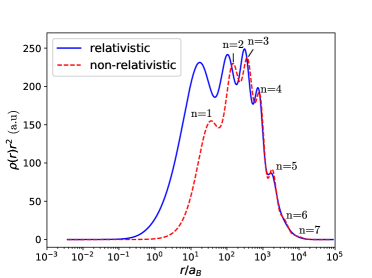
Figure 1: Radial electron density, $4\pi\rho(r)r^{2}$ plot for Og I in both relativistic and non-relativistic approximations. The solid blue line and the dashed red line are non-relativistic and relativistic approximations respectively. The principle quantum peaks have been labeled for the non-relativic plot.

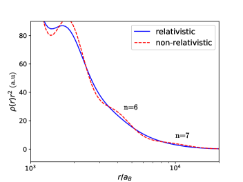
Figure 2: Lower right section of Figure 1.

It has been shown in Ref. Jerabek et al. (2018) using fermion localization that the electron density of Og is smoother than other group 18 analogues which have distinct atomic shells . The cause of this is the large relativistic effects in SHE which effectively smear out the shells into a smoother electron density (the same was shown for the nucleon density). The relativistic effects can also be seen by looking at the radial electron densities with relativistic and non-relativistic approximations. The Hartree-Fock radial electron density for Og is plotted on a logarithmic scale in Figure 1 in both the relativistic and non-relativistic approximations. There are a total of 7 peaks in the radial densities corresponding to the principle quantum numbers $n$ where lower shells have distinct peaks in both the relativistic and non-relativistic approximations. As expected, in the relativistic approximation the inner shells ($n=1,2,3$) shift closer to the nucleus however higher shells are relatively unaffected ($n\geq 4$). This results in a similar density profile for the electrons a large distance away from the nucleus.

In Figure 2 we plot the tail of the density function in Figure 1. Here we see that, while spread out, the principle shell peaks still exist in the non-relativistic approximation. However in the relativistic approximation the density has been smoothed out to such a degree that there are no discernible peaks. This supports the results in ref. Jerabek et al. (2018) where they calculated the electron shell structure of Og I and found that it disappears for external shells due to the high relativistic effects. This can be explained as the large spin-orbit splitting doubles the number of sub-shells which overlap making the overall distribution smooth.

IV Conclusion

In this work we calculated the spectrum and E1 transitions for Og I including the ionisation potential. We demonstrated the accuracy of the calculations by comparing similar calculations of Rn I to experimental data and expect an uncertainty of no more than $|\Delta|\approx 1000$ cm^-1. We found the spectrum of Og I is dense compared to other elements in group 18 with significantly lower ionisation potential and excited states which follows the periodic trend. This compact spectrum introduces an allowed optical E1 transition which does not exist in other group 18 elements which presents a possibility for future experimental measurements. Our work also supports recent findingsJerabek et al. (2018) which suggest the electron shell structure of Og I is less prominent than lighter elements due to large relativistic effects which results in the outer electron density to becoming smooth.

This work was funded in part by the Australian Research Council.

References

- Oganessian et al. (2006) Y. T. Oganessian, V. K. Utyonkov, Y. V. Lobanov, F. S. Abdullin, A. N. Polyakov, R. N. Sagaidak, I. V. Shirokovsky, Y. S. Tsyganov, A. A. Voinov, G. G. Gulbekian, S. L. Bogomolov, B. N. Gikal, A. N. Mezentsev, S. Iliev, V. G. Subbotin, A. M. Sukhov, K. Subotic, V. I. Zagrebaev, G. K. Vostokin, M. G. Itkis, K. J. Moody, J. B. Patin, D. A. Shaughnessy, M. A. Stoyer, N. J. Stoyer, P. A. Wilk, J. M. Kenneally, J. H. Landrum, J. F. Wild, and R. W. Lougheed, Phys. Rev. C 74, 044602 (2006).
- Karol et al. (2016) P. J. Karol, R. C. Barber, B. M. Sherrill, E. Vardaci, and T. Yamazaki, Pure App. Chem 88, 155 (2016).
- Pershina (2009) V. Pershina, Russ. Chem. Rev. 78, 1153 (2009).
- Schwerdtfeger et al. (2015) P. Schwerdtfeger, L. F. Pašteka, A. Punnett, and P. O. Bowman, Nucl. Phys. A 944, 551 (2015).
- Oganessian et al. (2004) Y. T. Oganessian, V. K. Utyonkov, Y. V. Lobanov, F. S. Abdullin, and A. N. Polyakov, Nucl. Phys. A 734, 109 (2004).
- Hamilton et al. (2013) J. H. Hamilton, S. Hofmann, and Y. T. Oganessian, Annu. Rev. Nucl. Part. Sci. 63, 383 (2013).
- Polukhina (2012) N. G. Polukhina, Phys.-Usp. 55, 614 (2012).
- Gopka et al. (2008) V. F. Gopka, A. V. Yushchenko, V. A. Yushchenko, I. V. Panov, and C. Kim, Kinematics Phys. Celestial Bodies 24, 89 (2008).
- Fivet et al. (2007) V. Fivet, P. Quinet, E. Biémont, A. Jorissen, A. V. Yushchenko, and S. Van Eck, Mom. Not. R. Astron. Soc. 380, 781 (2007).
- Dzuba et al. (2017a) V. A. Dzuba, V. V. Flambaum, and J. K. Webb, Phys. Rev. A 95, 062515 (2017a).
- Goriely et al. (2017) S. Goriely, A. Bauswein, and H.-T. Janka, Astrophys. J. Lett. 738, L32 (2017).
- Fuller et al. (2017) G. M. Fuller, A. Kusenko, and V. Takhistov, Phys. Rev. Lett. 119, 061101 (2017).
- Frebel and Beers (2018) A. Frebel and T. C. Beers, Phys. Today 71, 30 (2018).
- Schuetrumpf et al. (2015) B. Schuetrumpf, M. A. Klatt, K. Iida, G. E. Schröder-Turk, J. A. Maruhn, K. Mecke, and P.-G. Reinhard, Phys. Rev. C 91, 025801 (2015).
- Kullie and Saue (2012) O. Kullie and T. Saue, Chem. Phys 395, 54 (2012).
- Shee et al. (2015) A. Shee, S. Knecht, and T. Saue, PPhys. Chem. Chem. Phys. 17 (2015).
- Nash and Bursten (1999) C. S. Nash and B. E. Bursten, Angew. Chem. 38, 115 (1999).
- Nash (2005) C. S. Nash, J. Phys. Chem. A 109, 3493 (2005).
- Schwerdtfeger (2016) P. Schwerdtfeger, EPJ Web Conf. 131, 1 (2016).
- Pitzer (1975) K. S. Pitzer, J. Chem. Phys 63, 1032 (1975).
- Eliav et al. (1996) E. Eliav, U. Kaldor, Y. Ishikawa, and P. Pyykkö, Phys. Rev. Lett. 77, 5350 (1996).
- Pershina et al. (2008) V. Pershina, A. Borschevsky, E. Eliav, and U. Kaldor, J. Chem. Phys 129 (2008).
- Hangele et al. (2012) T. Hangele, M. Dolg, M. Hanrath, X. Cao, and P. Schwerdtfeger, J. Chem. Phys. 136, 214105 (2012).
- Goidenko et al. (2003) I. Goidenko, L. Labzowsky, E. Eliav, U. Kaldor, and P. Pyykkö, Phys. Rev. A 67, 020102 (2003).
- Desclaux (1973) J. P. Desclaux, Atom. Data Nucl. Data Tab 12, 311 (1973).
- Jerabek et al. (2018) P. Jerabek, B. Schuetrumpf, P. Schwerdtfeger, and W. Nazarewicz, Phys. Rev. Lett. 120, 053001 (2018).
- Indelicato et al. (2007) P. Indelicato, J. P. Santos, S. Boucard, and J. P. Desclaux, Euro. Phys. J. D 45, 155 (2007).
- Pyykkö (1988) P. Pyykkö, Chem. Rev. 88, 563 (1988).
- Eliav et al. (2015) E. Eliav, S. Fritzsche, and U. Kaldor, Nucl. Phys. A 944, 518 (2015).
- Thierfelder and Schwerdtfeger (2010) C. Thierfelder and P. Schwerdtfeger, Phys. Rev. A 82, 062503 (2010).
- Kramida et al. (2018) A. Kramida, Yu. Ralchenko, J. Reader, and and NIST ASD Team, NIST Atomic Spectra Database (ver. 5.5.6), [Online]. Available: https://physics.nist.gov/asd [2018, September 25]. National Institute of Standards and Technology, Gaithersburg, MD. (2018).
- Dzuba et al. (2017b) V. A. Dzuba, J. C. Berengut, C. Harabati, and V. V. Flambaum, Phys. Rev. A 95, 012503 (2017b).
- Lackenby et al. (2018) B. G. C. Lackenby, V. A. Dzuba, and V. V. Flambaum, Phys. Rev. A 98, 022518 (2018).
- Dzuba et al. (2018) V. A. Dzuba, V. V. Flambaum, and S. Schiller, Phys. Rev. A 98, 022501 (2018).
- Kelly (1964) H. P. Kelly, Phys. Rev 136, 3B (1964).
- Dzuba (2005) V. A. Dzuba, Phys. Rev. A 71, 032512 (2005).
- Johnson et al. (1988) W. R. Johnson, S. A. Blundell, and J. Sapirstein, Phys. Rev. A 37, 307 (1988).
- Breit (1929) G. Breit, Phys. Rev. 34, 4 (1929).
- Mann and Johnson (1971) J. B. Mann and W. R. Johnson, Phys. Rev. A 4, 1 (1971).
- Dzuba and Flambaum (2016) V. A. Dzuba and V. V. Flambaum, Hyperfine Interactions 237, 160 (2016).
- Flambaum and Ginges (2005) V. V. Flambaum and J. S. M. Ginges, Phys. Rev. A 72, 052115 (2005).
- Morton (2000) D. C. Morton, Astrophys. J. Suppl. Ser. 130, 403 (2000).
- Fuhr and Wiese (1996) J. R. Fuhr and W. L. Wiese, NIST Atomic Transition Probability Tables, 77th ed. (CRC Press, Inc. Boca Raton, FL, 1996).