Constraints on a sub-eV scale sterile neutrino from non-oscillation measurements

Abstract

Anomalies in several short-baseline neutrino oscillation experiments suggest the possible existence of sterile neutrinos at about eV scale having appreciable mixing with the already known three neutrinos. We find that if such a light sterile neutrino exists, through a combined study of the leptonic decays of $\mu^{-}$, $\tau^{-}$, $\pi^{-}$ and $K^{-}$, some semi-leptonic decays of $\tau^{-}$ and the invisible decay width of the $Z$ boson, it is possible to constrain the relevant mixing matrix elements. Furthermore, we compare the constraints, derived by using the method presented here, with the experimental results obtained from short-baseline neutrino oscillation experiments. We find that a single light sterile neutrino cannot satisfy the existing short-baseline neutrino oscillation constraints and explain the anomalies mentioned above. Along the way we provide a number of experimentally clean observables which can be used to directly study the light sterile neutrino independently of the neutrino oscillation experiments.

I Introduction

Sterile neutrinos, first hypothesized by Pontecorvo Pontecorvo:1967fh , are electrically neutral fermions of either Dirac or Majorana nature with no standard weak interaction albeit mixing with the existing active neutrinos. Mathematically, sterile neutrinos are singlets under the gauge symmetry of the standard model (SM) of particle physics. The theoretical studies of sterile neutrinos deal with many diverse new physics scenarios which may include a multitude of sterile neutrinos with masses ranging from below eV scale to close to the Planck mass scale. In this paper we shall focus only on light sterile neutrinos which have masses near the eV scale and we discuss how information from non-oscillation experiments can be used to constrain the mixing matrix elements of active-sterile neutrino mixing.

The existence of one or more light sterile neutrinos near the eV scale can help resolve some of the intriguing ‘anomalies’ observed in short-baseline (SBL) neutrino oscillation experiments, such as the LSND LSND-anomaly , MiniBooNE MiniBooNE-anomaly and Gallium Gallium-anomaly anomalies. In this paper we assume that there exists only one light sterile neutrino $\nu_{\text{s}}$ in addition to the three known active neutrinos ($\nu_{e}$, $\nu_{\mu}$, $\nu_{\tau}$), all of which can be written as linear combination of four neutrino mass eigenstates ($\nu_{1}$, $\nu_{2}$, $\nu_{3}$, $\nu_{4}$):

$$\nu_{\alpha}=\sum_{i=1}^{4}V_{\alpha i}\;\nu_{i}\ ,$$ (1)

where $\alpha=e,\mu,\tau,\text{s}$. We assume that the Pontecorvo-Maki-Nakagawa-Sakata (PMNS) matrix Pontecorvo:1967fh ; Maki:1962mu , the $3\times 3$ matrix that deals with the mixing of $\nu_{e}$, $\nu_{\mu}$, $\nu_{\tau}$ with $\nu_{1}$, $\nu_{2}$, $\nu_{3}$, remains unitary in presence of the sterile neutrino $\nu_{\text{s}}$, while the $4\times 4$ mixing matrix $V$ (which might be unrelated to any see-saw mechanism for generating neutrino mass) can be, in general, non-unitary Cvetic:2017gkt . In this case, the effects of sterile neutrinos will become manifest in the observables associated to charged current interactions of leptons (here repeated labels indicate summation convention, $\ell=e,\mu,\tau$ and $\widehat{\gamma_{\mu}}\equiv\gamma_{\mu}(1-\gamma_{5})$),

$${\cal L}_{W}^{\rm CC} =-\frac{g}{2\sqrt{2}}\,\sum_{\ell=e,\mu,\tau}\,\left[\bar{\ell}\;\widehat{\gamma_{\mu}}\,\nu_{\ell}\right]W^{\mu}+{\rm h.c.}$$

$$=-\frac{g}{2\sqrt{2}}\,\sum_{\ell=e,\mu,\tau}\,\sum_{i=1}^{4}V_{\ell i}\left[\bar{\ell}\;\widehat{\gamma_{\mu}}\,\nu_{i}\right]W^{\mu}+{\rm h.c.},$$ (2)

as well as in neutral current $Z$ boson decays into neutrinos,

$${\cal L}_{Z}^{\rm NC} =-\frac{g}{4\cos\theta_{W}}\,\sum_{\ell=e,\mu,\tau}\,\left[\bar{\nu}_{\ell}\;\widehat{\gamma_{\mu}}\;\nu_{\ell}\right]Z^{\mu}$$

$$=-\frac{g}{4\cos\theta_{W}}\,\sum_{\ell=e,\mu,\tau}\,\sum_{i=1}^{3}\bigg{[}\bar{\nu}_{i}\;\widehat{\gamma_{\mu}}\,\nu_{i}+\left\lvert V_{\ell 4}\right\rvert^{2}\bar{\nu}_{4}\;\widehat{\gamma_{\mu}}\,\nu_{4}$$

$$\qquad+\left(V_{\ell i}^{*}V_{\ell 4}\,\bar{\nu}_{i}\;\widehat{\gamma_{\mu}}\,\nu_{4}+V_{\ell i}V_{\ell 4}^{*}\,\bar{\nu}_{4}\;\widehat{\gamma_{\mu}}\,\nu_{i}\right)\bigg{]}Z^{\mu},$$ (3)

where $g$ is the weak coupling constant and $\theta_{W}$ is the weak mixing angle. The above expression follows from the unitarity of the $3\times 3$ PMNS matrix. It is important to note that to keep our discussion most general we consider the $4\times 4$ mixing matrix to be non-unitary. In some new physics scenarios the sterile neutrino can have a different origin from the active neutrinos, leading to the non-unitarity of the mixing matrix (for a specific model realizing this scenario see for instance Cvetic:2017gkt ). This violation of unitarity, if observed, would imply presence of unknown new physics.

Taking the Lagrangians of Eqs. (2) and (3) into account we shall explore the effects of this hypothetical light sterile neutrino in some precision observables and try to set constraints on its mixing with the known flavor eigenstates. Our purpose is to identify observables that turn out to be the most sensitive ones and present a clean way to determine the mixing matrix elements. Given the lightness of this sterile neutrino, its effects on the different observables considered in this analyses will manifest as an overall normalization factor. Ratios of decay rates turn out to be very useful since they are independent of weak couplings, quark mixings and hadronic form factors. The effects of the sterile neutrino do not cancel in such ratios as long as they do not satisfy lepton universality, which in our case implies $\left\lvert V_{e4}\right\rvert\neq\left\lvert V_{\mu 4}\right\rvert\neq\left\lvert V_{\tau 4}\right\rvert$.

Our paper is organized as follows. In Sec. II we provide a comprehensive analysis of the relevant weak decays, with particular attention to the constraints on active-sterile neutrino mixing matrix elements. We do a combined study of the leptonic decays of $\mu^{-}$, $\tau^{-}$, $\pi^{-}$ and $K^{-}$, some semi-leptonic decays of $\tau^{-}$ as well as the invisible decay of $Z$ boson. We provide all the observables which can be used to constrain the mentioned mixing matrix elements. In Sec. III we perform a numerical study taking all available experimental data and also look for further predictions which can be tested in oscillation and non-oscillation experiments. Finally we conclude in Sec. IV emphasizing the results and the uniqueness of our approach.

II Probing $\left\lvert V_{\ell 4}\right\rvert$ via weak decays

Lepton flavor is an absolutely conserved quantum number in the SM with massless neutrinos. In this limit, we can identify the flavor of neutrinos (or antineutrinos) produced in processes induced by charged weak currents by identifying the flavor of the associated charged lepton, as in the case, for example, of $\mu^{-}\to e^{-}\bar{\nu}_{e}\nu_{\mu}$ decay. However, if neutrinos are massive particles, lepton flavor-violating (LFV) processes like $\mu^{-}\to e^{-}\nu_{\ell}\bar{\nu}_{\ell}$ are possible via a Z-penguin or box diagram at the one loop level. Strictly speaking, the observable process when neutrinos are massive is $\mu^{-}\to e^{-}+$ “missing” because the flavor of neutrinos is not identified. In general, since the light sterile neutrinos, like the active ones, remain undetected at their place of production, any weak decay of the type $X\to Y+a\nu_{\ell}+b\bar{\nu}_{\ell^{\prime}}$ is practically $X\to Y+\text{``missing''}$ where $X$ and $Y$ are some initial and final particle(s) respectively, $\ell,\ell^{\prime}=e,\mu,\tau$ and $a,b=0,1$. We shall assume that the unobserved neutral fermions produced in such weak decays under consideration are either active or sterile neutrinos (or anti-neutrinos). As we shall show, this allows us to set bounds on the mixing matrix elements $\left\lvert V_{\ell 4}\right\rvert$, provided the more sensitive observables to these effects are conveniently chosen.

II.1 Leptonic decays of $\mu^{-}$ and $\tau^{-}$

Let us first consider the leptonic $\mu^{-}$ decay as the reference process. In the presence of a single sterile neutrino, there are four possible contributions to muon decay: $\mu^{-}\to e^{-}\bar{\nu}_{e}\nu_{\mu},\ e^{-}\bar{\nu}_{e}\nu_{4},e^{-}\bar{\nu}_{4}\nu_{\mu}$ and $e^{-}\bar{\nu}_{4}\nu_{4}$, all of which contribute to $\mu^{-}\to e^{-}+\text{``missing"}$. The corresponding rate for the $\mu^{-}\to e^{-}+\text{``missing"}$ is given by,

$$\Gamma_{\mu}=\frac{\left(G_{F}^{0}\right)^{2}}{192\,\pi^{3}}\;\rho_{\mu e}\;\Sigma_{\mu e}\ .$$ (4)

We have defined

$$\rho_{\mu e}=m_{\mu}^{5}\,f\left(m_{e}^{2}/m_{\mu}^{2}\right)\,f_{W}\left(m_{\mu}\right)\,f_{\text{ew}}\left(m_{\mu}\right),$$ (5)

where $m_{\ell}$ denotes the mass of the charged lepton $\ell$, $G_{F}^{0}$ is the Fermi constant if we were to assume no sterile neutrino, $f(x)=1-8x+8x^{3}-x^{4}-12x^{2}\ln x$, $f_{W}(m_{\ell})=1+3/5(m_{\ell}/m_{W})^{2}$ is the finite $W$ mass correction stemming from the $W$ boson propagator, $f_{\text{ew}}\left(m_{\ell}\right)$ are the remaining radiative corrections to the decay rate. Including the effects of the finite mass of electron and the $O\left(\alpha^{2}\right)$ radiative corrections, numerically we have: $f_{\text{ew}}\left(m_{\mu}\right)=0.995802$ Tanabashi:2018oca . The effect of the sterile neutrino is encoded in the factor $\Sigma_{\mu e}$:

$$\Sigma_{\mu e}\equiv\bigg{(}1+\left\lvert V_{e4}\right\rvert^{2}\bigg{)}\left(1+\left\lvert V_{\mu 4}\right\rvert^{2}\right).$$ (6)

The measured value of the effective Fermi constant is given by $G_{F}=G_{F}^{0}\left(\Sigma_{e\mu}\right)^{1/2}=1.1663787(6)\times 10^{-5}\text{ GeV}^{-2}$ Tanabashi:2018oca , obtained from a comparison of the muon decay rate in Eq. (4) and the measured muon lifetime $\tau_{\mu}=1/\Gamma_{\mu}$. As can be realized, it is not possible to quantify the effect of sterile neutrino from $\Gamma_{\mu}$ measurement alone without an independent and precise measurement of $G_{F}^{0}$.

A similar expression holds for the decay rates of $\tau^{-}\to\ell^{-}+{\rm``missing"}$ decays (with $\ell=e,\mu$), which in the presence of an additional sterile neutrino becomes:

$$\Gamma_{\tau}^{\ell}=\frac{\left(G_{F}^{0}\right)^{2}}{192\,\pi^{3}}\;\rho_{\tau\ell}\;\Sigma_{\tau\ell}\ ,$$ (7)

with

$$\rho_{\tau\ell}=m_{\tau}^{5}\,f\left(m_{\ell}^{2}/m_{\tau}^{2}\right)\,f_{W}\left(m_{\tau}\right)\,f_{\text{ew}}^{\ell}\left(m_{\tau}\right),$$ (8)

where we have a similar expression for the $\Sigma_{\tau\ell}$ factor as in Eq. (6), under the corresponding replacement of flavor indices. The numerical values of the radiative corrections are $f_{\text{ew}}^{e}\left(m_{\tau}\right)=0.995722$ and $f_{\text{ew}}^{\mu}\left(m_{\tau}\right)=0.995960$ Tanabashi:2018oca . If we compute the ratio between Eqs. (4) and (7), we obtain

$$\frac{\Gamma_{\tau}^{\ell}}{\Gamma_{\mu}}=\frac{\rho_{\tau\ell}}{\rho_{\mu e}}\;\frac{\Sigma_{\tau\ell}}{\Sigma_{\mu e}}\ .$$ (9)

If we take the ratio of $\Gamma_{\tau}^{e}$ and $\Gamma_{\tau}^{\mu}$ using Eq. (7), we get,

$$\frac{\Gamma_{\tau}^{e}}{\Gamma_{\tau}^{\mu}}=\left(\frac{\rho_{\tau e}}{\rho_{\tau\mu}}\right)\left(\frac{1+\left\lvert V_{e4}\right\rvert^{2}}{1+\left\lvert V_{\mu 4}\right\rvert^{2}}\right).$$ (10)

It is clear from Eqs. (9) and (10) that if there is no lepton universality, i.e. $\left\lvert V_{e4}\right\rvert\neq\left\lvert V_{\mu 4}\right\rvert\neq\left\lvert V_{\tau 4}\right\rvert$, we can find out some observables which can probe the active-sterile mixing, without being worried about the extraction of the Fermi constant $G_{F}^{0}$. Since all the mixing matrix elements $\left\lvert V_{\ell 4}\right\rvert^{2}$ are positive and do not exceed unity, we have $1/2\leq\Sigma_{\tau\ell}/\Sigma_{\mu e},\Sigma_{\tau e}/\Sigma_{\tau\mu}\leq 2$. In practice, given the good agreement of the SM with experimental data for the leptonic decays of $\tau$, we would expect to have $\Sigma_{\tau\ell}/\Sigma_{\mu e}$ very close to $1$.

Note that we can always express the partial decay rates of the decays of $\tau^{-}$ in terms of branching ratios (denoted by $\text{Br}\left(\tau^{-}\to\ell^{-}+\text{``missing''}\right)$) and mean lifetime of $\tau^{-}$ (denoted by $\tau_{\tau}$): $\Gamma_{\tau}^{\ell}=\text{Br}\left(\tau^{-}\to\ell^{-}+\text{``missing''}\right)/\tau_{\tau}$. In this way we obtain the following observables, which are ratios involving the mixing matrix elements $\left\lvert V_{\ell 4}\right\rvert$,

$$R_{\tau/e} \equiv\frac{1+\left\lvert V_{\tau 4}\right\rvert^{2}}{1+\left\lvert V_{e4}\right\rvert^{2}}=\frac{\text{Br}\left(\tau\to\mu+\text{``missing''}\right)}{\text{Br}\left(\mu\to e+\text{``missing''}\right)}\frac{\tau_{\mu}}{\tau_{\tau}}\frac{\rho_{\mu e}}{\rho_{\tau\mu}}\ ,$$ (11a)

$$R_{\tau/\mu} \equiv\frac{1+\left\lvert V_{\tau 4}\right\rvert^{2}}{1+\left\lvert V_{\mu 4}\right\rvert^{2}}=\frac{\text{Br}\left(\tau\to e+\text{``missing''}\right)}{\text{Br}\left(\mu\to e+\text{``missing''}\right)}\frac{\tau_{\mu}}{\tau_{\tau}}\frac{\rho_{\mu e}}{\rho_{\tau e}}\ ,$$ (11b)

$$R_{e/\mu} \equiv\frac{1+\left\lvert V_{e4}\right\rvert^{2}}{1+\left\lvert V_{\mu 4}\right\rvert^{2}}=\frac{\text{Br}\left(\tau\to e+\text{``missing''}\right)}{\text{Br}\left(\tau\to\mu+\text{``missing''}\right)}\frac{\rho_{\tau\mu}}{\rho_{\tau e}}\ .$$ (11c)

These three observables are not independent, by definition, since $R_{\tau/e}\,R_{e/\mu}=R_{\tau/\mu}$. Therefore, only two out of these three ratios would be useful for our numerical analysis and we would need some extra independent observable(s) in order to constrain the three active-sterile mixing matrix elements.

It is important to note that the ratio observables $R_{\tau/e}$, $R_{e/\mu}$ and $R_{\tau/\mu}$ actually probe the unitarity of the $4\times 4$ mixing matrix. If we were to relax the assumption that the $3\times 3$ PMNS matrix is unitary, the ratio observables take the form

$$R_{\ell/\ell^{\prime}}=\left(\sum_{i=1}^{4}\left\lvert V_{\ell i}\right\rvert^{2}\right)/\left(\sum_{j=1}^{4}\left\lvert V_{\ell^{\prime}j}\right\rvert^{2}\right),$$ (12)

where $\ell\neq\ell^{\prime}$ and $\ell,\ell^{\prime}=e,\mu,\tau$. It is clear from Eq. (12) that $R_{\ell/\ell^{\prime}}=1$ only when both $\sum_{i=1}^{4}\left\lvert V_{\ell i}\right\rvert^{2}=1$ and $\sum_{j=1}^{4}\left\lvert V_{\ell^{\prime}j}\right\rvert^{2}~{}=~{}1$. It should be noted that if one were to consider an $n\times n$ active-sterile mixing matrix with $n>4$ in some new physics model, then the summations in Eq. (12) would run from $1$ to $n$. Thus, $R_{\ell/\ell^{\prime}}$ can also probe the unitarity of such an active-sterile mixing matrix in the most general scenario.

II.2 Semileptonic decays of $\tau^{-}$ and leptonic decays of $\pi^{-}$ and $K^{-}$

Ratios of semileptonic decays of $\tau^{-}$ and leptonic decays of $\pi^{-}$ and $K^{-}$ can also be useful to constrain the mixings of a light sterile neutrino. Let us consider the $\tau^{-}\to P^{-}\nu_{\tau}$ and $P^{-}\to\ell^{-}\bar{\nu}_{\ell}$ decays ($P=\pi$ or $K$ mesons and $\ell=e$ or $\mu$), which are the most precisely measured processes of this type. In the presence of a light sterile neutrino, the decay rates of these processes are given by:

$$\Gamma_{\tau\to P\nu}=\frac{\left(G_{F}^{0}\right)^{2}\left\lvert V_{uq}\right\rvert^{2}}{16\pi}f_{P}^{2}\,m_{\tau}^{3}\left(1-\frac{m_{P}^{2}}{m_{\tau}^{2}}\right)^{2}\delta_{\tau}^{P}\left(1+\left\lvert V_{\tau 4}\right\rvert^{2}\right)\ ,$$ (13)

and

$$\Gamma_{P\to\ell\nu}=\frac{\left(G_{F}^{0}\right)^{2}\left\lvert V_{uq}\right\rvert^{2}}{8\pi}f_{P}^{2}\,m_{\ell}^{2}\,m_{P}\left(1-\frac{m_{\ell}^{2}}{m_{P}^{2}}\right)^{2}\delta_{P}^{\ell}\left(1+\left\lvert V_{\ell 4}\right\rvert^{2}\right)\ .$$ (14)

In the above expressions, $f_{P}$ denotes the decay constant of the $P^{-}$ meson, which can be calculated from Lattice QCD, $V_{uq}$ (with $q=d(s)$ for $P=\pi(K)$ mesons) is the Cabibbo-Kobayashi-Maskawa (CKM) matrix element and $\delta_{\tau}^{P}$ (or $\delta_{P}^{\ell}$) denotes the radiative corrections to $\tau\to P\nu$ (or $P\to\ell\nu$) decay.

The ratio of the these decays,

$$\frac{\Gamma_{\tau\to P\nu}}{\Gamma_{P\to\ell\nu}}=\frac{m_{P}^{3}}{2m_{\ell}^{2}m_{\tau}}\left(\frac{m_{\tau}^{2}-m_{P}^{2}}{m_{P}^{2}-m_{\ell}^{2}}\right)^{2}\left(\frac{\delta_{\tau}^{P}}{\delta_{P}^{\ell}}\right)\left(\frac{1+\left\lvert V_{\tau 4}\right\rvert^{2}}{1+\left\lvert V_{\ell 4}\right\rvert^{2}}\right)\ ,$$ (15)

is independent of the parameters related to the hadronic vertex and can provide a clean information about the active-sterile mixing matrix elements provided there is no lepton universality. Furthermore, the ratio of electron and muon channels in $P$ meson decays,

$$\frac{\Gamma_{P\to e\nu}}{\Gamma_{P\to\mu\nu}}=\frac{m_{e}^{2}}{m_{\mu}^{2}}\left(\frac{m_{P}^{2}-m_{e}^{2}}{m_{P}^{2}-m_{\mu}^{2}}\right)^{2}\left(\frac{\delta_{P}^{e}}{\delta_{P}^{\mu}}\right)\left(\frac{1+\left\lvert V_{e4}\right\rvert^{2}}{1+\left\lvert V_{\mu 4}\right\rvert^{2}}\right)\ ,$$ (16)

can also be used to study the active-sterile mixing matrix elements since it is independent of hadronic inputs and common terms of radiative corrections also cancel in the ratio.

The radiative corrections can be split into a short-distance (SD) and a long-distance (LD) parts: $\delta=\delta(SD)+\delta(LD)$. The dominant contribution to SD corrections in $\tau$ and $P$ meson decays is given by

$$\delta_{X}^{Y}(SD)=1+\frac{2\alpha}{\pi}\ln\left(\frac{m_{Z}}{m_{X}}\right)\ .$$ (17)

The computation of the LD parts are more difficult to evaluate, since they depend on the details of the strong interactions in the transition regime (1-2 GeV), which involve usage of phenomenological models including contributions from possible resonances as well as scalar QED, so that one can consider the meson-photon interactions beyond the point-meson approximation LD:difficulty ; Decker:1994ea ; Cirigliano:2007ga . For numerical analysis we shall use the ratio of radiative corrections in the semileptonic $\tau$ decays as given in Ref. Decker:1994ea :

$$\frac{\delta_{\tau}^{P}}{\delta_{P}^{\mu}}=\begin{cases}1.0016\pm 0.0014,&\text{ for }P=\pi^{-}\\ 1.0090\pm 0.0022,&\text{ for }P=K^{-}\end{cases}\ .$$ (18)

Similarly, the ratio of $O(\alpha)$ radiative corrections for $P$ meson decays is given by Cirigliano:2007ga :

$$\frac{\delta_{P}^{e}}{\delta_{P}^{\mu}}=\begin{cases}0.9625\pm 0.0001,&\text{ for }P=\pi^{-}\\ 0.9642\pm 0.0004,&\text{ for }P=K^{-}\end{cases}\ .$$ (19)

Once again, replacing the partial decay rates in terms of branching ratios and lifetimes we can define, by using Eqs. (15) and (16), the equivalent ratio observables as in Eq. (11):

$$R_{\tau/e} =\frac{\text{Br}\left(\tau\to P\nu\right)}{\text{Br}\left(P\to e\nu\right)}\frac{\tau_{P}}{\tau_{\tau}}\frac{2m_{e}^{2}m_{\tau}}{m_{P}^{3}}\left(\frac{m_{P}^{2}-m_{e}^{2}}{m_{\tau}^{2}-m_{P}^{2}}\right)^{2}\left(\frac{\delta_{P}^{e}}{\delta_{\tau}^{P}}\right)\ ,$$ (20a)

$$R_{\tau/\mu} =\frac{\text{Br}\left(\tau\to P\nu\right)}{\text{Br}\left(P\to\mu\nu\right)}\frac{\tau_{P}}{\tau_{\tau}}\frac{2m_{\mu}^{2}m_{\tau}}{m_{P}^{3}}\left(\frac{m_{P}^{2}-m_{\mu}^{2}}{m_{\tau}^{2}-m_{P}^{2}}\right)^{2}\left(\frac{\delta_{P}^{\mu}}{\delta_{\tau}^{P}}\right)\ ,$$ (20b)

$$R_{e/\mu} =\frac{\text{Br}\left(P\to e\nu\right)}{\text{Br}\left(P\to\mu\nu\right)}\frac{m_{\mu}^{2}}{m_{e}^{2}}\left(\frac{m_{P}^{2}-m_{\mu}^{2}}{m_{P}^{2}-m_{e}^{2}}\right)^{2}\left(\frac{\delta_{P}^{\mu}}{\delta_{P}^{e}}\right)\ .$$ (20c)

It must be noted that each ratio defined above has got two values, one corresponding to $P=\pi$ and the other for $P=K$. Even though we did not get any extra observables here, we can probe the same observables from a different set of decays than the purely leptonic decays of $\mu$ and $\tau$ as given in Eq. (11). In fact, if we consider only those decays that are mediated by charged current interaction, we shall be constrained to consider decays of the type $X\to Y+a\nu_{\ell}+b\bar{\nu}_{\ell^{\prime}}$, with $\ell,\ell^{\prime}=e,\mu,\tau$ and $\ell\neq\ell^{\prime}$, $a,b=0,1$ and $X$, $Y$ being appropriate particles. From such decays we can extract only the ratios $R_{\tau/e}$, $R_{\tau/\mu}$ and $R_{e/\mu}$ and nothing more unless we use some other independent information such as $G_{F}^{0}$ or hadronic form factors or CKM matrix elements. For this reason, considering the weak neutral current processes can be useful.

II.3 Invisible width of the $Z$ boson and the number of light active neutrinos

In the presence of a light sterile neutrino, the contributions to the ‘invisible’ decay width of the $Z$ gauge boson that stem from Eq. (3) are: $\bar{\nu}_{\ell}\nu_{\ell},\bar{\nu}_{\ell}\nu_{4},\bar{\nu}_{4}\nu_{\ell}$ and $\bar{\nu}_{4}\nu_{4}$. The invisible width of $Z$ is, therefore, given by:

$$\Gamma_{\text{inv}}=\frac{G_{F}^{0}m_{Z}^{3}}{12\sqrt{2}\,\pi}\sum_{\ell=e,\mu,\tau}\left(1+\left\lvert V_{\ell 4}\right\rvert^{2}\right)^{2},$$ (21)

where $m_{Z}$ denotes the mass of the $Z$ boson. It is interesting to note that the Fermi constant used in Eq. (21) is extracted from the muon decay, which under our assumption of one sterile neutrino leads to Eq. (4). Therefore, in terms of the measured Fermi constant $G_{F}$, the invisible width of $Z$ is given by,

$$\Gamma_{\text{inv}}=\frac{G_{F}\,m_{Z}^{3}}{12\sqrt{2}\,\pi}\frac{1}{\sqrt{\Sigma_{\mu e}}}\sum_{\ell=e,\mu,\tau}\left(1+\left\lvert V_{\ell 4}\right\rvert^{2}\right)^{2}.$$ (22)

If we consider $V_{\ell 4}=0$, we get the expression for $\Gamma_{\text{inv}}^{\text{SM}}$ which is the invisible width of the $Z$ boson in the SM. It is well known that the number of light neutrinos ($N_{\nu}$) is extracted from observed invisible width of $Z$ boson by using the expression,

$$\frac{N_{\nu}}{3}=\frac{\Gamma_{\text{inv}}}{\Gamma_{\text{inv}}^{\text{SM}}}.$$ (23)

Thus, we can express $N_{\nu}$ in terms of the active-sterile mixing matrix elements as follows,

$$N_{\nu}=\frac{1}{\sqrt{\Sigma_{\mu e}}}\sum_{\ell=e,\mu,\tau}\left(1+\left\lvert V_{\ell 4}\right\rvert^{2}\right)^{2}.$$ (24)

It is clear that $N_{\nu}$ can now be used in conjunction with the ratio operators $R_{\tau/e}$, $R_{\tau/\mu}$ and $R_{e/\mu}$ to constrain the active-sterile mixing matrix elements. From Refs. Tanabashi:2018oca ; ALEPH:2005ab we get the number of light neutrinos to be $N_{\nu}=2.9840\pm 0.0082$.

II.4 Energy spectrum of charged lepton in leptonic tau decay

Till now we have considered fully phase-space integrated partial decay rates for some well chosen decays as a means to constrain the active-sterile mixing. It is interesting to ask whether differential partial decay rates or distributions can be used to look for signatures of the sterile neutrino. In presence of one light sterile neutrino, the energy distribution of the final charged lepton $\ell$ in the decay $\tau\to\ell+\text{``missing''}$ gets modified as follows,

$$\frac{d\Gamma\left(\tau\to\ell+\text{``missing''}\right)}{dE_{\ell}} =\left(\frac{32m_{\tau}}{\rho^{\prime}_{\mu e}\,\tau_{\mu}}\right)\left(3E_{\ell}E_{\ell}^{\rm max}-m_{\ell}^{2}-2E_{\ell}^{2}\right)$$

$$\qquad\times\sqrt{E_{\ell}^{2}-m_{\ell}^{2}}\left(\frac{\Sigma_{\tau\ell}}{\Sigma_{\mu e}}\right)\ ,$$ (25)

where $\rho^{\prime}_{\mu e}=m_{\mu}^{5}\,f\left(m_{e}^{2}/m_{\mu}^{2}\right)$ and $E_{\ell}^{\rm max}=(m_{\tau}^{2}+m_{\ell}^{2})/2m_{\tau}$ with $\ell=e,\mu$. This expression does not contain the effects of radiative corrections to the lepton spectrum. It is important to note that this is not a normalized distribution since in that case the effect of sterile neutrinos will cancel during normalization. In Fig. 1 we plot the energy distribution of the muon in $\tau^{-}\to\mu^{-}+{\rm missing}$ decays. We have chosen $0.9\leq\Sigma_{\tau\mu}/\Sigma_{\mu e}\leq 1.1$ as an example for the range of the free parameter. The effect of the sterile neutrino is the same over the whole spectrum although it is more discernible at the end-point of the energy spectrum.

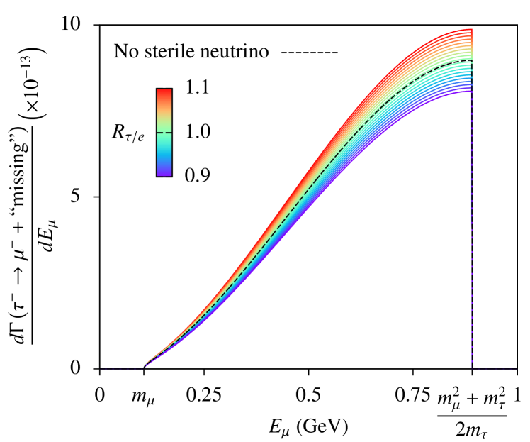
Figure 1: Muon energy spectrum in $\tau^{-}\to\mu^{-}+\text{``missing''}$ decays for values of $R_{\tau/e}=\Sigma_{\tau\mu}/\Sigma_{\mu e}$ in the range $(0.9,1.1)$ using Eq. (25). We have considered lepton non-universality here, i.e. $\left\lvert V_{e4}\right\rvert\neq\left\lvert V_{\mu 4}\right\rvert\neq\left\lvert V_{\tau 4}\right\rvert$, as otherwise $R_{\tau/e}=1$ even for the case of one sterile neutrino.

It is important to note that in order to get a prediction for the effect of sterile neutrino on the energy spectrum as per the present data, we must first constrain the individual mixing matrix elements using our set of observables.

II.5 Analytical solutions for $\left\lvert V_{\ell 4}\right\rvert^{2}$ in terms of observables

We have four observables ($R_{\tau/e}$, $R_{\tau/\mu}$, $R_{e/\mu}$ and $N_{\nu}$) which can be defined in terms of three active-sterile mixing matrix elements ($\left\lvert V_{e4}\right\rvert^{2}$, $\left\lvert V_{\mu 4}\right\rvert^{2}$ and $\left\lvert V_{\tau 4}\right\rvert^{2}$) as shown in Eqs. (11) and (24). Since the three ratio observables of Eq. (11) are not independent, we can always consider $N_{\nu}$ and any two out of the three ratios to solve for the mixing matrix elements. This gives rise to three closely related schemes of analytical solutions. In Sec. III we shall present our numerical analysis following all the three schemes.

Scheme A: In this scheme we shall use $R_{\tau/\mu}$, $R_{e/\mu}$ and $N_{\nu}$ to solve for the mixing matrix elements. From Eqs. (6), (11b) and (11c) it is straightforward to get,

$$\Sigma_{\mu e} =R_{e/\mu}\left(1+\left\lvert V_{\mu 4}\right\rvert^{2}\right)^{2},$$ (26a)

$$\left\lvert V_{\tau 4}\right\rvert^{2} =R_{\tau/\mu}\left(1+\left\lvert V_{\mu 4}\right\rvert^{2}\right)-1,$$ (26b)

$$\left\lvert V_{e4}\right\rvert^{2} =R_{e/\mu}\left(1+\left\lvert V_{\mu 4}\right\rvert^{2}\right)-1.$$ (26c)

Substituting Eq. (26) in Eq. (24) and simplifying we get

$$\left\lvert V_{\mu 4}\right\rvert^{2}=\frac{N_{\nu}\sqrt{R_{e/\mu}}}{1+R_{e/\mu}^{2}+R_{\tau/\mu}^{2}}-1.$$ (27)

Finally substituting Eq. (27) in Eqs. (26b) and (26c) we get,

$$\left\lvert V_{\tau 4}\right\rvert^{2}=\frac{N_{\nu}\,R_{\tau/\mu}\sqrt{R_{e/\mu}}}{1+R_{e/\mu}^{2}+R_{\tau/\mu}^{2}}-1,$$ (28a)

$$\left\lvert V_{e4}\right\rvert^{2}=\frac{N_{\nu}\,R_{e/\mu}^{3/2}}{1+R_{e/\mu}^{2}+R_{\tau/\mu}^{2}}-1.$$ (28b)

Thus Eqs. (27) and (28) express the active-sterile mixing matrix elements in terms of observables $R_{\tau/\mu}$, $R_{e/\mu}$ and $N_{\nu}$.

Scheme B: In this scheme we shall use the observables $R_{\tau/e}$, $R_{e/\mu}$ and $N_{\nu}$. The expressions for active-sterile mixing matrix elements in this scheme are obtained from Eqs. (27) and (28) by making use of the identity $R_{\tau/\mu}=R_{\tau/e}\,R_{e/\mu}$. Thus, in this scheme we have,

$$\left\lvert V_{e4}\right\rvert^{2}=\frac{N_{\nu}\,R_{e/\mu}^{3/2}}{1+R_{e/\mu}^{2}\left(1+R_{\tau/e}^{2}\right)}-1,$$ (29a)

$$\left\lvert V_{\mu 4}\right\rvert^{2}=\frac{N_{\nu}\sqrt{R_{e/\mu}}}{1+R_{e/\mu}^{2}\left(1+R_{\tau/e}^{2}\right)}-1,$$ (29b)

$$\left\lvert V_{\tau 4}\right\rvert^{2}=\frac{N_{\nu}\,R_{\tau/e}\,R_{e/\mu}^{3/2}}{1+R_{e/\mu}^{2}\left(1+R_{\tau/e}^{2}\right)}-1.$$ (29c)

Scheme C: In this scheme we shall use the observables $R_{\tau/e}$, $R_{\tau/\mu}$ and $N_{\nu}$. The expressions for active-sterile mixing matrix elements in this scheme are obtained from Eqs. (27) and (28) by making use of the identity $R_{e/\mu}=R_{\tau/\mu}/R_{\tau/e}$. Thus, in this scheme we have,

$$\left\lvert V_{e4}\right\rvert^{2}=\frac{N_{\nu}\,R_{\tau/\mu}^{3/2}\sqrt{R_{\tau/e}}}{R_{\tau/e}^{2}+R_{\tau/\mu}^{2}+R_{\tau/e}^{2}\,R_{\tau/\mu}^{2}}-1,$$ (30a)

$$\left\lvert V_{\mu 4}\right\rvert^{2}=\frac{N_{\nu}\,R_{\tau/e}^{3/2}\sqrt{R_{\tau/\mu}}}{R_{\tau/e}^{2}+R_{\tau/\mu}^{2}+R_{\tau/e}^{2}\,R_{\tau/\mu}^{2}}-1,$$ (30b)

$$\left\lvert V_{\tau 4}\right\rvert^{2}=\frac{N_{\nu}\,R_{\tau/e}^{3/2}R_{\tau/\mu}^{3/2}}{R_{\tau/e}^{2}+R_{\tau/\mu}^{2}+R_{\tau/e}^{2}\,R_{\tau/\mu}^{2}}-1.$$ (30c)

It is important to note that the ratio observables can be determined by using either Eq. (11) or (20). In the numerical analysis ahead in Sec. III we shall consider both these options. Once we know the values of $\left\lvert V_{\ell 4}\right\rvert^{2}$ it would be interesting to know what would be their impact on short-baseline neutrino oscillation experiments.

II.6 Impact of $\left\lvert V_{\ell 4}\right\rvert$ on short-baseline neutrino oscillation

In short-baseline (SBL) neutrino oscillation experiments, where the active-sterile neutrino oscillations are easier to observe, the effective probability of neutrino oscillations from an initial flavor state $\nu_{\alpha}$ to a final flavor state $\nu_{\beta}$ is given by

$$P_{\alpha\beta}^{\text{(SBL)}}\simeq\left\lvert\delta_{\alpha\beta}-\sin^{2}2\theta_{\alpha\beta}\,\sin^{2}\left(\frac{\Delta m_{\text{SBL}}^{2}\,L}{4E}\right)\right\rvert,$$ (31)

where $L$ is the distance between the neutrino source and the detector, $E$ is the energy of the neutrino beam, $\Delta m_{\text{SBL}}^{2}$ is the new squared-mass difference corresponding to oscillations between the sterile and active neutrinos, and the oscillation amplitude is given by,

$$\sin^{2}2\theta_{\alpha\beta}=4\left\lvert V_{\alpha 4}\right\rvert^{2}\left\lvert\delta_{\alpha\beta}-\left\lvert V_{\beta 4}\right\rvert^{2}\right\rvert.$$ (32)

We are interested in $\sin^{2}2\theta_{\mu e}$, $\sin^{2}2\theta_{ee}$ and $\sin^{2}2\theta_{\mu\mu}$ which can be easily constrained once we know $\left\lvert V_{e4}\right\rvert^{2}$ and $\left\lvert V_{\mu 4}\right\rvert^{2}$ by using our schemes A, B, C as discussed before.

III Numerical analysis and discussion

In order to numerically estimate the active-sterile mixing matrix elements using the expressions obtained in the previous section under schemes A, B and C, we have used all the precise experimental results for branching ratios, lifetimes, masses, radiative corrections and the number of light neutrinos $N_{\nu}$ as reported by the Particle Data Book Tanabashi:2018oca . In the numerical study we have used Eq. (11), (20b) and (20c) for the ratio observables considering both $P=\pi$ and $P=K$. We have done a simple propagation of errors following the method of quadrature. Our numerical calculation gives the following values for the ratio observables,

$$R_{\tau/e} =\ \ 1.00667\pm 0.00293\quad\text{(Using Eq.~{}\eqref{eq:R-t-e})},$$ (33a)

$$R_{\tau/\mu} =\begin{cases}1.00290\pm 0.00287&\text{(Using Eq.~{}\eqref{eq:R-t-m})}\\ 0.99406\pm 0.00594&\text{(Using Eq.~{}\eqref{eq:Rtm} for $P=\pi$)}\\ 0.97807\pm 0.01443&\text{(Using Eq.~{}\eqref{eq:Rtm} for $P=K$)}\end{cases},$$ (33b)

$$R_{e/\mu} =\begin{cases}0.99626\pm 0.00320&\text{(Using Eq.~{}\eqref{eq:R-e-m})}\\ 0.99589\pm 0.00324&\text{(Using Eq.~{}\eqref{eq:Rem} for $P=\pi$)}\\ 1.00436\pm 0.00479&\text{(Using Eq.~{}\eqref{eq:Rem} for $P=K$)}\end{cases}.$$ (33c)

It is quite clear from these results that all the estimates for the ratio observables are consistent with $1$ within $2\sigma$ standard deviations. This implies that the $4\times 4$ mixing matrix is unitary irrespective of whether we consider the $3\times 3$ PMNS matrix to be unitary or not. Using the value of $R_{\tau/e}$ from Eq. (33a) in Eq. (25) we can plot the unnormalized energy distribution of the muon in the decay $\tau^{-}\to\mu^{-}+\text{``missing''}$, as shown in Fig. 2. It is clear from this distribution that the current data from weak decays is consistent with absence of light sterile neutrinos. Since the search for light sterile neutrinos is traditionally done via short-baseline neutrino oscillation experiments, looking at the estimates of active-sterile mixing matrix elements as well as the oscillation amplitude would be very useful.

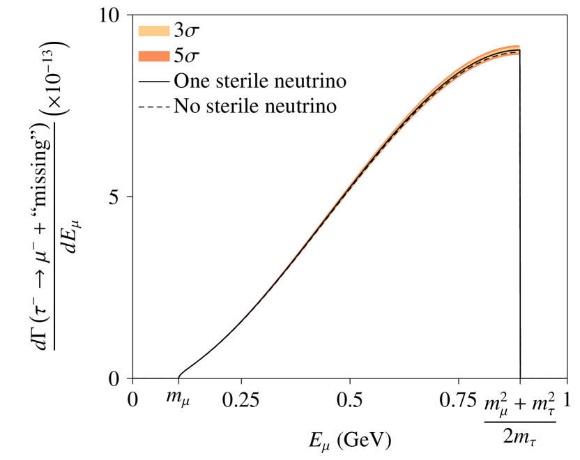
Figure 2: The unnormalized muon energy distribution in the decay $\tau^{-}\to\mu^{-}+\text{``missing''}$ considering $\Sigma_{\tau\mu}/\Sigma_{\mu e}=R_{\tau/e}$ from Eq. (33a).

Predicted values for $\left\lvert V_{e4}\right\rvert^{2}$ Scheme A Scheme C $R_{e/\mu}$ $R_{\tau/e}$ Eq. (11c) Eq. (20c) Eq. (11a) $P=\pi$ $P=K$ $R_{\tau/\mu}$ Eq. (11b) $0.01036\pm 0.00425$ $0.01067\pm 0.00428$ $0.00365\pm 0.00517$ $0.01036\pm 0.00276$ Eq. (20b) $P=\pi$ $0.00450\pm 0.00549$ $0.00481\pm 0.00551$ $0.00222\pm 0.00623$ $0.01186\pm 0.00290$ $P=K$ $0.00614\pm 0.01037$ $0.00583\pm 0.01038$ $0.01288\pm 0.01079$ $0.01478\pm 0.00386$ Scheme B $R_{\tau/e}$ $0.01036\pm 0.00277$ $0.01043\pm 0.00277$ $0.00905\pm 0.00283$

(a)

Predicted values for $\left\lvert V_{\mu 4}\right\rvert^{2}$ Scheme A Scheme C $R_{e/\mu}$ $R_{\tau/e}$ Eq. (11c) Eq. (20c) Eq. (11a) $P=\pi$ $P=K$ $R_{\tau/\mu}$ Eq. (11b) $0.00665\pm 0.00337$ $0.00659\pm 0.00337$ $0.00798\pm 0.00342$ $0.00665\pm 0.00361$ Eq. (20b) $P=\pi$ $0.00076\pm 0.00485$ $0.00070\pm 0.00485$ $0.00214\pm 0.00486$ $0.00067\pm 0.00565$ $P=K$ $0.00992\pm 0.01007$ $0.00998\pm 0.01008$ $0.00848\pm 0.01003$ $0.01403\pm 0.01244$ Scheme B $R_{\tau/e}$ $0.00665\pm 0.00381$ $0.00634\pm 0.00383$ $0.01336\pm 0.00480$

(b)

Predicted values for $\left\lvert V_{\tau 4}\right\rvert^{2}$ Scheme A Scheme C $R_{e/\mu}$ $R_{\tau/e}$ Eq. (11c) Eq. (20c) Eq. (11a) $P=\pi$ $P=K$ $R_{\tau/\mu}$ Eq. (11b) $0.00376\pm 0.00294$ $0.00370\pm 0.00294$ $0.00510\pm 0.00300$ $0.00376\pm 0.00278$ Eq. (20b) $P=\pi$ $0.00670\pm 0.00342$ $0.00664\pm 0.00342$ $0.00806\pm 0.00349$ $0.00527\pm 0.00292$ $P=K$ $0.01222\pm 0.00582$ $0.01216\pm 0.00582$ $0.01364\pm 0.00589$ $0.00821\pm 0.00389$ Scheme B $R_{\tau/e}$ $0.00376\pm 0.00279$ $0.00382\pm 0.00279$ $0.00244\pm 0.00284$

(c)

Table 1: Predicted values for $\left\lvert V_{\ell 4}\right\rvert^{2}$ (with $\ell=e,\mu,\tau$) from weak decays following schemes A, B and C. The pairs of ratio observables used in these predictions are $R_{\tau/\mu}$ and $R_{e/\mu}$ for scheme A, $R_{e/\mu}$ and $R_{\tau/e}$ for scheme B and, finally, $R_{\tau/\mu}$ and $R_{\tau/e}$ for scheme C. In all the schemes the observable $N_{\nu}$, the number of light neutrinos, is used.

Predicted values for $\sin^{2}2\theta_{\mu e}=4\left\lvert V_{\mu 4}\right\rvert^{2}\left\lvert V_{e4}\right\rvert^{2}$ Scheme A Scheme C $R_{e/\mu}$ $R_{\tau/e}$ Eq. (11c) Eq. (20c) Eq. (11a) $P=\pi$ $P=K$ $R_{\tau/\mu}$ Eq. (11b) $\left(2.76\pm 1.80\right)\times 10^{-4}$ $\left(2.81\pm 1.83\right)\times 10^{-4}$ $\left(1.17\pm 1.72\right)\times 10^{-4}$ $\left(2.76\pm 1.67\right)\times 10^{-4}$ Eq. (20b) $P=\pi$ $\left(0.14\pm 0.89\right)\times 10^{-4}$ $\left(0.14\pm 0.95\right)\times 10^{-4}$ $\left(0.19\pm 0.68\right)\times 10^{-4}$ $\left(0.32\pm 2.68\right)\times 10^{-4}$ $P=K$ $\left(2.44\pm 4.80\right)\times 10^{-4}$ $\left(2.33\pm 4.77\right)\times 10^{-4}$ $\left(4.36\pm 6.33\right)\times 10^{-4}$ $\left(8.29\pm 7.67\right)\times 10^{-4}$ Scheme B $R_{\tau/e}$ $\left(2.76\pm 1.74\right)\times 10^{-4}$ $\left(2.64\pm 1.75\right)\times 10^{-4}$ $\left(4.84\pm 2.30\right)\times 10^{-4}$

(a)

Predicted values for $\sin^{2}2\theta_{ee}=4\left\lvert V_{e4}\right\rvert^{2}\left\lvert 1-\left\lvert V_{e4}\right\rvert^{2}\right\rvert$ Scheme A Scheme C $R_{e/\mu}$ $R_{\tau/e}$ Eq. (11c) Eq. (20c) Eq. (11a) $P=\pi$ $P=K$ $R_{\tau/\mu}$ Eq. (11b) $\left(4.10\pm 1.67\right)\times 10^{-2}$ $\left(4.22\pm 1.67\right)\times 10^{-2}$ $\left(1.46\pm 2.05\right)\times 10^{-2}$ $\left(4.10\pm 1.08\right)\times 10^{-2}$ Eq. (20b) $P=\pi$ $\left(1.79\pm 2.18\right)\times 10^{-2}$ $\left(1.92\pm 2.18\right)\times 10^{-2}$ $\left(0.88\pm 2.48\right)\times 10^{-2}$ $\left(4.69\pm 1.14\right)\times 10^{-2}$ $P=K$ $\left(2.44\pm 4.10\right)\times 10^{-2}$ $\left(2.32\pm 4.10\right)\times 10^{-2}$ $\left(5.08\pm 4.20\right)\times 10^{-2}$ $\left(5.82\pm 1.50\right)\times 10^{-2}$ Scheme B $R_{\tau/e}$ $\left(4.10\pm 1.09\right)\times 10^{-2}$ $\left(4.13\pm 1.09\right)\times 10^{-2}$ $\left(3.59\pm 1.11\right)\times 10^{-2}$

(b)

Predicted values for $\sin^{2}2\theta_{\mu\mu}=4\left\lvert V_{\mu 4}\right\rvert^{2}\left\lvert 1-\left\lvert V_{\mu 4}\right\rvert^{2}\right\rvert$ Scheme A Scheme C $R_{e/\mu}$ $R_{\tau/e}$ Eq. (11c) Eq. (20c) Eq. (11a) $P=\pi$ $P=K$ $R_{\tau/\mu}$ Eq. (11b) $\left(2.64\pm 1.33\right)\times 10^{-2}$ $\left(2.62\pm 1.33\right)\times 10^{-2}$ $\left(3.17\pm 1.35\right)\times 10^{-2}$ $\left(2.64\pm 1.43\right)\times 10^{-2}$ Eq. (20b) $P=\pi$ $\left(0.31\pm 1.94\right)\times 10^{-2}$ $\left(0.28\pm 1.94\right)\times 10^{-2}$ $\left(0.85\pm 1.94\right)\times 10^{-2}$ $\left(0.27\pm 2.26\right)\times 10^{-2}$ $P=K$ $\left(3.93\pm 3.95\right)\times 10^{-2}$ $\left(3.95\pm 3.95\right)\times 10^{-2}$ $\left(3.36\pm 3.94\right)\times 10^{-2}$ $\left(5.53\pm 4.84\right)\times 10^{-2}$ Scheme B $R_{\tau/e}$ $\left(2.64\pm 1.50\right)\times 10^{-2}$ $\left(2.52\pm 1.51\right)\times 10^{-2}$ $\left(5.27\pm 1.87\right)\times 10^{-2}$

(c)

Table 2: Values for $\sin^{2}2\theta_{\mu e}$, $\sin^{2}2\theta_{ee}$ and $\sin^{2}2\theta_{\mu\mu}$ predicted by using the values of $\left\lvert V_{e4}\right\rvert^{2}$ and $\left\lvert V_{\mu 4}\right\rvert^{2}$ (see Tables 1a and 1b respectively) predicted from weak decays following schemes A, B and C.

Using the values of ratio observables as shown in Eq. (33) we can predict the values for $\left\lvert V_{\ell 4}\right\rvert^{2}$ (with $\ell=e,\mu,\tau$) following schemes A, B and C. The predictions for $\left\lvert V_{e4}\right\rvert^{2}$, $\left\lvert V_{\mu 4}\right\rvert^{2}$ and $\left\lvert V_{\tau 4}\right\rvert^{2}$ are tabulated in Tables 1a, 1b and 1c respectively. Taking the average of these determined values we get,

$$\overline{\left\lvert V_{e4}\right\rvert^{2}} =\left(8.53\pm 5.36\right)\times 10^{-3},$$ (34a)

$$\overline{\left\lvert V_{\mu 4}\right\rvert^{2}} =\left(6.73\pm 5.94\right)\times 10^{-3},$$ (34b)

$$\overline{\left\lvert V_{\tau 4}\right\rvert^{2}} =\left(6.62\pm 3.65\right)\times 10^{-3}.$$ (34c)

Once again these values are consistent with $0$, i.e. with no active-sterile mixing, within $2\sigma$ standard deviation. The upper limits for $\overline{\left\lvert V_{e4}\right\rvert^{2}}$, $\overline{\left\lvert V_{\mu 4}\right\rvert^{2}}$ and $\overline{\left\lvert V_{\tau 4}\right\rvert^{2}}$ at $90\%$ confidence level are $1.73\times 10^{-2}$, $1.65\times 10^{-2}$ and $1.26\times 10^{-2}$ respectively. From the SBL global fits SBL:global-analysis we find that (i) $\left\lvert V_{e4}\right\rvert^{2}\approx 0.010\pm 0.003$ which is compatible with our estimate, (ii) depending on the value of the squared mass difference $\Delta m^{2}_{41}$ the upper limit of $\left\lvert V_{\mu 4}\right\rvert^{2}$ at $90\%$ C.L. varies in the range $[0.004,0.007]$ which is smaller than our estimate and (iii) $\left\lvert V_{\tau 4}\right\rvert^{2}<0.13$ (at $90\%$ C.L.) which is larger than our estimate. Nevertheless, we also compute the values for $\sin^{2}2\theta_{\mu e}$, $\sin^{2}2\theta_{ee}$ and $\sin^{2}2\theta_{\mu\mu}$, which are listed in Table 2. Taking the average of the predicted values of Table 2 we get,

$$\left.\sin^{2}2\theta_{\mu e}\right|_{\text{avg}} =\left(2.53\pm 2.77\right)\times 10^{-4},$$ (35a)

$$\left.\sin^{2}2\theta_{ee}\right|_{\text{avg}} =\left(3.38\pm 2.11\right)\times 10^{-2},$$ (35b)

$$\left.\sin^{2}2\theta_{\mu\mu}\right|_{\text{avg}} =\left(2.67\pm 2.34\right)\times 10^{-2}.$$ (35c)

These results are consistent with $0$ within $2\sigma$ standard deviation. The upper limits for $\sin^{2}2\theta_{\mu e}$, $\sin^{2}2\theta_{ee}$ and $\sin^{2}2\theta_{\mu\mu}$ at $90\%$ confidence level are $7.07\times 10^{-4}$, $6.84\times 10^{-2}$ and $6.50\times 10^{-2}$ respectively. Thus, no presence of sterile neutrinos can be inferred from the existing data on charged-current weak decays and the invisible decay width of the $Z$ boson. Nevertheless, it is very interesting to note that the 2018 MiniBooNE result MiniBooNE-anomaly hints at the possibility that there might exist a light sterile neutrino with appreciable mixing with light active neutrinos with a best-fit value of $\sin^{2}2\theta=0.894$. This value is far above the value predicted in Eq. (35). Thus our prediction directly contradicts the MiniBooNE result. On the other hand, if MiniBooNE result were correct we should observe the effect of the sterile neutrino in the weak decays we have discussed. We can also compare our estimates with the best fit values given by SBL global fit resultsSBL:global-analysis

$$\sin^{2}2\theta_{\mu e}=\begin{cases}6.97\times 10^{-3}&\text{(DaR)}\\ 6.31\times 10^{-3}&\text{(DiF)}\end{cases},$$

where DaR and DiF denote the fact that the global fit includes neutrinos and antineutrinos produced from $\pi$ decay-at-rest and $\pi$ decay-in-flight respectively. These values are larger than our estimates.

IV Conclusion

In conclusion we would like to emphasize that the approach we elaborated in this paper can provide an independent and robust probe to active-sterile neutrino mixing in addition to the traditional approach of using short-baseline neutrino oscillation experiments. Using the precision measurements of the low energy charged current processes, namely leptonic decays of $\mu$, $\tau$, $\pi$, $K$ and semi-leptonic decays of $\tau$ we define three ratio observables. Along with these three ratio observables, which can be easily studied experimentally, we also use the number of light neutrinos from the invisible decay of the $Z$ boson which is also a very precise measurement. These four quantities form the basis of our methodology. There are three numerical schemes for finding all the three active-sterile mixing matrix elements, viz. $\left\lvert V_{\ell 4}\right\rvert$ for $\ell=e,\mu,\tau$. If there exists a sterile neutrino having appreciable mixing with active neutrinos, it would affect the precision measurements used in our approach. Our approach, therefore, can be used not only to discover a sterile neutrino, but also to study the mixing very precisely. It is also important to note that our approach is strictly valid if the $4\times 4$ neutrino mixing matrix is not unitary and if lepton universality is not imposed a priori. Both the assumptions are not in conflict with currently existing experimental data. If one considers the $4\times 4$ neutrino mixing matrix to be unitary, then the non-oscillation observables considered in our approach become redundant and do not constrain those mixings and the sterile neutrino hypothesis can not be tested with our method. However, as is evident from our numerical results, the $4\times 4$ mixing matrix is consistent with being a unitary matrix. Finally we must note that our numerical analysis considering the existing data is consistent with no sterile neutrino hypothesis. Nevertheless, in the case of any future claim of discovery of sterile neutrino from short-baseline neutrino oscillation experiment, it would be necessary to test the discovery claim with the method we have presented here.

- (1) B. Pontecorvo, Sov. Phys. JETP 26, 984 (1968) [Zh. Eksp. Teor. Fiz. 53, 1717 (1967)].
- (2) K. N. Abazajian et al., arXiv:1204.5379 [hep-ph].
- (3) S. Gariazzo, C. Giunti, M. Laveder, Y. F. Li and E. M. Zavanin, J. Phys. G 43, 033001 (2016).
- (4) C. Athanassopoulos et al. [LSND Collaboration], Phys. Rev. Lett. 75, 2650 (1995); Phys. Rev. Lett. 77, 3082 (1996); Phys. Rev. C 54, 2685 (1996); Phys. Rev. Lett. 81, 1774 (1998); Phys. Rev. C 58, 2489 (1998); A. Aguilar-Arevalo et al. [LSND Collaboration], Phys. Rev. D 64, 112007 (2001).
- (5) A. A. Aguilar-Arevalo et al. [MiniBooNE Collaboration], Phys. Rev. Lett. 98, 231801 (2007); Phys. Rev. Lett. 102, 101802 (2009); Phys. Rev. Lett. 105, 181801 (2010); Phys. Rev. Lett. 110, 161801 (2013); arXiv:1805.12028 [hep-ex].
- (6) J. N. Abdurashitov et al., Phys. Rev. C 73, 045805 (2006); J. N. Abdurashitov et al. [SAGE Collaboration], Phys. Rev. C 80, 015807 (2009); F. Kaether, W. Hampel, G. Heusser, J. Kiko and T. Kirsten, Phys. Lett. B 685, 47 (2010); M. Laveder, Nucl. Phys. Proc. Suppl. 168, 344 (2007); C. Giunti and M. Laveder, Mod. Phys. Lett. A 22, 2499 (2007); C. Giunti and M. Laveder, Phys. Rev. C 83, 065504 (2011); C. Giunti, M. Laveder, Y. F. Li, Q. Y. Liu and H. W. Long, Phys. Rev. D 86, 113014 (2012).
- (7) T. A. Mueller et al., Phys. Rev. C 83, 054615 (2011); G. Mention, M. Fechner, T. Lasserre, T. A. Mueller, D. Lhuillier, M. Cribier and A. Letourneau, Phys. Rev. D 83, 073006 (2011); P. Huber, Phys. Rev. C 84, 024617 (2011), Erratum: [Phys. Rev. C 85, 029901 (2012)].
- (8) F. P. An et al. [Daya Bay Collaboration], Phys. Rev. Lett. 118, no. 25, 251801 (2017).
- (9) Y. J. Ko et al. [NEOS Collaboration], Phys. Rev. Lett. 118, no. 12, 121802 (2017).
- (10) I. Alekseev et al., JINST 11, no. 11, P11011 (2016); M. Danilov, ‘Search for sterile neutrinos at the DANSS and Neutrino-4 experiments’, talk given on behalf of the DANSS Collaboration at The 52nd Rencontres de Moriond EW 2017, La Thuile, Italy (2017) [https://indico.in2p3.fr/event/13763/].
- (11) S. Gariazzo, C. Giunti, M. Laveder and Y. F. Li, JHEP 1706, 135 (2017); M. Dentler, Á. Hernández-Cabezudo, J. Kopp, M. Maltoni and T. Schwetz, JHEP 1711, 099 (2017); S. Gariazzo, C. Giunti, M. Laveder and Y. F. Li, Phys. Lett. B 782, 13 (2018); M. Dentler, Á. Hernández-Cabezudo, J. Kopp, P. A. N. Machado, M. Maltoni, I. Martinez-Soler and T. Schwetz, JHEP 1808, 010 (2018).
- (12) Z. Maki, M. Nakagawa and S. Sakata, Prog. Theor. Phys. 28, 870 (1962).
- (13) G. Cvetic, F. Halzen, C. S. Kim and S. Oh, Chin. Phys. C 41, no. 11, 113102 (2017).
- (14) M. Tanabashi et al. [Particle Data Group], Phys. Rev. D 98, no. 3, 030001 (2018).
- (15) V. Cirigliano, G. Ecker and H. Neufeld, JHEP 0208, 002 (2002); F. Flores-Báez, A. Flores-Tlalpa, G. López Castro and G. Toledo Sánchez, Phys. Rev. D 74, 071301 (2006).
- (16) R. Decker and M. Finkemeier, Nucl. Phys. B 438, 17 (1995).
- (17) V. Cirigliano and I. Rosell, JHEP 0710, 005 (2007).
- (18) S. Schael et al. [ALEPH and DELPHI and L3 and OPAL and SLD Collaborations and LEP Electroweak Working Group and SLD Electroweak Group and SLD Heavy Flavour Group], Phys. Rept. 427, 257 (2006).