RDPD: Rich Data Helps Poor Data via Imitation

Abstract

In many situations, we need to build and deploy separate models in related environments with different data qualities. For example, an environment with strong observation equipments (e.g., intensive care units) often provides high-quality multi-modal data, which are acquired from multiple sensory devices and have rich-feature representations. On the other hand, an environment with poor observation equipment (e.g., at home) only provides low-quality, uni-modal data with poor-feature representations. To deploy a competitive model in a poor-data environment without requiring direct access to multi-modal data acquired from a rich-data environment, this paper develops and presents a knowledge distillation (KD) method (RDPD) to enhance a predictive model trained on poor data using knowledge distilled from a high-complexity model trained on rich, private data. We evaluated RDPD on three real-world datasets and shown that its distilled model consistently outperformed all baselines across all datasets, especially achieving the greatest performance improvement over a model trained only on low-quality data by $24.56\%$ on PR-AUC and $12.21\%$ on ROC-AUC, and over that of a state-of-the-art KD model by $5.91\%$ on PR-AUC and $4.44\%$ on ROC-AUC.

1 Introduction

Many rich-data environments encompass multiple data modalities. For example, multiple motion sensors in a lab can collect activity signals from various locations of a human body where signals generated from each location can be viewed as one modality. Multiple leads for Electrocardiogram (ECG) signals in hospital are used for diagnosing heart diseases, of which each lead is considered a modality. Multiple physiological signals are measured in Intensive Care Units (ICU) where each type of measure is a modality. A series of recent studies have confirmed that finding patterns among rich multimodal data can increase the accuracy of diagnosis, prediction, and overall performance of the deep learning models Xiao et al. (2018); Hong et al. (2017).

Despite the promises that rich multimodal data bring us, in practice we have more poor-data environments with data from fewer modalities of limited quality. For example, unlike in a rich-data environment such as hospitals where patients place multiple electrons to collect 12-lead ECG signals, in everyday home monitoring devices often only measure lead I ECG signal from arms. Although deep learning models often perform well in rich-data environment, their performance on poor-data environment is less impressive due to limited data modality and lower quality Salehinejad et al. (2018).

We argue that given both rich- and poor-data from similar contexts, the models built on rich multi-modal data can help improve the other model built on poor data with fewer modalities or even a single modality. For example, a heart disease detection model trained on 12 ECG channels in a hospital can help improve a similar heart disease detection model trained on ECG signals from a single-channel at home.

The recent development of mimic learning or knowledge distillation Hinton et al. (2015); Ba and Caruana (2014); Lopez-Paz et al. (2015) has provided a way of transferring information from a complex model (teacher model) to a simpler model (student model). Knowledge distillation or mimic learning essentially compresses the knowledge learned from a complex model into a simpler model that is much easier to deploy. However they often require the same data for teacher and student models. Domain adaptation techniques address the problem of learning models on some source data distribution that generalize to a different target distribution. Deep learning based domain adaptation methods have focused mainly on learning domain-invariant representations Glorot et al. (2011); Chen et al. (2012); Bousmalis et al. (2016). However they often need to be trained jointly on source and target domain data and are therefore unappealing to the settings when the target data source is unavailable during training.

In this paper, we propose RDPD (Rich Data to Poor Data) to build accurate and efficient models for poor data with the help of rich data. In particular, RDPD transfers knowledge from a teacher model trained on rich data to a student model operating on poor data by directly leveraging multimodal data in the training process. Given a teacher model along with attention weights learned from multimodal data, RDPD is trained end-to-end for the student model operating on poor data to imitate the behavior (attention imitation) and performance (target imitation) of the teacher model.

In particular, RDPD jointly optimize the combined loss of attention imitation and target imitation. The loss of target imitation can utilize both hard labels from the data and soft labels provided by the teacher model. Here are the main contributions of this work:

• We formally define the learning task from rich data to poor data, which has many real-world applications including healthcare.

• We propose RDPD algorithm based on mimic learning, which takes a joint optimization approach to transfer knowledge learned by a teacher model using rich data to help improving a student model trained only on poor data. The resulting model is also much lightweight than the original teacher model and can be more easily deployed.

• We show that RDPD consistently outperformed all baselines across multiple datasets and achieve the greatest performance improvement over the Direct model trained on common features between rich and poor data by $24.56\%$ on PR-AUC and $12.21\%$ on ROC-AUC, and over the standard distillation model in Hinton et al. (2015) by $5.91\%$ on PR-AUC and $4.44\%$ on ROC-AUC.

2 Method

In this section, we will first describe the task, and then introduce the design of RDPD (shown in Figure 1).

2.1 Task Description

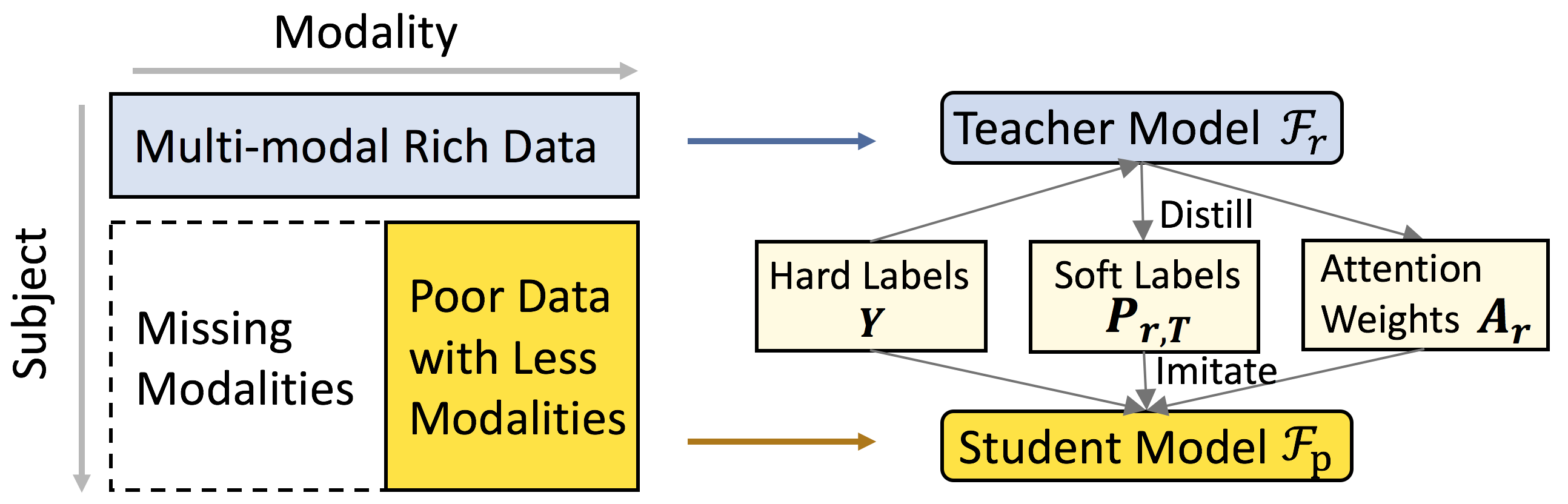
Figure 1: The framework of RDPD. Given teacher model along with attention weights learned from rich data, RDPD trains the student model on poor data while imitating the behavior and performance of teacher model. In particular, RDPD jointly optimize the combined loss of attention imitation (behavior) and target imitation (performance). The loss of target imitation also concerns both hard labels from data and soft labels provided by the teacher model.

Consider data collected via continuous time series, given a teacher model trained from rich data environment, we want to teach a student model running on only poor data. And we hope the student model could benefit from the information contained in rich data via the teacher model, by imitating the teacher model in terms of learning outcome and the learning process. In this work, we call the former objective as target imitation, and the latter one as behavior imitation. Target imitation can be achieved by imitating the final predictions (i.e., soft labels) of the teacher model while behavior imitation can be achieved by imitating its attention weights over temporal time series.

Mathematically, denote $\bm{X}_{r}$ as the multi-modal rich data with $D_{r}$ modalities that is available in training phase, and $\bm{X}_{p}$ as the poor data with $D_{p}$ modalities that is available in both training and testing phases. Here the modalities in $\bm{X}_{p}$ are a subset of $\bm{X}_{r}$, and $D_{p}<D_{r}$; $\bm{X}_{p}$ and $\bm{X}_{r}$ share the same labels $\bm{Y}$. Our task is to build a student model $\mathcal{F}_{p}$ which only takes $\bm{X}_{p}$ as input, and will benefit from knowledge transferred from $\bm{X}_{r}$.

Overview. For RDPD, the student model trained on poor data will imitate teacher model trained on rich data and hard labels in both intermediate learning behavior and final learning performance. The imitation of learning behavior is achieved by optimizing information loss from distribution of attention in student model to distribution of attention in teacher model while the performance imitation is done by jointly optimizing hard label, soft label and and their trainable combination. In the following we will detail each step of RDPD.

2.2 Training Teacher Model

Although RDPD can be applied on time series in general, in this paper we only consider regularly sampled continuous time series $\bm{X_{r}}$ (e.g., sensor data). Assume a patient has time series from $D_{r}$ modalities, for time series in each modality with length $l$, we split $\bm{X_{r}}\in\mathbb{R}^{l\times D_{r}}$ into $M$ segments at length $S$, thus $l=M\times S$. We denote multi-modal segmented input time series as $\bm{S_{r}}\in\mathbb{R}^{M\times S\times D_{r}}$.

We applied stacked 1-D convolutional neural networks (CNN) on each segment and recurrent neural networks (RNN) across segments. Such a design has been demonstrated to be effective in many previous studies on multivariate time series modeling  Ordóñez and Roggen (2016); Choi et al. (2016). In detail, we apply 1-D CNN with mean pooling on each segment $\bm{s_{r}}^{(j)}\in\mathbb{R}^{S\times D_{r}},j=1,\cdots,M$ as given by Eq. 1. Parameters including number of filters, filter size and stride in CNN are shared among segments $\bm{s_{r}}^{(1)},\cdots,\bm{s_{r}}^{(M)}$, and vary across different datasets. Details are shown in the Experiment Setup section.

$$\bm{h_{r}}^{(j)}=Pooling(CNN_{1D}(\bm{s_{r}}^{(j)}))$$ (1)

Then, we concatenate all convolved and pooled segments to get $\bm{H_{r}}=[\bm{h_{r}}^{(1)},\cdots,\bm{h_{r}}^{(M)}]^{T}\in\mathbb{R}^{M\times K_{r}}$, where $K_{r}$ is the number of filters in $CNN_{1D}$. Next we applied an RNN layer on $\bm{H_{r}}$ and denote the output as $\bm{Q_{r}}$ such that $\bm{Q_{r}}=RNN(\bm{H_{r}})$. And $\bm{Q_{r}}\in\mathbb{R}^{M\times U_{r}}$, where $U_{r}$ is the number of hidden units in RNN layer. Here we use the widely-applied self-attention mechanism  Lin et al. (2017) as it is a natural choice to get better results by taking advantage of the correlations or importance of segments. It also generates attention weights $\bm{A_{r}}$ that could represent teacher’s behaviors on each segment. The attention weights are calculated by Eq. 2.

$$\bm{A_{r}}=softmax(\bm{Q_{r}}\bm{W})$$ (2)

where $\bm{W}\in\mathbb{R}^{U_{r}\times 1}$, $\bm{A_{r}}\in\mathbb{R}^{M\times 1}$. We then multiplied the RNN output $\bm{Q_{r}}$ with corresponding attention weights $\bm{A_{r}}$. The weighted output $\bm{G_{r}}$ is given by Eq. 3.

$$\bm{G_{r}} = \bm{A_{r}}^{T}\bm{Q_{r}}$$ (3)

where $\bm{G_{r}}\in\mathbb{R}^{1\times U_{r}}$. Finally, the weighted output $\bm{G_{r}}$ is further transformed by a dense layer with weights $\bm{W_{d}}\in\mathbb{R}^{U_{r}\times C}$ to output logits $\bm{O_{r}}\in\mathbb{R}^{1\times C}$.

$$\bm{O_{r}} = \bm{G_{r}}\bm{W_{d}}$$ (4)

For simplicity, we can summarize from Eq.1 to Eq.4 to represent the teacher model $\mathcal{F}_{r}$ as in Eq. 5: $\mathcal{F}_{r}$ takes $\bm{X_{r}}$ as inputs and outputs logits $\bm{O_{r}}$ and attention weights $\bm{A_{r}}$.

$$\mathcal{F}_{r}(\bm{X_{r}}) = \bm{A_{r}},\bm{O_{r}}$$ (5)

The objective function of the teacher model measures prediction accuracy, and also provides knowledge to student model. Typically, $\bm{O_{r}}$ are transformed by softmax as final predicted probabilities, which can be used as distilled knowledge for student model to imitate. However, sharp distribution (e.g, hard labels) will be less informative. To alleviate this issue, we follow the idea in  Hinton et al. (2015) to produce more informative soft labels. Compared with hard label, the soft label imitation has much smoother probability distribution over classes, thus contains richer (larger entropy) informations. Concretely, we modify classic softmax to $\mathcal{S}(x,T)$ by dividing original logits $\bm{O_{r}}$ with a predefined hyper-parameter $T$ (larger than 1). $T$ is usually referred to as Temperature. The modified softmax (shows $i$th soft probability) is given by Eq. 6 and the soft predictions are given by Eq. 7.

$$\mathcal{S}(\bm{x},T)_{i} =\frac{\exp(x_{i}/T)}{\sum_{j}\exp(x_{j}/T)}$$ (6)

$$\bm{P_{r,T}} =\mathcal{S}(\bm{O_{r}},T)$$ (7)

Finally, we use cross-entropy loss as prediction loss $\mathcal{L}_{teacher}$ (in Eq. 8) to measure the difference between soft predictions $\bm{P_{r,T}}\in\mathbb{R}^{1\times C}$ and ground truth $\bm{Y}\in\mathbb{R}^{1\times C}$. We optimize teacher model via minimizing $\mathcal{L}_{teacher}$.

$$\mathcal{L}_{teacher}=CrossEntropy(\bm{Y},\bm{P_{r,T}})$$ (8)

2.3 Imitating Attentions and Targets

After training teacher model on rich data, we now describe the imitation process for the student model. For attention imitation, we mean to mimic attention weights. For target imitation, the student model imitates the following components: 1) soft label that is more informative, 2) hard label that could improve performance (according to  Hinton et al. (2015)), and 3) a trainable combination of both soft label and hard label. Again, we start with constructing the student model $\mathcal{F}_{p}$ using a CNN + RNN architecture, but with fewer filters in CNN and fewer hidden units in RNN. In our experiment, we roughly keep the proportion of hyper-parameters in teacher model to student model the same as the proportion of $D_{r}$ to $D_{p}$ using $K_{r}/K_{p}\approx D_{r}/D_{p}$, where $K_{r}$ and $K_{p}$ is the number of filters of CNN in teacher model and student model. Also, $U_{r}/U_{p}\approx D_{r}/D_{p}$, where $U_{r}$ and $U_{p}$ is the number of hidden units of RNN in teacher model and student model. Similar to Eq.5, $\mathcal{F}_{p}$ takes $\bm{X_{p}}$ as inputs and outputs logits $\bm{O_{p}}$ and attention weights $\bm{A_{p}}$ as in Eq. 9.

$$\mathcal{F}_{p}(\bm{X_{p}}) = \bm{A_{p}},\bm{O_{p}}$$ (9)

2.3.1 Attention Imitation

In Eq.2 we define attention weights to represent the influence of different time segments to the final predictions. We assume that the attention behavior of student model should resemble that of teacher model, and formulate the attention imitation as below. Given Eq.5 and Eq.9, to enforce $\bm{A_{p}}$ and $\bm{A_{r}}$ to have similar distributions, we minimize the Kullback-Leibler (KL) divergence $\mathcal{L}_{att}$ given by Eq. 10 to measure the information loss from distribution of attention in student model $\bm{A_{p}}$ to distribution of attention in teacher model $\bm{A_{r}}$.

$$\mathcal{L}_{att} = D_{KL}(\bm{A_{p}}||\bm{A_{r}})$$ (10)

2.3.2 Imitating Hard Labels

For hard label imitation, we optimize the student model by minimizing cross entropy loss $\mathcal{L}_{hard}$ (in Eq. 11) that measures the difference between predicted target values and ground truth values $\bm{Y}\in\mathbb{R}^{1\times C}$, where $C$ is the number of target classes, $\bm{P_{p,1}}=\mathcal{S}(\bm{O_{p}},1)$.

$$\mathcal{L}_{hard}=CrossEntropy(\bm{Y},\bm{P_{p,1}}),$$ (11)

2.3.3 Imitating Soft Labels

Given soft labels from $\mathcal{F}_{r}$, we produce soft predictions $\bm{P_{p,T}}$ by the same temperature $T$ on softmax in student model $\mathcal{F}_{p}$. Then, we optimize a cross entropy loss $\mathcal{L}_{soft}$ (in Eq. 12) that measures the differences between student and teacher.

$$\mathcal{L}_{soft}=T^{2}CrossEntropy(\bm{P_{r,T}},\bm{P_{p,T}})$$ (12)

Here, $\bm{P_{r,T}}$ is defined in Eq.7. $\bm{P_{p,T}}=\mathcal{S}(\bm{O_{p}},T)$. Since the magnitudes of gradients in Eq.12 is scaled by $1/T^{2}$ as we divided logits by $T$, we should multiply the soft imitation loss by $T^{2}$ to keep comparable gradient during implementation.

2.3.4 Imitating Combined Label

While hard labels provide certain prediction outcomes and soft labels provide probabilistic predictions, the two labels may even be opposite. To resolve the gap between the two labels, a reasonable solution is to combine them to yield uncertain prediction (probabilities of each class). Besides, while hard label imitation helps student model learn more information from data, soft label imitation transfer more knowledge from the teacher model (smoother distribution), each will lead to either more bias (comes from data) or more variance (comes from model). To leverage their benefits and make them complement each other, we propose to minimize a linear combination of hard labels and soft labels, denoted as $\bm{P_{p,comb}}$ as the follows:

$$\bm{P_{p,comb}}=\mathcal{S}(w_{1}\bm{P_{p,1}}+w_{2}\bm{P_{p,T}}+b,1)$$ (13)

where $w_{1},w_{2},b$ are learnable parameters. For the combined imitation, we also use cross entropy loss $\mathcal{L}_{comb}$ (in Eq. 14) to define the loss between $\bm{P_{p,comb}}$ and ground truth $\bm{Y}$.

$$\mathcal{L}_{comb}=CrossEntropy(\bm{Y},\bm{P_{p,comb}})$$ (14)

2.4 Joint Optimization

Finally, for the student model to imitate attentions and targets simultaneously, we jointly optimize all loss functions above. Here, we simply summed them up to get the final objective function $\mathcal{L}_{student}$ given by Eq. 15. We summarize the RDPD method in Algorithm 1.

$$\mathcal{L}_{student}=\mathcal{L}_{att}+\mathcal{L}_{hard}+\mathcal{L}_{soft}+\mathcal{L}_{comb}$$ (15)

Algorithm 1 RDPD ($\bm{X_{r}},\bm{X_{p}},\bm{Y},T$)

1:  Build teacher model $\mathcal{F}_{r}$

2:  Compute $\bm{A_{r}},\bm{O_{r}}=\mathcal{F}_{r}(\bm{X_{r}})$

3:      $\bm{P_{r,T}}=\mathcal{S}(\bm{O_{r}},T)$

4:      $\mathcal{L}_{teacher}=CrossEntropy(\bm{Y},\bm{P_{r,T}})$

5:  while not convergence do

6:     Update weights of $\mathcal{F}_{r}$ by optimizing $\mathcal{L}_{teacher}$ using back-propagation

7:  end while

8:  Build student model $\mathcal{F}_{p}$

9:  Compute $\bm{A_{p}},\bm{O_{p}}=\mathcal{F}_{p}(\bm{X_{p}})$

10:      $\bm{P_{p,T}}=\mathcal{S}(\bm{O_{p}},T)$, $\bm{P_{p,1}}=\mathcal{S}(\bm{O_{p}},1)$

11:      $\bm{P_{p,comb}}=\mathcal{S}(w_{1}\bm{P_{p,1}}+w_{2}\bm{P_{p,T}}+b,1)$

12:      $\mathcal{L}_{att}=D_{KL}(\bm{A_{p}}||\bm{A_{r}})$

13:      $\mathcal{L}_{hard}=CrossEntropy(\bm{Y},\bm{P_{p,1}})$

14:      $\mathcal{L}_{soft}=T^{2}CrossEntropy(\bm{P_{r,T}},\bm{P_{p,T}})$

15:      $\mathcal{L}_{comb}=CrossEntropy(\bm{Y},\bm{P_{p,comb}})$

16:      $\mathcal{L}_{student}=\mathcal{L}_{att}+\mathcal{L}_{hard}+\mathcal{L}_{soft}+\mathcal{L}_{comb}$

17:  while not convergence do

18:     Update weights of $\mathcal{F}_{p}$ by optimizing $\mathcal{L}_{student}$ using back-propagation

19:  end while

3 Experiments

3.1 Experiment Setup

3.1.1 Datasets

We used the following datasets in performance evaluation. Data statistics are summarized in Table 1.

PAMAP2 Physical Activity Monitoring Data Set (PAMAP2)

Reiss and Stricker (2012) contains 52 channels of sensor signals of 9 subjects wearing 3 inertial measurement units (IMU, 100Hz) and a heart rate monitor (HR, 9Hz). The average length of each subject is about 42k points. We down-sample the signals to 50 Hz and choose $S=64$ for experiment. We followed the “frame-by-frame analysis” in Reiss and Stricker (2012) to pre-process the time series with sliding windows of 5.12 seconds duration and 1 second stepping between adjacent windows. The task is to classify signals into one of the $12$ different physical activities (e.g., walking, running, standing, etc.). In our experiment, we choose data of subject 105 for validation, subject 101 for testing, and others for training.

The PTB Diagnostic ECG Database (PTBDB)

includes 15 channels of ECG signals collected from controls and patients of heart diseases  Bousseljot et al. (1995). The database contains 549 records from 290 subjects. We down-sample the signals to 200 Hz and choose $S=500$ for experiment. Similar to PAMAP2, we pre-processed the data using “frame-by-frame analysis” with sliding windows of 10 seconds duration and 5 second stepping between adjacent windows. Our task is to classify signals into one of the 6 patient groups. In our experiment, we random divided the data into training (80%), validation (10%) and test (10%) sets by subjects.

The Medical Information Mart for Intensive Care (MIMIC-III)

is collected on over $58,000$ ICU patients at the Beth Israel Deaconess Medical Center (BIDMC) from June 2001 to October 2012  Johnson et al. (2016). In our experiment, we focus on patients with following diseases: 1) acute myocardial infarction, 2) chronic ischemic heart disease, 3) heart failure, 4) intracerebral hemorrhage, 5) specified procedures complications, 6) lung diseases,7) endocardium diseases, and 8) septicaemia, in total $9,488$ subjects. In detail, we extract 6 vital sign time series of the first 48 hours including heart rate (HR), Respiratory Rate (RR), Blood Pressure mean, Blood Pressure systolic, Blood Pressure diastolic and SpO2. We resample the time series to 1 point per hour and choose $S=12$ for experiment. Our task is to classify vital sign series into one of the 8 diseases. In our experiment, we random divided the data into training (80%), validation (10%) and test (10%) sets by patients.

	PAMAP2	PTBDB	MIMIC-III
# subjects	9	290	9,488
# classes	12	6	8
# attributes	52	15	6
Total time series length	2,872,533	59,619,455	455,424
Sample Frequency	100 Hz (IMU)	1,000 Hz	1 per hour
	9 Hz (HR)

Table 1: Statistics of Datasets

3.1.2 Evaluations and Implementation Details

Performance was measured by the Area under the Receiver Operating Characteristic (ROC-AUC), Area under the Precision-Recall Curve (PR-AUC), and macro F1 score (macro-F1). ROC-AUC and PR-AUC are evaluated between predicted probabilities and ground truth. The PR-AUC is considered a better measure for imbalanced data with much more negative samples like our setting Davis and Goadrich (2006). Macro-F1 is a commonly used with threshold $0.5$, which determine whether a given probability is predicted as $1$ (larger than threshold) or $0$ (smaller than threshold).

Models are trained with the mini-batch of 128 samples for 200 iterations, which was a sufficient number of iterations for achieving the best performance for the classification task. The final model was selected using early stopping criteria on validation set. We then tested each model for 10 times using different random seeds, and report their mean values with standard deviation. All models were implemented in PyTorch version 0.5.0., and trained with a system equipped with 64GB RAM, 12 Intel Core i7-6850K 3.60GHz CPUs and Nvidia GeForce GTX 1080. All models were optimized using Adam  Kingma and Ba (2014), with the learning rate set to 0.001. Our code is publicly available at https://github.com/hsd1503/RDPD.

3.1.3 Comparative Methods

We will compare following methods:

• Teacher: Teacher model is trained and tested on all channels. The model has better accuracy, a much heavier model architecture, and is only available for in-hospital setting where all channels of signals are available. It serves as an empirical upper bound of performance.

• Direct: Direct model is build on the partially observed data using RCNN, without attention imitation and soft label imitation. This model is equivalent to $\mathcal{L}=\mathcal{L}_{hard}$.

• Knowledge Distillation (KD): KD  Hinton et al. (2015) model is constructed on the partially observed data, with soft label imitation and hard label imitation. This model is equivalent to $\mathcal{L}=\mathcal{L}_{hard}+\mathcal{L}_{soft}$.

• Ours including $\texttt{RDPD}_{\bm{r1}}$: The reduced version of RDPD without attention imitation. And the objective function would be $\mathcal{L}=\mathcal{L}_{comb}+\mathcal{L}_{hard}+\mathcal{L}_{soft}$. $\texttt{RDPD}_{\bm{r2}}$: The reduced version of RDPD without combined labels. This model is equivalent to KD model with attention imitation. And the objective function would be $\mathcal{L}=\mathcal{L}_{att}+\mathcal{L}_{hard}+\mathcal{L}_{soft}$. RDPD: Our whole model contains all proposed imitations. Using $\mathcal{L}=\mathcal{L}_{att}+\mathcal{L}_{hard}+\mathcal{L}_{soft}+\mathcal{L}_{comb}$ as objective function.

For all models, we use 1 layer 1-D CNN and 1 layer Bi-directional LSTM. In teacher model, for PAMAP2, the number of filters is set to 64, filter size is set to 8, stride is set to 4 and the number of hidden units is set to 32. For PTBDB, they are set to 128, 32, 8, 32 respectively. For MIMIC-III, they are set to 64, 4, 2, 32 respectively. In RDPD and compared baselines, since they have less input modalities, they have smaller number of CNN filters and RNN hidden units which is set proportionally as introduced before. However, the data length remains the same, so their filter size and stride keep unchanged. $T$ is set to 5 for PAMAP2 and PTBDB, and set to 2.5 for MIMIC-III.

3.2 Results

3.2.1 Classification Performance

We compared the results of RDPD against other baselines and the reduced version of RDPD in Table 2 (PAMAP2 dataset), Table 3 (PTBDB dataset) and Table 4 (MIMIC-III dataset). RDPD outperformed other methods (except Teacher) in most cases and demonstrated the proposed attention imitation and target imitation successfully improved performance of student model. The teacher model performs best among all methods since it is trained using a full datasets with multiple modalities. It serves an empirical upper bound of the performance. In Table 3, RDPD works better than its reduced version in PR-AUC and F1-score but not ROC-AUC. The reason is that classes in PTBDB dataset is very imbalanced, some occasional samples in rare classes distort the final result.

Data	Method	ROC-AUC	PR-AUC	macro-F1
All	Teacher	0.928 $\pm$ 0.014	0.708 $\pm$ 0.039	0.608 $\pm$ 0.045
Wrist	Direct	0.800 $\pm$ 0.032	0.452 $\pm$ 0.051	0.376 $\pm$ 0.049
	Distill	0.825 $\pm$ 0.020	0.469 $\pm$ 0.052	0.380 $\pm$ 0.060
	$\texttt{RDPD}_{r1}$	0.837 $\pm$ 0.025	0.491 $\pm$ 0.037	0.406 $\pm$ 0.053
	$\texttt{RDPD}_{r2}$	0.836 $\pm$ 0.018	0.478 $\pm$ 0.038	0.401 $\pm$ 0.049
RDPD	0.838 $\pm$ 0.012	0.491 $\pm$ 0.045	0.425 $\pm$ 0.057
Chest	Direct	0.836 $\pm$ 0.035	0.519 $\pm$ 0.065	0.449 $\pm$ 0.069
	Distill	0.868 $\pm$ 0.025	0.575 $\pm$ 0.043	0.486 $\pm$ 0.065
	$\texttt{RDPD}_{r1}$	0.872 $\pm$ 0.028	0.605 $\pm$ 0.030	0.518 $\pm$ 0.037
	$\texttt{RDPD}_{r2}$	0.879 $\pm$ 0.027	0.600 $\pm$ 0.051	0.478 $\pm$ 0.048
RDPD	0.883 $\pm$ 0.016	0.609 $\pm$ 0.052	0.529 $\pm$ 0.051
Ankle	Direct	0.811 $\pm$ 0.035	0.513 $\pm$ 0.065	0.405 $\pm$ 0.080
	Distill	0.901 $\pm$ 0.015	0.621 $\pm$ 0.044	0.492 $\pm$ 0.070
	$\texttt{RDPD}_{r1}$	0.889 $\pm$ 0.021	0.581 $\pm$ 0.071	0.443 $\pm$ 0.095
	$\texttt{RDPD}_{r2}$	0.904 $\pm$ 0.019	0.629 $\pm$ 0.041	0.473 $\pm$ 0.069
RDPD	0.910 $\pm$ 0.014	0.639 $\pm$ 0.030	0.511 $\pm$ 0.033

Table 2: Performance comparison on PAMAP2 dataset. The task is multi-class classification (12 classes). All contains 52 channels, Wrist contains 17 channels signals of 1 IMU over the wrist on the dominant arm, Chest contains 17 channels signals of 1 IMU on the chest, Ankle contains 17 channels signals of 1 IMU on the dominant side’s ankle.

Data	Method	ROC-AUC	PR-AUC	macro-F1
All	Teacher	0.737 $\pm$ 0.035	0.293 $\pm$ 0.018	0.288 $\pm$ 0.028
Lead I	Direct	0.701 $\pm$ 0.023	0.279 $\pm$ 0.017	0.164 $\pm$ 0.020
	Distill	0.676 $\pm$ 0.045	0.282 $\pm$ 0.022	0.217 $\pm$ 0.016
	$\texttt{RDPD}_{r1}$	0.677 $\pm$ 0.036	0.255 $\pm$ 0.029	0.139 $\pm$ 0.027
	$\texttt{RDPD}_{r2}$	0.707 $\pm$ 0.073	0.282 $\pm$ 0.044	0.218 $\pm$ 0.024
RDPD	0.706 $\pm$ 0.075	0.293 $\pm$ 0.025	0.218 $\pm$ 0.019

Table 3: Performance comparison on PTBDB dataset. The task is multi-class classification (6 classes). All contains 15 channels of ECG signals. Lead I contains single channel Lead I ECG signal, which is usually generated by mobile devices.

Data	Method	ROC-AUC	PR-AUC	macro-F1
All	Teacher	0.696 $\pm$ 0.011	0.281 $\pm$ 0.009	0.256 $\pm$ 0.012
BP	Direct	0.610 $\pm$ 0.016	0.204 $\pm$ 0.011	0.149 $\pm$ 0.013
	Distill	0.611 $\pm$ 0.013	0.206 $\pm$ 0.007	0.150 $\pm$ 0.005
	$\texttt{RDPD}_{r1}$	0.607 $\pm$ 0.012	0.203 $\pm$ 0.003	0.148 $\pm$ 0.003
	$\texttt{RDPD}_{r2}$	0.613 $\pm$ 0.020	0.205 $\pm$ 0.009	0.147 $\pm$ 0.007
RDPD	0.614 $\pm$ 0.018	0.207 $\pm$ 0.010	0.150 $\pm$ 0.006
HR	Direct	0.556 $\pm$ 0.019	0.176 $\pm$ 0.013	0.089 $\pm$ 0.042
	Distill	0.564 $\pm$ 0.021	0.175 $\pm$ 0.012	0.109 $\pm$ 0.030
	$\texttt{RDPD}_{r1}$	0.566 $\pm$ 0.010	0.178 $\pm$ 0.004	0.132 $\pm$ 0.005
	$\texttt{RDPD}_{r2}$	0.571 $\pm$ 0.011	0.176 $\pm$ 0.008	0.123 $\pm$ 0.016
RDPD	0.581 $\pm$ 0.014	0.182 $\pm$ 0.004	0.130 $\pm$ 0.010
RR	Direct	0.570 $\pm$ 0.019	0.176 $\pm$ 0.012	0.109 $\pm$ 0.039
	Distill	0.614 $\pm$ 0.023	0.201 $\pm$ 0.009	0.162 $\pm$ 0.015
	$\texttt{RDPD}_{r1}$	0.611 $\pm$ 0.014	0.202 $\pm$ 0.007	0.160 $\pm$ 0.016
	$\texttt{RDPD}_{r2}$	0.614 $\pm$ 0.017	0.205 $\pm$ 0.006	0.169 $\pm$ 0.010
RDPD	0.619 $\pm$ 0.022	0.207 $\pm$ 0.008	0.169 $\pm$ 0.007

Table 4: Performance comparison on MIMIC-III dataset. The task is multi-class classification (8 classes). All contains 6 channels of patient vital signs. BP contains blood pressure systolic and blood pressure diastolic, which is usually monitors by house sphygmomanometer. HR is heart rate, RR is respiration rate.

3.2.2 Reduction of Model Complexity

We analyzed model complexity by comparing model size of the teacher model and RDPD. Table 5 shows that the model size of RDPD is only $6-7\%$ of the model size of teacher model. According to experimental settings and previous results, other methods have comparable model size with our approach, but their performance are worse. In real world applications such as mobile health or ICU real-time modeling, it is very important that RDPD can achieve both lighter in model and better in performance.

Model	PAMAP2	PTBDB	MIMIC-III
Teacher	118.3k	335.0k	60.2k
RDPD	8.2k	19.8k	4.0k

Table 5: Model complexity comparison, the table shows number of parameters of each model.

3.2.3 Evaluation against Size of Rich Data

We evaluated the dependency of size of rich data. We used the same validation and test data, but scaled down the size of rich data in training. Figure 2 shows RDPD outperformed baselines even we have few rich data, and would perform better as we got more rich data. This demonstrated the efficacy of RDPD in extracting useful knowledge from rich data and teaching student even under rich-data insufficiency.

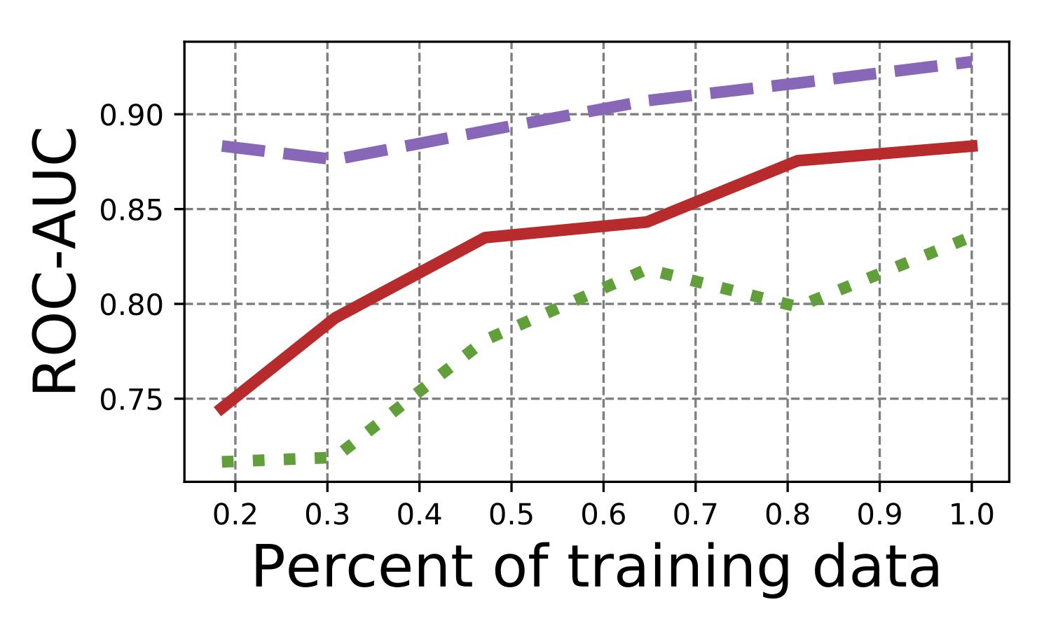
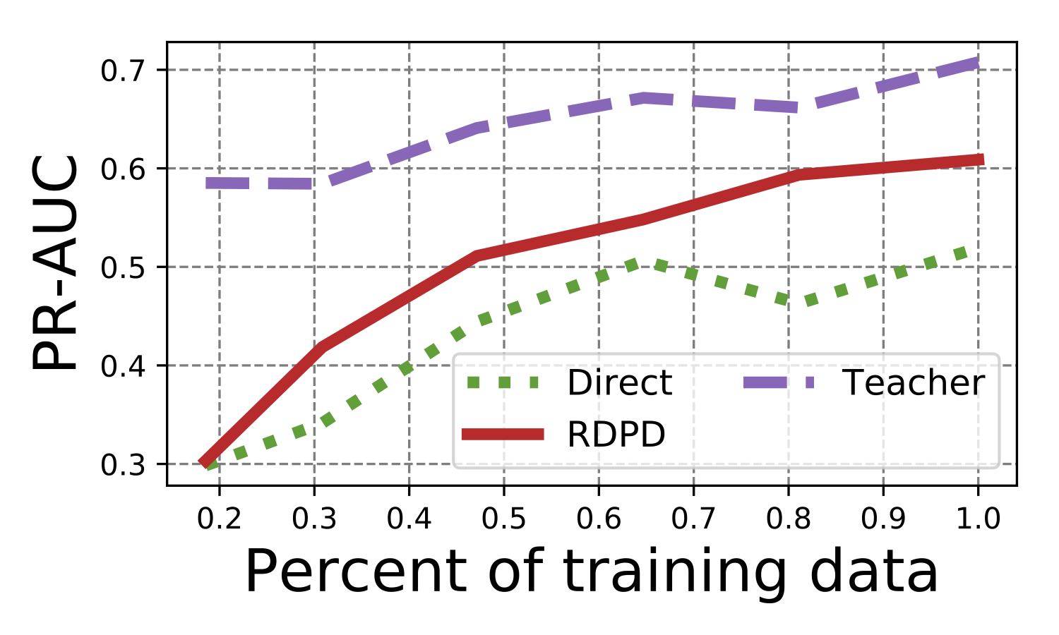
Figure 2: Performance comparison of training data size using PAMAP2 dataset.

3.2.4 Evaluation for the Setting of Low Quality Poor-data

Here we also assess how much benefit the multi-modality data can bring us from low quality poor-data. We performs experiments by adding different level of noise to the entire single modality. The approach of adding noise is: $\bm{x^{\prime}}=\bm{x}\oplus amp*random\_normal(-1,1)$, where $\bm{x}$ is the original data and $\bm{x^{\prime}}$ is the noise interfered data, $\oplus$ is element-wise add, $amp$ is the parameter to control the noise amplitude. From Figure 3, we can see with the increasing amplitude of noise, the performance of both Direct and RDPD decrease. However, RDPD still works better than Direct due to knowledge transfer from Teacher model.

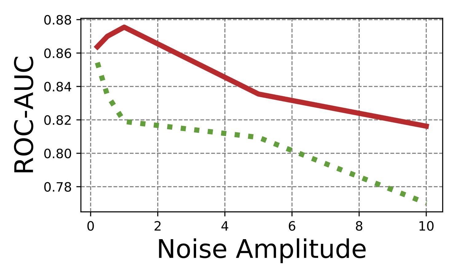
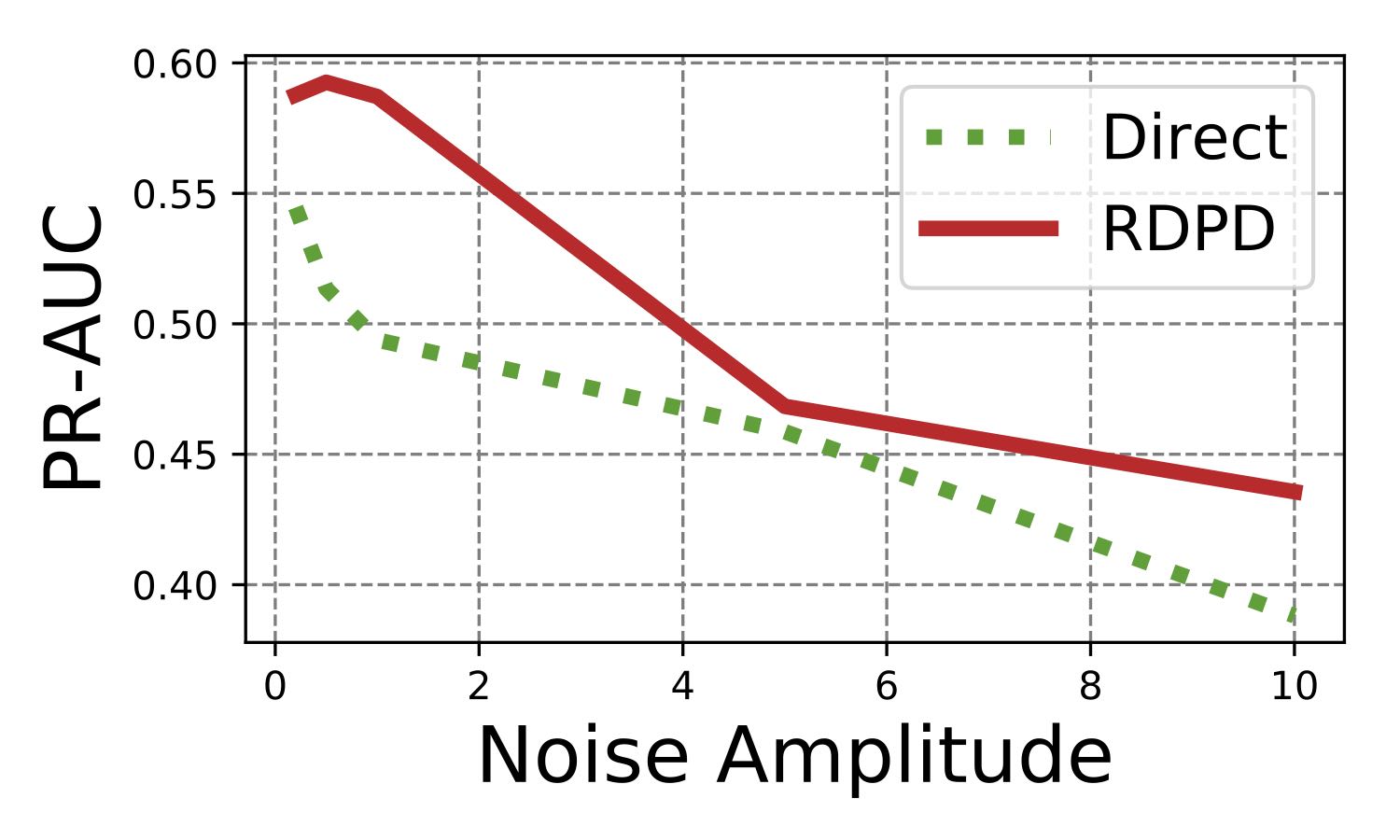
Figure 3: Performance comparison of noise amplitude using PAMAP2 dataset.

4 Related Work

Domain adaptation

Domain adaptation techniques address the problem of learning models on some source data distribution that generalize to a different target distribution. Deep learning based domain ad aptation methods have focused mainly on learning domain-invariant representations. For example,  Glorot et al. (2011) and  Chen et al. (2012) stacked Denoising Auto-encoders (SDA) and marginalized SDA respectively to extract meaningful representations.  Ganin et al. (2016) added a Gradient Reversal Layer that hinders the model’s ability to discriminate between domains. Moreover,  Zhou et al. (2016) transferred the source examples to the target domain and vice versa using BiTransferring Deep Neural Networks, while  Bousmalis et al. (2016) propose Domain Separation Networks. However they need to be trained jointly on source and target domain data and are therefore unappealing to the settings where both data are available.

Knowledge Distillation

Knowledge Distillation  Hinton et al. (2015) or mimic learning  Ba and Caruana (2014) are a family of approaches that aim to transfer the predictive power from more accurate deep models (“teacher model”) to smaller models (“student model”) like shallow neural networks  Hinton et al. (2015), soft decision tree  Frosst and Hinton (2017) via training smaller models on soft labels learned from deep models. It has been widely used in model compression  Sau and Balasubramanian (2016), omni-supervised learning  Radosavovic et al. (2017), fast optimization, network minimization and transfer learning  Yim et al. (2017). Extensions of knowledge distillation unifies distillation and privileged information into generalized distillation framework to learn from multiple machines and data representations  Lopez-Paz et al. (2015). The performance of distilled shallow neural networks are often better than models that are directly built on training data. The biggest difference between our approach and knowledge distillation is that, knowledge distillation focus on transfer powerful predictions ability of teacher to student model, while our approach is designed to transfer both behaviors and predictions from rich data modalities to poor data (a single modality).

Attention Transfer

Attention mechanism  Bahdanau et al. (2015) was proposed to improve performance of machine translation by paying more attention on relevant parts of the data. Recently, there are several works studying attention transfer  Zagoruyko and Komodakis (2017); Huang and Wang (2017) to enhance shallow neural networks. The goal was achieved by learning similar attention models in smaller neural networks, then defining attention as gradient with respect to the input  Zagoruyko and Komodakis (2017) or use regularization term  Huang and Wang (2017) to make two models have similar attention weights. Attention transfer has been used in video recognition from web images  Li et al. (2017), cross-domain sentiment classification  Li et al. (2018) and so on. The biggest difference between our approach and attention transfer is that attention transfer is used for model compression on one dataset, while our approach is used to transfer across datasets of very different data modalities.

5 Conclusion

In this paper we proposed to leverage the power of rich data to improve the learning from poor data with RDPD. RDPD learns end-to-end for the student model built on poor data to imitate the behavior (attention imitation) and performance (target imitation) of teacher model by jointly optimizing the combined loss of attention imitation and target imitation. We evaluated RDPD across multiple datasets and demonstrated its promising utility and efficacy. Future extension of RDPD includes considering modeling static meta information as one modality, and learning from less labels.

RDPD: Rich Data Helps Poor Data via Imitation

Appendix A Case Study

To further analyze the effects and reasons that how RDPD improves performance. We choose several subjects and compared their attention weights and prediction results learned by different methods.

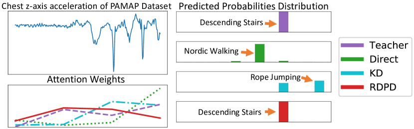
Figure 4: An example on PAMAP2 data.

Fig. 4 shows an example from PAMAP2. Both RDPD and Teacher correctly predict the subject is descending stairs, while Direct predicts the subject is doing Nordic walking and KD gives prediction of rope jumping. Fig. 4 left upper plots the z-axis acceleration from chest sensors, which shows the vertical acceleration of the whole body. Although these activities are similar, the change between walking on the floor and stairs distinguish the data from descending stairs with Nordic walking and rope jumping. Teacher model provide correct prediction by looking more channels, thus gives more attention in the vertical acceleration. RDPD also predicts correctly since it imitates the attentions from Teacher as shown in Figure 4 left bottom.

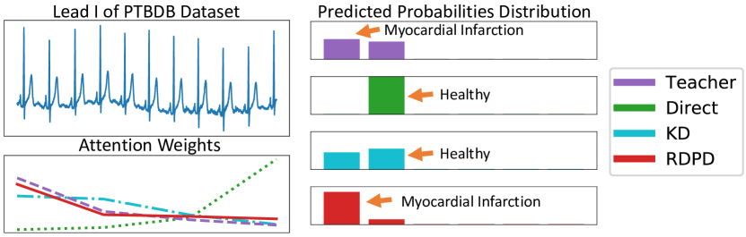
Figure 5: An example of PTBDB data and model predictions. (Left Upper) Original Lead I ECG data. (Left Bottom) Attention weights of different methods. (Right) Predicted probabilities distribution of different methods.

An example of PTBDB data and model predictions are shown in Figure 5. RDPD and Teacher give correct predictions while Direct and KD are wrong. The reason of RDPD better than KD and Direct comes from two aspects. One the one hand, RDPD and KD imitate Teacher’s soft label so that they correct wrong predictions like Direct in some extent. On the other hand, RDPD also imitate Teacher’s attention weights (shown in Left Bottom, purple is Teacher and red is RDPD), so that RDPD gives more confident predictions of Myocardial Infarction than KD, and thus further correct final predictions given by KD. Besides, we also found that RDPD gives more confident predictions of Myocardial Infarction than teacher model. The reason is that RDPD also considers combined label, and it leverages the soft label from Teacher model and hard label thus would be more confident when soft label and hard label are consistently right.

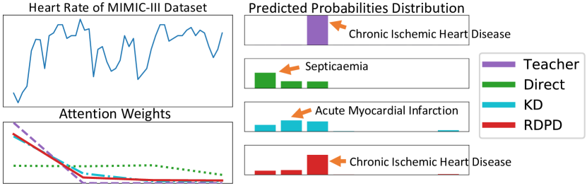
Figure 6: An example of MIMIC-III data and model predictions. (Left Upper) Original heart rate data. (Left Bottom) Attention weights of different methods. (Right) Predicted probabilities distribution of different methods.

An example of MIMIC-III data and model predictions are shown in Figure 6. RDPD and Teacher give correct predictions while Direct and KD are wrong. When looking at the attention weights (shown in left bottom), the Direct shows average weights on all part, while Teacher, KD and RDPD emphasize at the beginning. Moreover, in the first and the second part of attention weights, RDPD are in the middle of KD and Teacher, which reveal that RDPD successfully learns Teacher’s attentions that changes from KD to Teacher. In the right part, we can see that the probabilities of correct prediction increases from Direct to KD, and further increases in RDPD.

Appendix B Effect of Temperature

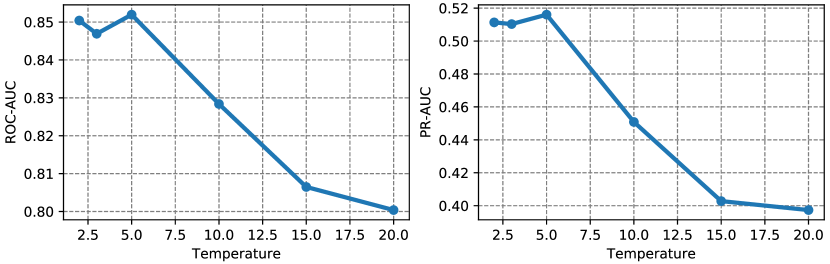
Figure 7: Performance comparison of temperature $T$ in RDPD on PAMAP2 dataset. (Left) ROC-AUC, (Right) PR-AUC.

Temperature $T$ is one critical hyperparameter that controls the degree of smoothness for soft labels. The larger of smoothing parameter $T$, the smoother of probability distribution over classes. To determine a proper value for $T$, our decision was based on the ROC-AUC and PR-AUC in validation set. In Figure 7 we plot the effects of hyperparameter $T$. It is easy to see that both ROC-AUC and PR-AUC slightly increase along the of $T$ from $1$ to $5$, then start to drop as $T$ becomes larger. The reason is that larger $T$ leads to a softer probabilities distribution, thus the model would be less discriminative and consequently yield lower ROC-AUC and PR-AUC. In our experiments, we set $T=5$ on PAMAP2 dataset as a proper choice.

References

- Ba and Caruana [2014] Jimmy Ba and Rich Caruana. Do deep nets really need to be deep? In Advances in neural information processing systems, pages 2654–2662, 2014.
- Bahdanau et al. [2015] Dzmitry Bahdanau, Kyunghyun Cho, and Yoshua Bengio. Neural machine translation by jointly learning to align and translate. ICLR, 2015.
- Bousmalis et al. [2016] Konstantinos Bousmalis, George Trigeorgis, Nathan Silberman, Dilip Krishnan, and Dumitru Erhan. Domain separation networks. In NIPS, pages 343–351, USA, 2016. Curran Associates Inc.
- Bousseljot et al. [1995] R Bousseljot, D Kreiseler, and A Schnabel. Nutzung der ekg-signaldatenbank cardiodat der ptb über das internet. Biomedizinische Technik/Biomedical Engineering, 40(s1):317–318, 1995.
- Chen et al. [2012] Minmin Chen, Zhixiang Xu, Kilian Q. Weinberger, and Fei Sha. Marginalized denoising autoencoders for domain adaptation. In ICML, pages 1627–1634, USA, 2012. Omnipress.
- Choi et al. [2016] Keunwoo Choi, George Fazekas, Mark Sandler, and Kyunghyun Cho. Convolutional recurrent neural networks for music classification. arXiv preprint arXiv:1609.04243, 2016.
- Davis and Goadrich [2006] Jesse Davis and Mark Goadrich. The relationship between precision-recall and roc curves. In Proceedings of the 23rd international conference on Machine learning, pages 233–240. ACM, 2006.
- Frosst and Hinton [2017] Nicholas Frosst and Geoffrey Hinton. Distilling a neural network into a soft decision tree. arXiv preprint arXiv:1711.09784, 2017.
- Ganin et al. [2016] Yaroslav Ganin, Evgeniya Ustinova, Hana Ajakan, Pascal Germain, Hugo Larochelle, François Laviolette, Mario Marchand, and Victor Lempitsky. Domain-adversarial training of neural networks. J. Mach. Learn. Res., 17(1):2096–2030, January 2016.
- Glorot et al. [2011] Xavier Glorot, Antoine Bordes, and Yoshua Bengio. Domain adaptation for large-scale sentiment classification: A deep learning approach. In ICML, pages 513–520, USA, 2011. Omnipress.
- Hinton et al. [2015] Geoffrey Hinton, Oriol Vinyals, and Jeff Dean. Distilling the knowledge in a neural network. arXiv preprint arXiv:1503.02531, 2015.
- Hong et al. [2017] Shenda Hong, Meng Wu, Yuxi Zhou, Qingyun Wang, Junyuan Shang, Hongyan Li, and Junqing Xie. ENCASE: an ENsemble ClASsifiEr for ECG Classification Using Expert Features and Deep Neural Networks. Computing in Cardiology, 44:1, 2017.
- Huang and Wang [2017] Zehao Huang and Naiyan Wang. Like what you like: Knowledge distill via neuron selectivity transfer. arXiv preprint arXiv:1707.01219, 2017.
- Johnson et al. [2016] Alistair EW Johnson, Tom J Pollard, Lu Shen, Li-wei H Lehman, Mengling Feng, Mohammad Ghassemi, Benjamin Moody, Peter Szolovits, Leo Anthony Celi, and Roger G Mark. Mimic-iii, a freely accessible critical care database. Scientific data, 3(1), 2016.
- Kingma and Ba [2014] Diederik Kingma and Jimmy Ba. Adam: A method for stochastic optimization. arXiv preprint arXiv:1412.6980, 2014.
- Li et al. [2017] Junnan Li, Yongkang Wong, Qi Zhao, and Mohan S Kankanhalli. Attention transfer from web images for video recognition. In Proceedings of the 2017 ACM on Multimedia Conference, pages 1–9. ACM, 2017.
- Li et al. [2018] Zheng Li, Ying Wei, Yu Zhang, and Qiang Yang. Hierarchical attention transfer network for cross-domain sentiment classification. In AAAI 2018, New Orleans, Lousiana, USA, February 2–7, 2018, 2018.
- Lin et al. [2017] Zhouhan Lin, Minwei Feng, Cicero Nogueira dos Santos, Mo Yu, Bing Xiang, Bowen Zhou, and Yoshua Bengio. A structured self-attentive sentence embedding. ICLR, 2017.
- Lopez-Paz et al. [2015] David Lopez-Paz, Léon Bottou, Bernhard Schölkopf, and Vladimir Vapnik. Unifying distillation and privileged information. ICLR, 2015.
- Ordóñez and Roggen [2016] Francisco Javier Ordóñez and Daniel Roggen. Deep convolutional and lstm recurrent neural networks for multimodal wearable activity recognition. Sensors, 16(1):115, 2016.
- Radosavovic et al. [2017] Ilija Radosavovic, Piotr Dollár, Ross Girshick, Georgia Gkioxari, and Kaiming He. Data distillation: Towards omni-supervised learning. arXiv preprint arXiv:1712.04440, 2017.