Closed string symmetries in open string field theory
– tachyon vacuum as sine-square deformation –

We revisit the identity-based solutions for tachyon condensation in open bosonic string field theory (SFT) from the viewpoint of the sine-square deformation (SSD). The string Hamiltonian derived from the simplest solution includes the sine-square factor, which is the same as that of an open system with SSD in the context of condensed matter physics. We show that the open string system with SSD or its generalization exhibits decoupling of the left and right moving modes and so it behaves like a system with a periodic boundary condition. With a method developed by Ishibashi and Tada, we construct pairs of Virasoro generators in this system, which represent symmetries for a closed string system. Moreover, we find that the modified BRST operator in the open SFT at the identity-based tachyon vacuum decomposes to holomorphic and antiholomorphic parts, and these reflect closed string symmetries in the open SFT. On the basis of SSD and these decomposed operators, we construct holomorphic and antiholomorphic continuous Virasoro algebras at the tachyon vacuum. These results imply that it is possible to formulate a pure closed string theory in terms of the open SFT at the identity-based tachyon vacuum.

1 Introduction

Open bosonic string field theories on a D-brane have a stable vacuum where a tachyon field is condensed and the D-brane disappears. At the tachyon vacuum, it is proved that we have no open strings as physical degrees of freedom and there is a belief that closed strings living in a bulk space-time are found. Since the on-shell closed string spectrum is obtained in a scattering amplitude in the perturbative vacuum of open string field theories, it is reasonable that there are some observables made by open string fields to clarify the existence of closed strings even on the tachyon vacuum. If it was realized, a pure closed string theory would be formulated in terms of open string fields.

In string theories, it has long been considered that closed string dynamics is described by open string degrees of freedom. It is naively intuitive that a closed string is given by a bound state of an open string and so an open string is regarded as a fundamental degree of freedom. This idea is realized in matrix theories, which are comprehensive or constructive theories including closed strings and D-branes, where matrices are considered as collections of zero modes of open strings. The AdS/CFT correspondence also provides a sophisticated version of this thought.

About a decade ago, Gendiar, Krcmar and Nishino made an important discovery concerning discretized open systems in condensed matter physics [1]. As an example, they considered an $N$-site system with open boundary condition described by the Hamiltonian

$$\hat{H}=-t\sum_{l=1}^{N-1}\sin^{2}\frac{l\pi}{N}\left(\hat{c}_{l}^{\dagger}\hat{c}_{l+1}+\hat{c}_{l+1}^{\dagger}\hat{c}_{l}\right),$$ (1.1)

where $\hat{c}_{l}$ denotes a spinless free fermion on a 1D lattice, which satisfies $\{\hat{c}_{l},\,\hat{c}_{l^{\prime}}^{\dagger}\}=\delta_{l,l^{\prime}}$. This is a deformed Hamiltonian of a uniform open system by the sine square factor. They found that this system is equivalent to a system with a periodic boundary condition by calculating the ground state energy and correlation functions numerically. This result suggests that a discretized closed system can be described by degrees of freedom of a discretized open system, and, considering the continuum limit, the above idea is realized in a 2D field theory.

After their seminal papers [1], the deformation such as (1.1) is called the sine-square deformation (SSD) and it has been actively studied. The above correspondence between the open and closed systems is understood as a result of the equivalence of the ground states of the SSD and uniform periodic systems [2], and after that it has been proved exactly [3]. The SSD has been extended to deformation with other suppression of boundary effects and the generalized SSD has been applied not only to the free fermion system but also to various models [1, 2, 3, 4, 5]. Moreover, SSD has also been studied in the context of a field theoretical description [6, 7, 8, 9, 10, 11, 12]. These studies strongly suggest the equivalence of an SSD system and a periodic system, and, from the string theoretical viewpoint, the possibility of closed string theories in terms of open strings.

Interestingly, it has been pointed out in [10] that there is an intimate relation between the SSD system and open string field theories. On the string field theoretical side, it is known that one of the identity-based tachyon vacuum solutions [13, 14] provides a kinetic operator corresponding to a string Hamiltonian at the tachyon vacuum [15]:

$$L^{\prime}=\frac{1}{2}L_{0}^{\prime}-\frac{1}{4}(L_{2}^{\prime}+L_{-2}^{\prime})+\frac{3}{2},$$ (1.2)

where $L_{n}^{\prime}$ is the twisted ghost Virasoro operator with the central charge 24. This operator can be rewritten by using the twisted ghost energy-momentum tensor $T^{\prime}(z)$:

$$L^{\prime}=\oint\frac{dz}{2\pi i}\frac{-1}{4z}\left(z^{2}-1\right)^{2}\left(T^{\prime}(z)-6\right).$$ (1.3)

If we change the variable to $z=\exp(i\theta)$, the weighting function in $L^{\prime}$ becomes $\sin^{2}\theta$ due to a Jacobian and a conformal factor from $T^{\prime}(z)$. Hence, the kinetic operator turns out to be related to an SSD Hamiltonian in conformal field theories [10].

The identity-based solution is constructed by an integration of some local operators along a half string and the identity string field. As a result, the theory expanded around the solution includes the modified BRST operator expressed as the integration of local operators on a worldsheet, which is a useful tool for investigating the corresponding vacuum. Actually, we can find the perturbative vacuum in the theory expanded around the identity-based tachyon vacuum solution with high precision by a level truncation scheme [16, 17, 18], although the vacuum energy is analytically calculated later [19, 20, 21]. This is a remarkable feature that has never been seen in wedge-based solutions [22, 23]. Furthermore, closed string amplitudes generated by a propagator on the identity-based tachyon vacuum have been formally discussed [24, 25] and then a vacuum loop amplitude generated by the propagator was numerically calculated [26].

These facts about SSD and string field theories (SFT) indicate that we are able to formulate a pure closed string theory in terms of open string fields and the identity-based tachyon vacuum solution. In this paper, motivated by this possibility, we will try to find closed string symmetries in the open string field theory at the identity-based tachyon vacuum. To do so, we will mainly use the technique developed in dipolar quantization of 2D conformal field theories [7, 8, 9, 10]. Consequently, we will obtain holomorphic and antiholomorphic continuous Virasoro operators that commute with the modified BRST operator on the identity-based tachyon vacuum. The existence of such Virasoro operators implies that open SFT on the identity-based tachyon vacuum provides some observables given by the worldsheet without boundaries, i.e., observables of closed string theories.

This paper is organized as follows. In section 2, we will discuss sine-square-like deformation (SSLD) of open string systems. With the help of the dipolar quantization technique, we will explain how left and right moving modes, which correlate in an open boundary system, become decoupled in the system with SSLD. Due to this decoupling, we can find left and right continuous Virasoro algebras, namely holomorphic and antiholomorphic parts of the Virasoro algebra. Here, we emphasize that this left-right decoupling is the most important ingredient for realizing the equivalence between the system with SSLD and that with a periodic boundary condition. In section 3, we will discuss closed string symmetries in open string field theories at the identity-based tachyon vacuum. After a brief review of the identity-based tachyon vacuum solution, we will show that the modified BRST operator decomposes to the holomorphic and antiholomorphic parts and that they are nilpotent and anticommute with each other. It will be shown that these correspond to the holomorphic and antiholomorphic parts of the BRST operator of a closed string. Next, we will construct the energy-momentum tensor and Virasoro operators at the tachyon vacuum, which are related to closed string symmetries in the open string field theory. It is noted that the energy-momentum tensor given in this section includes a new notion of frame-dependent operators, and it is not the twisted ghost operators that appeared previously. Then, we will discuss ghost operators and ghost number at the tachyon vacuum. In addition, we will comment on other types of identity-based tachyon vacuum solutions. In section 4, we will give concluding remarks. Details of calculations are provided in the appendices.

2 Sine-square-like deformations of an open string system

2.1 Decoupling of left and right moving modes

The Hamiltonian of an open string is given by

$$H_{\rm O}=\int_{C_{+}}\frac{dz}{2\pi i}\,zT(z)+\int_{C_{-}}\frac{dz}{2\pi i}\,zT(z),$$ (2.1)

where $T(z)$ is the energy-momentum tensor, $C_{+}$ ($C_{-}$) denotes a counterclockwise contour along a unit semicircle in a upper (lower) half plane. The end points of $C_{\pm}$, $z=\pm 1$, correspond to open string boundaries. The first and second terms correspond to Hamiltonians of the left and right moving modes respectively, but they do not commute with each other due to open boundary conditions on $T(z)$. Since the two contours $C_{+}$ and $C_{-}$ form a circle, the Hamiltonian is given by the zeroth component of the Virasoro operators $L_{n}$. Thus, we do not encounter antiholomorphic Virasoro operators in the open string system.

Here, we consider the deformation of (2.1) by introducing a weighting function $g(z)$:

$$H_{g}=H_{g}^{+}+H_{g}^{-},~{}~{}~{}~{}~{}~{}H_{g}^{\pm}=\int_{C_{\pm}}\frac{dz}{2\pi i}\,g(z)T(z),$$ (2.2)

where $g(z)$ is a holomorphic function satisfying $g(\pm 1)=\partial g(\pm 1)=0$ and $\left(g(1/z^{*})\right)^{*}=g(z)/z^{2}$ is imposed for the hermiticity of $H_{g}$. $H_{g}^{+}$ and $H_{g}^{-}$ are left and right moving modes of $H_{g}$. The simplest example of $g(z)$ is given by

$$g(z)=-\frac{1}{4z}(z^{2}-1)^{2}.$$ (2.3)

As mentioned in the introduction, if we change the variable to $z=\exp(i\theta)$, the weighting function in $H_{g}$ is changed to $z^{-1}g(z)=\sin^{2}\theta$. Hence, the deformed Hamiltonian (2.2) provides a sort of generalization of the SSD Hamiltonian. In this sense, we call it the sine-square-like deformation, or SSLD for short.

Since $T(z)$ in (2.2) is the same that as in (2.1), it is expanded by holomorphic Virasoro operators only:

$$T(z)=\sum_{n=-\infty}^{\infty}L_{n}z^{-n-2}.$$ (2.4)

By using this expansion form and the Virasoro algebra, we can obtain a commutation relation for $T(z)$ (appendix A):

$$[T(z),\,T(z^{\prime})]=-(\,T(z)+T(z^{\prime})\,)\,\partial\delta(z,z^{\prime})-\frac{c}{12}\partial^{3}\delta(z,z^{\prime}),$$ (2.5)

where $c$ is the central charge of $T(z)$ and the delta function $\delta(z,z^{\prime})=\sum_{n=-\infty}^{\infty}z^{-n}z^{\prime n-1}$ is normalized as [13]

$$\int_{C_{+}+C_{-}}\frac{dz}{2\pi i}\,\delta(z,z^{\prime})=1.$$ (2.6)

By using (2.5), we can calculate the commutation relation between $H_{g}^{+}$ and $H_{g}^{-}$. The important point is that surface terms appear in the calculation as a result of derivatives of the delta function and these terms include a singular factor $\delta(\pm 1,\pm 1)$. However, the singular surface terms turn out to vanish due to the factors $g(\pm 1)$ and $\partial g(\pm 1)$, which are set to zero in the definition of $H_{g}$. As a result, we find that $H_{g}^{+}$ commutes with $H_{g}^{-}$ (A.11) and then the deformed system is decomposed into left and right moving parts as in periodic systems. Accordingly, it is concluded that the deformed system described by $H_{g}$ corresponds not to an open string system, but to a closed string system, although the Hamiltonian is constructed by a single holomorphic energy-momentum tensor.

It should be noted that the zeros of $g(z)$ and $\partial g(z)$ at open string boundaries cause decoupling of the left and right moving sectors. This is the mechanism by which periodic properties are achieved in the SSLD system.

2.2 Example of string propagations

Equal-time contours generated by $H_{g}$ have been discussed by Ishibashi and Tada in [10]. However, they did not explicitly consider left and right moving modes. In this subsection, we will illustrate equal-time contours generated by the Hamiltonian for the simplest function (2.3) with a focus on the emergence of left and right moving sectors, although it corresponds to the $Z_{2}$-symmetric case in [10].

According to [10], we introduce the parameters, $t$ and $s$, into the worldsheet generated by $H_{g}$ for the function (2.3):

$$t+is=\int^{z}\frac{dz}{g(z)}=\frac{2}{z^{2}-1},$$ (2.7)

where $t$ denotes time and $s$ parametrizes a string at a certain time. If we introduce polar coordinates as $z=re^{i\theta}$, they can be expressed by the parameters $t$ and $s$ on the upper half plane (${\rm Im}\,z\geq 0$),

$$\theta = \left\{\begin{array}[]{ll}\displaystyle\frac{\pi}{4}+\frac{1}{2}\arctan\frac{s^{2}+2t+t^{2}}{2s}&(s<0)\\ &\\ \displaystyle\frac{3\pi}{4}+\frac{1}{2}\arctan\frac{s^{2}+2t+t^{2}}{2s}&(s>0),\end{array}\right.$$ (2.11)

$$r = \left(\frac{s^{2}+(t+2)^{2}}{s^{2}+t^{2}}\right)^{\frac{1}{4}},$$ (2.12)

and on the lower half plane (${\rm Im}\,z\leq 0$),

$$\theta = \left\{\begin{array}[]{ll}\displaystyle-\frac{\pi}{4}+\frac{1}{2}\arctan\frac{s^{2}+2t+t^{2}}{2s}&(s>0)\\ &\\ \displaystyle-\frac{3\pi}{4}+\frac{1}{2}\arctan\frac{s^{2}+2t+t^{2}}{2s}&(s<0),\end{array}\right.$$ (2.16)

$$r = \left(\frac{s^{2}+(t+2)^{2}}{s^{2}+t^{2}}\right)^{\frac{1}{4}}.$$ (2.17)

The contour at the time $t=-1$ is given by the unit circle $r=1$, in which $s$ is related to $\theta$ as $s=-\cot\theta$. As $\theta$ increases from $0\ (z=1)$ to $\pi\ (z=-1)$ on the upper half plane, $s$ increases from $-\infty$ to $\infty$. Similarly, on the lower half plane, $s$ increases from $-\infty$ to $\infty$ with increasing $\theta$ from $-\pi$ to $0$.

The upper half plane corresponds to the worldsheet swept by the left moving sector of a string. Equal-time contours can be depicted by using (2.11) and (2.12), in which $s$ runs from $-\infty$ to $\infty$ as in the case of $t=-1$. As the equal-time contour in Fig. 1 (a), the unit semicircle $C_{+}$ at $t=-1$ becomes larger as time increases, while the boundaries of a string do not propagate due to the zeros of $g(z)$. At $t=0$, the midpoint of the string goes to infinity. After that the midpoint splits into two points on the real axis, and then the contour shrinks to $z=\pm 1$ from the outside of $C_{+}$ as $t\rightarrow\infty$. As the time decreases from $t=-1$, the contour becomes smaller with fixed boundaries and, at $t=-2$, the string separates into two parts at the midpoint. As $t\rightarrow-\infty$, the contour shrinks to $z=\pm 1$ from the inside of $C_{+}$.

Similarly, we can illustrate equal-time contours for propagation of the right moving sector of a string by using (2.16) and (2.17). As in Fig. 1 (b), the resulting contours are given by rotating these of the upper half plane by $180^{\circ}$ around the origin of the $z$ plane.

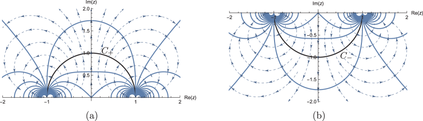
Figure 1: Equal-time contours on the $z$ plane (solid lines). Dashed lines with arrows denote evolution of time $t$.

These contours have a remarkable feature that the string boundaries are fixed at $z=\pm 1$ during propagation of the string. From (2.7), one complex number $t+is$ corresponds to two points in the $z$ plane. Accordingly, we introduce a complex coordinate $w=t+is$ for the upper half $z$ plane and $\bar{w}=t+is$ for the lower half plane. By this mapping, the upper half plane corresponds to the whole $w$ plane, and the lower half plane to the other $\bar{w}$ plane, as seen in Fig. 2.

Hence, the equal-time contours by $H_{g}$ lead us to the worldsheet that consists of two complex planes. The two planes, $w$ and $\bar{w}$, corresponding to the upper and lower half $z$ planes are generated by the left and right moving Hamiltonians, $H_{g}^{+}$ and $H_{g}^{-}$, respectively. Therefore, they can be regarded as holomorphic and antiholomorphic worldsheets of a closed string.

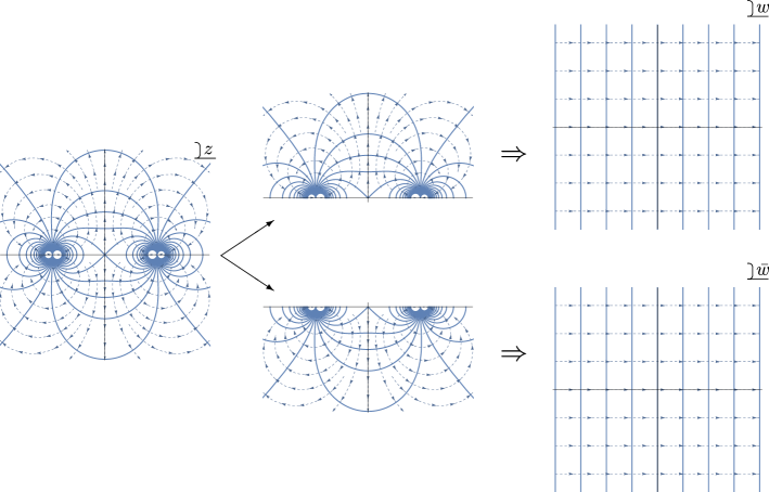
Figure 2: The equal-time contours generated by $H_{g}$ in the $z$ plane are divided into those of upper and lower half planes. By introducing the complex coordinates, $w$ and $\bar{w}$, the $z$ plane is mapped to two complex planes, which correspond to holomorphic and antiholomorphic parts for closed string worldsheets.

2.3 Virasoro algebra for closed strings

Now that we have obtained two decoupled Hamiltonians for the left and right moving sectors, we can construct two independent Virasoro operators according to [10]:

$${\cal L}_{\kappa}=\int_{C_{+}^{t}}\frac{dz}{2\pi i}g(z)f_{\kappa}(z)T(z),~{}~{}~{}~{}\tilde{\cal L}_{\kappa}=\int_{C_{-}^{t}}\frac{dz}{2\pi i}g(z)f_{\kappa}(z)T(z),$$ (2.18)

where $g(z)$ is the same function as that in the Hamiltonian (2.2) and $f_{\kappa}(z)$ is the function introduced in [10], which is defined by the differential equation

$$g(z)\frac{\partial}{\partial z}f_{\kappa}(z)=\kappa f_{\kappa}(z).$$ (2.19)

For a constant time $t$, $C_{+}^{t}$ and $C_{-}^{t}$ denote integral contours along the equal-time line on the upper and lower half $z$ plane, respectively. We should note again that $T(z)$ included in ${\cal L}_{\kappa}$ and $\tilde{\cal L}_{\kappa}$ is the same energy-momentum tensor of the open string system.

By setting $f_{\kappa=0}(z)=1$, ${\cal L}_{0}$ and $\tilde{\cal L}_{0}$ provide the left and right moving parts of the Hamiltonian (2.2), i.e., ${\cal L}_{0}=H_{g}^{+}$ and $\tilde{\cal L}_{0}=H_{g}^{-}$. ${\cal L}_{\kappa}$ satisfies the continuous Virasoro algebra

$$[{\cal L}_{\kappa},\,{\cal L}_{\kappa^{\prime}}] = (\kappa-\kappa^{\prime}){\cal L}_{\kappa+\kappa^{\prime}}$$ (2.20)

$$+\frac{c}{12}\int_{C_{+}^{t}}\frac{dz}{2\pi i}\left\{(\kappa-\kappa^{\prime})\left(\frac{\partial^{2}g}{\partial z^{2}}-\frac{1}{2g}\left(\frac{\partial g}{\partial z}\right)^{2}\right)+\frac{\kappa^{3}-{\kappa^{\prime}}^{3}}{2g}\right\}f_{\kappa+\kappa^{\prime}}(z),$$

which is antisymmetrized with respect to $\kappa$ and $\kappa^{\prime}$ compared to the equation given in [10]. Here, there is an important point in the derivation of (2.20), which was not mentioned in [10]. $g(z)$ in (2.2) has second- (or higher-) order zeros at the boundaries of $C_{\pm}^{t}$, $z=\pm 1$, where $f_{\kappa}(z)$ for $\kappa\neq 0$ has essential singularities, which follow from the differential equation (2.19). Accordingly, we need a regularization in addition to time-ordered products for evaluation of “equal-time” commutators.

We illustrate this point in the simplest case of (2.3). By solving the differential equation (2.19), we find

$$f_{\kappa}(z)=\exp\left(\frac{2\kappa}{z^{2}-1}\right),$$ (2.21)

where we impose $f_{0}(z)=1$. $f_{\kappa}(z)$ has essential singularities at $z=\pm 1$, which are second-order zeros of $g(z)$. In order to clarify the definition of ${\cal L}_{\kappa}$, we have to avoid these singularities on the integration paths. Here, we define ${\cal L}_{\kappa}$ by using an improper integral along a string at the time $t$:

$${\cal L}_{\kappa}=\lim_{s_{\rm max}\rightarrow\infty}\int_{C_{+}^{t,s_{\rm max}}}\frac{dz}{2\pi i}g(z)f_{\kappa}(z)T(z),$$ (2.22)

where $C_{+}^{t,s_{\rm max}}$ denotes the integration contour in which the parameter region of $s$, which is introduced in (2.7), is limited to $-s_{\rm max}\leq s\leq s_{\rm max}$. As usual, the “equal-time” commutator of ${\cal L}_{\kappa}$ and ${\cal L}_{\kappa^{\prime}}$ is regarded as a time-ordered product and so the commutator is calculated as

$$[{\cal L}_{\kappa},\,{\cal L}_{\kappa^{\prime}}] = \lim_{\begin{subarray}{c}\varDelta t\to+0\\ s_{\rm max}\to+\infty\end{subarray}}\int_{C_{+}^{t,s_{\rm max}}}\frac{dz^{\prime}}{2\pi i}g(z^{\prime})f_{\kappa^{\prime}}(z^{\prime})\times$$ (2.23)

$$\qquad\quad\times\left(\int_{C^{t+\varDelta t,s_{\rm max}}_{+}}-\int_{C^{t-\varDelta t,s_{\rm max}}_{+}}\right)\frac{dz}{2\pi i}\,g(z)f_{\kappa}(z)\,T(z)T(z^{\prime}).$$

We notice that, unlike the radial quantization, it is impossible to deform the integration paths of $z$ to a contour encircling $z^{\prime}$ since the paths have open boundaries associated with $\pm s_{\rm max}$. To derive (2.20) by the path deformation, we have to add the paths $C_{\pm 1}^{s_{\rm max}}$ as depicted in Fig. 3, in which $t$ varies from $t\mp\varDelta t$ to $t\pm\varDelta t$ with $s$ fixed to $\mp s_{\rm max}$.

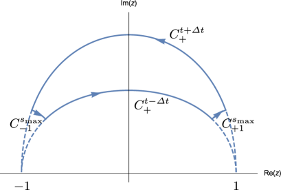
Figure 3: Regularization for the essential singularities

Then, what to be proved is that the integration along $C_{\pm 1}^{s_{\rm max}}$ becomes zero as $s_{\rm max}$ goes to infinity, i.e., as the paths shrink to the essential singularity points. Fortunately, it can be found that the limit of the integration is zero (see the discussion in appendix B) and the Virasoro algebra (2.20) holds for the operator defined as (2.22).

The right moving sector of the Virasoro operator $\tilde{\cal L}_{\kappa}$ should also be defined by avoiding singularities along the integration path on the lower half plane:

$$\tilde{\cal L}_{\kappa}=\lim_{s_{\rm max}\rightarrow\infty}\int_{C_{-}^{t,s_{\rm max}}}\frac{dz}{2\pi i}g(z)f_{\kappa}(z)T(z),$$ (2.24)

where $C_{-}^{t,s_{\rm max}}$ denotes the path in which the parameter region of $s$ is limited to $-s_{\rm max}\leq s\leq s_{\rm max}$. Similarly, $\tilde{\cal L}_{\kappa}$ satisfies the continuous Virasoro algebra. Moreover, since $C_{+}^{t,s_{\rm max}}$ and $C_{-}^{t,s_{\rm max}}$ have no intersections, ${\cal L}_{\kappa}$ and $\tilde{\cal L}_{\kappa}$ commute with each other under this regularization:

$$[{\cal L}_{\kappa},\,\tilde{\cal L}_{\kappa^{\prime}}]=0.$$ (2.25)

Thus, we have found two independent Virasoro algebras in a deformed open string system, which can be regarded as Virasoro algebras for closed strings, i.e., the holomorphic and antiholomorphic parts.

2.4 Natural frame for continuous Virasoro algebra

The continuous Virasoro algebra (2.20) is explicitly calculated for the simplest weighting function (2.3):

$$\big{[}{\cal L}_{\kappa},\,{\cal L}_{\kappa^{\prime}}\big{]} = (\kappa-\kappa^{\prime}){\cal L}_{\kappa+\kappa^{\prime}}+\frac{c}{12}\kappa^{3}\delta(\kappa+\kappa^{\prime})+\frac{3c}{96}(\kappa-\kappa^{\prime})(1+|\kappa+\kappa^{\prime}|)e^{-(\kappa+\kappa^{\prime}+|\kappa+\kappa^{\prime}|)},$$ (2.26)

$$\big{[}\tilde{\cal L}_{\kappa},\,\tilde{\cal L}_{\kappa^{\prime}}\big{]} = (\kappa-\kappa^{\prime})\tilde{\cal L}_{\kappa+\kappa^{\prime}}+\frac{c}{12}\kappa^{3}\delta(\kappa+\kappa^{\prime})+\frac{3c}{96}(\kappa-\kappa^{\prime})(1+|\kappa+\kappa^{\prime}|)e^{-(\kappa+\kappa^{\prime}+|\kappa+\kappa^{\prime}|)}.$$ (2.27)

The term $\frac{c}{12}\kappa^{3}\delta(\kappa+\kappa^{\prime})$ appears due to the last term in (2.20) proportional to $\kappa^{3}$ and this is also found in another example discussed in [10]. The third term in (2.26) or (2.27) is characteristic in this weighting function. But, it can be absorbed in a shift of ${\cal L}_{\kappa}$, since it is given as $\kappa-\kappa^{\prime}$ times a function of $\kappa+\kappa^{\prime}$.

We consider this shift of ${\cal L}_{\kappa}$ in the context of conformal transformation. As discussed in §2.2, we can introduce a complex coordinate in the upper half plane, $w=t+is$, which transforms the upper half $z$ plane to the whole $w$ plane. Now, in the $w$ plane, we define a Virasoro operator associated with ${\cal L}_{\kappa}$:

$$\hat{\cal L}_{\kappa}=\int_{\hat{C}_{+}^{t}}\frac{dw}{2\pi i}e^{\kappa w}T(w),$$ (2.28)

where $\hat{C}_{+}^{t}$ is an image of $C_{+}^{t}$ by the conformal transformation, which is the path from $t-i\infty$ to $t+i\infty$ parallel to the imaginary axis. By the conformal transformation, $\hat{\cal L}_{\kappa}$ is related to ${\cal L}_{\kappa}$ as

$$\hat{\cal L}_{\kappa}={\cal L}_{\kappa}-\frac{c}{12}\int_{C_{+}^{t}}\frac{dz}{2\pi i}g(z)f_{\kappa}(z)\{w,\,z\},$$ (2.29)

where $\{w,\,z\}$ is the Schwarzian derivative and, by using $dz/dw=g(z)$, it is calculated as

$$\{w,\,z\}=\frac{1}{g}\left(\frac{1}{2g}\left(\frac{\partial g}{\partial z}\right)^{2}-\frac{\partial^{2}g}{\partial z^{2}}\right).$$ (2.30)

We notice that this term is included in (2.20) as the term proportional to $\kappa-\kappa^{\prime}$ and so the shift (2.29) cancels this term in the continuous Virasoro algebra. Consequently, we can find a simpler form of continuous Virasoro algebra:

$$\big{[}\hat{\cal L}_{\kappa},\,\hat{\cal L}_{\kappa^{\prime}}\big{]} = (\kappa-\kappa^{\prime})\hat{\cal L}_{\kappa+\kappa^{\prime}}+\frac{c}{12}\kappa^{3}\delta(\kappa+\kappa^{\prime}).$$ (2.31)

This algebra is the same as that in [10], though the definition of the Virasoro operators and the weighting function $g(z)$ are different from those in [10].

Similarly, we can find antiholomorphic Virasoro algebra by introducing a complex coordinate $\bar{w}$ in the lower half plane. We define antiholomorphic Virasoro operators for the path $\hat{C}_{-}^{t}$, the image of $C_{-}^{t}$:

$${\hat{{\tilde{\cal L}}}}_{\kappa}=\int_{\hat{C}_{-}^{t}}\frac{d\bar{w}}{2\pi i}e^{\kappa\bar{w}}T(\bar{w}),$$ (2.32)

and then we can find

$$\big{[}{\hat{\tilde{\cal L}}}_{\kappa},\,\hat{\tilde{\cal L}}_{\kappa^{\prime}}\big{]} = (\kappa-\kappa^{\prime}){\hat{\tilde{\cal L}}}_{\kappa+\kappa^{\prime}}+\frac{c}{12}\kappa^{3}\delta(\kappa+\kappa^{\prime}).$$ (2.33)

Here, it should be noted that the definitions (2.28) and (2.32) are independent of the choice of the weighting function $g(z)$. As discussed above, for general $g(z)$ satisfying the conditions in §2.1, the deformed Hamiltonian is given by a sum of two mutually commutative Hamiltonians, which are holomorphic and antiholomorphic parts of a closed string Hamiltonian. Then the Virasoro operators (2.28) and (2.32) are defined through the natural coordinates $w$ and $\bar{w}$ for the 2-sphere generated by the Hamiltonian. Accordingly, the central term in (2.20) becomes irrelevant to the choice of $g(z)$ due to

$$\int_{C_{\pm}^{t}}\frac{dz}{2\pi i}\frac{f_{\kappa+\kappa^{\prime}}(z)}{g(z)}=\int_{-\infty}^{\infty}\frac{ds}{2\pi}e^{(\kappa+\kappa^{\prime})(t+is)}=\delta(\kappa+\kappa^{\prime}).$$ (2.34)

Thus, the continuous Virasoro algebras (2.31) and (2.33) are universal for sine-square-like deformed systems regardless of $g(z)$.

We can also derive the continuous Virasoro algebra in the natural frame directly from the definitions (2.28) and (2.32). To do so, we have only to use the commutation relation (A.10) under the assumption that the surface terms vanish at infinity. This assumption corresponds to the fact that the integration along $C_{\pm 1}^{s_{\rm max}}$ becomes zero in the previous subsection.

3 Closed string symmetries at the tachyon vacuum

3.1 Identity-based tachyon vacuum solutions

We consider cubic open bosonic string field theory. For the string field $\Psi$ and the BRST operator $Q_{\rm B}$, the equation of motion is given by $Q_{\rm B}\Psi+\Psi^{2}=0$. In [13], the equation was solved by using the identity string field $I$ as

$$\Psi_{0} = Q_{L}(e^{h}-1)I-C_{L}((\partial h)^{2}e^{h})I,$$ (3.1)

where $Q_{L}(f)$ and $C_{L}(f)$ are integrations of the BRST current $j_{\rm B}(z)$ and the ghost $c(z)$, which are multiplied by a function $f(z)$ along the left half of a string. The function $h(z)$ satisfies $h(-1/z)=h(z)$ and $h(\pm i)=0$. Moreover, the reality condition of (3.1) imposes $\left(h(z)\right)^{*}=h(1/z^{*})$ on $h(z)$.

Expanding the string field around the solution $\Psi_{0}$, we obtain an action for fluctuation $\Psi$:

$$S[\Psi;Q^{\prime}]=-\int\left(\frac{1}{2}\Psi*Q^{\prime}\Psi+\frac{1}{3}\Psi*\Psi*\Psi\right),$$ (3.2)

where the modified BRST operator $Q^{\prime}$ is given by

$$Q^{\prime} = Q(e^{h})-C((\partial h)^{2}e^{h}).$$ (3.3)

The operators $Q(f)$ and $C(f)$ are defined as integrations along a whole unit circle.

The identity-based solution (3.1) includes an arbitrary function $h(z)$ and it can be changed by gauge transformations. Since the function continuously connects to zero, most of the solutions are regarded as trivial pure gauge. However, it is known that it provides the tachyon vacuum solution at the boundary of some function spaces, where $e^{h(z)}$ has second-order or higher-order zeros at some points on the unit circle. If the second- (or higher-) order zeros exist, we can construct a homotopy operator of (3.3) and it leads us to the conclusion that we have no physical open string spectrum on the identity-based tachyon vacuum [27]. This vanishing cohomology, which was solved earlier without the homotopy operator in [14], provides evidence that (3.1) correctly represents the tachyon vacuum solution.

For the moment, we assume that $e^{h(z)}$ has second-order zeros at $z=\pm 1$. We will discuss other cases later.

3.2 Holomorphic and antiholomorphic decomposition of modified BRST operators at the tachyon vacuum

First, we decompose the modified BRST operator (3.3) into two parts corresponding to the integrations along upper and lower semicircles:

$$Q^{\prime}=Q^{\prime}_{+}+Q^{\prime}_{-},$$ (3.4)

where $Q^{\prime}_{+}$ and $Q^{\prime}_{-}$ are defined by

$$Q^{\prime}_{\pm} \equiv Q_{\pm}(e^{h})-C_{\pm}((\partial h)^{2}e^{h}),$$ (3.5)

$$Q_{\pm}(f) \equiv \int_{C_{\pm}}\frac{dz}{2\pi i}f(z)j_{\rm B}(z),$$ (3.6)

$$C_{\pm}(f) \equiv \int_{C_{\pm}}\frac{dz}{2\pi i}f(z)c(z).$$ (3.7)

Assuming that $f(z)$ and $g(z)$ have zeros at $z=\pm 1$, we can find the following anti-commutation relations for $Q_{\pm}(f)$ and $C_{\pm}(f)$:

$$\{Q_{\pm}(f),\,Q_{\pm}(g)\} = 2\{Q_{\rm B},\,C_{\pm}(\partial f\partial g)\},$$ (3.8)

$$\{Q_{\pm}(f),\,C_{\pm}(g)\} = \{Q_{\rm B},\,C_{\pm}(fg)\},$$ (3.9)

$$\{Q_{\pm}(f),\,Q_{\mp}(g)\} = \{C_{\pm}(f),\,C_{\mp}(g)\}=\{Q_{\pm}(f),\,C_{\mp}(g)\}=0.$$ (3.10)

A derivation is explained in appendix C. Alternatively, these relations are derived from the splitting algebra for $Q_{L(R)}(f)$ and $C_{L(R)}(f)$ in [13], which are defined by replacing the integration paths $C_{\pm}$ with $C_{L(R)}$ in (3.6) and (3.7). We have only to rotate the integration paths in the unit circle by $90^{\circ}$ to obtain them because $C_{L(R)}$ is defined as right (left) unit semicircle.

Now, we consider the identity-based tachyon vacuum solution generated by $e^{h(z)}$ with second-order zeros only at $z=\pm 1$. In this case, owing to the anti-commutation relations (3.8), (3.9) and (3.10), the operator $Q^{\prime}$ at the tachyon vacuum splits into two anti-commutative nilpotent operators (appendix C):

$$(Q^{\prime}_{+})^{2}=(Q^{\prime}_{-})^{2}=\{Q_{+}^{\prime},\,Q_{-}^{\prime}\}=0.$$ (3.11)

It should be noted that this decomposition of the modified BRST operator occurs only for the tachyon vacuum solution. For trivial pure gauge solutions, $e^{h(z)}$ has no zeros along the unit circle and so (3.11) does not hold because the relations (3.8), (3.9) and (3.10) cannot be realized for such a function due to surface terms at $z=\pm 1$. We notice that this decomposition is similar to that of the SSLD Hamiltonian discussed in the previous section. By analogy, $Q_{+}^{\prime}$ and $Q_{-}^{\prime}$ can be regarded as holomorphic and antiholomorphic BRST operators of a closed string.

This interpretation is applicable to closed string states in the open string field theory:

$$\left|\cal V\right>_{\rm OSFT}=c(i)c(-i){\cal V}(i,-i)\left|I\right>,$$ (3.12)

where ${\cal V}(z,\bar{z})$ is a matter vertex operator for on-shell closed string states and $\left|I\right>$ is the ket representation of the identity string field [28, 29, 30]. It can be found that the state is invariant separately for $Q_{+}^{\prime}$ and $Q_{-}^{\prime}$:

$$Q_{+}^{\prime}\left|\cal V\right>_{\rm OSFT}=Q_{-}^{\prime}\left|\cal V\right>_{\rm OSFT}=0,$$ (3.13)

as in appendix D. On the other hand, in closed string theory, an on-shell closed string state is given by

$$\left|\cal V\right>=c(0)\tilde{c}(0){\cal V}(0,0)\left|0\right>,$$ (3.14)

where $\tilde{c}(\bar{z})$ is the antiholomorphic ghost field. Since ${\cal V}$ is a $(1,1)$ primary operator, $\left|\cal V\right>$ is also invariant under the action of $Q_{\rm B}$, the holomorphic part of the BRST operator, and the antiholomorphic counterpart $\tilde{Q}_{\rm B}$:

$$Q_{\rm B}\left|\cal V\right>=\tilde{Q}_{\rm B}\left|\cal V\right>=0.$$ (3.15)

These are analogous relations to (3.13). Correspondingly, $Q^{\prime}_{+}$ and $Q^{\prime}_{-}$ can be regarded as the BRST operators $Q_{\rm B}$ and $\tilde{Q}_{\rm B}$ in closed string theories.

In closed string field theories, a gauge transformation for a closed string field $\Phi$ is given by

$$\delta\Phi=(Q_{\rm B}+\tilde{Q}_{\rm B})\Lambda+\cdots,$$ (3.16)

in which the summation of $Q_{\rm B}$ and $\tilde{Q}_{\rm B}$ is included. Although an on-shell state is invariant separately as in (3.15), the quadratic term of the action for closed string field theory is not invariant under the transformation $\delta\Phi=Q_{\rm B}\Lambda+\tilde{Q}_{\rm B}\tilde{\Lambda}$. Similarly, the open string field theory action (3.2) at the tachyon vacuum is invariant under the gauge transformation

$$\delta\Psi=(Q^{\prime}_{+}+Q^{\prime}_{-})\Lambda+\Psi\ast\Lambda-\Lambda\ast\Psi,$$ (3.17)

but the quadratic term of (3.2) is not invariant for $\delta\Psi=Q^{\prime}_{+}\Lambda_{+}+Q^{\prime}_{-}\Lambda_{-}$. Thus, the open string field theory at the tachyon vacuum has an analogous structure to closed string field theory under the correspondence of the BRST operators.

3.3 Energy-momentum tensor and Virasoro algebra

On the perturbative vacuum, the string Hamiltonian in the Siegel gauge is derived from the anti-commutation relation of the BRST operator with the zero mode of the anti-ghost. Analogously, we can construct the Hamiltonian $H^{\prime}$ at the tachyon vacuum from $Q^{\prime}_{\pm}$ and $b_{0}$:

$$H^{\prime} \equiv \{Q^{\prime},\,b_{0}\}=H_{+}+H_{-},$$ (3.18)

$$H_{\pm} = \{Q^{\prime}_{\pm},\,b_{0}\}=\int_{C_{\pm}}\frac{dz}{2\pi i}ze^{h(z)}\left(T(z)+(\partial h)j_{\rm gh}(z)-(\partial h)^{2}(z)\right),$$ (3.19)

where $T(z)$ is the total energy-momentum tensor given as $T(z)=\{Q_{\rm B},\,b(z)\}$ and $j_{\rm gh}(z)$ is the ghost number current defined as $j_{\rm gh}(z)=cb(z)$. $H_{+}$ and $H_{-}$ commute with each other, because zeros of $e^{h(z)}$ are now assumed to be second order at $z=\pm 1$ and then the condition in (2.2) for SSLD, $g(\pm 1)=\partial g(\pm 1)=0$, is satisfied (appendix E). So, string propagations decompose to holomorphic and antiholomorphic parts at the tachyon vacuum. Consequently, the identity-based tachyon vacuum provides the SSLD system discussed in the previous section.

Let us consider finding the continuous Virasoro algebra at the tachyon vacuum. It might be helpful to use the ghost twisted energy-momentum tensor $T^{\prime}(w)=T(w)-\partial j_{\rm gh}(w)$ ($z=e^{w}$) with the central charge $c=24$, since it is known that the Hamiltonian $H^{\prime}$ is expanded by modes of $T^{\prime}(w)$ [15]. However, continuous Virasoro algebra using $T^{\prime}(w)$ cannot be regarded as closed string Virasoro algebra at the tachyon vacuum, because $T^{\prime}(w)$ does not commute with $Q^{\prime}$. Instead, we define an operator at the tachyon vacuum:

$${\cal T}(z) \equiv e^{-h(z)}\{Q^{\prime},\,b(z)\}=T(z)+\partial h(z)\,j_{\rm gh}(z)-(\partial h(z))^{2}+\frac{3}{2}e^{-h(z)}\partial^{2}e^{h(z)}.$$ (3.20)

From the operator product expansions (OPEs) of $T(z)$ and $j_{\rm gh}(z)$, we find that ${\cal T}(z)$ satisfies the same OPE as the energy-momentum tensor with zero central charge:

$${\cal T}(y){\cal T}(z)\sim\frac{2}{(y-z)^{2}}{\cal T}(z)+\frac{1}{y-z}\partial{\cal T}(z).$$ (3.21)

Here, it should be noted that ${\cal T}(z)$ includes not only operators but also a function in its form. Since $h(z)$ is related to a coordinate frame of worldsheets, ${\cal T}(z)$ has an explicit dependence on the frame. Admitting such an extension of operators, ${\cal T}(z)$ is interpreted as the energy-momentum tensor at the tachyon vacuum.

By using ${\cal T}(z)$, we can define the continuous Virasoro operator at the tachyon vacuum:

$${\cal L}_{\kappa}\equiv\int_{C_{+}}\frac{dz}{2\pi i}g(z)f_{\kappa}(z){\cal T}(z),~{}~{}~{}~{}~{}\tilde{\cal L}_{\kappa}\equiv\int_{C_{-}}\frac{dz}{2\pi i}g(z)f_{\kappa}(z){\cal T}(z),$$ (3.22)

where the weighting function is related to $h(z)$ as $g(z)=ze^{h(z)}$. Since $e^{h(z)}$ has second-order zeros at $z=\pm 1$, $g(z)$ also has second-order zeros at $z=\pm 1$. As a result, these operators satisfy the continuous Virasoro algebra for $c=0$ (2.20) and the antiholomorphic counterpart, and moreover ${\cal L}_{\kappa}$ and $\tilde{\cal L}_{\kappa^{\prime}}$ commute with each other. It can be easily found that ${\cal L}_{0}$ and $\tilde{\cal L}_{0}$ provide holomorphic and antiholomorphic parts of the Hamiltonian (3.19): ${\cal L}_{0}=H_{+}$ and $\tilde{\cal L}_{0}=H_{-}$. By definition of ${\cal T}(z)$, these operators commute with $Q^{\prime}_{\pm}$ (appendix F):

$$[Q^{\prime}_{\pm},\,{\cal L}_{\kappa}]=[Q^{\prime}_{\pm},\,\tilde{\cal L}_{\kappa}]=0.$$ (3.23)

Thus, we have found the continuous Virasoro algebra in an open string field theory at the tachyon vacuum.

3.4 Ghost numbers

As seen in (3.20), the ghost sector of the energy-momentum tensor is changed from the perturbative vacuum, while the matter sector is unchanged. Accordingly, it is better to define ghost and antighost fields at the tachyon vacuum as follows:

$$c^{\prime}(z)\equiv e^{h(z)}c(z),~{}~{}~{}b^{\prime}(z)\equiv e^{-h(z)}b(z).$$ (3.24)

These are also frame-dependent operators as ${\cal T}(z)$, but they clearly satisfy $c^{\prime}(y)b^{\prime}(z)\sim 1/(y-z)$. Moreover, it can be easily checked by the OPEs of ${\cal T}(z)$ that $c^{\prime}(z)$ and $b^{\prime}(z)$ are primary operators with the conformal weights $-1$ and $2$, respectively. We note that, using this anti-ghost field, (3.20) is rewritten by a relation similar to that of the perturbative vacuum:

$${\cal T}(z)=\{Q^{\prime},\,b^{\prime}(z)\}.$$ (3.25)

We give a ghost number current at the tachyon vacuum by using $c^{\prime}(z)$ and $b^{\prime}(z)$:

$${\cal J}_{\rm gh}(z)=c^{\prime}\,b^{\prime}(z).$$ (3.26)

Since it should be defined by the normal-ordering prescription

$${\cal J}_{\rm gh}(z)=\lim_{y\rightarrow z}\left[c^{\prime}(y)b^{\prime}(z)-\frac{1}{y-z}\right],$$ (3.27)

the current ${\cal J}_{\rm gh}(z)$ is related to the conventional ghost number current as

$${\cal J}_{\rm gh}(z)=j_{\rm gh}(z)+\partial h(z).$$ (3.28)

This is also a frame-dependent operator due to $h(z)$ and we can easily find that it satisfies the same OPEs as those of the perturbative vacuum:

$${\cal T}(y){\cal J}_{\rm gh}(z) \sim \frac{-3}{(y-z)^{3}}+\frac{1}{(y-z)^{2}}{\cal J}_{\rm gh}(z)+\frac{1}{y-z}\partial{\cal J}_{\rm gh}(z),$$ (3.29)

$${\cal J}_{\rm gh}(y){\cal J}_{\rm gh}(z) \sim \frac{1}{(y-z)^{2}}.$$ (3.30)

Now that a ghost number current is given at the tachyon vacuum, we can define an operator counting the ghost number with respect to $c^{\prime}(z)$ and $b^{\prime}(z)$:

$${Q_{\rm c}^{\prime}}_{\pm}\equiv\int_{C_{\pm}}\frac{dz}{2\pi i}\,{\cal J}_{\rm gh}(z).$$ (3.31)

These satisfy the following commutation relations with the BRST operators (appendix F):

$$[{Q^{\prime}_{\rm c}}_{\pm},\,Q^{\prime}_{\pm}]=Q^{\prime}_{\pm},~{}~{}~{}~{}[{Q^{\prime}_{\rm c}}_{\pm},\,Q^{\prime}_{\mp}]=0.$$ (3.32)

According to the correspondence between $Q^{\prime}_{\pm}$ and the closed string BRST operators, these imply that ${Q^{\prime}_{\rm c}}_{+}$ and ${Q^{\prime}_{\rm c}}_{-}$ count the holomorphic and antiholomorphic ghost numbers, respectively.

Here, it is interesting to consider the relation of ${Q^{\prime}_{\rm c}}_{\pm}$ to the conventional ghost number $Q_{\rm c}$. From the relation (3.28), we have

$${Q^{\prime}_{\rm c}}_{+}+{Q^{\prime}_{\rm c}}_{-}=Q_{\rm c}+\oint_{C_{+}+C_{-}}\frac{dz}{2\pi i}\partial h(z).$$ (3.33)

So, this might suggest that the ghost number for open strings has a linear relation to the ghost number for closed strings. However, the integration on the right-hand side is ill-defined due to poles on the unit circle, which arise from the relation $\partial h(z)=(\partial e^{h(z)})/e^{h(z)}$ and the second-order zeros of $e^{h(z)}$ at $z=\pm 1$. Consequently, we have no linear relations between ${Q^{\prime}_{\rm c}}_{\pm}$ and $Q_{\rm c}$. This result reflects the fact that the ghost number for open strings is not definable at the tachyon vacuum since we have no open strings there. In other words, open string states belong to a completely different space to that of closed string states.

3.5 Frame-dependent operators and similarity transformations

So far, we have found ${\cal T}(z)$, $c^{\prime}(z)$, $b^{\prime}(z)$ and ${\cal J}_{\rm gh}(z)$, which satisfy the same OPEs as those of the conventional operators, although they depend on the frame in the definition. These operators can be better understood by a similarity transformation generated by

$$q(h)=\oint\frac{dz}{2\pi i}h(z)j_{\rm gh}(z).$$ (3.34)

A transformation of this type was first used to prove vanishing physical cohomology at the tachyon vacuum [14]. As in [14], we can obtain the relation

$$Q^{\prime}=e^{q(h)}Q_{\rm B}e^{-q(h)},$$ (3.35)

but this is rather formal on the tachyon vacuum, because $e^{q(h)}$ becomes divergent if it is represented in the normal ordered form in the conventional Fock space. However, this formal transformation is useful in understanding the operators at the tachyon vacuum. We find that all of the operators can be rewritten as the formal transformation of the conventional operators:

$$c^{\prime}(z)=e^{q(h)}c(z)e^{-q(h)},~{}~{}~{}~{}b^{\prime}(z)=e^{q(h)}b(z)e^{-q(h)},$$ (3.36)

$${\cal T}(z)=e^{q(h)}T(z)e^{-q(h)},~{}~{}~{}~{}{\cal J}_{\rm gh}(z)=e^{q(h)}j_{\rm gh}(z)e^{-q(h)}.$$ (3.37)

These directly lead to the same OPEs and commutation relations as those of the perturbative vacuum. Moreover, the similarity transformation is given as a Bogoliubov-type transformation and the inner product of the vacua related by the transformation is ill-defined because $e^{q(h)}$ becomes divergent in the original Fock space. Therefore, the ghost number at the tachyon vacuum can never be related to that of the perturbative vacuum as discussed above.

We can apply the notion of frame-dependent operators to the BRST current. By the similarity transformation generated by $q(h)$, the conventional BRST current $j_{\rm B}(z)$ is transformed to

$${\cal J}_{\rm B}(z)=e^{h(z)}j_{\rm B}(z)+\{2\partial^{2}h(z)+(\partial h)^{2}(z)\}e^{h(z)}c(z)+2\partial h(z)e^{h(z)}\partial c(z).$$ (3.38)

As well as other operators, ${\cal J}_{\rm B}(z)$ satisfies the same OPEs as the conventional ones. In addition, the modified BRST operator $Q^{\prime}=Q_{+}^{\prime}+Q_{-}^{\prime}$ can be rewritten by using ${\cal J}_{\rm B}(z)$ (F.11):

$$Q^{\prime}_{\pm}=\int_{C_{\pm}}\frac{dz}{2\pi i}{\cal J}_{\rm B}(z).$$ (3.39)

3.6 Other types of identity-based tachyon vacuum solutions

We have seen that the identity-based tachyon vacuum solution leads to closed string symmetries in open SFT by using results of SSLD, provided that $e^{h(z)}$ has second-order zeros at $z=\pm 1$. In this subsection, we discuss other types of identity-based vacuum solutions.

First, we consider the solution for $e^{h(z)}$ with higher-order zeros at $z=\pm 1$, which must be even order due to the hermiticity condition for $h(z)$. It is known that this type of solution provides the same vacuum structure for the expanded theory [31] and a homotopy operator for the modified BRST operator [27]. Accordingly, it is also regarded as a tachyon vacuum solution. In this case, the weighting function $g(z)=ze^{h(z)}$ has higher-order zeros at $z=\pm 1$. Since they satisfy $g(\pm 1)=\partial g(\pm 1)=0$, decomposition of the modified BRST operator occurs and so we find holomorphic and antiholomorphic continuous Virasoro algebra. Similarly to the case of second-order zeros, we can find closed string symmetries on this vacuum.

Here, we consider the difference between these two cases. For example, we consider the following function with the fourth-order zeros at $z=\pm 1$ [31]:

$$g(z)=ze^{h(z)}=\frac{z}{16}\left(z-\frac{1}{z}\right)^{4}.$$ (3.40)

As discussed in §2.2, we can introduce the complex coordinates $w$ and $\bar{w}$ on the worldsheet generated by ${\cal L}_{0}$ and $\tilde{\cal L}_{0}$. $w=t+is$ is given by the integral of $1/g(z)$:

$$t+is=\frac{4(1-3z^{2})}{3(z^{2}-1)^{3}}.$$ (3.41)

The equal-time contour for the holomorphic sector is depicted in Fig. 4 (a). The contour at $t=-2/3$ is given by the half unit circle. The half unit circle becomes larger as time goes, but open string boundaries are fixed at $z=\pm 1$. At $t=0$, the string midpoint goes to infinity and then the string apparently splits into two parts, but the left and right cuts, which are the thick curve in Fig. 4 (a), are identified to each other. We note that the curve is given by the equation $s=0$. Similarly, as time goes back, the half unit circle becomes smaller and before the time $t=-4/3$ the midpoint moves on the branch curve. As $t\rightarrow\pm\infty$, the contour shrinks to the points $z=\pm 1$.

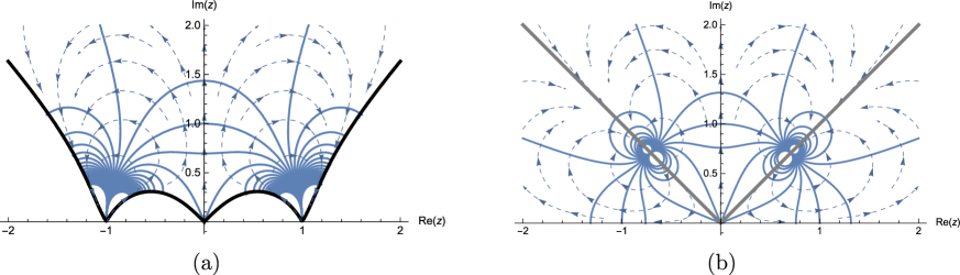
Figure 4: The equal-time contours of a string for: (a) the weighting function (3.40), which has forth-order zeros at $z=\pm 1$; and (b) the weighting function (3.45), which has zeros except at $z=\pm 1$. (Dashed lines with arrows denote evolution of time $t$. Thick lines denote branch cuts.)

As seen in Fig. 4 (a), a string propagates in a partial region of the $z$ plane, and this is a different point from the previous case in Fig. 1 (a). This behavior is clarified by the differential equation

$$\frac{dw}{dz}=\frac{1}{g(z)}.$$ (3.42)

If $g(z)$ has zeros as $g(z)\sim a_{\pm}(z\mp 1)^{n}+\cdots$, $w$ is expanded near the zeros as

$$w\sim-\frac{1}{(n-1)a_{\pm}}\,(z\mp 1)^{-n+1}+\cdots.$$ (3.43)

From this asymptotics, we find that $w$ goes around infinity if $z$ rotates by $2\pi/(n-1)$ around $z=\pm 1$. As a result, the $z$ plane is divided into $n-1$ parts due to the branch cuts. Therefore, in the second-order case ($n=2$), the region swept by a string consists of one piece of the whole $z$ plane, and in the forth-order case ($n=4$), it is a partial region of the $z$ plane. We note that the angle of the region at $z=\pm 1$ is $\pi/(n-1)$.

Secondly, let us consider the solution generated by

$$e^{h(z)}=\frac{(-1)^{l}}{4}\left(z^{l}+\frac{(-1)^{l}}{z^{l}}\right)^{2}\ \ \ (l=1,2,\dots).$$ (3.44)

The case of $l=1$ corresponding to (2.3) is discussed in the previous section as the second-order-zero case. These solutions were studied in [14, 32, 27] and vanishing physical cohomology was proved. All the numerical studies and homotopy operators indicate that these are the same tachyon vacuum solution as the case of $l=1$ [16, 17, 18]. However, these solutions have zeros at points other than $z=\pm 1$ and, particularly for the even-$l$ cases, they do not have zeros at $z=\pm 1$. So we cannot apply the SSLD mechanism in the previous section directly to these cases.

As a characteristic example, we consider the weighting function for $l=2$:

$$g(z)=\frac{z}{4}\left(z^{2}+\frac{1}{z^{2}}\right)^{2}.$$ (3.45)

This function has zeros at the fourth roots of $-1$, $z=\exp(\pm i(2k-1)\pi/4)\ \ (k=1,2)$, which are not equal to $\pm 1$. The complex coordinate for the holomorphic part is given by

$$w=\frac{-1}{1+z^{4}},$$ (3.46)

and then the unit semicircle ($t={\rm Re}\,w=-1/2$) moves as depicted in Fig. 4 (b). From this figure, we notice that the open string boundaries, which are on the real axis, move while they are static at $z=\pm 1$ in the case of $l=1$ (Fig. 1 (a)), but the zeros of (3.45) are fixed during the propagation of a string in the $z$ plane.

Before considering the $z$ plane, we recapitulate the SSLD mechanism in terms of the string picture. In SSLD, open string boundaries no longer propagate due to zeros of $g(z)$ and so the worldsheet generated by such a string becomes a closed surface without boundaries. From the viewpoint of the doubling trick, a sphere consisting of holomorphic and antiholomorphic disks is pinched along an open string boundary, and then it splits into two spheres, which correspond to holomorphic and antiholomorphic surfaces of a closed string. Operators on the holomorphic sphere are uncorrelated with those on the antiholomorphic sphere due to commuativity of the Virasoro operators, $[{\cal L}_{\kappa},\,\tilde{\cal L}_{\kappa^{\prime}}]=0$. After all, the pinch of an open string boundary means that the endpoints of an open string are bounded each other and then the open string becomes a closed string in SSLD. In other words, a closed string as a result of the doubling trick is pinched at two points corresponding to the open string endpoints and then it separates to two closed strings, as depicted in Fig. 5 (a).

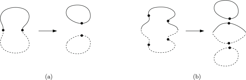
Figure 5: String pictures before and after SSLD. The solid and dashed lines correspond to holomorphic and antiholomorphic parts of a string. (a) The case of the weighting function (2.3). As a result of SSLD, open string boundaries (black dots) become joined and an open string divides to holomorphic and antiholomorphic strings. (b) The case of (3.45). The black dots represent the points of zeros of the weighting function. SSLD leads to the division of an open string into one closed and one open string.

We apply this picture of SSLD to the case of $l=2$. If we use the usual parametrization of an open string with $\sigma\ \ (0\leq\sigma\leq\pi)$, the points $\sigma=\pi/4,\ 3\pi/4$ do not propagate in this vacuum due to the zeros of $g(z)$. The open string is bounded at these points and it separates to a closed string, which corresponds to $\pi/4<\sigma<3\pi/4$, and an open string as in Fig. 5 (b). Finally, we obtain an open string in addition to a closed string at this vacuum, although we have no open strings at the tachyon vacuum.

This inconsistency is resolved by considering physical observables in open SFT. A gauge invariant observable in open SFT is given by

$$\big{<}\Psi\big{|}{\cal V}\big{>}_{\rm OSFT}\,,$$ (3.47)

where $\Psi$ is an open string field and $\big{|}{\cal V}\big{>}_{\rm OSFT}$ defined in (3.12) corresponds to an on-shell closed string vertex operator. The point is that the closed string vertex operator in $\big{|}{\cal V}\big{>}_{\rm OSFT}$ is inserted at $\sigma=\pi/2$. Therefore, at this vacuum, only the resulting closed string can be coupled with the closed string vertex operator and the separated open string has no interaction with the vertex. If we calculate perturbatively a correlation function of these observables, the resulting closed string is coupled to the external closed string vertex and so provides closed string worldsheets with the vertex. However, the separated open string gives worldsheets with no external vertex, i.2., stringy vacuum bubble diagrams. Hence, the closed string consisting of the inner part of an open string contributes to physical observables, but the open string consisting of the outer part of an open string is completely irrelevant to the closed vertex operator.

Returning to the $z$ plane of string propagation, we have branch cuts along $\arg z=\pi/4,3\pi/4$ as a result of the decomposition of an open string at this vacuum. The upper quarter plane includes the trajectory of the string midpoint $\sigma=\pi/2$. Since the branch cuts $\arg z=\pi/4$ and $\arg z=3\pi/4$ are identified, the upper quarter plane provides a holomorphic closed string surface as in the case of $l=1$. As a result of SSLD, only the correlation function on this plane contributes to observables. As far as physical observables are concerned, we conclude that the weighting function with (3.45) also provides holomorphic and antiholomorphic sectors of a closed string.

4 Concluding remarks

In this paper, we have studied SSLD in open string systems and clarified that the left and right moving modes in the SSLD system are decoupled and uncorrelated by zeros of the weighting function of the Hamiltonian. We have shown that, as a result of the decoupling, the SSLD system is equivalent to a closed string system, in the sense that we find holomorphic and antiholomorphic Virasoro algebra in the SSLD system.

Next, we considered open SFT expanded around the identity-based tachyon vacuum solution. We have found that the modified BRST operator is decomposed to holomorphic and antiholomorphic parts, which are anti-commutative and nilpotent. These operators are analogous to closed string BRST operators and so the gauge symmetry of the theory is regarded as that of closed string field theories. By using these BRST operators, we have constructed the local operators in the tachyon vacuum, including the energy-momentum tensor, ghost and anti-ghost fields, the ghost number current, and the BRST current. It is a remarkable feature that these operators depend on the frame of the worldsheet, which is chosen by the identity-based tachyon vacuum solution. From these operators, we have found the continuous Virasoro algebra and the ghost number operator. The important point is that these have holomorphic and antiholomorphic parts, which are realized by the SSLD mechanism.

The theory at the identity-based tachyon vacuum solution possesses a gauge symmetry generated by the holomorphic and antiholomorphic BRST operators, which is identified with a gauge symmetry of closed string field theories. Since gauge symmetry is an essential ingredient in SFT, we conjecture that the theory at the tachyon vacuum provides a kind of closed string field theory. That is, it is expected that the theory includes the dynamics of closed strings, although the field in the theory is an open string field. Actually, observables of pure closed strings might be calculable in terms of gauge invariants in this theory. It is known that a similar situation has occurred in matrix theories, where closed string amplitudes are obtained in terms of matrices replacing an open string field [33, 34]. More interestingly, the theory has only a cubic interaction, which is simpler than conventional covariant closed string field theories. As a first step to such a closed string field theory, it will be worth finding a method to calculate the observables of closed strings in this vacuum.

We should comment on the cohomology of the modified BRST operator at the tachyon vacuum. As proved in [14, 27], the modified BRST operator has vanishing cohomology and so the theory seems to have not only no open strings but also no closed strings at the tachyon vacuum. This apparent contradiction is immediately resolved if one considers closed strings at the perturbative vacuum. The BRST cohomology at the perturbative vacuum includes a physical open string spectrum only, but on-shell closed string states can be introduced as the state (3.12), which provides a gauge invariant observable in SFT. Therefore, at the perturbative vacuum, a correlator of the gauge invariant observables leads to a closed string amplitude [28], which is explicitly calculated in [37]. Similarly, a closed string state is included as the gauge invariant observable given by the state (3.12) even at the tachyon vacuum and so there is a possibility of deriving closed string observables in spite of the vanishing cohomology.

While closed string states are related to the state (3.12), it is important to clarify the representation of the continuous Virasoro algebra. It is known that the vacuum of the discrete SSD system is exactly equal to that of the closed system [3]. Analogously, the vacuum for the continuous Virasoro algebra is expected to correspond to that of closed string theories, although the correspondence is still unclear. Furthermore, it is much more difficult to understand excited states for the continuous Virasoro algebra. It will be interesting in future work to investigate representations of the continuous Virasoro algebra, if possible, by referring to SFT. In an appropriate representation space, the cohomology of the modified BRST operator might be nontrivial and related to closed string states.

Finally, we should comment on the level-matching condition, which is imposed on a conventional closed string field to assure the $\sigma$ translational invariance of a closed string. In conventional closed SFTs, it is imposed on a closed string field as $(L_{0}-\tilde{L}_{0})\Phi=0$. However, it is difficult to find such a condition in open SFT on the identity-based tachyon vacuum. For instance, it is easily found that the open string field or the closed string state do not satisfy a straightforward extension of the level-matching condition: $({\cal L}_{0}-\tilde{\cal L}_{0})\Psi=0$ or $({\cal L}_{0}-\tilde{\cal L}_{0})\left|\cal V\right>_{\rm OSFT}=0$. This is not a problem because the open string field and the closed string state do not have uniformity due to the fixed boundary points or the midpoint of a string. This suggests that the level-matching condition is not necessarily required in closed string field theories and our theory indicates the possibility of a closed SFT without the condition. On the other hand, this possibility is pursued in SFT in terms of a conventional closed string field [35]. It will be interesting to understand the relation between these SFTs.

Appendix A Commutation relations for the SSLD Hamiltonian

For the energy-momentum tensor on the $z$ plane, $T(z)=\sum_{n\in\mathbb{Z}}L_{n}z^{-n-2}$, satisfying the OPE

$$T(z)T(z^{\prime})\sim\frac{c/2}{(z-z^{\prime})^{4}}+\frac{2}{(z-z^{\prime})^{2}}T(z^{\prime})+\frac{1}{z-z^{\prime}}\partial T(z^{\prime}),$$ (A.1)

we have the Virasoro algebra with the central charge $c$ :

$$[L_{m},L_{n}]=(m-n)L_{m+n}+\frac{c}{12}(m^{3}-m)\delta_{m+n,0}.$$ (A.2)

With this algebra, we can derive (2.5) as

$$[T(z),T(z^{\prime})] =\sum_{m,n\in\mathbb{Z}}z^{-m-2}z^{\prime-n-2}\left((m-n)L_{m+n}+\frac{c}{12}(m^{3}-m)\delta_{m+n,0}\right)$$

$$=\sum_{m,l\in\mathbb{Z}}(m+1)z^{-m-2}z^{\prime m-l-2}L_{l}-\sum_{n,l\in\mathbb{Z}}(n+1)z^{n-l-2}z^{\prime-n-2}L_{l}-\frac{c}{12}\partial^{3}\sum_{m\in\mathbb{Z}}z^{-m+1}z^{\prime m-2}$$

$$=-\partial\sum_{m\in\mathbb{Z}}z^{-m-1}z^{\prime m}T(z^{\prime})+\partial^{\prime}\sum_{n\in\mathbb{Z}}z^{n}z^{\prime-n-1}T(z)-\frac{c}{12}\partial^{3}\sum_{m\in\mathbb{Z}}z^{-m+1}z^{\prime m-2}$$

$$=-\partial\delta(z,z^{\prime})T(z^{\prime})+\partial^{\prime}\delta(z,z^{\prime})T(z)-\frac{c}{12}\partial^{3}\delta(z,z^{\prime})$$

$$=-(T(z)+T(z^{\prime}))\partial\delta(z,z^{\prime})-\frac{c}{12}\partial^{3}\delta(z,z^{\prime}),$$ (A.3)

($\partial=\frac{\partial}{\partial z},~{}\partial^{\prime}=\frac{\partial}{\partial z^{\prime}}$), where we have used the notion that the delta function on the unit circle, $\delta(z,z^{\prime})=\sum_{n\in\mathbb{Z}}z^{-n-1}z^{\prime n}$, satisfies

$$\partial\delta(z,z^{\prime}) =-\partial^{\prime}\delta(z,z^{\prime}).$$ (A.4)

Actually, the commutation relation (2.5) holds for any frame. For a conformal transformation $w=w(z)$, the energy-momentum tensor $T(w)$ is given by $T(w)=(\frac{dz}{dw})^{2}\left(T(z)-\frac{c}{12}\{w,z\}\right)$, where $\{w(z),\,z\}=\frac{w^{\prime\prime\prime}}{w^{\prime}}-\frac{3}{2}(\frac{w^{\prime\prime}}{w^{\prime}})^{2}$ is the Schwarzian derivative, and the commutation relation is computed with (2.5) as follows:

$$[T(w),T(w^{\prime})] =\left(\frac{dz}{dw}\right)^{2}\left(\frac{dz^{\prime}}{dw^{\prime}}\right)^{2}\left(-(T(z)+T(z^{\prime}))\partial\delta(z,z^{\prime})-\frac{c}{12}\partial^{3}\delta(z,z^{\prime})\right)$$

$$=-\left[T(w)\left(\frac{dz^{\prime}}{dw^{\prime}}\right)^{2}+T(w^{\prime})\left(\frac{dz}{dw}\right)^{2}\right]\partial\delta(z,z^{\prime})$$

$$\quad\,-\frac{c}{12}\left(\frac{dz}{dw}\right)^{2}\left(\frac{dz^{\prime}}{dw^{\prime}}\right)^{2}\left[\partial^{3}\delta(z,\,z^{\prime})+\left(\{w,\,z\}+\{w^{\prime},\,z^{\prime}\}\right)\partial\delta(z,\,z^{\prime})\right].$$ (A.5)

Here, for the transformation $w=w(z)$, we define the delta function as

$$\delta(w,\,w^{\prime})=\frac{dz}{dw}\delta(z,\,z^{\prime})=\frac{dz^{\prime}}{dw^{\prime}}\delta(z,\,z^{\prime}).$$ (A.6)

The integration range is changed to a contour $C$ for $w$, which is the image of the unit circle on the $z$ plane. Corresponding to (2.6), its normalization is given by

$$\int_{C}\frac{dw}{2\pi i}\delta(w,\,w^{\prime})=1.$$ (A.7)

For the delta function, we find the following relations:

$$\partial_{w}\delta(w,\,w^{\prime})=\frac{dz}{dw}\frac{dz^{\prime}}{dw^{\prime}}\partial\delta(z,\,z^{\prime})=\left(\frac{dz}{dw}\right)^{2}\partial\delta(z,z^{\prime})+\frac{d^{2}z}{dw^{2}}\delta(z,z^{\prime})=-\partial_{w}^{\prime}\delta(w,w^{\prime}),$$ (A.8)

$$\partial_{w}^{3}\delta(w,\,w^{\prime})=\left(\frac{dz}{dw}\right)^{2}\left(\frac{dz^{\prime}}{dw^{\prime}}\right)^{2}\left[\partial^{3}\delta(z,\,z^{\prime})+\left(\{w,\,z\}+\{w^{\prime},\,z^{\prime}\}\right)\partial\delta(z,\,z^{\prime})\right],$$ (A.9)

where $\partial_{w}=\frac{\partial}{\partial w},~{}\partial_{w}^{\prime}=\frac{\partial}{\partial w^{\prime}}$. By using (A.8) and (A.9), (A.5) can be rewritten as:

$$[T(w),\,T(w^{\prime})]=-(\,T(w)+T(w^{\prime})\,)\,\partial_{w}\delta(w,w^{\prime})-\frac{c}{12}\partial_{w}^{3}\delta(w,w^{\prime}),$$ (A.10)

which is the same form as (2.5).

For the left and right moving modes of the Hamiltonian, $H^{\pm}_{g}$ (2.2), the commutation relation (2.5) is applied as

$$[H^{+}_{g},H^{-}_{g}] =\int_{C_{+}}\frac{dz}{2\pi i}\int_{C_{-}}\frac{dz^{\prime}}{2\pi i}g(z)g(z^{\prime})\left(-(T(z)+T(z^{\prime}))\partial\delta(z,z^{\prime})-\frac{c}{12}\partial^{3}\delta(z,z^{\prime})\right)$$

$$=\int_{C_{+}}\frac{dz}{2\pi i}\int_{C_{-}}\frac{dz^{\prime}}{2\pi i}\left(g(z^{\prime})\left(\partial g(z)(T(z)+T(z^{\prime}))+g(z)\partial T(z)\right)-\frac{c}{12}\partial^{2}g(z)\partial g(z^{\prime})\right)\delta(z,z^{\prime})$$

$$=0,$$ (A.11)

where we have used the condition $g(\pm 1)=\partial g(\pm 1)=0$, eq. (A.4) and

$$\int_{C_{+}}\frac{dz}{2\pi i}\int_{C_{-}}\frac{dz^{\prime}}{2\pi i}f_{1}(z)f_{2}(z^{\prime})\delta(z,z^{\prime})=0,$$ (A.12)

which is obtained in the same way as that in [13] for the left/right half of the unit circle.

Appendix B Integration along $C_{\pm 1}^{s_{\rm max}}$

We illustrate the evaluation of the integral along $C_{\pm 1}^{s_{\rm max}}$:

$$\int_{C_{\pm 1}^{s_{\rm max}}}\frac{dz}{2\pi i}g(z)f_{\kappa}(z)T(z).$$ (B.1)

Following the definition of $C_{\pm 1}^{s_{\rm max}}$ in §2.3, we change the integration variable to the time $t$:

eq. (B.1) $$= \int_{t\mp\varDelta t}^{t\pm\varDelta t}\frac{dt}{2\pi i}g(z)^{2}e^{\kappa(t\mp is_{\rm max})}T(z),$$ (B.2)

where we have used $dz/dt=g(z)$ and $f_{\kappa}(z)=\exp(\kappa(t+is))$.

Suppose that the operator $T(z)$ is bounded from above in correlation functions, i.e., $\big{|}\,\big{<}T(z)\cdots\big{>}\,\big{|}\leq M\big{|}\,\big{<}\cdots\big{>}\,\big{|}$. Substituting (2.3) for the above, we find

$$\left|\,\mbox{eq.~{}(\ref{eq:C+1smax})}\,\right| \leq \int_{t-\varDelta t}^{t+\varDelta}\frac{dt}{2\pi}\frac{e^{\kappa t}M}{\sqrt{(t^{2}+s_{\rm max}^{2})^{3}\{(t+2)^{2}+s_{\rm max}^{2}\}}}.$$ (B.3)

Here we have used

$$g(z)^{2}=\frac{1}{(t+is)^{3}(t+2+is)},$$ (B.4)

which is derived from $t+is=2/(z^{2}-1)$ and (2.3). From the mean value theorem, there exists $\xi$ in $(t-\varDelta t,\,t+\varDelta t)$ such that

RHS of (B.3) $$= 2\varDelta t\,\frac{1}{2\pi}\frac{Me^{\kappa\xi}}{\sqrt{(\xi^{2}+s_{\rm max}^{2})^{3}\{(\xi+2)^{2}+s_{\rm max}^{2}\}}}.$$ (B.5)

By taking the limit $s_{\rm max}\rightarrow\infty$, the above approaches zero for a fixed value of $\varDelta t$. Therefore, we obtain

$$\lim_{s_{\rm max}\rightarrow\infty}\int_{C_{\pm 1}^{s_{\rm max}}}\frac{dz}{2\pi i}g(z)f_{\kappa}(z)T(z)=0.$$ (B.6)

As a result, we can add the integral along ${C_{\pm 1}^{s_{\rm max}}}$ to (2.23).

Here, we show that the essential singularity of $f_{\kappa}(z)$ has no effect on the integration of the commutator of the Virasoro algebra. The important point is that we quantize the system by the Hamiltonian ${\cal L}_{0}+\tilde{\cal L}_{0}$. So, for any weighting function $g(z)$, $f_{\kappa}(z)$ is given by the differential equation (2.19) and it is written as

$$f_{\kappa}(z)=e^{\kappa(t+is)}.$$ (B.7)

On the $z$ plane, as a result of the quantization, each contour of string propagation starts from and ends at the fixed points along the same direction. In the above example, it approaches $z=\pm 1$ parallel to the imaginary axis. In general, a function takes the value of any complex number in the neighborhood of its essential singularity. However, due to the direction of the contours, $f_{\kappa}(z)$ does not diverge if $z$ approaches the fixed point as $s_{\rm max}$ goes to infinity in the integration. Hence, in general, the essential singularity in $f_{\kappa}(z)$ becomes manageable by the quantization procedure of SSLD.

Appendix C Anti-commutation relations for the modified BRST operator

Expanding the BRST current $j_{\rm B}(z)=cT_{\rm mat}(z)+bc\partial c(z)+\frac{3}{2}\partial^{2}c(z)$ and the ghost $c(z)$ as

$$j_{{\rm B}}(z)=\sum_{n=-\infty}^{\infty}Q_{n}z^{-n-1},\qquad c(z)=\sum_{n=-\infty}^{\infty}c_{n}z^{-n+1},$$ (C.1)

we have relations among the modes:

$$\{Q_{m},Q_{n}\} =2mn\{Q_{\rm B},c_{m+n}\}, \{Q_{m},c_{n}\} =\{Q_{\rm B},c_{m+n}\},$$ (C.2)

($Q_{\rm B}=Q_{0}$) and then the relations

$$\{j_{\rm B}(z),j_{\rm B}(z^{\prime})\} =2\partial\partial^{\prime}\left(\delta(z,z^{\prime})\{Q_{\rm B},c(z^{\prime})\}\right), \{j_{\rm B}(z),c(z^{\prime})\} =\delta(z,z^{\prime})\{Q_{\rm B},c(z^{\prime})\}$$ (C.3)

are obtained in a similar way to the derivation in (A.3). From these, (3.8), (3.9) and (3.10) are demonstrated using (A.12) and

$$\int_{C_{\pm}}\frac{dz}{2\pi i}\int_{C_{\pm}}\frac{dz^{\prime}}{2\pi i}f_{1}(z)f_{2}(z^{\prime})\delta(z,z^{\prime})=\int_{C_{\pm}}\frac{dz}{2\pi i}f_{1}(z)f_{2}(z),$$ (C.4)

which is derived similarly to (A.12). In particular, the conditions $f(\pm 1)=g(\pm 1)=0$ are used for $\{Q_{\pm}(f),Q_{\pm}(g)\}$ and $\{Q_{\pm}(f),Q_{\mp}(g)\}$. For the operators $Q^{\prime}_{\pm}$ (3.5), we can compute them as

$$\{Q_{\pm}^{\prime},Q_{\pm}^{\prime}\} =\{Q_{\pm}(e^{h}),Q_{\pm}(e^{h})\}-2\{Q_{\pm}(e^{h}),C_{\pm}((\partial h)^{2}e^{h})\}$$

$$=2\{Q_{\rm B},C_{\pm}(\partial e^{h})^{2}\}-2\{Q_{\rm B},C_{\pm}((\partial h)^{2}e^{2h}\}=0$$ (C.5)

with (3.8) and (3.9) because $e^{h(z)}$ vanishes at $z=\pm 1$ by assumption. Similarly, from (3.10), we have

$$\{Q_{\pm}^{\prime},Q_{\mp}^{\prime}\} =\{Q_{\pm}(e^{h}),Q_{\mp}(e^{h})\}-\{Q_{\pm}(e^{h}),C_{\mp}((\partial h)^{2}e^{h})\}-\{Q_{\mp}(e^{h}),C_{\pm}((\partial h)^{2}e^{h})\}=0.$$ (C.6)

Therefore, the nilpotency of $Q_{\pm}^{\prime}$ and anti-commutativity (3.11) are proved.

Appendix D $Q^{\prime}_{\pm}$ invariance of $|\mathcal{V}\rangle_{\rm OSFT}$

Here, we show (3.13), namely, $Q^{\prime}_{\pm}$ invariance of $|\mathcal{V}\rangle_{\rm OSFT}$ (3.12). $Q_{\pm}^{\prime}$ (3.5) can be expressed as

$$Q_{\pm}^{\prime} =\int_{C_{\pm}}\frac{dz}{2\pi i}F(z)j_{{\rm B}}(z)+\int_{C_{\pm}}\frac{dz}{2\pi i}G(z)c(z),$$ (D.1)

$$F(z)=e^{h(z)},\qquad G(z)=-(\partial h(z))^{2}e^{h(z)}.$$ (D.2)

From the relation $h(-1/z)=h(z)$, we have

$$F(-1/z)=F(z),\qquad G(-1/z)=z^{4}G(z)$$ (D.3)

and therefore we can expand the weighting functions $F(z)$ and $G(z)$ as

$$F(z)=\sum_{n=0}^{\infty}a_{n}(z^{n}+(-1)^{n}z^{-n}),\qquad G(z)=z^{-2}\sum_{n=0}^{\infty}a_{n}^{\prime}(z^{n}+(-1)^{n}z^{-n})$$ (D.4)

on the unit circle $|z|=1$, where $a_{n}$ and $a_{n}^{\prime}$ are constants. Using the above and the mode expansions of the BRST current and ghost (C.1), (D.1) can be rewritten as

$$Q_{\pm}^{\prime} =a_{0}Q_{0}+\sum_{n=1}^{\infty}\frac{a_{n}}{2}(Q_{n}+(-1)^{n}Q_{-n})+a_{0}^{\prime}c_{0}+\sum_{n=1}^{\infty}\frac{a_{n}^{\prime}}{2}(c_{n}+(-1)^{n}c_{-n})$$

$$\quad\mp\frac{i}{\pi}\Biggl{[}\sum_{k=0}^{\infty}\frac{2a_{0}}{2k+1}(Q_{2k+1}-Q_{-2k-1})+\sum_{k=0}^{\infty}\frac{2a_{0}^{\prime}}{2k+1}(c_{2k+1}-c_{-2k-1})$$

$$\qquad\qquad+\sum_{n=1}^{\infty}\sum_{k=0}^{\infty}\frac{a_{n}}{2k+1}(Q_{n+2k+1}-(-1)^{n}Q_{-n-2k-1}-(Q_{n-2k-1}-(-1)^{n}Q_{-n+2k+1}))$$

$$\qquad\qquad+\sum_{n=1}^{\infty}\sum_{k=0}^{\infty}\frac{a_{n}^{\prime}}{2k+1}(c_{n+2k+1}-(-1)^{n}c_{-n-2k-1}-(c_{n-2k-1}-(-1)^{n}c_{-n+2k+1}))\Biggr{]},$$ (D.5)

where use has been made of

$$\int_{C_{\pm}}\frac{dz}{2\pi i}z^{-1-n} =\begin{cases}\frac{1}{2}&(n=0)\\ 0&(n=2k\,,\ k\in\mathbb{Z}\setminus\!\{0\})\\ \frac{\mp i}{n\pi}&(n=2k+1\,,\ k\in\mathbb{Z}).\end{cases}$$ (D.6)

In particular, we find that $Q^{\prime}_{\pm}$ is given by a linear combination of

$$Q_{n}+(-1)^{n}Q_{-n}\,,\qquad c_{n}+(-1)^{n}c_{-n}\,,\qquad(n\in\mathbb{Z}),$$ (D.7)

and hence we have (3.13), thanks to

$$\left(Q_{n}+(-1)^{n}Q_{-n}\right)|\mathcal{V}\rangle_{\rm OSFT}=0,\qquad\left(c_{n}+(-1)^{n}c_{-n}\right)|\mathcal{V}\rangle_{\rm OSFT}=0,$$ (D.8)

which can be shown as in [36] using a method in [38].

Appendix E Commutation relations for the deformed Hamiltonian at the tachyon vacuum

For the holomorphic and antiholomorphic parts of the Hamiltonian, $H_{\pm}$ (3.19), commutation relations involving the ghost number current $j_{\rm gh}(z)=cb(z)=\sum_{n\in\mathbb{Z}}q_{n}z^{-n-1}$ are necessary. From the OPEs, we have

$$[L_{m},q_{n}] =-nq_{m+n}-\frac{3}{2}m(m+1)\delta_{m+n,0}, [q_{m},q_{n}] =m\delta_{m+n,0},$$ (E.1)

and then

$$[T(z),j_{\rm gh}(z^{\prime})] =\partial^{\prime}\delta(z,z^{\prime})j_{\rm gh}(z)-\frac{3}{2}\partial^{2}\delta(z,z^{\prime}), [j_{\rm gh}(z),j_{\rm gh}(z^{\prime})] =-\partial\delta(z,z^{\prime}),$$ (E.2)

are derived in a similar way to (A.3). Using (2.5), (E.2) and (A.12), we have

$$[H_{+},H_{-}]$$

$$=\int_{C_{+}}\frac{dz}{2\pi i}\int_{C_{-}}\frac{dz^{\prime}}{2\pi i}zz^{\prime}[e^{h}T(z)+\partial e^{h}j_{\rm gh}(z),e^{h}T(z^{\prime})+\partial e^{h}j_{\rm gh}(z^{\prime})]$$

$$=\int_{C_{+}}\frac{dz}{2\pi i}\int_{C_{-}}\frac{dz^{\prime}}{2\pi i}zz^{\prime}\biggl{(}-e^{h(z)}e^{h(z^{\prime})}\left((T(z)+T(z^{\prime}))\partial\delta(z,z^{\prime})+\frac{c}{12}\partial^{3}\delta(z,z^{\prime})\right)-\partial e^{h(z)}\partial e^{h(z^{\prime})}\partial\delta(z,z^{\prime})$$

$$\qquad+e^{h(z)}\partial e^{h(z^{\prime})}\left(\partial^{\prime}\delta(z,z^{\prime})j_{\rm gh}(z)-\frac{3}{2}\partial^{2}\delta(z,z^{\prime})\right)-\partial e^{h(z)}e^{h(z^{\prime})}\left(\partial\delta(z,z^{\prime})j_{\rm gh}(z^{\prime})-\frac{3}{2}\partial^{\prime 2}\delta(z,z^{\prime})\right)\biggr{)}$$

$$=\int_{C_{+}}\frac{dz}{2\pi i}\int_{C_{-}}\frac{dz^{\prime}}{2\pi i}\biggl{(}\partial(ze^{h})z^{\prime}e^{h(z^{\prime})}(T(z)+T(z^{\prime}))-\frac{c}{12}\partial^{2}(ze^{h})\partial^{\prime}(z^{\prime}e^{h})+\partial(z\partial e^{h})z^{\prime}\partial^{\prime}e^{h}$$

$$\qquad-ze^{h}j_{\rm gh}(z)\partial^{\prime}(z^{\prime}\partial^{\prime}e^{h})-\frac{3}{2}\partial^{2}(ze^{h})z^{\prime}\partial^{\prime}e^{h}+\partial(z\partial e^{h})z^{\prime}e^{h}j_{\rm gh}(z^{\prime})+\frac{3}{2}z\partial e^{h}\partial^{\prime 2}(z^{\prime}e^{h})\biggr{)}\delta(z,z^{\prime})$$

$$=0,$$ (E.3)

because $e^{h(z)}$ has second-order zeros at $z=\pm 1$ by assumption. Actually, the central charge for $T(z)$ is zero in the context of (3.19).

Appendix F BRST operators, Virasoro operators and ghost number at the tachyon vacuum

The BRST current $j_{\rm B}(z)$ and the ghost $c(z)$ are primary fields with conformal weights $1$ and $-1$, respectively, and hence we have

$$[Q_{m},L_{n}] =mQ_{m+n}, [c_{m},L_{n}] =(2n+m)c_{m+n}$$ (F.1)

which imply the commutation relations

$$[j_{\rm B}(z),T(z^{\prime})] =-\partial\delta(z,z^{\prime})j_{\rm B}(z^{\prime}), [c(z),T(z^{\prime})] =\partial\delta(z,z^{\prime})c(z)-2\delta(z,z^{\prime})\partial c(z^{\prime}).$$ (F.2)

For the ghost number current $j_{\rm gh}(z)$, the modes satisfy the commutation relations

$$[Q_{m},q_{n}] =-Q_{m+n}+2mnc_{m+n}, [c_{m},q_{n}] =-c_{m+n},$$ (F.3)

and they give

$$[j_{\rm B}(z),j_{\rm gh}(z^{\prime})] =-\delta(z,z^{\prime})j_{\rm B}(z^{\prime})+2\partial\partial^{\prime}\left(\delta(z,z^{\prime})c(z^{\prime})\right), [c(z),j_{\rm gh}(z^{\prime})] =-\delta(z,z^{\prime})c(z^{\prime}).$$ (F.4)

If we define $j^{\prime}_{\rm B}(z)$ such as $Q^{\prime}_{\pm}=\int_{C_{\pm}}\frac{dz}{2\pi i}j^{\prime}_{\rm B}(z)$ by

$$j^{\prime}_{\rm B}(z) =e^{h(z)}j_{\rm B}(z)-(\partial h(z))^{2}e^{h(z)}c(z),$$ (F.5)

we can compute a commutation relation with ${\mathcal{T}}(z)$ (3.20) using (F.2) and (F.4) as

$$[j^{\prime}_{\rm B}(z),{\mathcal{T}}(z^{\prime})] =-\partial\left(e^{h(z)}\delta(z,z^{\prime})j_{\rm B}(z^{\prime})\right)$$

$$\quad+\partial\left(2e^{h(z)}\partial h(z^{\prime})\partial^{\prime}(\delta(z,z^{\prime})c(z^{\prime}))+e^{-h(z^{\prime})}(\partial e^{h(z^{\prime})})^{2}\delta(z,z^{\prime})c(z^{\prime})\right).$$ (F.6)

Integrating the above, we have

$$[Q^{\prime}_{\pm},g(z^{\prime})f_{\kappa}(z^{\prime}){\mathcal{T}}(z^{\prime})] =\mp\left[z^{\prime}e^{h(z)}e^{h(z^{\prime})}e^{\kappa w^{\prime}}\delta(z,z^{\prime})j_{\rm B}(z^{\prime})\right]^{z=-1}_{z=1}$$

$$\quad\pm\left[2z^{\prime}e^{h(z)}\partial e^{h(z^{\prime})}e^{\kappa w^{\prime}}\partial^{\prime}(\delta(z,z^{\prime})c(z^{\prime}))+z^{\prime}(\partial e^{h(z^{\prime})})^{2}e^{\kappa w^{\prime}}\delta(z,z^{\prime})c(z^{\prime})\right]^{z=-1}_{z=1}$$ (F.7)

for $g(z^{\prime})=z^{\prime}e^{h(z^{\prime})}$ and $f_{\kappa}(z^{\prime})=e^{\kappa w^{\prime}}$ with $w^{\prime}=\int^{z^{\prime}}\frac{dz}{g(z)}$. Noting that $e^{h(z)}$ has second-order zeros at $z=\pm 1$ by assumption and assuming that $|e^{\kappa w^{\prime}}|$ is bounded from above near $z^{\prime}=\pm 1$ along the unit circle, we obtain (3.23) by integrating (F.7) along $C_{\pm}$.

From (F.4), we have a commutation relation:

$$[j_{\rm B}^{\prime}(z),j_{\rm gh}(z^{\prime})] =-\delta(z,z^{\prime})j^{\prime}_{\rm B}(z^{\prime})+\partial^{\prime}\left(2e^{h(z)}\partial\delta(z,z^{\prime})c(z^{\prime})\right).$$ (F.8)

Integrating the above and using (C.4), we have

$$\int_{C_{\pm}}\frac{dz}{2\pi i}\int_{C_{\pm}}\frac{dz^{\prime}}{2\pi i}[j_{\rm B}^{\prime}(z),j_{\rm gh}(z^{\prime})] =-\int_{C_{\pm}}\frac{dz}{2\pi i}j^{\prime}_{\rm B}(z)\mp\left[\int_{C_{\pm}}\frac{dz}{2\pi i}2(\partial e^{h(z)})\delta(z,z^{\prime})c(z^{\prime})\right]^{z^{\prime}=-1}_{z^{\prime}=1}.$$ (F.9)

Because $\partial e^{h(z)}$ vanishes at $z=\pm 1$, the second term on the right-hand side is zero. Similarly, from (A.12), we have

$$\int_{C_{\pm}}\frac{dz}{2\pi i}\int_{C_{\mp}}\frac{dz^{\prime}}{2\pi i}[j_{\rm B}^{\prime}(z),j_{\rm gh}(z^{\prime})] =0.$$ (F.10)

These relations imply (3.32).

On the modified BRST current, we note that the difference of (3.38) and (F.5) is computed as

$${\mathcal{J}}_{\rm B}(z)-j^{\prime}_{\rm B}(z) =\partial\left(2(\partial e^{h(z)})c(z)\right)$$ (F.11)

and therefore (3.39) holds.

It is possible to provide an alternative derivation of (3.23). First, we introduce continuous modes for the anti-ghost field at the tachyon vacuum:

$$b_{\kappa}^{\prime}=\int_{C_{+}}\frac{dz}{2\pi i}g(z)f_{\kappa}(z)b^{\prime}(z),~{}~{}~{}~{}\tilde{b}_{\kappa}^{\prime}=\int_{C_{-}}\frac{dz}{2\pi i}g(z)f_{\kappa}(z)b^{\prime}(z).$$ (F.12)

Since ${\cal J}_{\rm B}(z)$, $b^{\prime}(z)$, ${\cal T}(z)$ and ${\mathcal{J}}_{\rm gh}(z)$ satisfy the same OPE as the conventional ones, we find the anti-commutation relation

$$\{{\mathcal{J}}_{\rm B}(z),b^{\prime}(z^{\prime})\} =\delta(z,z^{\prime}){\mathcal{T}}(z^{\prime})-\partial\delta(z,z^{\prime}){\mathcal{J}}_{\rm gh}(z^{\prime})+\frac{3}{2}\partial^{2}\delta(z,z^{\prime}).$$ (F.13)

Integrating the above, we have

$$\{Q^{\prime}_{\pm},b_{\kappa}^{\prime}\} =\int_{C_{\pm}}\frac{dz}{2\pi i}\int_{C_{+}}\frac{dz^{\prime}}{2\pi i}g(z^{\prime})f_{\kappa}(z^{\prime}){\mathcal{T}}(z^{\prime})\delta(z,z^{\prime})$$

$$\qquad\mp\left[\int_{C_{+}}\frac{dz^{\prime}}{2\pi i}\left(g(z^{\prime})f_{\kappa}(z^{\prime}){\mathcal{J}}_{\rm gh}(z^{\prime})+\frac{3}{2}(\partial g(z^{\prime})+\kappa)f_{\kappa}(z^{\prime})\right)\delta(z,z^{\prime})\right]^{z=-1}_{z=1},$$ (F.14)

where we have assumed that $|f_{\kappa}(z^{\prime})|$ is bounded from above near $z^{\prime}=\pm 1$ along the unit circle. The second line on the right-hand side of (F.14) does not contribute by taking the same regularization as (2.22) in (F.12) and then we obtain

$$\{Q^{\prime}_{+},\,b_{\kappa}^{\prime}\} ={\mathcal{L}}_{\kappa}, \{Q^{\prime}_{-},\,b_{\kappa}^{\prime}\} =0$$ (F.15)

from (C.4), (A.12) and (3.22). Similarly,

$$\{Q^{\prime}_{-},\,{\tilde{b}}_{\kappa}^{\prime}\} ={\tilde{\mathcal{L}}}_{\kappa}, \{Q^{\prime}_{+},\,{\tilde{b}}_{\kappa}^{\prime}\} =0$$ (F.16)

are obtained. With the above anti-commutation relations, (3.11) and the Jacobi identity, eq. (3.23) is derived.

References

• [1] A. Gendiar, R. Krcmar and T. Nishino, “Spherical Deformation for One-Dimensional Quantum Systems,” Prog. Theor. Phys. 122, 953 (2009) doi:10.1143/PTP.122.953; Errata ibid 123, 393 (2010) [arXiv:0810.0622 [cond-mat.str-el]].
• [2] T. Hikihara and T. Nishino, “Connecting distant ends of one-dimensional critical systems by a sine-square deformation,” Phys. Rev. B83, 060414(R) (2011) doi:10.1103/PhysRevB.83.060414 [arXiv:1012.0472 [cond-mat.stat-mech]].
• [3] H. Katsura, “Exact ground state of the sine-square deformed XY spin chain,” J. Phys. A: Math. Theor. 44 (2011) 252001 doi:10.1088/1751-8113/44/25/252001 [arXiv:1104.1721 [cond-mat.stat-mech]].
• [4] N. Shibata and C. Hotta, “Boundary effects in the density-matrix renormalization group calculation,” Phys. Rev. B84, 115116 (2011) doi:10.1103/PhysRevB.84.115116 [arXiv:1106.6202 [cond-mat.str-el]].
• [5] I. Maruyama, H. Katsura and T. Hikihara, “Sine-square deformation of free fermion systems in one and higher dimensions,” Phys. Rev. B84, 165132 (2011) doi:10.1103/PhysRevB.84.165132 [arXiv:1108.2937 [cond-mat.stat-mech]].
• [6] H. Katsura, “Sine-square deformation of solvable spin chains and conformal field theories,” J. Phys. A 45, 115003 (2012) doi:10.1088/1751-8113/45/11/115003 [arXiv:1110.2459 [cond-mat.stat-mech]].
• [7] T. Tada, “Sine Square Deformation and String Theory,” JPS Conf. Proc.  1, 013003 (2014). doi:10.7566/JPSCP.1.013003
• [8] T. Tada, “Sine-Square Deformation and its Relevance to String Theory,” Mod. Phys. Lett. A 30, no. 19, 1550092 (2015) doi:10.1142/S0217732315500923 [arXiv:1404.6343 [hep-th]].
• [9] N. Ishibashi and T. Tada, “Infinite circumference limit of conformal field theory,” J. Phys. A 48, no. 31, 315402 (2015) doi:10.1088/1751-8113/48/31/315402 [arXiv:1504.00138 [hep-th]].
• [10] N. Ishibashi and T. Tada, “Dipolar quantization and the infinite circumference limit of two-dimensional conformal field theories,” Int. J. Mod. Phys. A 31, no. 32, 1650170 (2016) doi:10.1142/S0217751X16501700 [arXiv:1602.01190 [hep-th]].
• [11] K. Okunishi, “Sine-square deformation and Möbius quantization of 2D conformal field theory,” PTEP 2016, no. 6, 063A02 (2016) doi:10.1093/ptep/ptw060 [arXiv:1603.09543 [hep-th]].
• [12] X. Wen, S. Ryu and A. W. W. Ludwig, “Evolution operators in conformal field theories and conformal mappings: Entanglement Hamiltonian, the sine-square deformation, and others,” Phys. Rev. B 93, no. 23, 235119 (2016) doi:10.1103/PhysRevB.93.235119 [arXiv:1604.01085 [cond-mat.str-el]].
• [13] T. Takahashi and S. Tanimoto, “Marginal and scalar solutions in cubic open string field theory,” JHEP 0203, 033 (2002) doi:10.1088/1126-6708/2002/03/033 [hep-th/0202133].
• [14] I. Kishimoto and T. Takahashi, “Open string field theory around universal solutions,” Prog. Theor. Phys.  108, 591 (2002) doi:10.1143/PTP.108.591 [hep-th/0205275].
• [15] T. Takahashi and S. Zeze, “Gauge fixing and scattering amplitudes in string field theory around universal solutions,” Prog. Theor. Phys.  110, 159 (2003) doi:10.1143/PTP.110.159 [hep-th/0304261].
• [16] T. Takahashi, “Tachyon condensation and universal solutions in string field theory,” Nucl. Phys. B 670, 161 (2003) doi:10.1016/j.nuclphysb.2003.08.007 [hep-th/0302182].
• [17] I. Kishimoto and T. Takahashi, “Vacuum structure around identity based solutions,” Prog. Theor. Phys.  122, 385 (2009) doi:10.1143/PTP.122.385 [arXiv:0904.1095 [hep-th]].
• [18] I. Kishimoto, “On numerical solutions in open string field theory,” Prog. Theor. Phys. Suppl.  188, 155 (2011). doi:10.1143/PTPS.188.155
• [19] I. Kishimoto, T. Masuda and T. Takahashi, “Observables for identity-based tachyon vacuum solutions,” PTEP 2014, no. 10, 103B02 (2014) doi:10.1093/ptep/ptu136 [arXiv:1408.6318 [hep-th]].
• [20] N. Ishibashi, “Comments on Takahashi-Tanimoto’s scalar solution,” JHEP 1502, 168 (2015) doi:10.1007/JHEP02(2015)168 [arXiv:1408.6319 [hep-th]].
• [21] S. Zeze, “Gauge invariant observables from Takahashi-Tanimoto scalar solutions in open string field theory,” arXiv:1408.1804 [hep-th].
• [22] M. Schnabl, “Analytic solution for tachyon condensation in open string field theory,” Adv. Theor. Math. Phys.  10, no. 4, 433 (2006) doi:10.4310/ATMP.2006.v10.n4.a1 [hep-th/0511286].
• [23] T. Erler and M. Schnabl, “A Simple Analytic Solution for Tachyon Condensation,” JHEP 0910, 066 (2009) doi:10.1088/1126-6708/2009/10/066 [arXiv:0906.0979 [hep-th]].
• [24] N. Drukker, “On different actions for the vacuum of bosonic string field theory,” JHEP 0308, 017 (2003) doi:10.1088/1126-6708/2003/08/017 [hep-th/0301079].
• [25] N. Drukker, “Closed string amplitudes from gauge fixed string field theory,” Phys. Rev. D 67, 126004 (2003) doi:10.1103/PhysRevD.67.126004 [hep-th/0207266].
• [26] T. Takahashi, “A vacuum loop of an open string around an identity-based solution,” Prog. Theor. Phys. Suppl.  188, 163 (2011). doi:10.1143/PTPS.188.163
• [27] S. Inatomi, I. Kishimoto and T. Takahashi, “Homotopy Operators and One-Loop Vacuum Energy at the Tachyon Vacuum,” Prog. Theor. Phys.  126, 1077 (2011) doi:10.1143/PTP.126.1077 [arXiv:1106.5314 [hep-th]].
• [28] B. Zwiebach, “Interpolating string field theories,” Mod. Phys. Lett. A 7, 1079 (1992) doi:10.1142/S0217732392000951 [hep-th/9202015].
• [29] A. Hashimoto and N. Itzhaki, “Observables of string field theory,” JHEP 0201, 028 (2002) doi:10.1088/1126-6708/2002/01/028 [hep-th/0111092].
• [30] D. Gaiotto, L. Rastelli, A. Sen and B. Zwiebach, “Ghost structure and closed strings in vacuum string field theory,” Adv. Theor. Math. Phys.  6, 403 (2003) doi:10.4310/ATMP.2002.v6.n3.a1 [hep-th/0111129].
• [31] Y. Igarashi, K. Itoh, F. Katsumata, T. Takahashi and S. Zeze, “Classical solutions and order of zeros in open string field theory,” Prog. Theor. Phys.  114, 695 (2005) doi:10.1143/PTP.114.695 [hep-th/0502042].
• [32] Y. Igarashi, K. Itoh, F. Katsumata, T. Takahashi and S. Zeze, “Exploring vacuum manifold of open string field theory,” Prog. Theor. Phys.  114, 1269 (2006) doi:10.1143/PTP.114.1269 [hep-th/0506083].
• [33] T. Banks, W. Fischler, S. H. Shenker and L. Susskind, “M theory as a matrix model: A Conjecture,” Phys. Rev. D 55, 5112 (1997) doi:10.1103/PhysRevD.55.5112 [hep-th/9610043].
• [34] N. Ishibashi, H. Kawai, Y. Kitazawa and A. Tsuchiya, “A Large N reduced model as superstring,” Nucl. Phys. B 498, 467 (1997) doi:10.1016/S0550-3213(97)00290-3 [hep-th/9612115].
• [35] Y. Okawa, “Closed string field theory without the level-matching condition”, a talk given at “Discussion Meeting on String Field Theory and String Phenomenology”, held at HRI, India, Feb.11-15, 2018.
• [36] T. Kawano, I. Kishimoto and T. Takahashi, “Gauge Invariant Overlaps for Classical Solutions in Open String Field Theory,” Nucl. Phys. B 803, 135 (2008) doi:10.1016/j.nuclphysb.2008.05.025 [arXiv:0804.1541 [hep-th]].
• [37] T. Takahashi and S. Zeze, “Closed string amplitudes in open string field theory,” JHEP 0308, 020 (2003) doi:10.1088/1126-6708/2003/08/020 [hep-th/0307173].
• [38] L. Rastelli and B. Zwiebach, “Tachyon potentials, star products and universality,” JHEP 0109, 038 (2001) doi:10.1088/1126-6708/2001/09/038 [hep-th/0006240].