Tatsuya Kaneko1, Tomonori Shirakawa2,1,3,4, Sandro Sorella2,5,3, and Seiji Yunoki1,3,41Computational Condensed Matter Physics Laboratory, RIKEN Cluster for Pioneering Research (CPR), Wako, Saitama 351-0198, Japan
2SISSA–International School for Advanced Studies, Via Bonomea 265, 34136 Trieste, Italy
3Computational Materials Science Research Team, RIKEN Center for Computational Science (R-CCS), Kobe, Hyogo 650-0047, Japan
4Computational Quantum Matter Research Team, RIKEN Center for Emergent Matter Science (CEMS), Wako, Saitama 351-0198, Japan
5Democritos Simulation Center CNR–IOM Instituto Officina dei Materiali, Via Bonomea 265, 34136 Trieste, Italy
(March 2, 2024)
Abstract
By employing unbiased numerical methods, we show that pulse irradiation can induce
unconventional superconductivity even in the Mott insulator of the Hubbard model.
The superconductivity found here in the photoexcited state is due to the -pairing mechanism, characterized by
staggered pair-density-wave oscillations in the off-diagonal long-range correlation,
and is absent in the ground-state phase diagram; i.e.,
it is induced neither by a change
of the effective interaction of the Hubbard model nor by simple photocarrier doping.
Because of the selection rule, we show that the nonlinear optical response is essential to increase
the number of pairs and thus enhance the superconducting correlation in the photoexcited state.
Our finding demonstrates that nonequilibrium many-body
dynamics is an alternative pathway to access a new exotic quantum state
that is absent in the ground-state phase diagram,
and also provides an alternative mechanism for enhancing superconductivity.
Recent experiments have clearly demonstrated that nonequilibrium dynamics can induce many intriguing
phenomena in condensed-matter materials Tokura (2006); Iwai and Okamoto (2006); Yonemitsu and Nasu (2008); Aoki et al. (2014); Giannetti et al. (2016).
Among them, the most striking is the discovery of photoinduced
transient superconducting behaviors in some high- cuprates Fausti et al. (2011); Hu et al. (2014); Kaiser et al. (2014)
and alkali-doped fullerenes Mitrano et al. (2016); Cantaluppi et al. (2018).
It has also been theoretically shown that superconductivity can be enhanced or induced by pulse irradiation in
models for these materials Sentef et al. (2016); Kennes et al. (2017); Ido et al. (2017); Mazza and Georges (2017).
In these studies, the main focus
is a photoinduced state with physical properties already present
in the corresponding equilibrium phases.
In the case of a Mott insulator (MI), photoinduced insulator-to-metal transitions have been reported in time-resolved experiments for several transition-metal
and organic-molecular compounds Iwai et al. (2003); Okamoto et al. (2007); Uemura et al. (2008); Okamoto et al. (2010, 2011).
In the MI, the photoinduced metallic state has been recognized as a result of photocarrier doping by
creating doublon-holon pairs with no peculiar electronic states emerging Oka and Aoki (2008); Oka (2012); Eckstein and Werner (2013).
In this Letter, we show that pulse irradiation can induce superconductivity
even in the celebrated MI of the Hubbard model.
The photoinduced superconductivity is due to the -pairing mechanism, forming
on-site singlet pairs that exhibit, unlike conventional -wave superconductivity,
the staggered off-diagonal long-range correlation with a phase of .
Because of the selection rule, the nonlinear optical response is essential to increasing the number of pairs,
and thus enhancing the superconducting correlation.
Therefore, our finding is distinct from the previous studies Rosch et al. (2008); Bernier et al. (2013); Kitamura and Aoki (2016); SM and
provides an alternative mechanism for enhancing
superconductivity via nonequilibrium dynamics.
To demonstrate that superconductivity can be photoinduced in
a MI, here we consider
the half-filled one-dimensional (1D) Hubbard model at zero temperature.
However, our finding does not depend on spatial dimensionality SM .
The model is described by the following Hamiltonian:
(1)
where () is the annihilation (creation) operator for an electron at site
with spin () and .
is the hopping integral between the nearest-neighboring sites, while () is the on-site
repulsive interaction.
At half-filling, the ground state (GS) of the repulsive 1D Hubbard model is the MI
with strong antiferromagnetic correlations.
A time-dependent external field is introduced via the Peierls phase
in Eq. (1) by replacing
Peierls (1933),
where
is the vector potential as a function of time , and
the light velocity , the elementary charge ,
the Planck constant , and the lattice constant are set to 1.
We consider a pump pulse given as
with the amplitude , the frequency , and the pulse width centered at time
Takahashi et al. (2008); De Filippis et al. (2012); Lu et al. (2012); Hashimoto and Ishihara (2016); Wang et al. (2017).
With finite , the Hamiltonian becomes time dependent,
,
and the equilibrium GS of at
evolves in time, indicated here by .
We employ the time-dependent exact diagonalization
(ED) method for a finite-size cluster of (even) sites with periodic boundary conditions (PBC)
to solve the time-dependent Schrödinger equation SM .
We set () as a unit of energy (time)
and the total number of electrons to be at half-filling.
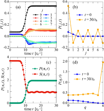
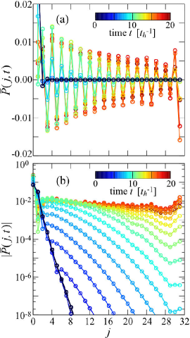
Figure 1:
(a) Time evolution of the on-site
pair-correlation function .
(b) at and .
(c) Time evolution of the pair structure factor and the spin structure factor
at .
(d) at and .
The results are calculated by the ED method for at with
, , , and .
Enhancement of the double occupancy
has been already reported in photoexcited states of the MIs Eckstein and Werner (2011); Werner et al. (2014); Yanagiya et al. (2015); Hashimoto and Ishihara (2016).
Here, we find a significant increase of the superconducting pair correlation for the on-site singlet pair
after the pulse irradiation.
Figure 1(a) shows the time evolution of the real-space pair-correlation function defined as
.
Notice that at corresponds to the double occupancy, i.e., .
We thus confirm the enhancement of by the pulse irradiation.
Surprisingly, is also enhanced significantly by the pulse irradiation and oscillates with the opposite
phases between odd and even sites.
As shown in Fig. 1(b), the pair correlation after the pulse irradiation extends to longer distances
over the cluster, while the pair correlation is essentially absent in the initial MI state before the pulse irradiation.
It is also clear that the sign of alternates between neighboring sites, similar to a density wave,
and accordingly the pair structure factor , where is the location of site ,
shows a sharp peak at [see Fig. 1(d)].
The time evolution of and the spin structure factor ,
where
and ,
is also calculated at in Fig. 1(c).
The antiferromagnetic correlation is suppressed by the pulse irradiation,
while the pair correlation
is strongly enhanced despite the fact that it is exactly zero before the pulse irradiation.
Our matrix product state calculations also find
the large enhancement of the pair correlation even for larger clusters
that cannot be treated by the ED method SM .
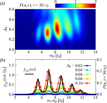
Figure 2:
(a) Contour plot of the pair structure factor at with varying
and .
(b) The GS optical spectrum is compared with as a function of
for different values of .
The results are calculated by the ED method for at , with
and .
In order to identify the optimal control parameters for the enhancement of , Fig. 2(a)
shows the contour plot of
after the pulse irradiation with different values of and .
For small , we find that the peak structure of as a function of is essentially the same
as the GS optical spectrum
,
where is the GS of with its energy and
is the current operator [see Fig. 2(b)].
This agreement is highly nontrivial and the reason will be clear below.
after the pulse irradiation is the largest at and .
We should emphasize that the enhancement of cannot be explained simply by the photodoping of carriers
into the MI or due to a dynamical phase transition induced by effectively varying the model parameters,
because there is no region in the GS phase diagram
of the Hubbard model showing large on-site pairing correlations.
Instead, the behavior of the on-site pairs in the photoinduced state shown in Fig. 1
can be understood in terms of the so-called
-pairing, a concept originally introduced by Yang Yang (1989).
In order to define the -pairing, let us first introduce the following operators:
,
and
.
Notice that () is the same as ()
except for the phase factor.
These operators satisfy the commutation relations, i.e., and .
Similarly, the total operators,
and ,
satisfy the commutation relations.
The essential property of the operators here is
that they also satisfy
with in Eq. (1).
Yang originally proposed the -pairing state ,
where is a vacuum with no electrons and is the number of pairs Yang (1989).
Yang’s -pairing state has two remarkable properties Yang (1989):
First, is an exact eigenstate of the Hubbard model with electrons,
satisfying .
Second, for ,
indicating that exhibits off-diagonal long-range order.
Notice that both Yang’s -pairing state and our photoinduced state
show similar sign-alternating characters in the pair-correlation function.
However, the photoinduced state excited from the MI state is different from the -pairing state
,
in which all electrons participate in forming pairs,
because we find numerically that at .
As a candidate of the photoinduced state showing large ,
we now consider the eigenstate generated from the lowest-weight state (LWS) for
operators.
For this purpose, it is important to notice that
. Therefore,
any eigenstate of
is also the eigenstate of
and with the eigenvalues and , respectively,
where ,
(at half-filling with the same number of up and down electrons
), and .
This is precisely the analogue to the total spin operator and its component
characterizing any eigenstate of
with . The LWS is and thus satisfies
.
Remarkably, Essler et al. have shown analytically that all the regular Bethe ansatz eigenstates of the 1D
Hubbard model are the LWSs, and the remaining eigenstates can be generated from
the LWSs by applying Essler et al. (1991, 1992, 2005).
Following them, we can construct the eigenstate having pairs from the LWS
with ( as
NL .
Yang’s -pairing state corresponds to
generated from the vacuum state with .
At half-filling, should contain electrons, and thus
we consider with
. Therefore, in this case,
, and hence
.
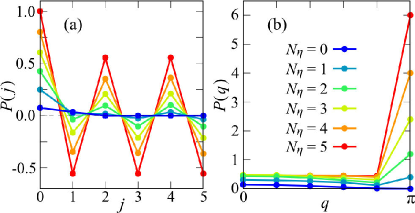
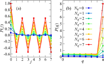
Figure 3:
(a) On-site pair-correlation function and (b) structure factor
for
at with the different number of pairs ().
is generated from the ground state of
with calculated by the ED for under PBC.
As an example, we construct from the ground state
of
with EEE , which is the LWS.
Figure 3 shows the on-site pair correlation, and ,
for
with different ’s generated from .
The sign-alternating character in and the enhancement of are clearly observed.
This is understood because
.
With increasing , crossovers to Yang’s
-pairing state at , for which is the largest.
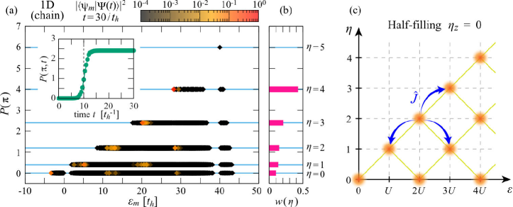
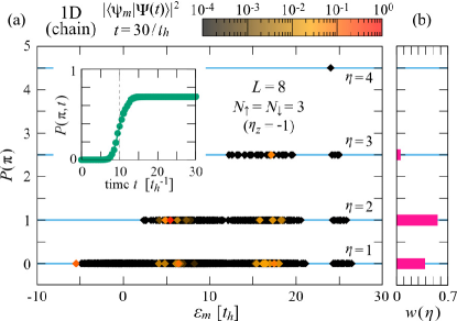
Figure 4:
(a) All eigenenergies and for the eigenstates of
the half-filled Hubbard Hamiltonian
at and under PBC.
The color of each point indicates the weight of the eigenstate
in the photoinduced state at for with ,
, ,
and .
The inset shows the time evolution of for .
(b) The total weight of over the states with the same number
of pairs in (a). Note that .
(c) Schematic figure of a “tower of states” in the photoinduced state .
The initial state before the pulse irradiation is at .
The current operator can induce the transition between states with and
,
as indicated by arrows, assuming that ,
and thus the pulse irradiation eventually excites a series of
states with nonzero and (indicated by orange spheres).
To elucidate the nature of the photoinduced state in terms of the pairs,
we calculate the eigenenergies and the structure factors
for all the eigenstates of at half-filling.
As shown in Fig. 4(a), the structure factor for each eigenstate is nicely quantized.
This is because each eigenstate is also the eigenstate of and ,
and the quantized values are given as , with , corresponding to
the number of pairs.
These quantized values are exactly the same as calculated for
in Fig. 3(b).
In Fig. 4(a), the color of each point indicates the weight of the eigenstate
in the photoinduced state
that exhibits the strong enhancement of after the pulse irradiation [see the inset of Fig. 4(a)].
We find that the state after the pulse irradiation contains the nonzero weights of the eigenstates
with finite [also see Fig. 4(b)].
This is exactly the reason for the photoinduced enhancement of .
The Hubbard model itself has the eigenstates with , and the photoinduced state
captures the weights of those eigenstates.
The process of the enhancement of is explained as follows:
Before the pulse irradiation, the initial state is the GS of
with , i.e., the singlet state Essler et al. (2005), and .
The pulse irradiation via breaks the commutation relation as
, with ,
and this transient breaking of the symmetry stirs states with different values of .
After the pulse irradiation, the Hamiltonian again satisfies the commutation relation because ,
but now contains components of , which enhance .
More precisely, in the small- limit, the external perturbation is expressed as .
We can show that the current operator is a rank-one tensor operator with the zeroth component
in terms of the operators SM . Therefore,
according to the Wigner-Eckart theorem Sakurai (1994); *MERose,
there exists the selection rule such that
only for when at half-filling.
This implies that in the linear response regime the photoinduced state can contain
the eigenstates with and the eigenenergies , assuming that
is tuned around .
This explains the good agreement between the optical spectrum and
found in Fig. 2(b).
At the second order, the photoinduced state can contain
eigenstates of with and , as well as
and and . Applying the same argument for higher orders,
-pairing eigenstates with even larger values acquire in the transient period
a finite overlap with the photoinduced state.
Considering all orders, eventually, the distribution of eigenstates in the photoinduced state
forms a “tower of states” shown schematically in Fig. 4(c),
which is indeed in good qualitative accordance with the numerical results in Fig. 4(a)
(for the analysis in the limit of , see the Supplemental Material SM ).
This also explains why the pulse irradiation is effective to induce pairs, and
the nonlinearity is essential to enhance the pair correlation.
Note that the nonlinear response is absent in the noninteracting limit,
clearly showing the importance of electron correlations.
Exactly the same argument can be applied to the two-dimensional Hubbard model on the
square lattice, and indeed we have found the large enhancement of the on-site pairing correlation in the photoinduced
state, similar to the 1D case SM .
Although the enhancement of the pair correlation is
most effective at half-filling, it remains even away from half-filling SM .
We have also examined the effect of perturbation
that breaks the symmetry, i.e., ,
and still found the enhancement of the -pairing correlation
specially in the transient period SM .
In conclusion, we have found that density-wave-like staggered superconducting correlations are induced
by photoexciting the MI ground state of the half-filled Hubbard model.
The superconductivity is due to the -pairing mechanism where the on-site singlet pairs display
off-diagonal long-range correlation with phase , the fingerprint
of the -pairing state.
We have shown that the nonlinear optical response is essential to increase the number of pairs and hence
enhance the superconducting correlation.
The -pairing states were originally introduced purely for the mathematical purpose to solve the Hubbard model
analytically, and here we have demonstrated that the pulse irradiation can bring this object into the real world
to be observed experimentally.
Finally, we note that a more realistic treatment of materials should include a coupling with other degrees of freedom
such as phonons, which introduces slow timescale dynamics in the thermalization process.
Therefore, the -pairing may be realized experimentally in a transient or prethermal regime.
The most ideal system to explore the -pairing experimentally is a cold
fermionic atom system, for which the antiferromagnetic order has been recently observed Mazurenko et al. (2017).
The authors acknowledge S. Sota, K. Seki, S. Miyakoshi, T. Oka, S. Kitamura, P. Werner, Y. Murakami, and
S. Ishihara for fruitful discussion.
This work was supported in part by Grants-in-Aid for Scientific Research from MEXT Japan under Grants
No. JP17K05523, No. JP18K13509, and No. JP18H01183.
T. S. acknowledges the Simons Foundation for financial support (Grant No. 534160).
The authors are grateful for providing computational resources of the K computer in RIKEN R-CCS through the HPCI
System Research Project (Projects No. hp140130, No. hp150140, No. hp170324, and No. hp180098).
The calculations were also performed in part on the
RIKEN supercomputer system (HOKUSAI GreatWave) at the Advanced Center for Computing and
Communications (ACCC), RIKEN.
Giannetti et al. (2016)C. Giannetti, M. Capone,
D. Fausti, M. Fabrizio, F. Parmigiani, and D. Mihailovic, Adv. Phys. 65, 58
(2016).
Fausti et al. (2011)D. Fausti, R. I. Tobey,
N. Dean, S. Kaiser, A. Dienst, M. C. Hoffmann, S. Pyon, T. Takayama,
H. Takagi, and A. Cavalleri, Science 331, 189
(2011).
Hu et al. (2014)W. Hu, S. Kaiser, D. Nicoletti, C. R. Hunt, I. Gierz, M. C. Hoffmann, M. Le Tacon, T. Loew, B. Keimer, and A. Cavalleri, Nat. Mater. 13, 705 (2014).
Kaiser et al. (2014)S. Kaiser, C. R. Hunt,
D. Nicoletti, W. Hu, I. Gierz, H. Y. Liu, M. Le Tacon, T. Loew, D. Haug, B. Keimer, and A. Cavalleri, Phys. Rev. B 89, 184516 (2014).
Mitrano et al. (2016)M. Mitrano, A. Cantaluppi,
D. Nicoletti, S. Kaiser, A. Perucchi, S. Lupi, P. Di Pietro, D. Pontiroli, M. Riccò, S. R. Clark, D. Jaksch, and A. Cavalleri, Nature (London) 530, 461 (2016).
Cantaluppi et al. (2018)A. Cantaluppi, M. Buzzi,
G. Jotzu, D. Nicoletti, M. Mitrano, D. Pontiroli, M. Riccò, A. Perucchi, P. Di Pietro, and A. Cavalleri, Nat. Phys. 14, 837 (2018).
Okamoto et al. (2010)H. Okamoto, T. Miyagoe,
K. Kobayashi, H. Uemura, H. Nishioka, H. Matsuzaki, A. Sawa, and Y. Tokura, Phys.
Rev. B 82, 060513
(2010).
Okamoto et al. (2011)H. Okamoto, T. Miyagoe,
K. Kobayashi, H. Uemura, H. Nishioka, H. Matsuzaki, A. Sawa, and Y. Tokura, Phys.
Rev. B 83, 125102
(2011).
(26)See Supplemental Material for details, which
includes Refs. Park and Light (1986); Mohankumar and Auerbach (2006); Pérez-García et al. (2007); White (1992); Schollwöck (2011); Zaletel et al. (2015); ite ; Rojo et al. (1990); Mentink et al. (2015).
De Filippis et al. (2012)G. De Filippis, V. Cataudella, E. A. Nowadnick, T. P. Devereaux, A. S. Mishchenko, and N. Nagaosa, Phys. Rev. Lett. 109, 176402 (2012).
Essler et al. (2005)F. H. Essler, H. Frahm,
F. Göhmann, A. Klümper, and V. E. Korepin, The One-Dimensional Hubbard Model (Cambridge University Press, Cambridge,
England, 2005).
Takahashi (1999)M. Takahashi, Thermodynamics of One
Dimensional Solvable Models (Cambridge University
Press, Cambridge, England, 1999).
(51)Note that is the
exact eigenstate of with the eigenenergy , where is the eigenenergy of .
Sakurai (1994)J. J. Sakurai, Modern Quantum
Mechanics (Addison-Wesley, Reading, MA, 1994).
Rose (1967)M. E. Rose, Elementary Theory of
Angular Momentum (Wiley, New
York, 1967).
Mazurenko et al. (2017)A. Mazurenko, C. S. Chiu,
G. Ji, M. F. Parsons, M. Kanasz-Nagy, R. Schmidt, F. Grusdt, E. Demler, D. Greif, and M. Greiner, Nature (London) 545, 462 (2017).
Supplemental Material
.1 Exact diagonalization method
To evaluate the state under the time-dependent Hamiltonian ,
we numerically solve the time-dependent Schrödinger equation,
(S1)
with the initial condition that , where
is the ground state of the Hamiltonian
. For this purpose,
we employ the time-dependent exact diagonalization (ED) method based on the Lanczos algorithm \citeSMPL86S,MA06S.
In this method, the time evolution with a short time step is calculated as
(S2)
where and are eigenenergies and eigenvectors of , respectively, in the corresponding Krylov
subspace generated with Lanczos iterations \citeSMHI16S,PL86S,MA06S.
In our ED calculations,
we adopt and for the time evolution, which provides results with almost machine precision accuracy.
.2 One-dimensional (1D) Hubbard model with larger : a MPS study
Method
In order to confirm the enhancement of the pair correlation in
larger systems, we also perform the time-dependent matrix-product state (MPS) \citeSMPVWetal07S
simulation for the time evolution starting from the ground state of the Hubbard model
calculated by the density-matrix
renormalization group method \citeSMWh92S, Sc11S.
For the time evolution simulation, we employ the method proposed
in Ref. \citeSMZMKetal15S, in which the time evolution operator is factorized
as a compact form of the matrix product operator (MPO) representation.
In this method, the higher order approximation for the time evolution operator
with time step are formulated by introducing the additional set of
time steps with complex numbers
in order to eliminate the unnecessary lowest order terms arisen from
the MPO factorization. The resulting error is ,
where and denote the system size and the order of the approximation,
respectively. Our calculation sets , which requires the additional time steps, i.e.,
, , ,
and , with and .
Figure S.1:
Time dependence of the on-site pair correlation function (a) and (b) logarithm of
calculated by the time-dependent MPS method for a chain of sites with OBC at .
Here, , , , and are adopted in the vector potential .
For the MPS simulation, we use the ITensor package \citeSMitensorS.
We keep the bond dimension up to to calculate the ground state of for the initial state
and for the time evolution of the system under open boundary conditions (OBC).
The time step is set to be .
Results
Figure S.1 shows the real-space on-site pair correlation function
(S3)
where and
is the number of pairs of sites separated by distance in the system of sites with OBC.
As shown in Fig. S.1,
the pair correlation extends to a longer distance gradually with time in the transient period
and shows clearly the sign-alternating feature that is characteristic of the -pairing.
The pair correlation eventually reaches to the longest distance in the system,
similar to the results shown in Figs. 1(a) and 1(b) in the main text.
.3 -pairing in the 1D Hubbard model for
As an example, Fig. 3 in the main text shows the on-site pair correlation and
of the -pairing eigenstate
(S4)
for simply because of the correspondence to Fig. 4(a) calculated for the 10 site cluster.
Here, we show supplementarily the results of and for at half-filling in Fig. S.2.
The ground state
of the Hubbard model with
is calculated
by the ED method under periodic boundary conditions (PBC).
Note that is the eigenstate of at half-filling with pairs.
As shown in Fig. S.2, the density-wave-like pair correlation is largest for .
Figure S.2:
(a) On-site pair correlation function and (b) on-site pair structure factor
for the half-filled -paring eigenstate
at with the different number of pairs ().
is generated from the ground state of the Hubbard
model with calculated by the ED method for under PBC.
.4 Hubbard model on the square lattice
In the main text, we focus on the 1D Hubbard model to demonstrate that the strong superconducting correlation
can be induced in the Mott insulator (MI) by the pulse irradiation, and show that the origin of this
superconductivity is
due to the -pairing mechanism.
Here, we show that exactly the same conclusion can be reached for the two-dimensional (2D) Hubbard model on the
square lattice with only nearest neighbor hoppings.
Model and operators
The 2D Hubbard model is described by the following Hamiltonian:
(S5)
where the sum runs over all pairs of nearest neighbor sites and on the square lattice.
Similarly to the 1D case, the total operators and
are defined in terms of
the local operators
,
and
, where the location of
site is given as and is the unit vector along the direction.
These operators satisfy the commutation relations.
We can also show that and
. Therefore,
any eigenstate of the Hubbard model can be chosen
also to be an eigenstate of
and with the eigenvalues and , respectively, where
can take and , assuming that the number
of up electrons and the number of down electrons are the same and (even)
is the total number of sites.
At half-filling with , the eigenstates are characterized with and ,
and the ground state of the Hubbard model is .
The real-space on-site pair correlation function for the time-evolved state is defined as
(S6)
where and the pair structure factor
in the momentum space is given as
(S7)
Noticing that , at is
(S8)
(S9)
The pair structure factor for is thus
.
Any eigenstate can be constructed from the LWS by repeatedly
applying because
(S10)
Since by definition,
the LWS contains no pairs and
.
Each time that is applied from the LWS, the number of pairs increases by one, and
the maximum number of pairs is obtained when (i.e., half-filling) for a given , where
and the number of pairs is .
The time-dependent external field is introduced in Eq. (S5) by
with the time-dependent vector potential pointing along the diagonal direction
and given in the main text.
The current operator along a direction () is defined as
(S11)
where is the creation operator of an electron at the site located at
with spin .
We can now show that
(S12)
(S13)
where
(S14)
and
(S15)
Therefore, with is a rank-one tensor operator in terms of operators.
In particular, the current operator is a rank-one tensor operator with and hence
there is the following selection rule: only for
when \citeSMJJSakuraiS,MERoseS.
We also note that
is a rank-one tensor operator with , while
is a rank-zero tensor operator, i.e.,
a scalar operator.
Although here we consider the 2D case, the extension to other spatial dimensions is straightforward.
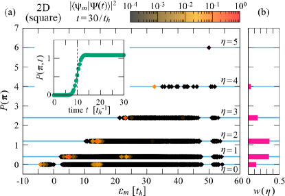
Figure S.3:
(a) All eigenenergies and [] for the eigenstates
of the half-filled Hubbard model on a
cluster with PBC at .
The color of each point (diamond) indicates the weight of the eigenstate
in the photoinduced state at . Here, ,
, , and are adopted in the vector potential .
When the eigenstates are degenerate, the color indicates the sum of over these degenerate
states.
The time evolution of for is also shown in the inset.
(b) The total weight of over the states that have the same number
of pairs, and thus . The parameters are the same as in (a).
Results
As shown above,
any eigenstate of can be chosen to be
an eigenstate of and .
Figure S.3(a) shows all the eigenenergies of
and the corresponding pair structure factors
at on a cluster with PBC at half-filling.
Indeed, as in the 1D case, is quantized
as , where corresponds to the number of pairs.
As shown in Fig S.3(b), the photoinduced state after the pulse irradiation displays
nonzero overlaps with the eigenstates of with .
This is responsible for the large enhancement of in the photoinduced state
[see the inset of Fig. S.3(a)].
Since the current operator is a rank-one tensor operator, we can again observe in Fig. S.3(a)
a “tower of states” structure of the eigenstates contributing
to the photoinduced state with large weights
.
.5 1D Hubbard model away from half-filling
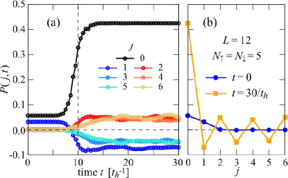
We also examine the behavior of the photoinduced states in the 1D Hubbard model away from half-filling.
Figure S.4 shows the time evolution of the pair correlation function calculated by the ED method
for with (10 electrons in total) under PBC.
Although the magnitude of is smaller than that for the case of half-filling, clearly shows a pair density wave
like oscillation with the correlation extended up to the longest distance of the cluster.
Therefore, the -pairing correlation is induced in the photoexcited state in the Hubbard model
even away from half-filling.
Figure S.4:
(a) Time evolution of the on-site pair correlation function with hole doping.
(b) at (blue circles) and (orange squares).
The results are calculated by the ED method for and at with
, , , and .
To elucidate the nature of the photoinduced state in terms of the pairs,
we calculate the eigenenergies and the structure factors
for all the eigenstates of the 1D Hubbard model with hole-doping.
Figure S.5 shows the results for with (6 electrons in total) under PBC.
As shown in Fig. S.5(a), the structure factor for each eigenstate is nicely quantized.
This is because each eigenstate away from half-filling is also the eigenstate of
and .
The quantized values are given as
(S16)
with
and .
Note that (no pair state) is characterized by the state with because and this state
is the LWS.
In Fig. S.5(a), the color of each point indicates the weight of the eigenstate
in the photoinduced state that exhibits the enhancement of after the pulse irradiation [see the inset of Fig S.5(a)].
We find that the state after the pulse irradiation contains the nonzero weights of the eigenstates
with finite [also see Fig. S.5(b)].
Therefore, the reason for the enhancement of is
the same as in the case at half-filling.
Figure S.5:
(a) All eigenenergies and for the eigenstates of
the hole-doped 1D Hubbard model at for under PBC with
electrons.
The color of each point (diamond) indicates the weight of the eigenstate
in the photoinduced state at . Here, ,
, , and are adopted in the vector potential .
When the eigenstates are degenerate, the color indicates the sum of over these degenerate
states.
The time evolution of for is also shown in the inset.
(b) The total weight of over the states that have the same
eigenvalue of ,
and thus .
The parameters are the same as in (a).
Note that the number of pairs is for this hole-doped case.
However, the distribution of the weight after the pulse irradiation in Fig. S.5(a) is
qualitatively different from that in the case at half-filling shown in Fig. 4(a) in the main text.
For example, there is the finite contribution to the weight from the eigenstates
with around ,
which is absent at half-filling.
This is explained by the different selection rules of the current operator for the half-filled ()
and hole-doped () states.
As mentioned in the main text and also in Sec. .4,
is a rank-one tensor operator with the zeroth component in terms of the operators.
Hence, from the Wigner–Eckart theorem \citeSMJJSakuraiS,MERoseS, the selection rule of
is given as
(S17)
with the 3-symbol.
The 3-symbol is zero unless and are satisfied.
Therefore, for when
for the hole-doped states. The result in Fig. S.5(a) follows this selection rule.
However, when for the half-filled state, the nonzero 3-symbol must satisfy
the additional rule: .
Therefore, the excitation to the states with is not induced by at half-filling
(), and only for .
The results at half-filling in Fig. 4(a) in the main text and Fig. S.3(a) follow this selection rule.
.6 Perturbation analysis in the limit of large pulse width
In the large pulse width limit, i.e., , the time-dependent vector
potential is given as .
Let us denote the time-dependent Hamiltonian with the time-dependent external field as
(S18)
where is the time-independent part of the Hamiltonian given by, e.g.,
Eq. (1) in the main text
and is the time-dependent part of the Hamiltonian given as
(S19)
Because becomes a periodic function of in the limit ,
can be expanded using Bessel functions of the first kind
(: integer) \citeSMKA16S, i.e.,
(S20)
where
(S21)
Here we set .
It is important to notice in Eqs. (S20) and (S21)
that the operator in the even terms is
the kinetic (rank-zero tensor) operator, i.e.,
(S22)
while the operator in the odd terms is
the current (rank-one tensor) operator, i.e.,
(S23)
as defined also in the main text.
A time-dependent state governed by can be expanded as
(S24)
where () are
the th eigenstate of
with the eigenenergy . For simplicity,
we assume that the ground state is not degenerate with .
By using the time-dependent perturbation theory,
the coefficient is obtained as the sum
over terms of the th order expansion in terms of :
(S25)
Assuming that the initial state at time
is the ground state
of , is given as
It is now obvious from the delta function in Eq. (S29)
that the coefficients for
can be nonzero only if ,
suggesting that the excitations are allowed only to states with the excitation energy that is
an integer multiple of .
This nicely explains the energy dependence found in Fig. 4(a) in the main text and Fig. S.3(a)
for half-filling and also in Fig. S.5(a) away from half-filling.
For example, if (: integer),
should involve the odd number of
excitations induced by the current operator .
In the case of half-filling, combining this with the selection rule in Eq. (S17)
yields that the odd excitations are
possible if and only if .
Similarly, the even excitations are possible if and only if
the at half-filling.
These are in accordance with the “tower of states” structure shown schematically
in Fig. 4(c) in the main text.
.7 1D Hubbard model with the next-nearest-neighbor hopping
In this and the next sections, we investigate the pair correlations when the commutation relations, e.g.
, are broken
in the Mott-Hubbard system.
First, we consider the 1D Hubbard model with the next-nearest-neighbor (NNN) hopping described by
, where is given by
Eq. (1) in the main text and
(S30)
is the NNN hopping term. Because
, the Hamiltonian breaks the commutation relations.
Figure S.6 shows the time dependence of the pair correlation functions for the photoexcited state
with different values of calculated by the ED method for under PBC.
As in the main text, the time-dependent external field is introduced via the Peierls phase through
the time-dependent vector potential ,
where the Peierls phase for the NNN hopping is given as
and the form of is described in the main text.
Although the commutation relations are broken when is finite in ,
we find the enhancement of the pair correlation functions, specially during the transient period, with
the -pairing like sign-alternating oscillation [see Fig. S.6(b)].
Note that, unlike in the case of , is no longer conserved after the pulse irradiation
because of .
With increasing , at becomes suppressed and eventually show no longer range correlation
after the pulse irradiation [see Fig. S.6(c)].
Therefore, we conclude that the photoinduced states still show the robust -pairing correlations transiently as long as
the NNN hopping is small, although the large NNN hopping is unfavorable for the photoinduced -pairing.
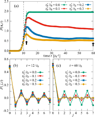
Figure S.6:
(a) Time evolution of the pair structure factor in the 1D Hubbard model with the NNN hopping
at half-filling.
Two arrows indicate the time, and , at which the
real-space pair correlation function is calculated in (b) and (c), respectively.
Note that in (b) is within the transient period.
The results are calculated by the ED method for (PBC) at with , ,
, and for the time-dependent vector potential .
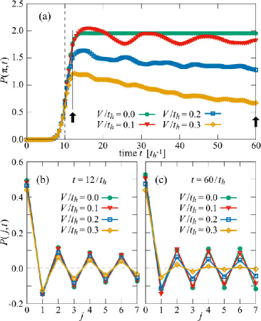
Figure S.7:
(a) Time evolution of the pair structure factor in the 1D Hubbard model with the
nearest-neighbor Coulomb interaction at half-filling.
Two arrows indicate the time, and , at which the real-space
pair correlation function is calculated in (b) and (c), respectively.
Note that in (b) is within the transient period.
The results are calculated by the ED method for (PBC) at with ,
, , and for the time-dependent vector potential .
.8 1D Hubbard model with the nearest-neighbor Coulomb interaction
In addition, we examine the influence of the nearest-neighbor Coulomb interaction on the pair correlation
in the photoinduced state.
The model considered here is the 1D extended Hubbard model described by
, where
the intersite Coulomb interaction term is given as
(S31)
Because , the Hamiltonian
breaks the commutation relations.
Figure S.7 shows the time dependence of the pair correlation functions
for the photoexcited state with different values of
calculated by the ED method for
under PBC. The time-dependent external field is introduced exactly in the same form described in the main text.
Although the commutation relations are broken when is finite in ,
we find the enhancement of the pair correlation functions at least in the transient period of the pulse irradiation,
clearly exhibiting the -pairing like sign-alternating oscillation [see Fig. S.7(b)].
However, when is relatively large, the pair correlation is quickly suppressed with increasing after the
pulse irradiation [see Fig. S.7(c)].
Therefore, we conclude that the photoexcited state can still show the robust pair correlation in the transient period,
but the strong intersite Coulomb interaction can eventually disturb the photoinduced -pairing completely
for large .
.9 Other related studies for -pairing
In nonequilibrium contexts, possible realization of the -paring state has also been proposed in the
repulsive Hubbard systems with the harmonic trapping potential \citeSMRRBetal08S
and with the dissipative coupling \citeSMBBPetal13S.
However, unlike these studies, our mechanism shown here is based on the selection rule derived from
the commutation relation between the pair and current operators, and therefore
provides a completely different pathway of pair generation.
In the attractive Hubbard model, Kitamura and Aoki have investigated the -pairing state induced by the periodically
driven field \citeSMKA16S.
Based on the Floquet formalism for the effective model in the strong coupling limit,
composed of the pair hopping term and the nearest-neighbor pair repulsion,
which can be mapped onto a Heisenberg like model \citeSMRSB90S,
they have shown that
the -paring state can be induced from the -wave superconducting state
by varying the effective model parameters \citeSMKA16S.
However, the corresponding argument cannot be applied to the repulsive
Hubbard model \citeSMMBE15S,
and thus our mechanism also differs from their suggestion.