Upper magnetic field in superconducting Dirac semi-metal

Abstract

Temperature dependence of the upper critical field $H_{c2}$ of the Dirac semi - metal (DSM) with phonon mediated pairing is considered within semi - classical approximation. The low temperature dependence deviates from conventional BCS superconductor with parabolic dispersion relationWHH even for large adiabaticity parameter, $\gamma=\mu/\left(\hbar\Omega\right)$., where $\mu$ is the chemical potential and $\Omega$ - Debye frequency. In particular the ”reduced field”, ratio of zero temperature $H_{c2}$ to derivative at critical temperature, $h^{\ast}=H_{c2}\left(0\right)/\left(-T\frac{dH_{c2}}{dT}\right)|_{T_{c}}$, depends on $\gamma$ and can be extended beyond the adiabatic limit. The reduced magnetic field ratio is universal (independent of the chemical potential, interaction strength etc.) and smaller than the Werthamer ratio for clean superconductors: $h^{\ast}=0.55$ for DSM, $h^{\ast}\left(0\right)=0.69$ for parabolic band. The results are in good agreement compared with recent experiments on $TaP$.

I Introduction

Recently a large new class of 2D (including purely 2D materials like graphene and surfaces of ”topological insulators”) and 3D multi-band materials with qualitatively different band structure (Dirac point) near the Fermi level was discovered. Unlike in conventional semi-metals with several quasiparticle and hole bands, the Dirac points occur due to the band inversion near the Fermi level. In many of them (sometimes under pressure) superconductivity was observed at low temperatures Geim ; superWSM2D ; superWSM3D ; Cao ; PdTe2 ; Hf . Dirac semi-metals (DSM) are characterized by linear dispersion relation, and the chemical potential is tunable and small. More importantly for the pairing of the quasiparticles by phonons leading to ”conventional” superconductivity is that their inter - band tunneling is dominant frontiers ; JCM15 .

In type I DSM, the band inversion results in Dirac points in low-energy excitations being anisotropic massless ”relativistic” fermions (Dirac cone in dispersion relation, $\varepsilon=vp$). They exhibit several remarkable properties like the chiral magnetic effect related to the chiral anomaly in particle physics and tend to form the s-wave superconductivity DasSarma ; FuBerg ; Shapiro14 ; ruslan of the second kind (recently discovered type-II DSMs Goerbig1 ; Soluyanov with tilted cones and nearly flat bands tend to exhibit superconductivity of first kind PdTe2 ).

Magnetic properties of the DSM turned superconductor of the second kind are typically standard. The upper critical magnetic field $H_{c2}\left(T\right)$ was measured in wide range of temperatures for different DSM and it demonstrates behavior typical for vortex matter. In particular in layered DSM (that possess relatively large Ginzburg number $Gi$) $MoTe_{2}$ MoTe2 the thermal fluctuations effects are observed in the vicinity of the critical temperature $T_{c}$ Rosenstein18 ; strongfield ; koshelev . The general theory based in Ginzburg - Landau approach (that is insensitive to the microscopic details distinguishing between metal with parabolic bands, DSM of high $T_{c}$ unconventional superconductors) is applicable for most of the observed features.

However it was noticed very recently that the low temperature dependence of the $H_{c2}\left(T\right)$ curve in some DSM, like ZrTe $ZrTe_{5}$, CdAs $Cd_{3}As_{2}$ andTaP $TaP$, significantly deviate from that predicted by the quasi-classical microscopic theory for conventional parabolic band superconductors Gorkov ; WHH ; Bulaevsky . The low temperature limit is beyond the universality range of the GL approach and is sensitive to the ”microscopic details”, especially when the inter-band tunneling is present. The deviations were discussed in literature for superconductors that have large gyromagnetic ratioChandrasekhar , but this is clearly not the case here. Therefore it is important to extend the original Werhamer-Helfand-Hohenberg WHH theory of the upper critical field to the case of multi - band DSM with large tunneling between the valleys koshelev ; Rosenstein18 ; Rosenstein17 .

This is the purpose of the present work. The quasi-classic theory of the phonon - mediated pairing in magnetic fields in DSM is developed in wide range of temperatures and adiabatic parameters. In particular the reduced magnetic field at zero temperature defined by $h^{\ast}=H_{c2}\left(0\right)/\left(-TdH_{c2}/dT\right)|_{T_{c}}$ for different adiabaticity ratio $\gamma=\mu/\hbar\Omega$ ($\mu$ is the chemical potential, while $\Omega$ is Debye frequency) is calculated. Even within the BCS limit $\gamma\rightarrow\infty$ the reduced magnetic field is smaller than the conventional WHH WHH (extended to the layered system by Bulaevsky Bulaevsky with the magnetic field directed perpendicular to the layers) value $h_{WWH}^{\ast}=0.69$.

In addition, since in DSM the adiabaticity ratio in Weyl semi-metals is relatively small, an important additional issue is the role of the retardation effects of the phonon mediated pairing. Within the semiclassical approach one can approach moderately adiabatic case, $\gamma\simeq 1$.

II Pairing in the DSM under magnetic field

II.1 Hamiltonian

Dirac material typically possesses several sublattices. We exemplify the effect of the DSM band structure on superconductivity using the simplest model with just two sublattices denoted by $\alpha=1,2$. The effective electron-electron attraction due to the electron - phonon coupling overcomes the Coulomb repulsion and induces pairing. Typically in DSM there are numerous bands. We assume that different valleys are paired independently and drop all the valley indices (including chirality, multiplying the density of states by $2N_{f}$). To simplify notations, we therefore consider just one spinor (left, for definiteness), the following Weyl HamiltonianJCM15 , Wang .

$$K=\int_{\mathbf{r}}\psi_{\alpha}^{s\dagger}\left(\mathbf{r}\right)\left\{-i\hbar v\left(D_{x}\sigma_{\alpha\beta}^{x}+D_{y}\sigma_{\alpha\beta}^{y}\right)-i\hbar v_{z}D_{z}\sigma_{\alpha\beta}^{z}-\mu\delta_{\alpha\beta}\right\}\psi_{\beta}^{s}\left(\mathbf{r}\right).$$ (1)

Here $v$ is Fermi velocity assumed isotropic in the plane $x-y$ perpendicular to the applied magnetic field, $v_{z}$ is the velocity in magnetic field direction. Chemical potential is denoted by $\mu$. Pauli matrices $\sigma$ operate in the sublattice space (the indices $\alpha,\beta$ will be termed the pseudo-spin projections) and $s$ is spin projection. Magnetic field appears in the covariant derivatives via the vector potential, $D_{i}=\nabla^{i}-i\frac{e}{\hbar c}A_{i}$. Here $\mathbf{A}$ is the vector potential.

Further we assume the local density - density interaction Hamiltonian Abrikosov ,

$$V=\frac{g^{2}}{2}\int_{\mathbf{r}}\psi_{\alpha}^{+\uparrow}\left(\mathbf{r}\right)\psi_{\alpha}^{\downarrow}\left(\mathbf{r}\right)\psi_{\beta}^{\downarrow+}\left(\mathbf{r}\right)\psi_{\beta}^{\uparrow}\left(\mathbf{r}\right)\text{,}$$ (2)

ignoring the Coulomb repulsion (that as usual is accounted for by a pseudopotential, so that $g$ is the electron - phonon coupling). It is important that the interaction has a cutoff Debye frequency $\Omega$, so that it is active in an energy shell of width $2\hbar\Omega$ around the Fermi level Abrikosov .

II.2 Matsubara Green’s functions and Gor’kov equations

Finite temperature properties of the superconducting condensate are described by the normal and the anomalous Matsubara Green’s functions Abrikosov (GF),

$$G_{\alpha\beta}^{ts}\left(\mathbf{r}\tau,\mathbf{r}^{\prime}\tau^{\prime}\right) = -\left\langle T\psi_{\alpha}^{t}\left(\mathbf{r}\tau\right)\psi_{\beta}^{\dagger s}\left(\mathbf{r}^{\prime}\tau^{\prime}\right)\right\rangle;F_{\alpha\beta}^{ts}\left(\mathbf{r}\tau,\mathbf{r}^{\prime}\tau^{\prime}\right)=\left\langle T\psi_{\alpha}^{t}\left(\mathbf{r}\tau\right)\psi_{\beta}^{s}\left(\mathbf{r}^{\prime}\tau^{\prime}\right)\right\rangle;$$ (3)

$$F_{\alpha\beta}^{+ts}\left(\mathbf{r}\tau,\mathbf{r}^{\prime}\tau^{\prime}\right) = \left\langle T\psi_{\alpha}^{\dagger t}\left(\mathbf{r}\tau\right)\psi_{\beta}^{\dagger s}\left(\mathbf{r}^{\prime}\tau^{\prime}\right)\right\rangle,$$

with the spin Ansatz

$$G_{\alpha\beta}^{ts}\left(\mathbf{r}\tau,\mathbf{r}^{\prime}\tau^{\prime}\right) = \delta^{ts}G_{\alpha\beta}\left(\mathbf{r,r}^{\prime},\tau-\tau^{\prime}\right);F_{\alpha\beta}^{ts}\left(\mathbf{r}\tau,\mathbf{r}^{\prime}\tau^{\prime}\right)=-\varepsilon^{ts}F_{\alpha\beta}\left(\mathbf{r,r}^{\prime},\tau-\tau^{\prime}\right);$$ (4)

$$F_{\alpha\beta}^{+ts}\left(\mathbf{r}\tau,\mathbf{r}^{\prime}\tau^{\prime}\right) = \varepsilon^{ts}F_{\alpha\beta}^{+}\left(\mathbf{r,r}^{\prime},\tau-\tau^{\prime}\right)\text{.}$$

Here the Plank constant is set to $\hbar=1$. Using the Fourier transform,

$$G_{\gamma\kappa}\left(\mathbf{r},\tau\right)=T\sum\nolimits_{s}\exp\left[-i\omega_{s}\tau\right]G_{\gamma\kappa}\left(\omega,\mathbf{r}\right)\text{,}$$ (5)

with fermionic Matsubara frequencies, $\omega_{s}=2\pi T\left(s+1/2\right)$, one obtains from equations of operator motion the set of Gor’kov equations, see JCM15 ,Rosenstein generalized to include magnetic field:

$$\left(i\omega+\mu\right)G_{\gamma\kappa}\left(\mathbf{r,r}^{\prime},\omega\right)+i\ vD_{\mathbf{r}}^{i}\sigma_{\gamma\beta}^{i}G_{\beta\kappa}\left(\mathbf{r,r}^{\prime},\omega\right)+\Delta_{\alpha\gamma}\left(\mathbf{r,}0\right)F_{\alpha\kappa}^{+}\left(\mathbf{r,r}^{\prime},\omega\right) = \delta^{\gamma\kappa}\delta\left(\mathbf{r-r}^{\prime}\right);$$

$$\left(-i\omega+\mu\right)F_{\gamma\kappa}^{+}\left(\mathbf{r},\mathbf{r}^{\prime},\omega\right)-ivD_{\mathbf{r}}^{i}\sigma_{\alpha\gamma}^{i}F_{\alpha\kappa}^{+}\left(\mathbf{r},\mathbf{r}^{\prime},\omega\right)-\Delta_{\alpha\gamma}^{\ast}\left(\mathbf{r},0\right)G_{\alpha\kappa}\left(\mathbf{r},\mathbf{r}^{\prime},\omega\right) = 0\text{.}$$ (6)

It will be shown that the singlet pairing pseudo-spin Ansatz, $\Delta_{\alpha\gamma}\equiv\sigma_{\alpha\gamma}^{x}\Delta$, obeys the Pauli principle. The gap function consequently reads: $\Delta=\frac{1}{2}Tr\left[\sigma^{x}\widehat{\Delta}\right]$. Notice, that in contrast to conventional metals with parabolic dispersion law, in the case of the Weyl semi - metals the second Gor’kov equation, Eq.(6), contains transposed Pauli matrices for isospins. The applicability of the mean field approach in a purely 2D model have been widely discussed RMP since (logarithmic) infrared divergences appear in corrections to the approximation. The corrections of the long range charge density waves instability are assumed to be cut off by the finite size of the sample, etc.

III The transition line in H-T plane

Near the normal-to-superconducting transition line the gap $\Delta$ is small and the set of the Gor’kov equations (6) can be linearized. We consider here the 2D case neglecting velocity in magnetic field direction. More general case will be discussed below. In this case the gap equation describing the critical curve $H_{c2}\left(T\right)$ has  the form, see Rosenstein for details,

$$\Delta\left(\mathbf{r}\right) = \frac{g^{2}}{2}T\sum\nolimits_{\omega}\int_{\mathbf{r}^{\prime}}\Delta^{\ast}\left(\mathbf{r}^{\prime}\right)\sigma_{\kappa\beta}^{x}G_{\beta\gamma}^{2}\left(\mathbf{r^{\prime},r}\right)\sigma_{\gamma\alpha}^{x}G_{\alpha\kappa}^{1}\left(\mathbf{r,r}^{\prime}\right)$$ (7)

$$= g^{2}\sum\nolimits_{\omega}\int_{\mathbf{r}^{\prime}}\Delta^{\ast}\left(\mathbf{r}^{\prime}\right)\left(\begin{array}[]{c}G_{22}^{2}\left(\mathbf{r^{\prime},r}\right)G_{1\mathbf{1}}^{1}\left(\mathbf{r,r}^{\prime}\right)+G_{11}^{2}\left(\mathbf{r^{\prime},r}\right)G_{2\mathbf{2}}^{1}\left(\mathbf{r,r}^{\prime}\right)\\ +G_{12}^{2}\left(\mathbf{r^{\prime},r}\right)G_{12}^{1}\left(\mathbf{r,r}^{\prime}\right)+G_{21}^{2}\left(\mathbf{r^{\prime},r}\right)G_{2\mathbf{1}}^{1}\left(\mathbf{r,r}^{\prime}\right)\end{array}\right)\text{.}$$ (10)

Here the normal GF is obtained from,

$$\left[\ iv\mathbf{D}_{\mathbf{r}}\cdot\mathbf{\sigma}_{\gamma\beta}+\left(i\omega+\mu\right)\delta_{\gamma\beta}\right]G_{\beta\kappa}^{1}\left(\mathbf{r,r}^{\prime}\right)=\delta^{\gamma\kappa}\delta\left(\mathbf{r-r}^{\prime}\right)\text{,}$$ (11)

while a quantity$\ G_{\beta\gamma}^{2}$ (an auxiliary function associated with $G$ via a product of an axis reflection and time reversal) obeys a different equations:

$$\left[-iv\mathbf{D}_{\mathbf{r}}\cdot\mathbf{\sigma}_{\gamma\beta}^{t}+\left(-i\omega+\mu\right)\delta_{\gamma\beta}\right]G_{\beta\kappa}^{2}\left(\mathbf{r}^{\prime}\mathbf{,r}\right)=\delta^{\gamma\kappa}\delta\left(\mathbf{r-r}^{\prime}\right)\text{.}$$ (12)

Here $\mathbf{\sigma}^{t}$ is the transposed Pauli matrix that replaces $\mathbf{\sigma}$ in the customary normal state Weyl equation for left movers, Eq.(11).

In the uniform magnetic field the GF can be written in the symmetric gauge, $\mathbf{A=}\frac{1}{2}\mathbf{H\times r}$, in the following form:

$$G_{\beta\kappa}^{1}\left(\mathbf{r},\mathbf{r}^{\prime}\right) = \exp\left[-i\frac{xy^{\prime}-yx^{\prime}}{2l^{2}}\right]g_{\beta\kappa}^{1}\left(\mathbf{r-r}^{\prime}\right);$$ (13)

$$G_{\beta\kappa}^{2}\left(\mathbf{r}^{\prime},\mathbf{r}\right) = \exp\left[-i\frac{xy^{\prime}-yx^{\prime}}{2l^{2}}\right]g_{\beta\kappa}^{2}\left(\mathbf{r}^{\prime}\mathbf{-r}\right)\text{.}$$

Here $l^{2}=c/eH$ is the magnetic length. This phase Ansatz indeed works. Substituting it into Eq.(11) and Eq.(12) respectively, the variables separate. It reads,

$$L_{\gamma\beta}^{1}g_{\beta\kappa}^{1}\left(\mathbf{r-r}^{\prime}\right)=\delta^{\gamma\kappa}\delta\left(\mathbf{r-r}^{\prime}\right);L_{\gamma\beta}^{2}g_{0\beta\kappa}^{2}\left(\mathbf{r-r}^{\prime}\right)=\delta^{\gamma\kappa}\delta\left(\mathbf{r-r}^{\prime}\right)\text{,}$$ (14)

where $L_{\gamma\beta}^{1}=\left[\left(i\omega+\mu\right)\delta_{\gamma\beta}+\left(-iv\sigma_{\gamma\beta}^{i}\ \nabla_{r}^{i}\right)\right]$ , $L_{\gamma\beta}^{2}=\left[\left(-i\omega+\mu\right)\delta_{\gamma\beta}-iv\sigma_{\gamma\beta}^{it}\nabla_{r}^{i}\right]$.

Solutions of these equations gives;

$$g_{22}^{1}\left(\mathbf{p}\right) = z^{\ast-1}\left(i\omega+\mu\right);\text{ \ }g_{12}^{1}\left(\mathbf{p}\right)=-z^{\ast-1}v\left(p_{x}-ip_{y}\right);g_{11}^{1}\left(\mathbf{p}\right)=z^{\ast-1}\left(i\omega+\mu\right);$$ (15)

$$\text{ }g_{21}^{1}\left(\mathbf{p}\right) = -z^{\ast-1}v\left(p_{x}+ip_{y}\right);g_{11}^{2}\left(\mathbf{p}\right)\ =z^{-1}\ \left(-i\omega+\mu\right);\text{ }g_{12}^{2}\left(\mathbf{p}\right)=-z^{-1}v\left(p_{x}+ip_{y}\right);$$

$$g_{22}^{2}\left(\mathbf{p}\right) = z^{-1}\left(-i\omega+\mu\right);\text{ \ }g_{21}^{2}\left(\mathbf{p}\right)=-z^{-1}v\left(p_{x}-ip_{y}\right)\ ;$$

where $z=\left(-i\omega+\mu\right)^{2}-\left(vp\right)^{2}$ and $p$ denote quasi-momentum.

Substituting the phase factors of GF from Eq.(13) into the gap equation, Eq.(7), one obtains:

$$\Delta\left(\mathbf{r}\right)=g^{2}T\sum\nolimits_{\omega}\int_{\mathbf{r}^{\prime}}\exp\left[\ i\frac{\left[\mathbf{r\times\rho}\right]}{l^{2}}\right]\Delta^{\ast}\left(\mathbf{r}^{\prime}\right)\left(\begin{array}[]{c}g_{22}^{2}\left(\mathbf{-\rho}\right)g_{11}^{1}\left(\mathbf{\rho}\right)+g_{11}^{2}\left(\mathbf{-\rho}\right)g_{22}^{1}\left(\mathbf{\rho}\right)\\ +g_{12}^{2}\left(\mathbf{-\rho}\right)g_{12}^{1}\left(\mathbf{\rho}\right)+g_{21}^{2}\left(\mathbf{-\rho}\right)g_{21}^{1}\left(\mathbf{\rho}\right)\end{array}\right),$$ (16)

where $\mathbf{\rho}\mathbf{=}\mathbf{r-r}^{\prime}$. Looking for the gap function $\Delta\left(\mathbf{r}\right)$ in the formIndia $\Delta\left(\mathbf{r}\right)=\Delta\exp\left(-\frac{r^{2}}{2l^{2}}\right)$, one obtains after Fourier transformation.

$$1=g^{2}T\sum\nolimits_{\omega}\int\mathbf{d}^{2}\mathbf{\rho}\exp\left[\ i\frac{\left[\mathbf{r\times\rho}\right]-\mathbf{r\rho}}{l^{2}}\right]\exp\left(-\frac{\mathbf{\rho}^{2}}{2l^{2}}\right)\int\frac{d^{2}\mathbf{p}d^{2}\mathbf{q}}{\left(2\pi\right)^{4}}e^{i\mathbf{q\rho}}S\left(\mathbf{p,q}\right),$$ (17)

where

$$S\left(\mathbf{p,q}\right)=\frac{2\left[\omega^{2}+\mu^{2}+v^{2}\left(\mathbf{p-q}\right)\cdot\mathbf{p}\right]}{\left[\left(-i\omega+\mu\right)^{2}-v^{2}\left(\mathbf{p-q}\right)^{2}\right]\left[\left(i\omega+\mu\right)^{2}-v^{2}\mathbf{p}^{2}\right]}$$ (18)

In the polar coordinates Eq.18 has the form

$$1 = \frac{2g^{2}T}{v^{4}\left(2\pi\right)^{2}}\sum\nolimits_{\omega}\int\rho d\rho d\Theta d\varepsilon_{q}\ d\varepsilon_{p}d\psi\exp\left[\ \frac{ir\rho\sin\Theta-r\rho\cos\Theta}{l^{2}}-\frac{\rho^{2}}{2l^{2}}\right]\cdot$$

$$\cdot J_{0}\left(\frac{\varepsilon_{q}\rho}{v}\right)\varepsilon_{q}\varepsilon_{p}\frac{\omega^{2}+\mu^{2}+\varepsilon_{p}^{2}\mathbf{-}\varepsilon_{p}\varepsilon_{q}\cos\psi}{\left[\left(-i\omega+\mu\right)^{2}-\left(\varepsilon_{p}^{2}-2\varepsilon_{p}\varepsilon_{q}\cos\psi+\varepsilon_{q}^{2}\right)\right]\left[\left(i\omega+\mu\right)^{2}-\varepsilon_{p}^{2}\right]}.\$$

Here $\Theta$ is the angle between vectors $\mathbf{r}$ and $\mathbf{\rho}$ while $\psi$ is the angle between momentum $\mathbf{p}$ and $\mathbf{q}$, $vp=\varepsilon_{p};vq=\varepsilon_{q},$ $J_{0}(z)$ is the Bessel function.

Usually within the BCS approach, the interaction is approximated not just by a contact in space and a step function - like cutoff,

$$\mu-\hbar\Omega<\varepsilon_{p}<\mu+\hbar\Omega\text{,}$$ (20)

Therefore the in Eq.(22) is restricted. This is unphysical since the step function dependence is just an approximation of a more realistic second order effective electron interaction due to phonon exchange.

Neglecting the dispersion of the optical phonon, the sharp cutoff will be replaced by the Lorenzian function

$$f\left(\varepsilon_{p}\right)=\frac{\Omega^{2}}{\Omega^{2}+\left(\varepsilon_{p}-\mu\right)^{2}}\text{.}$$ (21)

Performing integral Gradshtein ,koshelev over angle $\Theta$ and $\rho$ one obtains the coexistence curve at $H-T$ plane in reduced variables with barred energies denoting division by temperature $T$: $\left(\overline{\mu}=\mu/T,\overline{\omega}=\omega/T,\overline{\varepsilon}_{p,q}=\varepsilon_{p.q}/T\right)$

$$\frac{1}{\lambda}=\frac{2\chi}{\overline{\mu}}\sum\nolimits_{\omega}\int d\overline{\varepsilon}_{q}d\overline{\varepsilon}_{p}d\psi\frac{f\left(\overline{\varepsilon}_{p}\right)\overline{\varepsilon}_{q}\overline{\varepsilon}_{p}\exp\left[-\chi\overline{\varepsilon}_{q}^{2}\right]\left(\overline{\omega}^{2}+\overline{\mu}^{2}+\overline{\varepsilon}_{p}^{2}\mathbf{-}\overline{\varepsilon}_{q}\overline{\varepsilon}_{p}\cos\psi\right)}{\left[\left(-i\overline{\omega}+\overline{\mu}\right)^{2}-\left(\overline{\varepsilon}_{p}^{2}+\overline{\varepsilon}_{q}^{2}-2\overline{\varepsilon}_{p}\overline{\varepsilon}_{q}\cos\psi\right)\right]\left[\left(i\overline{\omega}+\overline{\mu}\right)^{2}-\overline{\varepsilon}_{p}^{2}\right]}\text{.}$$ (22)

Here $\lambda$ $=D\left(\mu\right)g^{2}$ is the electron-electron strength constant, $D\left(\mu\right)=\mu/4\pi v^{2}$ is the density of free $2D$ Dirac electron gas. The dimensionless magnetic field parameter in exponent is defined by $\chi=c\sqrt{\hbar/v}/2et^{2}h,$ where $t\equiv T/\Omega,t_{c}=T_{c}/\Omega$, Performing summation over Matsubara frequencies and numerical integrations, one obtain the upper critical magnetic fields depending on temperature and adiabaticity parameter $\gamma=\mu/\left(\hbar\Omega\right)$.

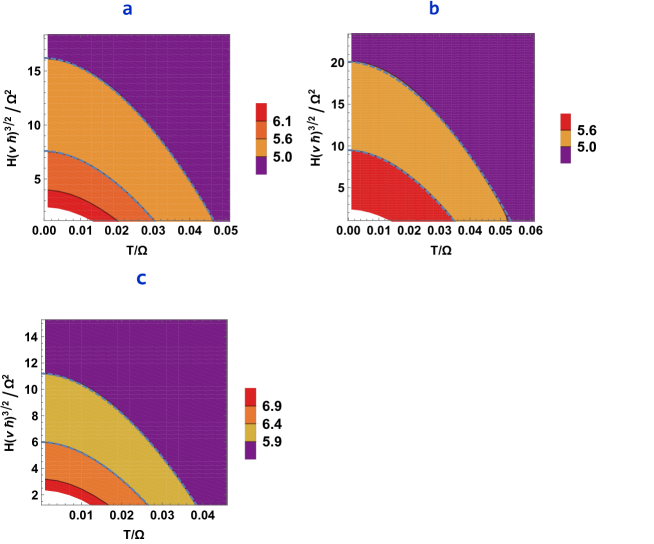
Figure 1: Upper critical field as a function on temperature for various adiabatic ratio $\gamma$ and electron-electron strength values $\lambda$ a) $\gamma=10$ b)  $\gamma=3$ c) $\gamma=1.$ Dash lines described by the universal interpolation formula (23) with reduced magnetic field $h^{\ast}=0.55$ parameter. Color scale marks $\lambda^{-1}$ magnitudes.

In Fig. 1 magnetic field is given in units of magnetic field $H_{u}=\Omega^{2}/\left(v\hbar\right)^{3/2}$ for three different values of the adiabaticity parameter $\gamma$ and the DSM superconductors electron velocity $v=10^{7}cm/\sec,$ typical to these materials. The temperature dependence $H_{c2}\left(T\right)$ is fitted very well by an interpolation formula,

$$H\left(T\right)=H\left(0\right)\left(1-\left(T/T_{c}\right)^{1/h^{\ast}}\right)\text{,}$$ (23)

for the universal value of the reduced magnetic field $h^{\ast}=0.55$ determining the exponent. Results of the theory demonstrates excellent agreement with temperature dependence of the upper critical magnetic field measured in DSM $TaP$ TaP , see Fig.2.

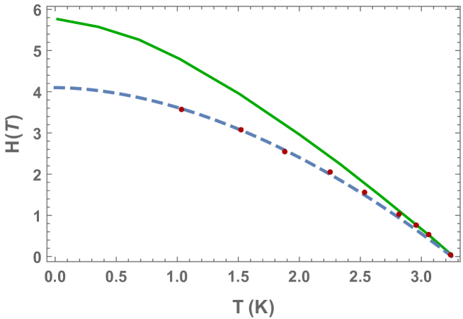
Figure 2: Upper Critical magnetic field $H_{c2}$ versus temperature for DSM $TaP$. The green curve marks result of the WHH theory for clean conventional superconductor. Red dots are the experimental data while the dash line is result of our theory.

In more general case when velocity in the $z$ axis direction (parallel to the magnetic field) $v_{z}$ is not zero, the upper critical field does not depends on $v_{z}$ since it renormalized the density of states and hence the electron-electron strength constant. The reduced magnetic field $h^{\ast}$ in this case coincides with that calculated for layered system (similar to conventional superconductors Bulaevsky ).

IV Conclusions

In this paper,the microscopic semi-classical theory of phonon mediated superconductivity in Dirac semimetals at magnetic fields was constructed in entire range of the temperature. Main results are presented in Figs. 1-2. Within the weak coupling approach, the retardation effects were explicitly taken into account by the dispersionless model of the electron - phonon coupling, Eq.(21). This is of importance since commonly used step function produce spurious oscillationRMP ; strongfield . The upper critical magnetic field $H_{c2}$ for graphene like Dirac semimetal was calculated for all temperatures in 2D and 3D Dirac superconductors. It is predicted that in Dirac semimetals the upper critical magnetic field $H_{c2}\left(T\right)$ is lower than predicted by the conventional Werthamer -Helfand -Hohenberg formula WHH derived for superconductors with parabolic dispersion relation. The reduced magnetic field ratio is universal (independent of the chemical potential, interaction strength etc.) and smaller than the Werthamer ratio $h^{\ast}=H_{c2}\left(0\right)/\left(-T\frac{dH_{c2}}{dT}\right)|_{T_{c}}$ for clean superconductors: $h^{\ast}=0.55$ for WSM, $h^{\ast}\left(0\right)=0.69$ for parabolic band. This explains the recent experiments on $Cd_{3}As_{2},ZrTe_{5}$ and especially on $TaP$ (see ref. CdAs , superWSM3D and TaP respectively). Going beyond semi - classical approximation is typically more complicated and has been contemplated in parabolic band materials India and recently in Weyl semimetalsstrongfield ; Manivnew .

Acknowledgements.

We are grateful to T. Maniv for valuable discussions. B. R. acknowledges MOST of ROC grant 107-2112-M-009-009-MY3, hospitality of Peking and Bar Ilan Universities. D.P. Li was supported by National Natural Science Foundation of China (Nos. 11274018 and 11674007).

References

• (1) Werthamer N.R. , Helfand E. , and Hohenberg P.C. , Phys. Rev. 147 (1966) 295 ; Helfand E. and Werthamer N. R. , Phys. Rev. Let. 13 (1964) 686.
• (2) Wang Z. , et al. Phys. Rev. B 85 (2012) 195320 ; Liu Z. K. , et al. Nat. Mater. 13 (2014) 677; Lv B. Q., et al. Nat. Phys. 11 (2015) 724;  Lv B. Q. , et al. Phys. Rev. X 5 (2015) 031013;Liu Z. K. , et al., Science 343 (2014) 864.
• (3) Liu H.-C. et al, Phys. Rev. B 93 (2016)144514.
• (4) Neupane M. , Xu S.-Y. ,Sankar R. , et al., Nat. Com. 5 (2014) 3786; Bachmann M. D. et al. Sci Adv. 24 (2017) 1602983, Zhou Y. H. , et al., PNAS 113 (2016) 2904.
• (5) Cao J. , et al, Nat. Comm. 6 (2015) 7779.
• (6) Xiao R. C. , et al. Phys. Rev. B 96 (2017) 075101.
• (7) Liu Y. , et al, Sci. Rep. 7 (2016) 44357.
• (8) Zhang J.-L. et al. Front. Phys., 7 (2012) 193.
• (9) Rosenstein B. , Shapiro B.Ya. , Li D. and Shapiro I . J. Phys. Cond. Mat. 27 (2015) 025701.
• (10) Das Sarma S. and Li Q. , Phys. Rev. B 88 (2013) 081404(R);Brydon P. M. R., Das Sarma S.,Hui H.-Y. and Sau J. D., Phys. Rev. B 90 (2014) 184512.
• (11) Fu L. and Berg E. , Phys. Rev. Lett. 105 (2010) 097001.
• (12) Li D. , Rosenstein B. , Shapiro B. Ya. ,and Shapiro I. , Phys. Rev. B 90 (2014) 054517.
• (13) Teknowijoyo S. et al, Phys. Rev. B 98 (2018) 024508.
• (14) Katayama S. ,Kobayashi A. , Suzumura Y. , J. Phys. Soc. Japan 75 (2006) 054705; Goerbig M. O. , Fuchs J. - N. , Montambaux G., Piéchon F. , Phys. Rev. B 78 (2008) 045415; Hirata M. et al, Nature Commun. 7 (2016) 12666.
• (15) Soluyanov A. A. , Gresch D. ,Wang Z. , Wu Q. , Troyer M. , Dai X. and Bernevig B. A. , Nature 527 (2015) 495.
• (16) Qi Y. et al., Nat. Comm. 7 (2016) 11038.
• (17) Rosenstein B. , Shapiro B. Ya. , Li D. , and Shapiro I. , Phys. Rev. B 97 (2018) 144510.
• (18) Song K. W. and Koshelev A. E. , Phys. Rev. B 95 (2017) 174503.
• (19) Li D. , Rosenstein B. , Shapiro B. Ya. and Shapiro I., Phys. Rev. B 96 (2017) 224517.
• (20) Zhou Y. et al. PNAS 113 (2016) 2904.
• (21) Wang Z, et al. Phys Rev B 85 (2012) 195320; Liu Z. K., et al. Science 343 (2014) 864; Xu S-Y, et al. Science 347 (2015) 294; Wang Z, Weng H, Wu Q, Dai X, Fang Z., Phys Rev B 88 (2013) 125427; Borisenko S, et al. Phys. Rev Lett 113 (2014) 027603; Liu Z. K, et al. Nat. Mater. 13 (2014) 677; Liang T, et al. Nat. Mater. 14 (2015) 280; He L.P., et al. Phys. Rev Lett 113 (2014) 246402; Jeon S. , et al. Nature Mat. 13 (2014) 851.
• (22) Li Y. , et al Quantum Materials 2 (2017) 66; B. Q. Lv et al Phys. Rev. X 5 (2015) 031013.
• (23) Gor’kov L.P. , Sov.Phys. JETP 10 (1960) 593 [Zh. Eksperim. i Teor. Fiz., 37 (1959) 833].
• (24) Bulaevsky L.N. , Sov. Phys. JETP,  38 (1974) 634 [Zh. Eksperim. i Teor. Fiz., 65 (1973) 1258].
• (25) Chandrasekhar B. S. , Appl. Phys. Lett. 1 (1962) 7 ; Clogston A. M. , Phys. Rev. Lett. 9 (1962) 266.
• (26) Li D. , Rosenstein B. , Shapiro B. Ya. , and Shapiro I. , Phys. Rev. B 95 (2017) 094513.
• (27) Wang Z. et al, Phys. Rev. B 85 (2012) 195320.
• (28) Abrikosov A. A. , Gor’kov L. P. , Dzyaloshinskii I. E. , Quantum field theoretical methods in statistical physics, (1965) Pergamon Press, New York.
• (29) Li D. , Rosenstein B. , Shapiro B. Ya. , and Shapiro I., Phys. Rev. B 95 (2017) 094513.
• (30) Rasolt M. and Tesanovic Z. , Rev. Mod. Phys., 64 (1992) 709; Maniv T. , Rom A. I. ,Vagner I. D. ,Wyder P. , Phys. Rev. B 46 (1992) 8360; Maniv T. , Zhuravlev V. ,Vagner I. ,Wyder P. , Rev. Mod. Phys., 73 (2001) 868.
• (31) Rajacopal A. K. ,Vasudevan R. , Phys. Lett. 20 (1966) 585; ibid 23 (1966) 539.
• (32) Gradshtein I.S. and Ryzhik I.M. , Table of Integrals, Series, and Products, Seventh Edition, (2007) Alan Jeffrey and Daniel Zwillinger (eds).
• (33) Zhuravlev V., Duan W. and Maniv T. EPL 120 27004.