Broad Wings around H$\alpha$ and H$\beta$ in the Two S-Type Symbiotic Stars Z Andromedae and AG Draconis

Abstract

Symbiotic stars often exhibit broad wings around Balmer emission lines, whose origin is still controversial. We present the high resolution spectra of the S type symbiotic stars Z Andromedae and AG Draconis obtained with the ESPaDOnS and the 3.6 m Canada France Hawaii Telescope to investigate the broad wings around H$\alpha$ and H$\beta$. When H$\alpha$ and H$\beta$ lines are overplotted in the Doppler space, it is noted that H$\alpha$ profiles are overall broader than H$\beta$ in these two objects. Adopting a Monte Carlo approach, we consider the formation of broad wings of H$\alpha$ and H$\beta$ through Raman scattering of far UV radiation around Ly$\beta$ and Ly$\gamma$ and Thomson scattering by free electrons. Raman scattering wings are simulated by choosing an H I region with a neutral hydrogen column density $N_{HI}$ and a covering factor $CF$. For Thomson wings, the ionized scattering region is assumed to cover fully the Balmer emission nebula and is characterized by the electron temperature $T_{e}$ and the electron column density $N_{e}$. Thomson wings of H$\alpha$ and H$\beta$ have the same width that is proportional to $T_{e}^{1/2}$. However, Raman wings of H$\alpha$ are overall three times wider than H$\beta$ counterparts, which is attributed to different cross section for Ly$\beta$ and Ly$\gamma$. Normalized to have the same peak values and presented in the Doppler factor space. H$\alpha$ wings of Z And and AG Dra are observed to be significantly wider than H$\beta$ counterpart, favoring the Raman scattering origin of broad Balmer wings.

1 Introduction

Symbiotic stars are wide binary systems of a hot white dwarf and a mass losing giant (e.g. Kenyon, 2009). They are important objects for studying the mass loss and mass transfer processes. Their UV-optical spectra are characterized by prominent emission lines with a large range of ionization encompassing C II and O VI. Symbiotic activities including outbursts and bipolar outflows are attributed to the gravitational capture of some fraction of slow stellar wind from the giant component by the hot white dwarf (e.g., Skopal, 2008; Mikołajewska, 2012).

According to IR spectra, symbiotic stars are classified into ‘S’ type and ‘D’ type. ‘D’ type symbiotic stars exhibit an IR excess indicative of the presence of a warm dust component with $T_{D}\sim 10^{3}{\rm\ K}$ (e.g. Angeloni et al., 2010), whereas no such features are found in the spectra of ‘S’ type symbiotics. The orbital properties also differ greatly between these two types of symbiotics. The orbital periods are found to be of order several hundred days for ‘S’ type symbiotics, implying that the binary separation is about several AU (e.g. Mikołajewska, 2012). However, the orbital periods of D type symbiotic stars are notoriously difficult to measure and only poorly known (e.g. Schmid, 1996, 2000).

Symbiotic stars show unique spectroscopic features at around 6825 Å and 7082 Å, which are formed through Raman scattering of far UV resonance doublet O VI $\lambda\lambda$1032 and 1038. Schmid (1989) proposed that an O VI$~{}\lambda$1032 photon is incident on a hydrogen atom in the ground state, which subsequently de-excites into $2s$ state emitting an optical photon at 6825 Å. The 7082 feature is formed in a similar way when O VI $\lambda$1038 photons are Raman scattered by neutral hydrogen atoms. The cross section for O VI is of order $10^{-22}{\rm\ cm^{2}}$ requiring the presence of a thick H I component in the vicinity of a hot emission nebula.

High resolution spectroscopy shows that most symbiotic stars exhibit broad wings around H$\alpha$, which often extend to several thousand ${\rm\ km\ s^{-1}}$ (e.g., Van Winckel et al., 1993; Ivison et al., 1994; Skopal, 2006; Selvelli & Bonifacio, 2000). Nussbaumer et al. (1989) proposed that Raman scattering by atomic hydrogen can give rise to broad wings around Balmer emission lines. Lee (2000) showed that the broad wings of many symbiotic stars are consistent with a profile proportional to $\Delta\lambda^{-2}$ that is expected of Raman scattering wings. Similar results for broad H$\alpha$ wings in a number of planetary nebulae and symbiotic stars were obtained by Arrieta & Torres-Peimbert (2003). These objects share the common property that a thick neutral component is present in the vicinity of a hot ionizing source.

Broad wings can also be formed through Thomson scattering, where emission line photons are scattered off of fast moving electrons to get broadened (e.g. Sekeráš & Skopal, 2012). In particular, Sekeráš & Skopal (2012) performed profile analyses of broad wings of O VI and He II emission lines and estimated the Thomson scattering optical depth and electron temperature of the symbiotic stars, AG Draconis, Z Andromedae and V1016 Cygni.

Z And is regarded as a prototypical symbiotic star with an M-type giant whose mass is $\sim 2{\rm\ M_{\odot}}$ (e.g. Mürset & Schmid, 1999). The mass of the white dwarf has been reported to be $0.75{\rm\ M_{\odot}}$. The orbital period is not accurately known and presumed to be in the range $759.0\pm 1.9$ days (e.g., Fekel et al., 2000). Having a K-type giant component, AG Dra is known to be a yellow symbiotic star (e.g. Mürset & Schmid, 1999). It has been reported that the masses of the white dwarf and the giant components of AG Dra are $1{\rm\ M_{\odot}}$ and $0.5{\rm\ M_{\odot}}$, respectively. The known binary orbital period of 550 days implies that the binary separation is $\sim 0.3{\rm\ AU}$ (e.g., Fekel et al., 2000).

In this paper, we present broad wings around H$\alpha$ and H$\beta$ from high resolution spectra of the ‘S’ type symbiotic stars Z And and AG Dra obtained with the ESPaDOnS and the 3.6 m Canada-France-Hawaii Telescope (CFHT). The observed wing profiles are compared to the theoretical model wings obtained with a Monte Carlo technique. We propose that Raman scattering is consistent with the two wing features whereas other wing formation mechanisms present difficulty in reconciling with the observation.

2 Spectroscopic Observation and Broad Balmer Wings

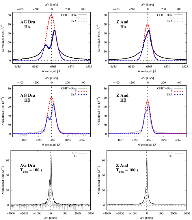
Figure 1: Spectra around H$\alpha$ and H$\beta$ obtained with the high resolution spectrograph ESPaDOnS and 3.6 m CFHT of the two ‘S’ type symbiotic stars AG Draconis (left panel) and Z And (right panel). The upper and lower horizontal axes show the Doppler factor from line center in units of ${\rm km\ s^{-1}}$ and the wavelength in units of $\rm\AA$, respectively. The top and middle panels show profiles of H$\alpha$ and H$\beta$ fitted with a single Gaussian emission component and an emission component with a Gaussian absorption, $G_{E}$ and $G_{EA}$. The black dashed lines are $x$ and $y$ axes. In the bottom panels, we overplot H$\alpha$ (black solid line) and H$\beta$ (grey solid line) in the Doppler factor space.

In Fig. 1, we show the spectra around H$\alpha$ and H$\beta$ emission lines of Z And and AG Dra obtained with the 3.6 m CFHT and ESPaDOnS on the nights of 2014 August 18 and September 6, respectively. The two symbiotic stars were observed in the “object only” spectroscopic mode with the spectral resolution of 81,000. The exposure time was 100 s. The standard procedure has been followed to reduce the observational data.

In the top and middle panels, the lower horizontal axis shows the wavelength $\lambda$ and the upper horizontal axis shows the Doppler factor $\Delta V$ defined as

$$\Delta V=\left({{\lambda-\lambda_{c}}\over{\lambda_{c}}}\right)c,$$ (1)

where $\lambda_{c}$ is the line center wavelength of either H$\alpha$ or H$\beta$ and $c$ is the speed of light. The weak underlying continuum is set to be a unit value and the profiles are normalized so that the two emission lines have the same peak value of 101. In Appendix A, we discuss the normalization of continuum fluxes and profiles in this work and conversion into physical units.

In the bottom panels, we overplot the H$\alpha$ and H$\beta$ profiles in the Doppler factor space in order for quantitative comparisons of the profiles. It is found that the H$\alpha$ profiles appear much broader than the H$\beta$ counterparts in these two symbiotic stars. Furthermore, H$\alpha$ wings are more conspicuous than H$\beta$ wings even when they are compared in the Doppler factor space. Hereafter, for ease of profile comparisons, we describe the profiles in the Doppler factor space.

The top and middle panels of Fig. 1 show our fit to H$\alpha$ and H$\beta$ using two functions, $G_{E}$ and $G_{EA}$ defined as follows

$$G_{E} = A_{E}\exp\left(-{{\Delta V}^{2}\over{2\sigma_{E}^{2}}}\right)$$

$$\tau_{A} = {\tau_{A0}\over{\sqrt{2\pi\sigma_{A}^{2}}}}\exp\left[-{({\Delta V-\Delta V_{A}})^{2}\over{2\sigma_{A}^{2}}}\right]$$

$$G_{EA} = G_{E}\exp(-\tau_{A}).$$

Here, $G_{E}$ represents a single Gaussian emission profile characterized by the peak $A_{E}$ and width $\sigma_{E}$, whereas $G_{A}$ represents an absorption component shifted by $\Delta V_{A}$ and characterized by the peak optical depth $\tau_{A0}$ and the width $\sigma_{A}$. The function $G_{EA}$ describes a single Gaussian emission superimposed by a single Gaussian absorption.

Table 2 shows the values of the parameters that characterize $G_{E}$ and $G_{A}$ for H$\alpha$ and H$\beta$ of the two objects. The peaks and widths of H$\alpha$ emission are larger than those of H$\beta$ emission, and also the same behavior is found for the H$\alpha$ and H$\beta$ absorption features. In the case of AG Dra, $\Delta V_{A}=-22{\rm\ km\ s^{-1}}$ for both H$\alpha$ and H$\beta$ and $\Delta V_{A}=-15{\rm\ km\ s^{-1}}$ for Z And. The effect of the absorption profiles of H$\alpha$ and H$\beta$ can be seen in the shoulder parts near $\Delta V\sim 100\rm\ km\ s^{-1}$. It should be noted that Balmer profiles of AG Dra and Z And differ significantly even in the core parts. However, in this work, we focus on the wing profiles of these two symbiotic stars.

Table 1: The parameters for core profiles of H$\alpha$ and H$\beta$ in Eq. (2)

Object	Line	$A_{E}$	$\sigma_{E}$	$\tau_{A0}$	$\sigma_{A}$	$\Delta V_{A}$
			${(\rm km\ s^{-1})}$		$({\rm km\ s^{-1})}$	${(\rm km\ s^{-1})}$
AG Dra	H$\alpha$	150	57	90	30	-22
AG Dra	H$\beta$	120	45	37	18	-22
Z And	H$\alpha$	120	44	20	27	-15
Z And	H$\beta$	110	35	10	13	-15

3 Wing Formation and the Monte Carlo Approach

3.1 Atomic Physics of Wing Formation

In this work, we consider two physical mechanisms that may be responsible for formation of broad wings around Balmer emission lines. One is Thomson scattering by free electrons and the other is Raman scattering by atomic hydrogen. In terms of the classical electron radius $r_{e}=e^{2}/(m_{e}c^{2})=2.82\times 10^{-13}{\rm\ cm}$, the Thomson scattering cross section is given as

$$\sigma_{Th}={8\pi\over 3}r_{e}^{2}=0.665\times 10^{-24}{\rm\ cm^{2}}.$$ (3)

The cross section $\sigma_{Th}$ is independent of the incident photon wavelength, which implies that line photons escape from the scattering region through spatial diffusion in a way completely analogous to a random walk process.

Thomson scattering is regarded as the low energy limit of Compton scattering, in which case there is fractional energy exchange $\Delta E/E\sim h\nu/(m_{e}c^{2})$. For a representative optical photon with $h\nu=2{\rm\ eV}$ it amounts to $\Delta E/E\sim 4\times 10^{-6}$. This is equivalent to a Doppler factor $\Delta V\sim 1.2{\rm\ km\ s^{-1}}$ or a redshift in the amount of $0.024{\rm\ \AA}$ for H$\alpha$ (e.g. Hummer & Mihalas, 1967).

Hummer (1962) presented the redistribution function in frequency space taking into account the non-coherency of Compton scattering. However, this effect provides almost negligible contribution to broad Balmer wings having widths in excess of $10^{3}{\rm\ km\ s^{-1}}$. In view of this fact, previous works by Laor (2006) and Kim et al. (2007) took into consideration only thermal motions of free electrons in order to to compute wing profiles of Thomson scattering.

In this work, we also consider only thermal motions of free electron in simulating Thomson scattering wings. In the rest frame of a free electron, Thomson scattering is described as an elastic scattering process where an incident photon changes its direction without any frequency shift. In the observer’s frame, the scattered photon acquires a Doppler shift corresponding to the electron velocity component along the difference in wavevectors of incident and scattered radiation.

We may expect that the width and strength of Thomson wings are mainly determined by the Thomson optical depth $\tau_{Th}=N_{e}\sigma_{Th}$ and the electron temperature $T_{e}$, where $N_{e}$ is the electron column density given by the product of the electron density $n_{e}$ and the characteristic length associated with the scattering region. The electron temperature representative of an emission nebula is $\sim 10^{4}{\rm\ K}$ (Osterbrock & Ferland, 2006), for which the electron thermal velocity is

$$v_{th}=\sqrt{kT_{e}\over m_{e}}=389\ T_{4}^{1/2}{\rm\ km\ s^{-1}},$$ (4)

where $T_{4}=T_{e}/10^{4}{\rm\ K}$. In terms of wavelength shift around H$\alpha$, this amounts to $\Delta\lambda_{th}=v_{th}\lambda_{H\alpha}/c=8.5{\rm\ \AA}$.

Broad wing features can develop around any spectral lines through Thomson scattering due to wavelength independence of the cross section. In constrast, Raman scattering by atomic hydrogen can produce broad wings around hydrogen emission lines except for Lyman lines, because the cross section is sharply peaked around hydrogen emission line centers. Raman scattering is a generic term describing an inelastic scattering process involving an incident photon and an electron bound to an atom or a molecule. In particular, far UV radiation near Ly$\beta$ and $Ly\gamma$ may be scattered by a hydrogen atom in the ground $1s$ state, which de-excites finally into the $2s$ state with the emission of an optical photon around H$\alpha$ and H$\beta$. The energy conservation requires the relation between wavelengths $\lambda_{i}$ and $\lambda_{o}$ of the incident and scattered radiation, respectively, given by

$$\lambda_{o}^{-1}=\lambda_{i}^{-1}-\lambda_{Ly\alpha}^{-1},$$ (5)

where $\lambda_{Ly\alpha}$ is the wavelength of Ly$\alpha$. A wavelength variation for the incident radiation $\Delta\lambda_{i}$ corresponds to a much broader wavelength range $\Delta\lambda_{o}$ shown as

$$\Delta\lambda_{o}=\left({\lambda_{o}\over\lambda_{i}}\right)^{2}\Delta\lambda_{i},$$ (6)

from which we recognize the broadening factors $\lambda_{o}/\lambda_{i}\simeq 6.4$ for H$\alpha$ and $\lambda_{o}/\lambda_{i}\simeq 5.0$ for H$\beta$.

The interaction of a photon and an electron is described by the second order perturbation theory, introduced in many textbooks on quantum mechanics including Sakurai (1967) and Bethe & Salpeter (1957). The cross section for Raman scattering is known as the Kramers-Heisenberg formula

$${d\sigma\over d\Omega} = r_{e}^{2}\left({\omega^{\prime}\over\omega}\right)\Bigg{|}{1\over m_{e}}\sum_{I}\left({({\bf p}\cdot\bm{\epsilon^{(\alpha^{\prime})}})_{BI}({\bf p}\cdot{\bm{\epsilon}^{(\alpha)}})_{IA}\over E_{I}-E_{A}-\hbar\omega}\right.$$ (7)

$$+ \left.{({\bf p}\cdot{\bm{\epsilon}^{(\alpha)}})_{BI}({\bf p}\cdot{\bm{\epsilon}^{(\alpha^{\prime})}})_{IA}\over E_{I}-E_{A}+\hbar\omega^{\prime}}\right)\Bigg{|}^{2},$$

where ${\bm{\epsilon}}^{(\alpha)}$ and ${\bm{\epsilon}}^{(\alpha^{\prime})}$ are polarization vectors associated with the incident and scattered photons, respectively (e.g. Saslow & Mills, 1969; Chang et al., 2015). Here, the initial state $A=1s$, the final state $B=2s$ and the intermediate state $I$ covers all bound $np$ states and continuum $n^{\prime}p$ states.

The Wigner-Eckart theorem asserts that one can decompose the matrix elements into the radial part and the angular part, where the angular part is averaged over unpolarized incident radiation and summed over all possible polarization states to yield the Rayleigh scattering phase function

$$<|{\bm{\epsilon}^{(\alpha)}}\cdot{\bm{\epsilon}^{(\alpha^{\prime})}}|>={8\pi\over 3}.$$ (8)

The matrix element associated with the momentum operator $p$ is simply related to the oscillator strength by

$$f_{nn^{\prime}}={2\over m_{e}\hbar\omega_{nn^{\prime}}}|p_{nn^{\prime}}|^{2},$$ (9)

and the Kramers-Heisenberg formula can be rearranged in terms of the oscillator strengths (e.g., Nussbaumer et al., 1989).

As far as the broad wings around H$\alpha$ are concerned, the wavelength range of interest lies in off-resonance regime sufficiently far from the Ly$\beta$ line center compared to the thermal width. Near Ly$\beta$, the cross section is dominantly contributed by the $3p$ term, in which case the cross section is excellently approximated by a Lorentzian function. According to Lee (2013),

$$\sigma^{\rm Ram}(\omega)\simeq{5\over 128}\sigma_{Th}\left({\omega_{32}\over\omega-\omega_{31}}\right)f_{13}f_{2s,3p},$$ (10)

where the oscillator strengths are

$$f_{13}=0.0791,\quad f_{2s,3p}=0.4349$$ (11)

(see e.g. Bethe & Salpeter, 1957).

In Fig. 2, we present the total cross section near Ly$\beta$ and Ly$\gamma$, which is characterized by the resonance behavior around line center. The figure also shows the branching ratio of Raman scattering into Balmer series, which is given as the ratio of the Raman cross section de-excited to $2s$ state divided by the total cross section. As Chang et al. (2015) pointed out, extremely broad Raman scattering wings of H$\alpha$ and H$\beta$ show asymmetry between redward and blueward. Also, a hydrogen atom in the excited $3p$ level de-excites into the level $2s$ with a probability of 0.12 and with the remaining probability of 0.88 it de-excites into the ground level.

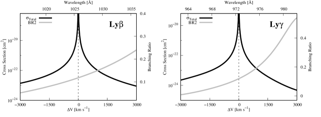
Figure 2: Total cross section (black solid lines) and Balmer branching ratios (grey solid lines) near Ly$\beta$ and Ly$\gamma$ computed using the Kramers-Heisenberg formula.

3.2 Scattering Geometries for Thomson and Raman Wings

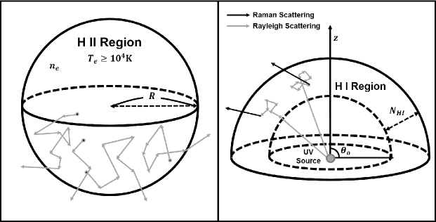
Figure 3: Scattering geometries of the Thomson scattering (left panel) and Raman scattering (right panel) adopted in this work. In the case of Thomson scattering, free electrons are distributed with a constant number density $n_{e}$ in a sphere with radius $R$. The sphere is characterized by the Thomson optical depth $\tau_{Th}=n_{e}\sigma_{Th}R$. H$\alpha$ line photons are assumed to be generated uniformly inside the sphere. In the case of Raman scattering, the scattering neutral region takes a form of a partial spherical shell with a half-opening angle $\theta_{o}$. The far UV emission source coincides with the center of the partial spherical shell.

The left panel of Fig. 3 illustrates schematically the Thomson scattering geometry considered in this work. We adopt a static H II region in the form of a sphere with radius $R$ and a uniform electron number density $n_{e}$, where hydrogen Balmer line photons are generated in a uniform fashion and Thomson scattered. We introduce the Thomson scattering optical depth $\tau_{Th}=n_{e}\sigma_{Th}R$ to characterize the H II region.

The parameter space considered in this work is described by the electron temperature $T_{e}\geq 10^{4}\,\rm K$ and the Thomson optical depth $\tau_{Th}\leq 0.1$. The Monte Carlo simulation for Thomson wings starts with a generation of a Balmer line photon in a random place inside the spherical H II region with an initial frequency chosen to be a Gaussian random deviate with the standard deviation of $\sigma_{v}=30{\rm\ km\ s^{-1}}$ in the Doppler space. It should be noted that this velocity is quite smaller than the electron thermal velocity $v_{th}\sim 390{\rm\ km\ s^{-1}}$ at $T_{e}=10^{4}\,\rm K$.

We show a scattering geometry of Raman scattering wings in the right panel of Fig. 3. Dumm et al. (1999) investigated an eclipsing symbiotic star SY Muscae to measure the H I column density as a function of binary orbital phase. They found that $N_{HI}$ varies from $10^{21}{\rm\ cm^{-2}}$ to $10^{25}{\rm\ cm^{-2}}$, where an extremely high column density of $10^{25}{\rm\ cm^{-2}}$ is limited to the orbital phase near $\phi_{orbit}=1$ with the giant companion in front of the white dwarf component. From this result, we may imagine that a neutral region with $N_{HI}\sim 10^{21}{\rm\ cm^{-2}}$ may surround the binary system quite extensively. In this work, the scattering neutral region is assumed to be a partial spherical shell with a half-opening angle $\theta_{o}$ which is converted to the covering factor $CF=(1-\cos\theta_{o})/2$.

We locate the far UV emission source at the center of the partial spherical shell. Treating as a point source, we consider flat and isotropic continuum around Lyman series. The partial spherical H I region is characterized by a neutral hydrogen column density $N_{HI}$ along the radial direction.

3.3 Monte Carlo Approach

We adopt a Monte Carlo technique to produce simulated wings around H$\alpha$ formed through Raman scattering and Thomson scattering. We generate a photon in the emission region with an initial wavevector ${\bf\hat{k}}$ and follow its path until escape from the scattering region. Thomson scattering is characterized by the scattering phase function given by

$$f(\mu)\propto 1+\mu^{2},$$ (12)

where $\mu=\cos\theta_{s}$ is the cosine of the angle $\theta_{s}$ between the incident and scattered wavevectors. The same phase function also describes Rayleigh and Raman scattering as long as the incident photon is off-resonant where the deviation from line center is sufficiently larger than the fine structure splitting (Stenflo, 1980).

A convenient formalism incorporating the polarization information is the density matrix approach, in which a Hermitian $2\times 2$ matrix [$\rho$] is associated with a given photon. The density matrix elements are easily interpreted in terms of the Stokes parameters $I,Q,U$ and $V$, where

$$I = \rho_{11}+\rho_{22}$$

$$Q = \rho_{11}-\rho_{22}$$

$$U = {1\over 2}{Re}[\rho_{12}]={1\over 2}{Re}[\rho_{21}]$$

$$V = {1\over 2}{Im}[\rho_{12}]=-{1\over 2}{Im}[\rho_{21}].$$ (13)

For a photon propagating in the direction ${\bf\hat{k}}=(\sin\theta\cos\phi,\sin\theta\sin\phi,\cos\theta)$, we may choose a set $\{|{\bm{\epsilon}_{1}}>,|{\bm{\epsilon}_{2}}>\}$ of basis vectors representing the polarization states, where

$$|{\bm{\epsilon}_{1}}> = (-\sin\phi,\cos\phi,0),$$

$$|{\bm{\epsilon}_{2}}> = (\cos\theta\cos\phi,\cos\theta\sin\phi,-\sin\theta).$$ (14)

The density matrix elements $\rho_{ij}^{\prime}$ associated with the scattered radiation with ${\bf\hat{k}}_{f}=(\sin\theta^{\prime}\cos\phi^{\prime},\sin\theta^{\prime}\sin\phi^{\prime},\cos\theta^{\prime})$ are related to those for the incident photon

$$\rho_{ij}^{\prime}=\sum_{kl}<{\bf\hat{e}}_{i}^{\prime}|{\bf\hat{e}}_{k}>\rho_{kl}<{\bf\hat{e}}_{j}^{\prime}|{\bf\hat{e}}_{l}>,$$ (15)

where $<{\bf\hat{e}}_{j}^{\prime}|{\bf\hat{e}}_{l}>$ is an inner product between the two polarization basis vectors $|{\bf\hat{e}}_{l}>$ and $|{\bf\hat{e}}_{i}^{\prime}>$ associated with the incident and scattered photons, respectively. A more detailed explanation can be found in (e.g. Lee et al., 1994; Ahn & Lee, 2015).

In the Monte Carlo simulations, each scattering optical depth $\tau$ traversed by a photon in the scattering region is given in a probabilistic way as

$$\tau=-\ln X,$$ (16)

where $X$ is a uniform random number between 0 and 1. This optical depth $\tau$ is inverted to a physical distance in order to locate the next scattering site. In the case of Thomson scattering, the physical distance $l_{Th}$ is given by

$$l_{\rm Th}={\tau\over{n_{e}\sigma_{Th}}}.$$ (17)

Using this value, we determine the next scattering position $\bm{r}_{s}$ by the relation

$$\bm{r}_{s}=\bm{r}_{i}+l_{\rm Th}\hat{\bm{k}},$$ (18)

where $\bm{r}_{i}$ is the position vector of the previous scattering site. If ${\bm{r}_{s}}$ is outside the ionized nebular region, the photon is considered to escape from the region to reach the observer. Otherwise, we iterate the process to find a new scattering position treating ${\bm{r}_{s}}$ as starting position.

In the case of transfer of a far UV photon near Ly$\beta$ and Ly$\gamma$, the photon under study may be Rayleigh scattered several times before it becomes an optical photon through Raman scattering. The H I region is assumed to be optically thin for optical photons near H$\alpha$ and H$\beta$ so that a Raman scattered photon directly escapes to reach the observer.

The physical distance $l_{\rm Ram}$ corresponding to a probabilistic scattering optical depth $\tau$,

$$l_{\rm Ram}={\tau\over{n_{HI}\sigma_{tot}}},$$ (19)

and the next scattering site is

$$\bm{r}_{s}=\bm{r}_{i}+l_{\rm Ram}\hat{\bm{k}}.$$ (20)

At the location of ${\bm{r}_{s}}$, we generate a new wavevector ${\bm{k}_{o}}$. Using another uniform random number $X^{\prime}$ and the Raman branching ratio $b$, decision is made for the scattering type. If it is Raman, then the photon is regarded as an optical photon, which directly escapes in the direction of ${\bm{k}_{o}}$. Otherwise, the scattering is Rayleigh and we determine the next scattering site by obtaining a revised $l_{\rm Ram}$.

In dealing with Rayleigh scattering, we fix the wavelength of a given photon because the thermal motion of an atomic hydrogen in H I region is negligible compared to the wing widths $>10^{3}\ \rm km\ s^{-1}$.

On the other hand, Thomson scattered photons suffer diffusion in frequency space with a step corresponding to the thermal motion of free electrons. The velocity of a free electron $\bm{v}_{th}$ is selected in a probabilistic way using Gaussian random deviates. The Thomson scattering is treated as elastic in the rest frame of the scatterer. Transforming to the observer’s frame, we obtain the relation between the wavelengths before and after scattering $\lambda_{i}$ and $\lambda_{f}$

$$\lambda_{f}=\left(1-{{\hat{\bm{k}_{f}}\cdot\bm{v}_{th}}\over c}\right)\left(1+{{\hat{\bm{k}}\cdot\bm{v}_{th}}\over c}\right)\lambda_{i}.$$ (21)

4 Simulated Broad Balmer Wing Profiles

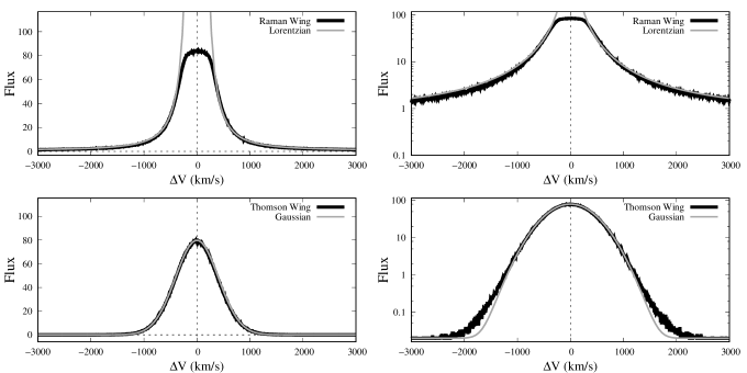
Figure 4: Black solid lines and grey solid lines show our Monte Carlo results and fitting functions for broad wings. The top panels and the bottom panels show Raman and Thomson scattering wings formed in scattering geometries illustrated in the right and left panels Fig 3, respectively. The fitting functions shown in grey solid lines are a Gaussian and a Lorentzian for Raman wings and Thomson wings, respectively.

In this section, we present broad wings obtained from our Monte Carlo calculations for Raman scattering with atomic hydrogen and Thomson scattering with free electrons. Two representative wing profiles are shown in Fig. 4, where the top and bottom panels are for Raman and Thomson wings, respectively. The black thick solid lines show our Monte Carlo result and grey thin solid lines are fitting functions.

In the left panels, the vertical scale is linear whereas the right panels are presented in logarithmic scale in order for easy comparisons with fitting functions. In the bottom right panel, the Thomson wings show excess at $|\Delta V|>1000{\rm\ km\ s^{-1}}$ compared to the fitting Gaussian function. Multiple Thomson scattering may result in deviation of the wing profile from a pure Gaussian, because Thomson scattering involves diffusion in frequency space as well as spatial diffusion (e.g., Kim et al., 2007).

The Raman wing feature is fitted with a Lorentzian function, because the Raman cross section near Ly$\beta$ is roughly approximated by a Lorentzian function due to the proximity of resonance (e.g., Lee, 2013). The Thomson wing profile is fitted with a Gaussian function because the free electron region is assumed to follow a Maxwell-Boltzmann distribution. As $\Delta V$ is increased, the Gaussian nature forces Thomson wings to decay much more rapidly than Raman wings.

4.1 Thomson Wings

Fig. 5 shows Thomson wings obtained from our Monte Carlo simulations for various values of the electron temperature $T_{e}$ and Thomson optical depth $\tau_{Th}$. The horizontal axis is the Doppler factor and the vertical axis is relative photon number represented in linear scale. In the Monte Carlo simulations, we collect only those photons Thomson scattered at least once ignoring emergent photons without being scattered at all.

In order to describe the Thomson wings in a quantitative way, we introduce a parameter ’TSF (Thomson scattered fraction)’ defined by

$${\rm TSF}(\Delta V)d(\Delta V)={N_{scat}(\Delta V)\over N_{init}}d(\Delta V).$$ (22)

Here, $N_{init}$ is the number of photons initially emitted from the uniform H II region and $N_{scat}(\Delta V)d(\Delta V)$ represents the number of collected photons having a Doppler factor in the interval $\Delta V$ and $\Delta V+d(\Delta V)$. For simplicity, we take $d(\Delta V)=100\,\rm km\,s^{-1}$. In Fig. 5, the vertical axis shows ’TSF’.

The left panels of Fig. 5 show Thomson wings for $T_{4}=1,2$ and $5$ with the Thomson optical depth fixed to $\tau_{Th}=0.1$. Because of small Thomson optical depth, the number of scattering averaged over all collected photons is slightly larger than unity. In this situation, the Thomson wings follow approximately a Maxwell-Boltzmann distribution with a width proportional to ${T_{e}}^{1/2}$. This is illustrated by the result that the total wing flux is almost constant while the width increases as $T_{e}$ increases.

The right panels show Thomson wings for various values of the Thomson optical depth $\tau_{Th}=0.01,0.05$ and $0.1$ at fixed $T_{4}=1$. For $\tau_{Th}<1$, the wing flux is roughly proportional to $\tau_{Th}$ while the profile width remains unchanged.

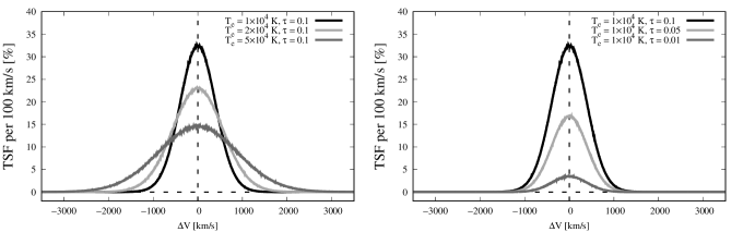
Figure 5: Thomson wing profiles obtained from our Monte Carlo simulations for various values of electron temperature $T_{e}$ and Thomson scattering optical depth $\tau_{Th}$. The left panel shows Thomson wings for three values of $T_{e}=1\times 10^{4},2\times 10^{4}$ and $3\times 10^{4}{\rm\ K}$ with the Thomson optical depth fixed to $\tau_{Th}=0.1$. The right panel shows Thomson wings for fixed $T_{e}=10^{4}{\rm\ K}$ and four values of $\tau_{Th}=0.01$, 0.05 and 0.1.

4.2 Raman Wings

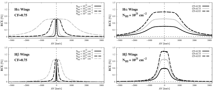
Figure 6: Monte Carlo simulated Raman wings around H$\alpha$ (top panels) and H$\beta$ (bottom panels) formed in a neutral partial spherical shell illustrated in the right panel of Fig. 3. The left panels show Raman wings for a fixed value of $CF=0.75$ varying the neutral hydrogen column density $N_{HI}$ in the range $10^{18}-10^{21}{\rm\ cm^{-2}}$. The right panels are Raman wings for various values of $\theta_{o}$ and a fixed $N_{HI}=10^{21}{\rm\ cm^{-2}}$.

Fig. 6 shows Raman wings near H$\alpha$ and H$\beta$ obtained with our Monte Carlo code, which simulates Raman wing formation in a neutral partial spherical shell illuminated by a flat continuum around Ly$\beta$ and Ly$\gamma$. For a flat incident continuum, the Raman wing profile is identified with the Raman conversion efficiency (RCE) per unit scattered wavelength $\lambda_{o}$, defined by

$${\rm RCE}(\lambda_{o})d\lambda_{o}={N_{Raman}\over N_{total}}d\lambda_{i}.$$ (23)

Here, $N_{total}$ is the number of incident photons from the flat and isotropic source per incident wavelength $\lambda_{i}$. The wavelength of Raman scattered radiation $\lambda_{o}$ is related to $\lambda_{i}$ by Eq. 5. We also denote by $N_{Raman}$ the number of Raman scattered photons collected over all lines of sight. In Fig. 6, the vertical axis shows ’RCE’ as a function of the Doppler factor in the observed frequency space. We consider various values of $N_{HI}=10^{18}-10^{21}\rm\,cm^{-2}$ and $CF=0.5-0.93$.

Quantitatively we obtain ${\rm RCE}\sim 0.01$ for H$\alpha$ and H$\beta$ wings, respectively. Quite unlike the case of Thomson wings, H$\alpha$ wings are much broader than those of H$\beta$, which is explained by overall larger cross section around Ly$\beta$ than Ly$\gamma$. As is shown in Fig. 6, the widths of Raman H$\alpha$ wings are almost three times larger than those of H$\beta$ in the Doppler space. The small Raman conversion efficiency is attributed to the smallness of the factor

$$A={d\lambda_{i}\over d\lambda_{o}}=\left({\lambda_{i}\over\lambda_{o}}\right)^{2},$$ (24)

which gives the ratio of the one-dimensional volumes of incident frequency space and Raman frequency space. Approximately the ratios are approximately $0.025$ and $0.04$ near H$\alpha$ and H$\beta$, respectively. A close look at Fig. 6 reveals higher ’RCE’ for H$\beta$ than H$\alpha$ near line center, where Raman scattering cross section is high. This is explained by the larger value of ’$A$’ factor for H$\beta$ than that for H$\alpha$.

Chang et al. (2015) showed that Raman wings around H$\alpha$, H$\beta$ and Pa$\alpha$ exhibit different widths and strengths when they are formed in a region with high column density $N_{HI}\geq 10^{22}\,\rm cm^{-2}$ due to significant differences in the cross section $\sigma^{Ram}(\omega)$ and branching channels. The widths of Raman wings are roughly proportional to $N_{HI}^{1/2}$ as Chang et al. (2015) showed. In the same work, the Raman conversion efficiency is saturated to remain flat near the line center, where the Raman scattering optical depth exceeds unity.

The right panels in Fig. 6 show our Monte Carlo results for three values of the covering factor ’$CF$’ at fixed $N_{HI}$. In the case of high $CF$, Rayleigh escaping far UV photons may reenter the scattering region to provide an additional contribution to the final ’RCE’. The effect of reentry is considered in this work, which results in nonlinear response of Raman wing flux as a function of ’$CF$’.

4.3 Comparison of Simulated Raman and Thomson Wings

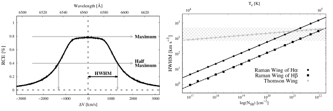
Figure 7: Half width at half maximum (HWHM) of Thomson and Raman wings computed with a Monte Carlo technique. HWHM of Thomson wings is presented with grey dots as a function of $T_{e}$ shown in the upper horizontal axis with a fixed $\tau_{Th}=0.1$. Data for Raman H$\alpha$ and H$\beta$ wings are shown by black circle and square marks, respectively, as a function of $N_{HI}$ corresponding to the lower horizontal axis.

In this subsection, we compare Raman wings around H$\alpha$ and H$\beta$ and Thomson wings produced in our Monte Carlo simulations. Fig. 7 shows the HWHM of Raman wings around H$\alpha$ (black dots) and H$\beta$ (black squares) obtained for various values of $N_{HI}=10^{17}-10^{22}\,\rm cm^{-2}$. The lower horizontal axis shows $N_{HI}$ in logarithmic scale. Note that the vertical scale is also logarithmic. We also plot the HWHM of Thomson wings with grey dots for various values of the electron temperature $T_{4}=1-10$. The upper horizontal axis represents $T_{e}$ in logarithmic scale. It should be noted that in the Doppler factor space Thomson wings of H$\alpha$ are identical with those of H$\beta$ due to the independence of Thomson cross section on wavelength.

The linear relations shown in logarithmic scales in Fig. 7 imply that the HWHMs of Raman and Thomson wings are related to $N_{HI}$ or $T_{e}$ by a power law. We provide the fitting relations as follows

$${\rm HWHM}_{\rm Raman\,H\alpha} = 418\ N_{20}^{0.49}\rm\ km\ s^{-1}$$

$${\rm HWHM}_{\rm Raman\,H\beta} = 135\ N_{20}^{0.49}\rm\ km\ s^{-1}$$

$${\rm HWHM}_{\rm Thomson\;\;\,} = 532\ T_{4}^{0.49}\rm\ km\ s^{-1},$$ (25)

where $N_{20}=N_{HI}/[10^{20}\ \rm cm^{-2}]$ is the H I column density divided by $10^{20}{\rm\ cm^{-2}}$.

The Raman wing widths are approximately proportional to $N_{HI}^{1/2}$, which is attributed to the fact that the total scattering cross sections around Lyman series are approximately proportional to $\Delta\lambda^{-2}$. On the other hand, the Thomson wing widths are proportional to $T_{e}^{1/2}$, which reflects the fact that the electron thermal speed $v_{th}\propto T_{e}^{1/2}$.

From Eq. (4.3), one may notice that the HWHMs of Raman H$\alpha$ wings are approximately three times as large as those for H$\beta$ . In the range of electron temperature $T_{4}=1-10$, the HWHM of Thomson wings lies in the narrow range of $1,080\pm 550{\rm\ km\ s^{-1}}$, reflecting the fact that the width of Thomson wings is mainly determined by the thermal electron speed $v_{th}$. Based on this result, it may be argued that Thomson scattering is inadequate to explain broad wings observed to exhibit $\rm{HWHM}<530{\rm\ km\ s^{-1}}$, noting that an ionized region is hardly colder than $10^{4}{\rm\ K}$ (e.g. Osterbrock & Ferland, 2006). The same argument can be made for wings that may exceed several $10^{3}{\rm\ km\ s^{-1}}$ often reported in the planetary nebula M2-9, for which Balick (1989) reported the presence of broad H$\alpha$ wings with a width $>10^{3}{\rm\ km\ s^{-1}}$.

For $N_{HI}=10^{20-21}{\rm\ cm^{-2}}$ and $T_{e}=10^{4-5}\ \rm K$, the widths of Raman H$\alpha$ wings and Thomson wings are comparable. In the case of Raman wings, H$\alpha$ wings are much broader than H$\beta$ counterparts by a factor of three, as stated earlier. The observational clear signature for Raman origin is the unambiguous disparity of the wing widths of H$\alpha$ and H$\beta$. However, observationally H$\beta$ is weaker than H$\alpha$ rendering H$\beta$ wings often poorly measured. In contrast to simulations, no unequivocal isolation of wing photons or scattered photons from the entire Balmer emission flux is apparent with the observed spectra, preventing one from measuring the HWHMs of the observed Balmer wings.

4.4 Comparison with the Observed Spectra of AG Dra and Z And

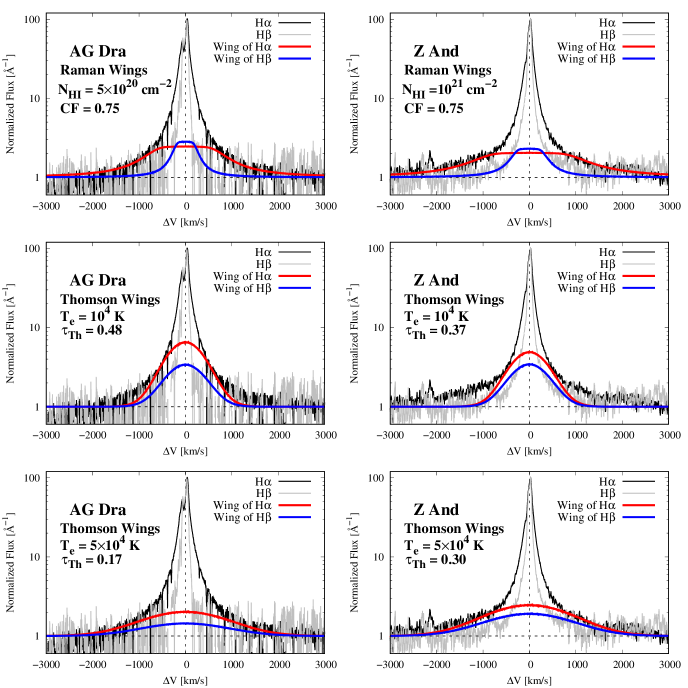
Figure 8: Comparison of our Monte Carlo wing profiles and the CFHT spectrum around H$\alpha$ and H$\beta$ of AG Dra (left panels) and Z And (right panels) obtained with CFHT. The horizontal axis is the Doppler factor in units of ${\rm km\ s^{-1}}$. The vertical scale is logarithmic normalized flux.

In this subsection, we compare our simulated wing profiles with the observed data in the Doppler factor space. H$\alpha$ and H$\beta$ profiles are normalized so that their peaks coincide with the numerical value of 101 and the underlying continuum has the value of 1. In Fig. 8, all the vertical axes are given in logarithmic scale.

The top two panels of Fig. 8 show our simulated Raman H$\alpha$ and H$\beta$ wings in red and blue lines, respectively, which provide our best fit to the CFHT spectra of AG Dra and Z And. The best fit profiles are selected by eye. The H I column densities adopted for the simulation are $N_{HI}=5\times 10^{20}\rm\ cm^{-2}$ and $10^{21}\rm\ cm^{-2}$ for AG Dra and Z And, respectively, with $CF=0.75$ for both objects. The contribution of the Raman wings to the observed H$\alpha$ and H$\beta$ is 15.5% and 14.7% for AG Dra and 16.3% and 12.2% for Z And.

We present a conversion between the relative flux scale in Fig. 1 and physical scale for a typical symbiotic star characterized by the white dwarf mass $M_{*}=0.6{\rm\ M_{\odot}}$ and a radius $R_{*}=0.01{\rm\ R_{\odot}}$ (Mürset et al., 1991). An accretion rate of $\dot{M}=10^{-7}{\rm\ M_{\odot}\ yr^{-1}}$ (Tomov & Tomova, 2002; Tomov et al., 2008) gives rise to the accretion luminosity

$$L_{acc}={GM_{*}\dot{M}\over R_{*}}\sim 200\ L_{\odot}.$$ (26)

According to Mürset et al. (1991) the luminosities of AG Dra and Z And are $10\,L_{\odot}$ and $600\,L_{\odot}$, respectively, whereas the temperature of the hot component is about $10^{5}{\rm\ K}$ for both the objects.

High ionization lines including O VI$\lambda\lambda$1032 and 1038 are common in many symbiotic stars indicating a hot ionizing source with $T_{h}\sim 10^{5}{\rm\ K}$ (Mürset et al., 1991; Birriel et al., 2000). The specific luminosity at around Ly$\beta$ from a black body with a temperature $T_{h}=1.5\times 10^{5}{\rm\ K}$ and luminosity $L_{acc}$ is

$$L_{\lambda}^{acc}\sim 8\times 10^{33}{\rm\ erg\ s^{-1}\ \AA^{-1}}.$$ (27)

The distances to AG Dra and Z And are poorly known and, for example, according to Tomov & Tomova (2002) and Tomov et al. (2008) they are 1.7 kpc for AG Dra and 1.1 kpc for Z And, respectively. In terms of the distance $D$, the flux density $F_{\lambda}^{acc}$ near Ly$\beta$ associated with the accretion specific luminosity in Eq. (27) is

$$F_{\lambda}^{acc}\sim 8.4\times 10^{-10}\left({D\over 1{\rm\ kpc}}\right)^{-2}{\rm\ erg\ cm^{-2}\ s^{-1}\ \AA^{-1}}.$$ (28)

In order to simulate the Raman wings around H$\alpha$ and H$\beta$ shown in the top panels of Fig. 8, continuum photons around Ly$\beta$ and Ly$\gamma$ are generated in the far UV emission source in Fig 3. In our simulation, we consider the incident continuum flux ($ICF_{Ly\beta}$) near Ly$\beta$ that is locally flat. The incident continuum flux is measured in unit of $\rm\AA^{-1}$ for which the physical conversion of the unit value of $ICF_{Ly\beta}=1{\rm\ \AA^{-1}}$ is discussed in Appendix B.

For the Raman wings of H$\alpha$ in Fig. 8, we find $ICF_{Ly\beta}=3.3\,\rm\AA^{-1}$ and $4.5\,\rm\AA^{-1}$ for AG Dra and Z And, respectively. If the H$\alpha$ line flux is $2\times 10^{-10}{\rm\ erg\ cm^{-2}\ s^{-1}}$, then these values are converted into $2.7\times 10^{-10}$ and $3.4\times 10^{-10}\ {\rm\ erg\ cm^{-2}\ s^{-1}\ \AA^{-1}}$ for AG Dra and Z And, respectively.

A similar procedure is taken for $ICF_{Ly\gamma}$ near Ly$\gamma$ for Raman wings around H$\beta$. In the simulations, we use $ICF_{Ly\gamma}=7.4\,\rm\AA^{-1}$ and $5.4\,\rm\AA^{-1}$ for AG Dra and Z And, respectively, which are transformed to $1.3\times 10^{-11}$ and $2.0\times 10^{-11}\ {\rm\ erg\ cm^{-2}\ s^{-1}\ \AA^{-1}}$, respectively. In Appendix B, the conversion of $ICF$ from our parametrization into physical units is discussed.

The middle and bottom panels Fig. 8 show Thomson wings simulated with two different values of $T_{e}=10^{4}{\rm\ K}$ and $T_{e}=5\times 10^{4}{\rm\ K}$ for comparisons with the observed data. In each panel, the Thomson H$\alpha$ profile is stronger than Thomson H$\beta$ counterpart, simply because we injected more H$\alpha$ photons than H$\beta$ photons. We compute the total number flux $TF_{H\alpha}$ of H$\alpha$ defined by

$$TF_{H\alpha}=\int_{\lambda(\Delta V=-500\,{\rm km/s})}^{\lambda(\Delta V=+500\,{\rm km/s})}NF_{H\alpha}(\lambda)d\lambda,$$ (29)

where $NF_{H\alpha}(\lambda)$ is the observed flux normalized to have the peak value of 101. In a similar way, $TF_{H\beta}$ is computed to yield the ratio of $TF_{H\alpha}/TF_{H\beta}=2.0$ and 1.6 for AG Dra and Z And, respectively.

These observed ratios are used to show Thomson H$\alpha$ and H$\beta$ wings in Fig. 8. In the middle panels ($T_{e}=10^{4}{\rm\ K}$), the Thomson optical depths are $\tau_{Th}=0.48$ and 0.37 for AG Dra and Z And. In the bottom panels ($T_{e}=5\times 10^{4}{\rm\ K}$), smaller values of $\tau_{Th}=0.17$ and 0.30 are used for AG Dra and Z And, respectively.

In the middle panel, the near wing parts $|\Delta V|<500{\rm\ km\ s^{-1}}$ are well fit whereas the quality of fit becomes poor in the far wing parts. An opposite behavior is seen in the bottom panel, where good fit is obtained in the far wing parts. It should be noted that the electron temperature $T_{e}=5\times 10^{4}{\rm\ K}$ is significantly higher than the values considered in the work of Sekeráš & Skopal (2012) who analyzed the Thomson wing profiles of O VI and He II emission lines.

5 Conclusion and Discussion

In this article, we used a Monte Carlo technique to produce broad wings around H$\alpha$ and H$\beta$. The adopted physical mechanisms include Thomson scattering of H$\alpha$ and H$\beta$ by free electrons and Raman scattering of Ly$\beta$ and Ly$\gamma$ by atomic hydrogen. In the case of Thomson wings, the wing profiles are well-approximated by a Gaussian function whose width is mainly determined by the temperature of the free electron region. The Thomson scattering optical depth determines the resultant Thomson wing flux.

On the other hand, Raman wing profiles follow the Lorentzian function, which also describes the cross section. In the case of Raman wings, the wing flux is mainly affected by the H I column density and the covering factor of the neutral region. The cross section near Ly$\beta$ is much larger than that near Ly$\gamma$, which leads to Raman H$\alpha$ wings much stronger than H$\beta$ counterpart. When Balmer lines are overplotted in the Doppler factor space, Raman H$\alpha$ wings are expected to appear stronger and broader than H$\beta$ wings.

We also presented high resolution spectra of the two S type symbiotic stars AG Dra and Z And obtained with the CFHT in 2014 in order to make quantitative comparisons with simulated Thomson and Raman wings. The observational data and simulated data were shown in logarithmic scale, from which we notice that Raman wings provide better fit than Thomson wings.

Sekeráš & Skopal (2012) presented a convincing argument that the broad wings around O VI and He II lines are formed through Thomson scattering. It may be that Balmer emission lines are formed in a more extended region than O VI and He II, having higher ionization potential than H I. In this case, it is expected that the fraction of Thomson scattered flux is much smaller for Balmer lines than for O VI and He II.

Considering the difficulty of explaining far wings with $\Delta V>10^{3}{\rm\ km\ s^{-1}}$ through Thomson scattering, it remains as an interesting possibility that near wing parts are significantly contributed by Thomson scattering whereas Raman scattering is the main contributor to the far wing parts. This possibility may imply complicated polarization behavior in the wing parts due to different scattering geometries for Thomson and Raman processes.

Broad wings can also be formed from a hot tenuous wind around the compact component with a high speed (e.g., Skopal, 2006). Because the flux ratio of H$\alpha$ and H$\beta$ in the fast wind will be given by the recombination rate, it is expected that the flux ratio in the wing part will be similar to that in the emission core part. This strongly implies that H$\alpha$ and H$\beta$ will show similar profiles in the Doppler factor space. In consideration of this, the disparity of wing widths in H$\alpha$ and H$\beta$ may indicate substantial contribution of Raman scattering to the Balmer wing formation.

Balmer wings formed through scattering are expected to develop significant linear polarization, implying that spectropolarimetry will shed much light on the physical origin. According to Kim et al. (2007), Thomson wings may exhibit a complicated polarization structure because multiply scattered photons tend to contribute more to the far wing parts than to the near wing parts. Kim et al. (2007) proposed that far wings are less strongly polarized than near wing regions.

In the case of Raman scattering, wings may also be strongly polarized depending on the scattering geometry and the location of far UV emission source. Yoo et al. (2002) investigated linear polarization and profiles of Raman scattered H$\alpha$ profiles. They proposed that the degree of linear polarization may increase as $\Delta V$ where single scattering dominates. Ikeda et al. (2004) carried out spectropolarimetry of AG Dra and Z And to propose that the polarization behavior of Raman O VI$\lambda$ 6825 is similar to that of H$\alpha$ wings lending support to the Raman scattering origin. However, their analysis of H$\alpha$ was limited to a relatively narrow region $|\Delta V|<500{\rm\ km\ s^{-1}}$, which is insufficient to rule out the formation through Thomson scattering.

Broad H$\alpha$ wings are also found in young planetary nebulae including IC5117 and IC4997 (e.g Lee & Hyung, 2000; Arrieta & Torres-Peimbert, 2002). Van de Steene et al. (2000) also reported that some post-AGB stars show broad H$\alpha$ wings. The operation of Raman scattering by atomic hydrogen is also known for far UV He II lines near H I Lyman series in symbiotic stars and a few planetary nebulae including NGC 7027, NGC 6790, IC 5117 and NGC 6302 (e.g. Kang et al., 2009; Lee et al., 2006; Péquignot et al., 1997; Groves et al., 2002). Raman scattered He II features are formed in the blue wing parts of Balmer emission lines. Raman scattering cross section of He II $\lambda$1025 is $\sigma\sim 7.2\times 10^{21}{\rm\ cm^{2}}$, from which a broad scattered feature is formed at 6545 Å. The planetary nebulae with Raman He II are known to exhibit broad H$\alpha$ wings, which may be regarded as circumstantial evidence of contribution to Balmer wings from Raman scattering.

Appendix A Normalization of CFHT data

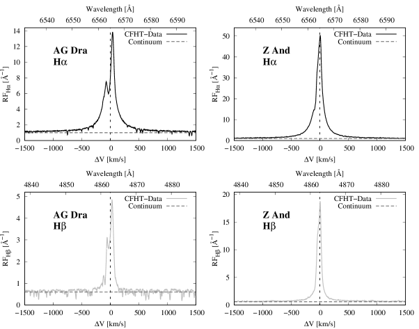
Figure 9: Comparison of our Monte Carlo wing profiles and the CFHT spectra around H$\alpha$ and H$\beta$ of AG Dra (left panels) and Z And (right panels) obtained with CFHT. The horizontal axises are the wavelength in units of $\rm\AA$ and the Doppler factor from line center in units of ${\rm km\ s^{-1}}$. The vertical axis is the relative flux.

Table 2: Parameters for the observed profiles of H$\alpha$ and H$\beta$ in Fig 9

Object	Line	$PV$	$CL$	$EW$
AG Dra	H$\alpha$	13.82 $\rm\AA^{-1}$	1.000 $\rm\AA^{-1}$	106.7 Å
AG Dra	H$\beta$	4.839 $\rm\AA^{-1}$	0.600 $\rm\AA^{-1}$	47.15 Å
Z And	H$\alpha$	50.44 $\rm\AA^{-1}$	1.000 $\rm\AA^{-1}$	238.8 Å
Z And	H$\beta$	18.77 $\rm\AA^{-1}$	0.600 $\rm\AA^{-1}$	88.70 Å

In Fig. 9, we show the spectra of AG Dra and Z And obtained with the CFHT. The spectra not being flux calibrated, the vertical axis shows the relative flux ($RF$) in an arbitrary scale per Å. In turn, Table 2 shows the measured values of the peak value ($PV$), continuum level ($CL$) and equivalent width ($EW$) for the H$\alpha$ and H$\beta$ emission lines. Transformation of the relative flux into a physical unit can be facilitated once the total line flux of an emission line is fixed. For example, Tomov & Tomova (2002) reported the total line flux of H$\alpha$ $F_{H\alpha}=2\times 10^{-10}{\rm\ erg\,cm^{-2}\,s^{-1}}$ for AG Dra and a similar value was also reported for Z And by Tomov et al. (2008). In this case, the unit relative flux ($RF=1{\rm\ \AA^{-1}}$) in the spectra of Fig. 9 corresponds to

$$RF=1{\rm\ \AA^{-1}}\,\iff{F_{H\alpha}\over EW}\left({CL\over 1{\rm\ \AA^{-1}}}\right)=2\times 10^{-12}\left({100\ {\rm\AA}\over EW}\right)\left({CL\over 1{\rm\ \AA^{-1}}}\right){\rm\ erg\,cm^{-2}\,s^{-1}\,\AA^{-1}}.$$ (A1)

Also it should be noted that the equivalent width $(EW)$ is independent of the scale.

In Figs. 1 and 8, the normalized flux ($NF$) was introduced for profile comparisons of H$\alpha$ and H$\beta$, where the normalized flux $(NF)$ is related to $RF$ by the following relation

$$NF=(RF-CL)\ \left[{{100{\rm\ \AA^{-1}}}\over{PV-CL}}\right]+(1{\rm\ \AA^{-1}}).$$ (A2)

With this relation, the normalized flux has the peak value to be 101 ${\rm\AA^{-1}}$ of $NF$ for both H$\alpha$ and H$\beta$. Because $PV$ and $CL$ of H$\alpha$ differ from those of H$\beta$, different conversion into a physical unit is applied for $NF_{H\alpha}$ around H$\alpha$ and $NF_{H\beta}$ around H$\beta$.

Around H$\alpha$, the unit value $NF_{H\alpha}=1{\rm\ \AA^{-1}}$ of the normalized flux corresponds to

$$NF_{H\alpha}=1{\rm\ \AA^{-1}}\,\iff\left({F_{H\alpha}\over EW}\right)\ \left({CL\over 1{\rm\ \AA^{-1}}}\right)\ \left({PV-CL\over 100{\rm\ \AA^{-1}}}\right),$$ (A3)

where $PV,CL$ and $EW$ are measured values for H$\alpha$. With the fiducial value of $F_{H\alpha}=2\times 10^{-10}{\rm\ erg\ s^{-1}\ cm^{-2}}$, we have

$$NF_{H\alpha}=1{\rm\ \AA^{-1}}\,\iff 2\times 10^{-12}\left[{PV-CL\over 100{\rm\ \AA^{-1}}}\right]\left[{CL\over 1{\rm\ \AA^{-1}}}\right]\left[{100{\rm\ \AA}\over EW}\right]{\rm\ erg\,cm^{-2}\,s^{-1}\,\AA^{-1}}.$$ (A4)

The ratios $F_{H\alpha}/F_{H\beta}$ measured from our CFHT spectra are 3.77 and 4.49 for AG Dra and Z And, respectively. Using these mesaured ratios, the normalized flux $NF_{H\beta}$ around H$\beta$ is converted into

$$NF_{H\beta}=1{\rm\ \AA^{-1}}\,\iff{F_{H\beta}\over EW}\ {CL\over 1{\rm\ \AA^{-1}}}\ {PV-CL\over 100{\rm\ \AA^{-1}}}.$$ (A5)

Adopting the ratio $F_{H\alpha}/F_{H\beta}$, $NF$ in unit of ${\rm\ \AA^{-1}}$ in the simulation is converted to

$$NF_{H\beta}=1{\rm\ \AA^{-1}}\,\iff 2\times 10^{-12}\left[{F_{H\beta}\over F_{H\alpha}}\right]\left[{PV-CL\over 100{\rm\ \AA^{-1}}}\right]\left[{CL\over 1{\rm\ \AA^{-1}}}\right]\left[{100{\rm\ \AA}\over EW}\right]{\rm\ erg\,cm^{-2}\,s^{-1}\,\AA^{-1}}.$$ (A6)

Appendix B Converting from UV radiation to Raman scattering wing

In our simulations, far UV continuum photons around Ly$\beta$ and Ly$\gamma$ are generated and subsequently injected into neutral region to investigate the formation of Raman wings around H$\alpha$ and H$\beta$. Because the incident far UV continuum level in the simulation is also presented in unit of ${\rm\AA^{-1}}$ just like the normalized flux around H$\alpha$ and H$\beta$ discussed above, we discuss the conversion of the continuum level into the physical unit of ${\rm erg\ cm^{-2}\ s^{-1}\ \AA^{-1}}$.

Raman scattering relocates a far UV continuum photon into a Balmer wing region. The relocation involves the factor $(\lambda_{o}/\lambda_{i})^{2}\simeq 40$ between the wavelength space near Ly$\beta$ and that near H$\alpha$. That is, a continuum interval of size $d\lambda_{i}$ around Ly$\beta$ is “Raman-transformed” onto an interval around H$\alpha$ of size $d\lambda_{o}\simeq 40\ d\lambda_{i}$. In addition, another factor of $\lambda_{o}/\lambda_{i}$ should be considered because an H$\alpha$ photon is less energetic than a Ly$\beta$ photon by the same factor.

Therefore, the incident continuum flux ($ICF$) around Ly$\beta$ in unit of ${\rm\AA^{-1}}$ (i.e., $ICF_{Ly\beta}=1\ \rm\AA^{-1}$) is amplified by the factor $(\lambda_{o}/\lambda_{i})^{3}\simeq 250$ compared to $NF_{H\alpha}$ in Eq. A4. In the case of $F_{H\alpha}=2\times 10^{-10}{\rm\ erg\ s^{-1}\ cm^{-2}}$, the unit value of $ICF$ around Ly$\beta$ is converted into a physical unit of ${\rm\ erg\,cm^{-2}\,s^{-1}\,\AA^{-1}}$ as follows

$$ICF_{Ly\beta}=1{\rm\ \AA^{-1}}\iff 5\times 10^{-10}\left[{PV-CL\over 100{\rm\ \AA^{-1}}}\right]\left[{CL\over 1{\rm\ \AA^{-1}}}\right]\left[{100{\rm\ \AA}\over EW}\right]{\rm\ erg\,cm^{-2}\,s^{-1}\,\AA^{-1}}.$$ (B1)

Here, $PV$, $CL$ and $EW$ are the parameters of the H$\alpha$ line presented in Table 2.

Similarly the factor of $(4850/972)^{3}\sim 100$ is involved in the wavelength space near Ly$\gamma$ and that around H$\beta$. Adopting Eq. (A6), $ICF_{Ly\gamma}$ is

$$ICF_{Ly\gamma}=1{\rm\ \AA^{-1}}\iff 2\times 10^{-10}\left[{PV-CL\over 100{\rm\ \AA^{-1}}}\right]\left[{CL\over 1{\rm\ \AA^{-1}}}\right]\left[{100{\rm\ \AA}\over EW}\right]{\rm\ erg\,cm^{-2}\,s^{-1}\,\AA^{-1}}.$$ (B2)

The Raman wings around H$\alpha$ shown in Fig. 8 are generated with the incident continuum flux $ICF_{Ly\beta}=3.3\,\rm\AA^{-1}$ and $4.5\,\rm\AA^{-1}$ for AG Dra and Z And, respectively. With the normalization of $F_{H\alpha}=2\times 10^{-10}{\rm\ erg\ cm^{-2}\ s^{-1}}$, the corresponding far UV continuum around Ly$\beta$ would be $2.7\times 10^{-10}{\rm\ erg\ cm^{-2}\ s^{-1}\ \AA^{-1}}$ and $3.4\times 10^{-10}{\rm\ erg\ cm^{-2}\ s^{-1}\ \AA^{-1}}$ for AG Dra and Z And, respectively. Similarly for the Raman wings around H$\beta$ shown in Fig. 8, $ICF_{Ly\gamma}=7.4\,\rm\AA^{-1}$ and $5.4\,\rm\AA^{-1}$ for AG Dra and Z And, respectively, which are converted into $1.3\times 10^{-11}\ {\rm\ erg\ cm^{-2}\ s^{-1}\ \AA^{-1}}$ and $2.0\times 10^{-11}\ {\rm\ erg\ cm^{-2}\ s^{-1}\ \AA^{-1}}$.

References

- Ahn & Lee (2015) Ahn, S.-H. & Lee, H.-W., 2015, JKAS, 48, 195
- Akras et al. (2017) Akras, S., Gonçalves, D. R., Ramos-Larios, G., 2017, MNRAS, 465, 1289
- Angeloni et al. (2010) Angeloni, R., Contini, M., Ciroi, S., Rafanelli, P., 2010, MNRAS, 402, 2075
- Arrieta & Torres-Peimbert (2002) Arrieta, A., Torres-Peimbert, S, 2002, RMxAC, 12, 154
- Arrieta & Torres-Peimbert (2003) Arrieta, A., Torres-Peimbert, S, 2003, ApJS, 147, 97
- Balick (1989) Balick, B., 1989, AJ, 97, 476
- Bethe & Salpeter (1957) Bethe, H. A. & Salpeter, E. E., 1957, Quantum Mechanics of One and Two Electron Atoms (New York: Academic Press)
- Birriel et al. (2000) Birriel, J., Espey, B. R., Schulte-Ladbeck, R. E., 2000, ApJ, 545, 1020
- Chang et al. (2015) Chang, S.-J. Heo, J.-E., Di Mille, F., Angeloni, R., Palma, T., Lee, H.-W., 2015, ApJ, 814, 98
- Dumm et al. (1999) Dumm, T., Schmutz, W., Schild, H., Nussnaumer, H., 1999, A&A, 349, 169
- Fekel et al. (2000) Fekel, F. C., Hinkle, K. H., Joyce, R. R., Skrutskie, M. F., 2000, AJ, 120, 3255
- Groves et al. (2002) Groves, B, Dopita, M. A., Williams, R. E., Hua, C.-T., 2002, PASA, 19, 425G
- Hummer (1962) Hummer, D. G., 1962, MNRAS, 125, 21
- Hummer & Mihalas (1967) Hummer, D. G., Mihalas, D., 1967, ApJ, 150L, 57
- Ikeda et al. (2004) Ikeda, Y., Akitaya, H., Matsuda, K., Homma, K., Seki, M., 2004, ApJ, 604, L357
- Ivison et al. (1994) Ivison, R. J., Bode, M. F., Meaburn, J., 1994, A&AS, 103, 2011
- Kenyon (2009) Kenyon, S. J., 2009, The Symbiotic Stars(Reading, UK: Cambridge University Press)
- Kang et al. (2009) Kang, E.-H., Lee, B.-C., Lee, H.-W., 2009, ApJ, 695, 542K
- Kim et al. (2007) Kim, H. J., Lee, H.-W. & Kang, S., 2007, MNRAS, 374, 187
- Laor (2006) Laor, A., 2006, ApJ, 643, 112
- Lee et al. (1994) Lee, H.-W., Blandford, R. D., Western, L., 1994, MNRAS, 267, 303
- Lee (2000) Lee, H.-W., 2000, ApJL, 541, L25
- Lee & Hyung (2000) Lee, H.-W., Hyung, S., 2000, ApJL, 530, L49
- Lee et al. (2006) Lee, H.-W., Jung, Y.-C., Song, I.-O., Ahn, S.-H., 2006, ApJ, 636, L1045
- Lee (2013) Lee, H.-W., 2013, ApJ, 772, 123
- Mikołajewska (2012) Mikołajewska, J., 2012, Baltic Astronomy, 21, 5
- Mürset & Schmid (1999) Mürset, U., Schmid, H., M., 1999, A&AS, 137, 473
- Mürset et al. (1991) Mürset, U., Nussbaumer, H., Schmid, H., M., Vogel, M., 1991, A&A, 248, 458
- Nussbaumer et al. (1989) Nussbaumer, H., Schmid, H. M., Vogel, M., 1989, A&A, 211, L27
- Péquignot et al. (1997) Péquignot, D., Baluteau, J.-P., Morisset, C., Boisson, C., 1997, A&A, 323, 217
- Osterbrock & Ferland (2006) Osterbrock, D. E., Ferland, G. J., 2006, Astrophysics of gaseous nebulae and active galactic nuclei (Reading CA: University Science Books)
- Sakurai (1967) Sakurai, J. J., 1967, Advanced Quantum Mechanics (Reading, MA: Addison-Wesley)
- Saslow & Mills (1969) Saslow, W. M., & Mills, D. L., 1969, PhRv, 187, 1025
- Schmid (1989) Schmid, H. M., 1989, A&A, 211, L31
- Schmid (1996) Schild, H, Schmid, H. M., 1996, A&A, 310, 211
- Schmid (2000) Schmid, H. M., Corradi, R., Krautter, J., Schild, H, 2000, A&A, 355, 261
- Sekeráš & Skopal (2012) Sekeráš, M., Skopal, A., 2012, MNRAS, 427, 979
- Selvelli & Bonifacio (2000) Selvelli, P. L., Bonifacio, P., 2000, A&A, 364, 1
- Skopal (2006) Skopal, A., 2006, A&A, 457, 1003
- Skopal (2008) Skopal, A., 2008, JAVSO, 36, 9
- Stenflo (1980) Stenflo, J. O., 1980, A&A, 84, 68
- Tomov & Tomova (2002) Tomov, N. A., Tomova, M. T., 2002, A&A, 388, 202
- Tomov et al. (2008) Tomov, N. A., Tomova, M. T., Bisikalo, D. V., 2008, MNRAS, 389, 829
- Yoo et al. (2002) Yoo, J. J., Bak, J.-Y., Lee, H.-W., 2002, MNRAS, 336, 467
- Van Winckel et al. (1993) Van Winckel, H., Duerbeck, H. W., Schwarz, H. E., 1993, A&AS, 102, 401
- Van de Steene et al. (2000) van de Steene, G. C., Wood, P. R., van Hoof, P. A. M., 2000, ASPC, 199, 191