Least Squares Finite Element Methods for Sea Ice Dynamics

Abstract

A first-order system least squares formulation for the sea-ice dynamics is presented. In addition to the displacement field, the stress tensor is used as a variable. As finite element spaces, standard conforming piecewise polynomials for the displacement approximation are combined with Raviart-Thomas elements for the rows in the stress tensor. Computational results for a test problem illustrate the least-squares approach.

1 Introduction

Ice and snow covered surfaces reflect more than half of the solar radiation they are recieving and play therefore a major role in climate modelling. Each year, Antarctic sea ice extent reaches its maximum (17-20 million square kilometers) in September and its minimum (3-4 million square kilometers) in February. These important oscillations make the current predictive models of Antarctic sea ice require an accurate knowledge and understanding of the processes. Developing computational sea-ice modelling based on observed and measured data to study and predict the break-up and fracture evolution of sea-ice during the Antarctic spring was one of main scientific aims of the Winter 2017 cruise (Voyage 25) of the S.A. Agulhas II. This was funded by DST/NRF and took place from 28 June to 13 July 2017.

Sea ice is a complex material which is formed by the freezing of sea water. Since the ice stress is a source in the other equations of the climate models, its approximation plays an important role in the simulations of the ice. They can be computed from the velocity in a post-processing step, but the loss of accuracy due to the reconstruction step can lead to non-physical solutions. An alternative approach consists in the use of variational formulations involving the stress ${\boldsymbol{\sigma}}\in H({\rm div},\Omega)$ as an independent variable. Appropriate finite element spaces based on a triangulation $\mathcal{T}$ are the $H({\rm div},\Omega)$-conforming spaces, e.g. the Raviart-Thomas Space.

2 Problem Formulation

As most sea ice dynamic models currently used, our model is based on the viscous-plastic formulation introduced by Hibler [5]. There, sea ice is modeled by its velocity ${\bf{u}}$, the ice concentration $A$ and the average ice height $H$ over a domain $\Omega$. The model consists in a momentum equation for the velocity ${\bf{u}}$ and the balance laws for ice concentration $A$ and the average ice height $H$. Neglegting the thermodynamical effects, i.e. the source terms in these balance laws, the model can be written as

$$\begin{split}\rho_{ice}H\frac{\partial{\bf{u}}}{\partial t}+{\bf F}({\bf{u}})-{\rm div}\ {{\boldsymbol{\sigma}}({\bf{u}},A,H)}&=0,\\ \frac{\partial A}{\partial t}+{\rm div}({\bf{u}}A)&=0,\quad\frac{\partial H}{\partial t}+{\rm div}({\bf{u}}H)=0\ ,\end{split}$$ (1)

where the force term involving the ice, air and water densities $\rho_{ice}$,$\rho_{a}$ and $\rho_{o}$, the air and water drag coefficients $C_{a}$ and $C_{o}$, the coriolis parameter $f_{c}$, the radial unit vector ${\bf e}_{r}$ and the velocity fields ${\bf{v}}_{o}$ and ${\bf{v}}_{a}$ of ocean and atmospheric flow is given by

$${\bf F}({\bf{v}})=f_{c}{\bf e}_{r}\times({\bf{v}}-{\bf{v}}_{o})-\underbrace{\rho_{a}C_{a}\|{\bf{v}}_{a}\|_{2}{\bf{v}}_{a}}_{=:\mbox{\boldmath$\tau$}_{a}}-\underbrace{\rho_{o}C_{o}\|{\bf{v}}_{o}-{\bf{v}}\|_{2}({\bf{v}}_{o}-{\bf{v}})}_{=:\mbox{\boldmath$\tau$}_{o}({\bf{v}})}$$ (2)

and the stress-strain relation involving the ice strength parameter $P^{\star}$ and the ice concentration parameter $C$ is given by

$$\begin{split}&{\boldsymbol{\sigma}}=\frac{P}{2}\left(\frac{{{\rm dev}\ \mbox{\boldmath$\varepsilon$}({\bf{u}})}+2{{\rm tr}\ \mbox{\boldmath$\varepsilon$}({\bf{u}})}{\bf I}}{\Delta({\bf{u}})}-{\bf I}\right)\quad\text{with }P=P^{\star}He^{-C(1-A)}\\ &\text{and }\ \Delta({\bf{u}})=\sqrt{{\rm dev}\ \mbox{\boldmath$\varepsilon$}({\bf{u}}):{\rm dev}\ \mbox{\boldmath$\varepsilon$}({\bf{u}})+{4}{\rm tr}(\mbox{\boldmath$\varepsilon$}({\bf{u}}))^{2}+\Delta_{min}^{2}}\end{split}$$ (3)

where $\Delta_{min}=2\cdot 10^{-9}\ s^{-1}$ is a limitation for $\Delta({\bf{u}})$. In [7], the authors propose a variational formulation where $({\bf{u}},{\bf p})$ with ${\bf p}=(A,H)$ is sought in $\left(H^{1}_{0}(\Omega)\right)^{2}\times\left(L^{2}(\Omega)\right)^{2}$ such that

$$\begin{split}\left(\rho_{ice}H\frac{\partial{\bf{u}}}{\partial t},{\bf{v}}\right)+({\bf F}({\bf{u}}),{\bf{v}})+({\boldsymbol{\sigma}}({\bf{u}},H,A),\nabla{\bf{v}})&=0,\\ \left(\frac{\partial{\bf p}}{\partial t}+\nabla{\bf p}\cdot{\bf{u}}+{\rm div}({\bf{u}}){\bf p},{\bf q}\right)&=0\end{split}$$ (4)

holds for all $({\bf{v}},{\bf q})\in\left(H^{1}_{0}(\Omega)\right)^{2}\times\left(L^{2}(\Omega)\right)^{2}$. The constraints $H\geq 0$ and $A\in[0,1]$ are embedded in the trial-spaces and are realized by a projection of the solution.

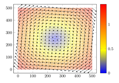
Figure 1: Wind field at $t=0$ (left) and Ocean current (right)

3 A Least-Squares Method

The Least-Squares Mehtod (see [2]) consists in minimizing the $L^{2}$-residuals in the partial differential equations. Therefore, we insert define a new variable ${\boldsymbol{\sigma}}$ for the stress and consider the stress-strain relationship (3) as and additional equation in order to obtain the following first order system for $({\boldsymbol{\sigma}},{\bf{u}},A,H)$:

$$\rho_{ice}H\frac{\partial{\bf{u}}}{\partial t}+{\bf F}({\bf{u}})-{\rm div}\ {{\boldsymbol{\sigma}}} =0 \frac{\partial A}{\partial t}+{\rm div}({\bf{v}}A) =0$$

$$\frac{P(A,H)}{2}\left(\frac{{\rm dev}\ \mbox{\boldmath$\varepsilon$}({\bf{u}})}{\Delta({\bf{u}})}+\frac{2{\rm tr}\ \mbox{\boldmath$\varepsilon$}({\bf{u}})}{\Delta({\bf{u}})}{\bf I}-{\bf I}\right) ={\boldsymbol{\sigma}} \frac{\partial H}{\partial t}+{\rm div}({\bf{v}}H) =0\$$

The least-squares functionals then reads

$${\cal F}({\boldsymbol{\sigma}},{\bf{u}},H)={\cal F}_{m}({\boldsymbol{\sigma}},{\bf{u}},A,H)+{\cal F}_{c}({\boldsymbol{\sigma}},{\bf{u}},A,H)+{\cal F}_{e}({\boldsymbol{\sigma}},{\bf{u}},A,H)$$ (5)

with

$$\begin{split}{\cal F}_{m}({\boldsymbol{\sigma}},{\bf{u}},A,H)&=\left\|\rho_{ice}H\frac{\partial{\bf{u}}}{\partial t}+{\bf F}({\bf{u}})-{\rm div}\ {{\boldsymbol{\sigma}}}\right\|_{0}^{2},\\ \quad{\cal F}_{e}({\boldsymbol{\sigma}},{\bf{u}},A,H)&=\left\|\frac{\partial H}{\partial t}+{\rm div}({\bf{u}}H)\right\|_{0}^{2}+\left\|\frac{\partial A}{\partial t}+{\rm div}({\bf{u}}A)\right\|_{0}^{2},\\ {\cal F}_{c}({\boldsymbol{\sigma}},{\bf{u}},A,H)&=\left\|{\boldsymbol{\sigma}}-\frac{P(A,H)}{2}\left(\frac{{\rm dev}\ \mbox{\boldmath$\varepsilon$}({\bf{u}})}{\Delta({\bf{u}})}+\frac{{\rm tr}\ \mbox{\boldmath$\varepsilon$}({\bf{u}})}{\Delta({\bf{u}})}{\bf I}-{\bf I}\right)\right\|_{0}^{2}\ .\\ \end{split}$$

The time discretization can be realised using a $\theta$-scheme and decoupling the advection equations from the rest of the system such that for each time step $n+1$, the linear functional

$$\begin{split}{\cal G}^{n+1}(A^{n+1},H^{n+1};{\bf{u}}^{n},H^{n},A^{n})=&\left\|\frac{H^{n+1}-H^{n}}{t^{\Delta}}+{\rm div}({\bf{u}}^{n}H^{n+1})\right\|_{0}^{2}\\ &+\left\|\frac{A^{n+1}-A^{n}}{t^{\Delta}}+{\rm div}({\bf{u}}^{n}A^{n+1})\right\|_{0}^{2}\end{split}$$ (6)

is first minimized over all $(A^{n+1},H^{n+1})\in\left(L^{2}(\Omega)\right)^{2}$, and then the functional

$$\begin{split}{\cal F}^{n+1}({\boldsymbol{\sigma}}^{n+1}&,{\bf{u}}^{n+1};{\boldsymbol{\sigma}}^{n},{\bf{u}}^{n},A^{n+1},H^{n+1})\\ &=\left\|\rho_{ice}H^{n+1}\frac{{\bf{u}}^{n+1}-u^{n}}{t^{\Delta}}+{\bf F}({\bf{u}}^{n+\theta})-{\rm div}\ {\boldsymbol{\sigma}}^{n+\theta}\right\|_{0}^{2}\\ &\ +{\cal F}_{c}({\boldsymbol{\sigma}}^{n+1},{\bf{u}}^{n+1};A^{n+1},H^{n+1})\end{split}$$ (7)

with the time discretized variables

$${\bf{u}}^{n+\theta}=\theta{\bf{u}}^{n+1}+(1-\theta){\bf{u}}^{n}$$

and

$${\boldsymbol{\sigma}}^{n+\theta}=\theta{\boldsymbol{\sigma}}^{n+1}+(1-\theta){\boldsymbol{\sigma}}^{n}\ ,$$

is minimized over all $({\boldsymbol{\sigma}}^{n+1},{\bf{u}}^{n+1})\in\left(H_{\text{div}}(\Omega)\right)^{2}\times\left(H^{1}_{\Gamma_{D}}(\Omega)\right)^{2}$. For the spacial discretization, a conforming subspace ${\bf W}_{h}$ of $\left(H_{\text{div}}(\Omega)\right)^{2}\times\left(H^{1}_{\Gamma_{D}}(\Omega)\right)^{2}\times\left(L^{2}(\Omega)\right)^{2}$. Therefore, a triangulation $\mathcal{T}_{h}$ of the domain $\Omega$ is considered. In this work, we choose ${\bf W}_{h}=(RT_{1}^{2}(\mathcal{T}_{h})\times\mathcal{P}_{2}^{2}(\mathcal{T}_{h}))\times\mathcal{P}_{1}^{2}(\mathcal{T}_{h}))$ in order to have appropriate convergence properties.

For the minimization of the nonlinear Functional $\mathcal{{\cal F}}^{n+1}$ in each time step, the Least-Squares Functional is linearized around a given approximation $({\boldsymbol{\sigma}}^{k},{\bf{u}}^{k},A^{k},H^{k})$ and the minimization is then carried out iteratively solving a sequence of linearized least squares problems. Additionaly the Least-Squares Functional is minimized subejct to the linear inequality constraints $A\in[0,1]$ and $H\geq 0$, that leads to a constraint optimization problem that we solved with an active set strategy. Since the variables $A$ and $H$ are now decoupled from ${\bf{u}}$ and ${\boldsymbol{\sigma}}$, we can define the stress-strain relation ship by

$$\begin{split}\mathcal{C}({\bf{u}};A,H):={\boldsymbol{\sigma}}({\bf{u}};A,H)=\frac{P(A,H)}{2}\left(\frac{{{\rm dev}\ \mbox{\boldmath$\varepsilon$}({\bf{u}})}+2{{\rm tr}\ \mbox{\boldmath$\varepsilon$}({\bf{u}})}{\bf I}}{\Delta({\bf{u}})}-{\bf I}\right)\end{split}$$ (8)

The Gateaux derivative of $\mathcal{C}({\bf{u}};A,H)$ in direction ${\bf{v}}$ is denoted by $\mathcal{C}({\bf{u}};A,H)[{\bf{v}}]$ and given by

$$\begin{split}\mathcal{J_{C}}({\bf{u}};A,H)[{\bf{v}}]=\frac{P(A,H)}{2}\left(\frac{{{\rm dev}\ \mbox{\boldmath$\varepsilon$}({\bf{v}})}+2{{\rm tr}\ \mbox{\boldmath$\varepsilon$}({\bf{v}})}{\bf I}}{\Delta({\bf{u}})}+\mathcal{J}_{\Delta^{-1}}({\bf{u}})[{\bf{v}}]\left({{\rm dev}\ \mbox{\boldmath$\varepsilon$}({\bf{u}})}+2{{\rm tr}\ \mbox{\boldmath$\varepsilon$}({\bf{u}})}{\bf I}\right)\right)\end{split}$$ (9)

with $\mathcal{J}_{\Delta^{-1}}({\bf{u}})[{\bf{v}}]=-\Delta({\bf{u}})^{-3}\left({\rm dev}\ \mbox{\boldmath$\varepsilon$}({\bf{u}}):{\rm dev}\ \mbox{\boldmath$\varepsilon$}({\bf{v}})+{4}{\rm tr}(\mbox{\boldmath$\varepsilon$}({\bf{u}})){\rm tr}(\mbox{\boldmath$\varepsilon$}({\bf{v}}))\right)$.

The first variation of the minimization of $\mathcal{{\cal F}}^{n+1}$ is then given by

$$\begin{split}\mathcal{B}({\boldsymbol{\sigma}}^{n+1},&{\bf{u}}^{n+1};\mbox{\boldmath$\tau$},{\bf{v}};{\boldsymbol{\sigma}}^{n},{\bf{u}}^{n},A^{n+1},H^{n+1})=\left.\frac{\partial{\cal F}^{n+1}({\boldsymbol{\sigma}}^{n+1}+\tau\mbox{\boldmath$\tau$},{\bf{u}}^{n+1}+\tau{\bf{v}};{\boldsymbol{\sigma}}^{n},{\bf{u}}^{n},A^{n},H^{n})}{\partial\tau}\right|_{\tau=0}\\ =&\left.\frac{\partial}{\partial\tau}\left({\boldsymbol{\sigma}}^{n+1}+\tau\mbox{\boldmath$\tau$}-\mathcal{C}({\bf{u}}^{n+1}+\tau{\bf{v}};A^{n+1},H^{n+1}),{\boldsymbol{\sigma}}^{n+1}+\tau\mbox{\boldmath$\tau$}-\mathcal{C}({\bf{u}}^{n+1}+\tau{\bf{v}};A^{n+1},H^{n+1})\right)\right|_{\tau=0}\\ &+2\left(\rho_{ice}H^{n+1}\frac{{\bf{u}}^{n+1}-u^{n}}{t^{\Delta}}-{\rm div}(\theta{\boldsymbol{\sigma}}^{n+1}+(1-\theta){\boldsymbol{\sigma}}^{n}),\rho_{ice}H^{n+1}\frac{\theta{\bf{v}}}{t^{\Delta}}-{\rm div}(\theta\mbox{\boldmath$\tau$})\right)\\ &+\left.\frac{\partial}{\partial\tau}\left({\bf F}(\theta{\bf{u}}^{n+1}+\theta\tau{\bf{v}}+(1-\theta){\bf{u}}^{n}),{\bf F}(\theta{\bf{u}}^{n+1}+\theta\tau{\bf{v}}+(1-\theta){\bf{u}}^{n})\right)\right|_{\tau=0}\\ +&2\left.\frac{\partial}{\partial\tau}\left(\rho_{ice}H^{n+1}\frac{{\bf{u}}^{n+1}+\tau{\bf{v}}-u^{n}}{t^{\Delta}}-{\rm div}(\theta{\boldsymbol{\sigma}}^{n+1}+\theta\tau\mbox{\boldmath$\tau$}+(1-\theta){\boldsymbol{\sigma}}^{n}),{\bf F}(\theta{\bf{u}}^{n+1}+\theta\tau{\bf{v}}+(1-\theta){\bf{u}}^{n})\right)\right|_{\tau=0}\\ =&2\left({\boldsymbol{\sigma}}^{n+1}-\mathcal{C}({\bf{u}}^{n+1};A^{n+1},H^{n+1}),\mbox{\boldmath$\tau$}-J_{\mathcal{C}}({\bf{u}}^{n+1};A^{n+1},H^{n+1})[{\bf{v}}]\right)\\ &+2\left(\rho_{ice}H^{n+1}\frac{{\bf{u}}^{n+1}-u^{n}}{t^{\Delta}}+{\bf F}({\bf{u}}^{n+\theta})-{\rm div}\ {\boldsymbol{\sigma}}^{n+\theta},\rho_{ice}H^{n+1}\frac{{\bf{v}}}{t^{\Delta}}+J_{{\bf F}}({\bf{u}}^{n+\theta})[\theta{\bf{v}}]-\theta{\rm div}\ \mbox{\boldmath$\tau$}\right)\ .\end{split}$$

Setting this first variation to zero leads to a necessary condition such that the Gauß-Newton Methods in each time step consits in setting iterativly $({\boldsymbol{\sigma}}^{n+1,k+1},{\bf{u}}^{n+1,k+1})=({\boldsymbol{\sigma}}^{n+1,k},{\bf{u}}^{n+1,k})+(\delta{\boldsymbol{\sigma}},\delta{\bf{u}})$ where $(\delta{\boldsymbol{\sigma}},\delta{\bf{u}})\in(RT_{0}^{2}(\mathcal{T}_{h})\times\mathcal{P}_{1}^{2}(\mathcal{T}_{h}))$ is the solution of

$$\begin{split}\mathcal{B}(&{\boldsymbol{\sigma}}^{n+1,k},{\bf{u}}^{n+1,k};\mbox{\boldmath$\tau$},{\bf{v}};{\boldsymbol{\sigma}}^{n},{\bf{u}}^{n},A^{n+1},H^{n+1})=\left(\delta{\boldsymbol{\sigma}}-J_{\mathcal{C}}({\bf{u}}^{n+1,k};A^{n+1},H^{n+1})[\delta{\bf{u}}],\mbox{\boldmath$\tau$}-J_{\mathcal{C}}({\bf{u}}^{n+1,k};A^{n+1},H^{n+1})[{\bf{v}}]\right)\\ &+\left(\rho_{ice}H^{n+1}\frac{\delta{\bf{u}}}{t^{\Delta}}+J_{{\bf F}}(\theta{\bf{u}}^{n+1,k}+(1-\theta){\bf{u}}^{n})[\theta\delta{\bf{u}}]-\theta{\rm div}\ \delta{\boldsymbol{\sigma}},\rho_{ice}H^{n+1}\frac{{\bf{v}}}{t^{\Delta}}+J_{{\bf F}}(\theta{\bf{u}}^{n+1,k}+(1-\theta){\bf{u}}^{n})[\theta{\bf{v}}]-\theta{\rm div}\ \mbox{\boldmath$\tau$}\right)\\ &\text{for all $(\mbox{\boldmath$\tau$},{\boldsymbol{\sigma}})\in(RT_{0}^{2}(\mathcal{T}_{h})\times\mathcal{P}_{1}^{2}(\mathcal{T}_{h}))$.}\end{split}$$

4 Test Case

In order to investigate the approximation properties of the Least-Squares method, we consider the same test case as in [7], involving a quadratic domain (see also [6]) and simulating the sea ice dynamics for $T=8$ days. Since the Least-Squares Method approximates all the residuals of the partial differential equation simultaneously, we scale the domain to the unit square $\Omega=[0,1]^{2}$. Since the wind field is a cyclone from the midpoint of the computational domain to the edge followed by an anticyclone diagonally passing from the edge to the midpoint, we define the time $t^{m}=t-4$ measured in days with respect to the time when the wind forcing alternates from cyclonic to anticyclonic. Further, let $\tilde{\bf{x}}(t)={\bf{x}}-{\bf{x}}^{m}(t)$ denote the position with respect to the center of the cyclone ${\bf{x}}^{m}(t)=x^{m}(t)({\bf e}_{1}+{\bf e}_{2})$ with $x^{m}(t)=0.1(9-|t^{m}|)$. Then, the prescribed wind field is given by

$${\bf{v}}_{a}=10{v_{a}^{m}}\left(1-\frac{2}{e^{t^{m}}e^{8-|t^{m}|}+1}\right)e^{-\frac{\|\tilde{\bf{x}}(t)\|_{2}}{10}}{\bf R}\left(\frac{17}{40}\pi+\frac{t^{m}}{40|t^{m}|}\pi\right)\tilde{\bf{x}}$$ (10)

$$\quad\text{with }{\bf R}(\vartheta)={\begin{pmatrix}\cos\vartheta&-\sin\vartheta\\ \sin\vartheta&\cos\vartheta\end{pmatrix}}\ ,$$ (11)

and a maximal wind velocity $v_{a}^{m}$, while the circular steady ocean current is

$${\bf{v}}_{o}=v_{o}^{m}\begin{pmatrix}2y-1\\ 1-2x\end{pmatrix}$$ (12)

with a maximal ocean velocity $v_{o}^{m}$. Finally, the initial conditions are given by zero velocity, constant ice concentration $A=1$ and $H^{0}(x,y)=0.3+0.005(\sin(250x)+\sin(250y))$. All simulations are executed with Fenics, using the inherent Newton solver. The velocity results at $t=2,4,6,8$ days are shown in the figure 3. Further intervestigations are needed, in particular regarding the ellipticity of the Least-Squares Functional, the possibility of considering domain with curved boundaries (see [1]) and the relation to others standard or mixed methods (as in [4]).

Parameter	Value
maximal ocean velocity $v_{o}^{m}$	$0.01$ ms${}^{-}1$
maximal ocean velocity $v_{a}^{m}$	$15$ ms${}^{-}1$
sea ice density $\rho_{ice}$	$900$ kg m${}^{-}3$
air density $\rho_{a}$	$1.3$ kg m${}^{-}3$
water density $\rho_{o}$	$1026$ kg m${}^{-}3$
air drag coefficient $C_{a}$	$1.2\cdot 10^{-3}$
water $C_{o}$	$5.5\cdot 10^{-3}$
coriolis parameter $f_{c}$	$1.46\cdot 10^{-4}$ s${}^{-}1$
ice strength parameter $P^{\star}$	$27.5\cdot 10^{3}$ Nm${}^{-}2$
ice concentration parameter $C$	20

Figure 2: Parameter used in the simulation

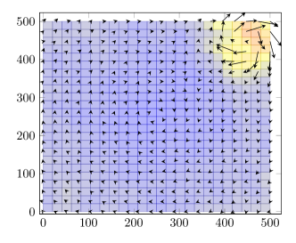
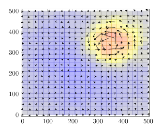
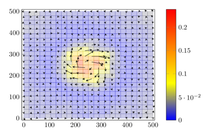
Figure 3: Sea-ice velocity at $t=2,4,6,8$.

References

- [1] F. Bertrand, S. Münzenmaier, and G. Starke First-order System Least Squares on Curved Boundaries: Higher-order Raviart–Thomas Elements. SIAM J. Numer. Anal. (2014) 52, 3165-3180.
- [2] P. Bochev and M. Gunzburger, Least-Squares Finite Element Methods, Springer, New York, 2009.
- [3] D. Boffi, F. Brezzi, and M. Fortin, Mixed Finite Element Methods and Applications, Springer, Heidelberg, 2013.
- [4] J. Brandts, Y. Chen and J. Yang A note on least-squares mixed finite elements in relation to standard and mixed finite elements. IMA J. Numer. Anal. (2006) 26: 779-789.
- [5] W.D. Hibler A dynamic thermodynamic sea ice model. J. Phys. Oceanogr (1979) 566 9(4):815-846.
- [6] E.C. Hunke Viscous-plastic sea ice dynamics with the EVP model: linearization isues. J. Comp. Phys. (2001) 170:18-38.
- [7] C. Mehlmann und T. Richter, A modified global Newton solver for viscous-plastic sea ice models, Ocean Modeling, Vol. 116, p.96:107, 2017.