The Inverse Grating Problem: Efficient Design of Anomalous Flexural Wave Reflectors and Refractors

Abstract

We present an extensive formulation of the inverse grating problem for flexural waves, in which the energy of each diffracted mode is selected and the grating configuration is then obtained by solving a linear system of equations. The grating is designed as a lineal periodic repetition of a unit cell comprising a cluster of resonators attached at points whose physical properties are directly derived by inversion of a given matrix. Although both active and passive attachments can be required in the most general case, it is possible to find configurations with only passive, i.e. damped, solutions. This inverse design approach presents an alternative to the design of metasurfaces for flexural waves overcoming the limitations of gradient phase metasurfaces, which require a continuous variation of the surface’s impedance. When the grating is designed in such a way that all the energy is channeled to a single diffracted mode, it behaves as an anomalous refractor or reflector. The negative refractor is analyzed in depth, and it is shown that with only three scatterers per unit cell is it possible to build such a device with unitary efficiency.

I Introduction

The fundamental property of gratings to redirect wave energy into multiple diffracted modes, transmitted and reflected, follows from simple considerations of interference effects. This can be seen using ray theory for the incident and diffracted directions combined with the unit spacing on the grating: diffraction modes correspond to multiples of $2\pi$ in the phase difference of the incident and diffracted modes. However, the related multiple scattering problem of calculating the distribution of diffracted wave energy among the modes is far more difficult, and the inverse problem of selecting a desired energy distribution among these orders has been scarcely considered so far. Recently, some approaches based on complex acoustic and electromagnetic scatterersRa’di et al. (2017); Epstein and Rabinovich (2017); Wong and Eleftheriades (2018); Quan et al. (2018); Rabinovich and Epstein (2018); Epstein and Rabinovich (2018) have been proposed for the design of gratings in which the energy is channeled towards a given direction. This provides an interesting alternative method to overcome the limitations of gradient metasurfacesYu et al. (2011), in which a continuous variation of the phase at the interface is required to accomplish the directional channeling. However, despite the recent interest in metagratings a systematic method for the design of gratings with specific energy distribution between modes has so far not been presented.

Recently, TorrentTorrent (2018) considered a general acoustic reflective grating and derived a linear relation between the grating parameters and the amplitudes of the diffracted orders. By selecting the diffracted amplitudes it is easy to obtain the grating parameters and therefore to solve the inverse problem. In this specific case drilled holes in an acoustically rigid surface were selected as the basic grating elements. The purpose of this work is to demonstrate that a similar inverse design approach may be applied to flexural waves in thin plates. Here the grating comprises a one dimensional periodic repetition of a cluster of point attachments and the objective is to choose the number of these per unit cell and their mechanical parameters (effective impedance) in order to control the diffracted wave amplitudes.

The scattering of flexural waves by point attachments and compact inhomogeneities and its applications have been widely studied in the literature. Plane wave scattering from an array of finite points, an infinite line of equally spaced points, and from two parallel arrays is considered in Evans and Porter (2007). Extensions to doubly infinite square and hexagonal arrays can be found in Xiao et al. (2012) and Torrent et al. (2013), respectively. The hexagonal array introduces the possibility of Dirac cones in the dispersion surface, with implications for one-way edge waves Torrent et al. (2013); Pal and Ruzzene (2017). A method for dealing with wave scattering from a stack of gratings, comprising parallel gratings with pinned circles in the unit cell, is given by Movchan et al. (2009) and used to examine trapped modes in stacks of two Movchan et al. (2009) and three Haslinger et al. (2011) gratings. The scattering solution for a single grating is expressed in terms of reflection and transmission matrices, and recurrence relations are obtained for these matrices in the presence of a stack. Semi-infinite grating have recently been studied Haslinger et al. (2017). The addition of point scatterers to plates can produce flexural metamaterials with double-negative density and stiffness effective properties Gusev and Wright (2014); Torrent et al. (2014). Scattering from a 2D array of perforations in a thin plate designed to give high directivity for the transmitted wave is considered in Farhat et al. (2010). Scattering of a Gaussian beam from a finite array of pinned points is examined in Smith et al. (2012). Time domain solutions of flexural wave scattering from platonic clusters is considered in Meylan and McPhedran (2011). Infinite arrays of wave scatterers involve lattice sums for flexural waves, which, as we will see, is relevant to the present work. Lattice sums have other implications, for instance, in the context of an infinite square array of holes where the sums represent the consistency conditions between the local expansions at an arbitrary perforation and for the hole in the central unit cell Movchan et al. (2007), also known as Rayleigh identities.

In this work we consider an infinite array of point scatterers with the unit cell comprising a cluster of $N$ point scatterers characterized by scalar impedances. A schematic of the grating and the incident and scattered waves is shown in Figure 1. We focus on arrays of periodically placed clusters with the intent of using the cluster properties to control forward and backward scattering. Our approach is to first generalize the forward scattering methods of Evans and Porter (2007) and Torrent et al. (2013), and the derived expressions are then used to set up and solve the inverse grating problem. Most importantly, we note that Torrent et al. (2013) first presented a formalism for dealing with periodically arranged clusters of scatterers. This approach is the basis for the present work.

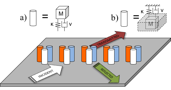
Figure 1: Schematic of the flexural wave grating problem: a line of clusters composed of multiple scatterers with possibly different mass, stiffness and damping properties within the cluster (but the same for each cluster). Each scatterer can be modeled as an attached mass-spring-dashpot system with properly tuned constants $M$, $\kappa$ and $\nu$. The schematic shows impedance models (a) and (b) of equation (3).

The paper is organised as follows; section II formulates the diffraction problem of a flexural plane wave by a periodic arrangement of clusters of $N$ scatterers. Section III defines the inverse grating problem and shows its solution and section IV applies the theory to the design of a negative refractor. Finally, section VI summarizes the work. Some mathematical results are derived in the Appendix.

II Diffraction by a periodic arrangement of point scatterers

II.1 Scattering by a single and a cluster of point impedances

The deflection $w({\bf r})$ on a two dimensional plate, ${\bf r}=x\hat{\bf x}+y\hat{\bf y}$, satisfies the Kirchhoff plate equation

$$D\big{(}\Delta^{2}w({\bf r})-k^{4}w({\bf r})\big{)}=0$$ (1)

where $k^{4}=\rho h\omega^{2}/D$, $D$ is the bending stiffness, $h$ is the plate thickness, and $\rho$ the density. Time harmonic dependence $e^{-\mathrm{i}\omega t}$ is assumed. Equation (1) holds everywhere on the infinite plate except where there are point impedances attached Evans and Porter (2007).

Consider first scattering from a single point attachment located at ${\bf r}={\bf R}$,

$$D\big{(}\Delta^{2}w({\bf r})-k^{4}w({\bf r})\big{)}=\mu w({\bf R})\delta({\bf r}-{\bf R}).$$ (2)

The attached oscillator impedance $\mu$ is modeled as single degree of freedom with mass $M$, spring stiffness $\kappa$ and damping coefficient $\nu$. Two possible models are

$$\mu=\begin{cases}\big{(}\frac{1}{M\omega^{2}}-\frac{1}{\kappa-\mathrm{i}\omega\nu}\big{)}^{-1},&(a),\\ M\omega^{2}-\kappa+\mathrm{i}\omega\nu,&(b).\end{cases}$$ (3)

In model (a) the mass is attached to the plate by a spring and damper acting in parallel Torrent et al. (2013). Model (b) assumes the mass is rigidly attached to the plate, and both are attached to a rigid foundation by the spring and damper in parallel Evans and Porter (2007). An important limit is a pointwise pinned plate, $w({\bf R})=0$, which corresponds to $\mu\to\infty$. The point attachments considered here are based on devices proposed for passive control of flexural waves using tuned vibration absorbers (TVA)s Brennan (1997, 1999); El-Khatib et al. (2005). A TVA, modeled as a point translational impedance, can be used to reduce vibration at a specific frequency or to control transmission and reflection of flexural waves in a beam Brennan (1999); El-Khatib et al. (2005). The alternative term vibration neutralizer Brennan (1997) is sometimes used. In the present context the point impedance, or TVA, is considered as a device for controlling the scattering of flexural waves in two-dimensional rather than in a 1D setting.

The total plate deflection is

$$w({\bf r})=w_{\text{in}}({\bf r})+BG({\bf r}-{\bf R})$$ (4)

where $w_{\text{in}}({\bf r})$ is the incident field and, by definition of the point impedance,

$$B=\mu w({\bf R}).$$ (5)

Also, $G$ is the Green’s function (see Appendix A)

$$G({\bf r})=C\big{(}H^{(1)}_{0}(kr)-H^{(1)}_{0}(\mathrm{i}kr)\big{)}$$ (6)

where $C=G({\bf 0})=\mathrm{i}/(8k^{2}D)$. Note that $H^{(1)}_{0}(\mathrm{i}kr)=-\frac{2\mathrm{i}}{\pi}K_{0}(kr)$. Setting ${\bf r}={\bf R}$ in (4) and using (5) yields

$$B=\frac{w_{\text{in}}({\bf R})}{\mu^{-1}-G({\bf 0})}.$$ (7)

If there are $N$ point scatterers located at ${\bf R}_{\alpha}=x_{\alpha}\hat{\bf x}+y_{\alpha}\hat{\bf y}$ with impedances $\mu_{\alpha}$, $\alpha=1,2,\ldots,N$, then the total field satisfies

$$D\big{(}\Delta^{2}w({\bf r})-k^{4}w({\bf r})\big{)}=\sum_{\alpha=1}^{N}\mu_{\alpha}w({\bf R}_{\alpha})\delta({\bf r}-{\bf R}_{\alpha}).$$ (8)

The solution is given by the incident field plus the field scattered by all the particles,

$$w({\bf r})=w_{\text{in}}({\bf r})+\sum_{\beta=1}^{N}B_{\beta}G({\bf r}-{\bf R}_{\beta}),\ \ B_{\beta}=\mu_{\beta}w({\bf R}_{\beta}).$$ (9)

Setting ${\bf r}={\bf R}_{\alpha}$ in (9) gives a linear system of $N$ equations for the amplitudes

$$\sum_{\beta=1}^{N}\big{(}\mu_{\alpha}^{-1}\delta_{\alpha\beta}-G({\bf R}_{\alpha}-{\bf R}_{\beta})\big{)}B_{\beta}=w_{\text{in}}({\bf R}_{\alpha}).$$ (10)

II.2 Scattering by an infinite set of impedances clusters

The above set of equations provides the solution for the multiple scattering problem of a given incident field on a cluster of small particles, once their position and their physical nature is properly described. We would like to know what happens now when this cluster is copied and distributed along a line and when the incident field is a plane wave of definite wavenumber ${\bf k}$:

$$w_{\text{in}}({\bf r})=e^{\mathrm{i}{\bf k}\cdot{\bf r}}.$$ (11)

This defines the grating scattering problem.

Specifically, the grating particle positions are

$${\bf R}_{\beta m}={\bf R}_{\beta}+{\bf R}_{m}$$ (12)

where $\beta=1,2,...,N$ defines the cluster element while ${\bf R}_{m}=m{\bf a}$, $m\in\mathbb{Z}$, covers the infinite periodic grating. The total field is then

$$w({\bf r})=w_{\text{in}}({\bf r})+\sum_{\beta=1}^{N}\sum_{{\bf R}_{m}}\mu_{\beta}w({\bf R}_{\beta m})G({\bf r}-{\bf R}_{\beta m}).$$ (13)

It is assumed that the cluster-to-cluster relation for the total field satisfies the same phase relation as the incident field,

$$w({\bf R}_{\beta m})=w({\bf R}_{\beta})e^{\mathrm{i}{\bf k}\cdot{\bf R}_{m}}.$$ (14)

This crucial identity implies that the total field can be represented in terms of $N$ amplitudes, $\{B_{\beta},\,\beta=1,2,\ldots,N\}$,

$$w({\bf r})=e^{\mathrm{i}{\bf k}\cdot{\bf r}}+\sum_{\beta=1}^{N}B_{\beta}\sum_{{\bf R}_{m}}e^{\mathrm{i}{\bf k}\cdot{\bf R}_{m}}G({\bf r}-{\bf R}_{\beta}-{\bf R}_{m}).$$ (15)

The amplitudes can be found by the same method as for the single cluster. Thus, setting ${\bf r}={\bf R}_{\alpha}$ in (15) gives a linear system of $N$ equations

$$\sum_{\beta=1}^{N}\big{(}\mu_{\alpha}^{-1}\delta_{\alpha\beta}-\chi_{\alpha\beta}\big{)}B_{\beta}=e^{\mathrm{i}{\bf k}\cdot{\bf R}_{\alpha}}$$ (16)

with

$$\chi_{\alpha\beta}=\sum_{{\bf R}_{m}}e^{\mathrm{i}{\bf k}\cdot{\bf R}_{m}}G({\bf R}_{\alpha}-{\bf R}_{\beta}-{\bf R}_{m}).$$ (17)

II.3 Solution of the forward scattering grating problem

The $N$-cluster repeats along a line,

$${\bf R}_{m}=ma\hat{\bf x},\ m\in\mathbb{Z},$$ (18)

and therefore we can use the lattice sum identity (see Appendix)

$$\sum_{{\bf R}_{m}}e^{\mathrm{i}{\bf k}\cdot{\bf R}_{m}}G({\bf r}-{\bf R}_{m}) =G_{0}\sum_{n\in\mathbb{Z}}e^{\mathrm{i}(k_{x}+g_{n})x}\Big{(}\frac{e^{-\zeta_{-}|y|}}{\zeta_{-}}-\frac{e^{-\zeta_{+}|y|}}{\zeta_{+}}\Big{)},$$ (19a)

$$G_{0}=\frac{1}{4Dk^{2}a},\ \ g_{n} =\frac{2\pi}{a}n,\ \ \zeta_{\pm}=((k_{x}+g_{n})^{2}\pm k^{2})^{1/2},$$ (19b)

where $\operatorname{Im}\zeta_{-}\leq 0$. Specifically, (19) implies that the total field (15) is

$$w({\bf r})=e^{\mathrm{i}{\bf k}\cdot{\bf r}}+G_{0}\sum_{\beta=1}^{N}B_{\beta}\sum_{n\in\mathbb{Z}}e^{\mathrm{i}(k_{x}+g_{n})(x-x_{\beta})}\Big{(}\frac{e^{-\zeta_{-}|y-y_{\beta}|}}{\zeta_{-}}-\frac{e^{-\zeta_{+}|y-y_{\beta}|}}{\zeta_{+}}\Big{)}$$ (20)

where the $N$ coefficients $B_{\beta}$ follow from eq. (16) and (17) with (instead of the general form (10))

$$\chi_{\alpha\beta}=G_{0}\sum_{n\in\mathbb{Z}}e^{\mathrm{i}(k_{x}+g_{n})(x_{\alpha}-x_{\beta})}\Big{(}\frac{e^{-\zeta_{-}|y_{\alpha}-y_{\beta}|}}{\zeta_{-}}-\frac{e^{-\zeta_{+}|y_{\alpha}-y_{\beta}|}}{\zeta_{+}}\Big{)}.$$ (21)

This provides a much more computationally efficient expression than the slowly convergent (17). Note that the semi-analytical form for $\chi_{\alpha\beta}$ is a consequence of the fact that the Green’s function can be expressed as a Fourier integral. This indicates that the same procedure used in the Appendix would apply to other wave systems for which the Green’s function does not have a closed form solution.

The $\zeta_{+}$ terms in the total field (20) all decay exponentially away from the line, while the $\zeta_{-}$ terms also decay except for those for which $\zeta_{-}$ is imaginary. The latter define the finite set of propagating modes, ${\mathbb{P}}$ with $N_{\text{P}}$ elements, defined as

$${{\mathbb{P}}}=\{n\in{\mathbb{Z}}:\,|k_{x}+g_{n}|<k\}.$$ (22)

These are the values for which $\zeta_{-}$ is purely (negative) imaginary and they correspond to the far-field diffraction orders of the grating, all others are strictly near-field. Note that ${{\mathbb{P}}}$ always includes the value $n=0$, so that $N_{\text{P}}\geq 1$.

Let $\theta_{0}\in[0,\frac{\pi}{2}]$ be the angle of incidence relative to the grating direction, so that

$${\bf k}=k_{x}\hat{\bf x}+k_{y}\hat{\bf y}=k\cos\theta_{0}\hat{\bf x}+k\sin\theta_{0}\hat{\bf y}.$$ (23)

In particular, $k_{x}=k\cos\theta_{0}$ implies that the direction of the propagating mode $n$ is defined by the angle

$$\theta_{n}=\cos^{-1}\big{(}\cos\theta_{0}+\frac{2\pi}{ka}n\big{)},\ \ \theta_{n}\in(0,\pi),\ \ n\in{\mathbb{P}}.$$ (24)

Hence, ${\mathbb{P}}$ can be considered as the set of $n$ for which $\theta_{n}$ is real valued. The far-field diffracted displacement is

$$w({\bf r})=e^{\mathrm{i}{\bf k}\cdot{\bf r}}+\frac{\mathrm{i}G_{0}}{k}\sum_{\beta=1}^{N}B_{\beta}\sum_{n\in{\mathbb{P}}}\frac{1}{\sin\theta_{n}}e^{\mathrm{i}k[(x-x_{\beta})\cos\theta_{n}+|y-y_{\beta}|\sin\theta_{n}]},\ \ |y|\to\infty.$$ (25)

The individual diffracted modes are therefore

$$w({\bf r})=\begin{cases}\sum_{n\in{\mathbb{P}}}t_{n}e^{\mathrm{i}{\bf k}_{n}^{+}\cdot{\bf x}},&y\to\infty,\\ \sum_{n\in{\mathbb{P}}}r_{n}e^{\mathrm{i}{\bf k}_{n}^{-}\cdot{\bf x}},&y\to-\infty,\end{cases}$$ (26)

where ${\bf k}_{n}^{+}$, ${\bf k}_{n}^{-}$, are the wavenumbers of the transmitted and reflected waves, respectively,

$${\bf k}_{n}^{\pm}=k\cos\theta_{n}\hat{\bf x}\pm k\sin\theta_{n}\hat{\bf y},\ \ n\in\mathbb{P}$$ (27)

and the $2N_{\text{P}}$ transmission and reflection coefficients follow from (25) and (26) as

$$\left.\begin{matrix}t_{n}-\delta_{n0}\\ r_{n}\end{matrix}\right\}=\frac{\mathrm{i}G_{0}}{k\sin\theta_{n}}\sum_{\beta=1}^{N}B_{\beta}\times\begin{cases}e^{-\mathrm{i}{\bf k}_{n}^{+}\cdot{\bf R}_{\beta}},\\ e^{-\mathrm{i}{\bf k}_{n}^{-}\cdot{\bf R}_{\beta}},\end{cases}\ \ n\in{\mathbb{P}}.$$ (28)

Note that ${\bf k}_{0}^{+}={\bf k}$, the incident wavevector, and that conservation of energy requires

$$\sum_{n\in{\mathbb{P}}}\big{(}|r_{n}|^{2}+|t_{n}|^{2}\big{)}\sin\theta_{n}\leq\sin\theta_{0}$$ (29)

with equality if the impedances $\mu_{\alpha}$ are all real valued (no damping).

Finally, we note that if all the scatterers lie along a line parallel to the $x-$axis, i.e. $y_{\beta}=b$ $\forall\beta$ for some $b$, then

$$t_{n}-\delta_{n0}=r_{n}e^{-\mathrm{i}2kb\sin\theta_{n}},\ \ n\in{\mathbb{P}}.$$ (30)

The number of independent scattering coefficients is therefore greatly reduced. This redundancy has implications in the selection of scatterer positions for the inverse grating problem, considered next.

III The inverse grating problem

We are interested in controlling the reflection and transmission coefficients through (inverse) design of the grating. For instance, Figure 2 shows a grating that makes all but one of the scattered modes vanish, in this case all except the $n=-1$ mode. Specific designs for this type of grating are given below. The design and control is achieved using the combined degrees of freedom of the cluster spatial distribution, ${\bf R}_{m}$, the scatterers’ positions, ${\bf R}_{\alpha}$, and their impedances, $\mu_{\alpha}$. We consider the incidence direction $\theta_{0}$ and the nondimensional frequency $ka$ as given quantities. The inverse problem as posed is still highly non-unique, since there could be multiple configurations that achieve the same objective. We therefore concentrate on specific geometrical configurations for the cluster distributions, such as a cluster of $N=3$ scatterers positioned at the vertices of a triangle or along a line. This allows us to focus on the inverse problem of finding the impedances, and specifically on making them passive but with as little damping as possible so that all of the incident energy is channeled into the selected mode diffraction.

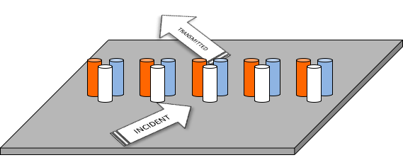
Figure 2: A grating which channels all of the wave energy into the $n=-1$ diffracted mode.

III.1 Inverting for impedances

Equation (16), written in matrix form is

$${{\bf E}}={\bf M}{\bf B}$$ (31)

where the $N\times N$ matrix $\bf M$ follows from (16) and the $N-$vector $\bf E$ contains the incident wave amplitudes at the $N$ scatterer positions,

$${\bf M}={\boldsymbol{\mu}}^{-1}-{\boldsymbol{\chi}},\ \ \ {\bm{\mu}}=\begin{pmatrix}\mu_{1}&&&0\\ &\mu_{2}&&\\ &&\ddots&\\ 0&&&\mu_{N}\end{pmatrix},\ \ \ {\bf E}=\begin{pmatrix}e^{\mathrm{i}{\bf k}\cdot{\bf R}_{1}}\\ e^{\mathrm{i}{\bf k}\cdot{\bf R}_{2}}\\ \vdots\\ e^{\mathrm{i}{\bf k}\cdot{\bf R}_{N}}\end{pmatrix}.$$ (32)

The elements of the $N\times N$ matrix $\boldsymbol{\chi}$ are defined by the infinite sums (20). Using the fact that $\boldsymbol{\mu}$ is diagonal we can reconsider (31) as an equation for $\boldsymbol{\mu}$ in terms of the amplitudes $B_{\alpha}$,

$$\mu^{-1}_{\alpha}=\big{(}e^{\mathrm{i}{\bf k}\cdot{\bf R}_{\alpha}}+{\bf e}_{\alpha}^{T}{\boldsymbol{\chi}}{\bf B}\big{)}/B_{\alpha}$$ (33)

where the elements of the $N-$vector ${\bf e}_{\alpha}$ are zero except for the $\alpha^{\text{th}}$, which is unity. In order to proceed we need to obtain the amplitudes ${\bf B}$.

The goal is to control transmission coefficients, so we therefore collect the transmission and reflection coefficients into a $2N_{\text{P}}-$vector denoted by ${\bf T}=[(t_{n}-\delta_{n0})\frac{\sin\theta_{n}}{\sin\theta_{0}},r_{n}\frac{\sin\theta_{n}}{\sin\theta_{0}}]^{T}$ with $n\in\mathbb{P}$. The vector length, $2N_{\text{P}}$, depends on the number of diffraction orders. Then, we may rewrite the equations for the transmission and reflection coefficients, (28), as

$${\bf T}={\bf S}{\bf B}$$ (34)

with ${\bf S}$, a $2N_{\text{P}}\times N$ matrix, collecting the exponential terms related to scatterer positions

$${\bf S}=\frac{\mathrm{i}G_{0}}{k\sin\theta_{0}}\begin{pmatrix}e^{-\mathrm{i}{\bf k}_{0}^{+}\cdot{\bf R}_{1}}&e^{-\mathrm{i}{\bf k}_{0}^{+}\cdot{\bf R}_{2}}&\cdots&e^{-\mathrm{i}{\bf k}_{0}^{+}\cdot{\bf R}_{N}}\\ e^{-\mathrm{i}{\bf k}_{0}^{-}\cdot{\bf R}_{1}}&e^{-\mathrm{i}{\bf k}_{0}^{-}\cdot{\bf R}_{2}}&\cdots&e^{-\mathrm{i}{\bf k}_{0}^{-}\cdot{\bf R}_{N}}\\ e^{-\mathrm{i}{\bf k}_{-1}^{+}\cdot{\bf R}_{1}}&e^{-\mathrm{i}{\bf k}_{-1}^{+}\cdot{\bf R}_{2}}&\cdots&e^{-\mathrm{i}{\bf k}_{-1}^{+}\cdot{\bf R}_{N}}\\ e^{-\mathrm{i}{\bf k}_{-1}^{-}\cdot{\bf R}_{1}}&e^{-\mathrm{i}{\bf k}_{-1}^{-}\cdot{\bf R}_{2}}&\cdots&e^{-\mathrm{i}{\bf k}_{-1}^{-}\cdot{\bf R}_{N}}\\ \vdots&\vdots&\vdots&\vdots\\ e^{-\mathrm{i}{\bf k}_{n_{P}}^{+}\cdot{\bf R}_{1}}&e^{-\mathrm{i}{\bf k}_{n_{P}}^{+}\cdot{\bf R}_{2}}&\cdots&e^{-\mathrm{i}{\bf k}_{n_{P}}^{+}\cdot{\bf R}_{N}}\\ e^{-\mathrm{i}{\bf k}_{n_{P}}^{-}\cdot{\bf R}_{1}}&e^{-\mathrm{i}{\bf k}_{n_{P}}^{-}\cdot{\bf R}_{2}}&\cdots&e^{-\mathrm{i}{\bf k}_{n_{P}}^{-}\cdot{\bf R}_{N}}\end{pmatrix},$$ (35)

where $n_{P}$ indicates the $N_{\text{P}}^{\text{th}}$ diffracted mode.

We focus on the inverse grating problem of eliminating all but one of the $2N_{\text{P}}$ transmission and reflection coefficients. Suppose we want all coefficients to vanish except, for instance, $t_{m}$ or $r_{m}$, then (34) provides $2N_{\text{P}}-1$ identities. In order to have a solvable linear but not overdetermined system we require that the number of unknowns equals the number of knowns, implying a relation between the number of scatterers and the number of diffracted modes:

$$N=2N_{\text{P}}-1.$$ (36)

The magnitude of the remaining coefficient must satisfy (29), implying

$$\hat{\bf T}=\hat{\bf S}{\bf B}$$ (37)

where the $N-$vector $\hat{\bf T}$ ($N=2N_{\text{P}}-1$ vector) follows from ${\bf T}$ by removing the row for $t_{m}$ or $r_{m}$, and the square $N\times N$ matrix $\hat{\bf S}$ is obtained from the $2N_{\text{P}}\times 2N_{\text{P}}-1$ matrix ${\bf S}$ by removing the row corresponding to the unconstrained coefficient ($t_{m}$ or $r_{m}$). The $N$ scatterer amplitudes are therefore

$${\bf B}={\hat{\bf S}}^{-1}\hat{\bf T}.$$ (38)

It is important to note that we are assuming a non-singular ${\hat{\bf S}}$; the possibility and implications of ${\hat{\bf S}}$ being singular are discussed later. Substituting $\bf B$ into (33) yields the impedances in terms of the transmission/reflection vector $\hat{\bf T}$ as

$$\mu^{-1}_{\alpha}=\frac{e^{\mathrm{i}{\bf k}\cdot{\bf R}_{\alpha}}+{\bf e}_{\alpha}^{T}{\boldsymbol{\chi}}\hat{\bf S}^{-1}\hat{\bf T}}{{\bf e}_{\alpha}^{T}\hat{\bf S}^{-1}\hat{\bf T}},\ \ \alpha=1,2,\ldots,N.$$ (39)

Equation (39) provides a simple inversion procedure at a given frequency for a given arrangement of scatterers the number of which, $N$, is related to the number of diffraction orders, $N_{\text{P}}$, by equation (36). The latter implies that the number of scatterers is odd. The solution (39) yields complex values for the impedances. A realistic solution requires the further conditions that the impedances are passive, which is the case only if $\operatorname{Im}\mu_{\alpha}\geq 0$ $(\operatorname{Im}\mu_{\alpha}^{-1}\leq 0)$ for all $\alpha=1,2\ldots,N$.

An explicit solution follows for the case in which all coefficients vanish except for the fundamental transmission $t_{0}$. Then $\hat{\bf T}={\bf 0}$ implying, from (39), that $\mu_{\alpha}=0$. The solution is trivial: there is no grating. For every other case, no matter which of the remaining $N=2N_{\text{P}}-1$ coefficients is chosen as the one that is non-zero, the $N-$vector $\hat{\bf T}$ has the same form, viz.

$$\hat{\bf T}=(-1,\,0,\,0,\ldots,0)=-{\bf e}_{1}.$$ (40)

Equation (39) therefore simplifies to

$$\mu^{-1}_{\alpha}=\frac{{\bf e}_{\alpha}^{T}{\boldsymbol{\chi}}\hat{\bf S}^{-1}{\bf e}_{1}-e^{\mathrm{i}{\bf k}\cdot{\bf R}_{\alpha}}}{{\bf e}_{\alpha}^{T}\hat{\bf S}^{-1}{\bf e}_{1}},\ \ \alpha=1,2,\ldots,N.$$ (41)

In summary, if the impedances satisfy (41) then all but one of the transmission and reflection coefficients vanish.

The matrix $\hat{\bf S}$ is invertible if and only if it is full rank, i.e. with $N$ linearly independent rows. If the scatterers are positioned along a line parallel to the $x-$axis, at the common coordinate $y_{\beta}=b$, then referring to (35), $e^{-\mathrm{i}{\bf k}_{n}^{+}\cdot{\bf R}_{\alpha}}=e^{-\mathrm{i}{\bf k}_{n}^{-}\cdot{\bf R}_{\alpha}}e^{-\mathrm{i}2kb\sin\theta_{n}}$. This implies that $\hat{\bf S}$ has at most $(N-1)/2$ linearly dependent rows, and therefore the rank of the matrix falls precipitously from $N$ to $\frac{1}{2}(N+1)=N_{\text{P}}$, see eq. (36). Despite this singularity, it may happen that the expression (41) has a finite value by virtue of the fact this it contains $\hat{\bf S}^{-1}{\bf e}_{1}$ in the numerator and in the denominator. Also, $\hat{\bf S}^{-1}{\bf e}_{1}$ itself can be finite even though $\hat{\bf S}$ is singular, as is the case in the example in Appendix B. Finally, the obvious exception to this discussion is the simplest, $N=1$, considered next.

IV Examples and applications

Following the theoretical developments for the inverse design of gratings, outlined in section III, we now present and discuss examples and applications. We first focus on the simple case of $N=1$, when only one diffracted mode exists, i.e. $n\in\mathbb{P}=\{0\}$. Next, a more complex design for $N=3$ (with $\mathbb{P}=\{-1;0\}$) will be developed with particular focus on the inverse design of the cluster. This configuration will be used to find scatterer configurations resulting in the negative refraction of waves at the grating.

The negative refractor consists in a grating that diverts an incoming wave in such a way that if the angle the wave makes with the $x-$axis is $\theta_{0}$ that of the transmitted wave is $\pi-\theta_{0}$. This is indeed the “refraction” version of the retroreflector, in which the incident wave is retroreflected. From the diffraction point of view we assume that the selected incident angle $\theta_{0}$ allows for two diffracted modes $\mathbb{P}=\{-1;0\}$. We also want the angle of the $n=-1$ mode to be $\theta_{n}=\pi-\theta_{0}$, therefore, using $k=\frac{2\pi}{\lambda}$ equation (24) gives

$$-\cos\theta_{0}=\cos\theta_{0}-\frac{\lambda}{a}$$ (42)

which sets up the ratio $\lambda/a=2\cos\theta_{0}$ (or $ka=\pi\sec\theta_{0}$). A configuration of $N=3$ scatterers will be used to demonstrate the negative refractor.

IV.1 The simple grating: $N=1$

By assumption, the fundamental is the only diffracted order and the only transmission/reflection coefficients are related by $t_{0}=r_{0}+1$, assuming with no loss in generality that it is positioned at ${\bf R}_{1}={\bf 0}$. Equation (41), the condition for total reflection $(t_{0}=0\,\Rightarrow\,r_{0}=-1)$, reduces to a scalar relation

$$\mu^{-1}=\chi-\frac{\mathrm{i}G_{0}}{k\sin\theta_{0}}$$ (43)

where $\chi=\chi_{\alpha\alpha}$ follows from (21). In particular Evans and Porter (2007) since ${\mathbb{P}}=\{0\}$,

$$\chi-\frac{\mathrm{i}G_{0}}{k\sin\theta_{0}}\equiv\chi_{1}=\frac{-G_{0}}{k\sqrt{1+\cos^{2}\theta_{0}}}+G_{0}\sum_{n\in\mathbb{Z}\backslash 0}\Big{(}\frac{1}{\sqrt{(k_{x}+g_{n})^{2}-k^{2}}}-\frac{1}{\sqrt{(k_{x}+g_{n})^{2}+k^{2}}}\Big{)}$$ (44)

where $\chi_{1}$ is real. Total reflection can therefore be achieved with real impedance $\mu=\chi_{1}^{-1}$, a result previously obtained in Evans and Porter (2007).

Since there is only one scattering coefficient in this case (because $t_{0}=r_{0}+1$), it is of interest to see what other values of $t_{0}$ can be achieved. Instead of using (40) we retain $t_{0}\neq 0$ and set $\hat{T}=t_{0}-1$. Equation (39) then simplifies to

$$\mu^{-1}=\frac{\mathrm{i}G_{0}t_{0}}{k\sin\theta_{0}(t_{0}-1)}+\chi_{1}.$$ (45)

Equation (45) provides an explicit expression for the impedance for a given incidence direction $\theta_{0}$, lattice spacing $a$, wavenumber $k$ and transmission $t_{0}$. The impedance is complex valued, indicating damping is necessary, except for the two limiting values $t_{0}=0$, discussed above, and $t_{0}=1$ which is the trivial limit of $\mu=0$, i.e.  no grating.

What other values of $t_{0}$ can be achieved with a passive impedance? Recall that a passive impedance maintains or dissipates energy, as opposed to an active impedance which requires an external energy source. The impedance is passive iff $\operatorname{Im}\mu^{-1}\leq 0$, e.g. see (3). Equation (45) gives a passive $\mu$ iff $\operatorname{Re}\frac{t_{0}}{t_{0}-1}\leq 0$. Hence,

$$t_{0}=|t_{0}|e^{\mathrm{i}\phi},\ \ |t_{0}|\leq\cos\phi\ \Leftrightarrow\ \text{passive }\ \mu.$$ (46)

In addition to the limits $t_{0}=1$ and $t_{0}=0$ discussed above, this provides the entire range of transmission coefficients achievable with $N=1$.

IV.2 The next simplest grating: $N=3$

There are two diffracted modes, $\mathbb{P}=\{-1;0\}$, if the incidence angle $\theta_{0}$ is large enough, which is now assumed. Following the discussion in section III we will need three scatterers, $N=3$, in order to control three out of four reflection and transmission coefficients. With the goal of designing a negative refractor we want the only propagating mode, among all transmitted through or reflected from the grating, be the transmitted $n=-1$ order. A grating that sends all of the incident energy into the transmitted $n=-1$ mode has matrix $\hat{\bf S}$,

$$\hat{\bf S}=\frac{\mathrm{i}G_{0}}{k\sin\theta_{0}}\begin{pmatrix}e^{-\mathrm{i}{\bf k}_{0}^{+}\cdot{\bf R}_{1}}&e^{-\mathrm{i}{\bf k}_{0}^{+}\cdot{\bf R}_{2}}&e^{-\mathrm{i}{\bf k}_{0}^{+}\cdot{\bf R}_{3}}\\ e^{-\mathrm{i}{\bf k}_{0}^{-}\cdot{\bf R}_{1}}&e^{-\mathrm{i}{\bf k}_{0}^{-}\cdot{\bf R}_{2}}&e^{-\mathrm{i}{\bf k}_{0}^{-}\cdot{\bf R}_{3}}\\ e^{-\mathrm{i}{\bf k}_{-1}^{-}\cdot{\bf R}_{1}}&e^{-\mathrm{i}{\bf k}_{-1}^{-}\cdot{\bf R}_{2}}&e^{-\mathrm{i}{\bf k}_{-1}^{-}\cdot{\bf R}_{3}}\end{pmatrix}.$$ (47)

We consider two particular geometrical setups for $N=3$ clusters, namely a linear and triangular cluster, as shown in Figure 3. In each case we parametrize the cluster by the spacing between the scatterers and the rotation angle of the cluster, $d$ and $\theta_{d}$, respectively.

Figure 3: Two investigated cluster configurations: (a) linear and (b) triangular.

The positions of the scatterers in the cluster are then: ${\bf R}_{1}=(0,0)$ and $\bm{R}_{2\atop 3}=\pm d(\cos\theta_{d},\sin\theta_{d})$, $d>0$ for the linear cluster; and ${\bf R}_{1}=\frac{d}{\sqrt{3}}\ \big{(}-\sin\theta_{d},\cos\theta_{d}\big{)}$ and ${\bf R}_{2\atop 3}=\frac{d}{\sqrt{3}}\ \big{(}\sin(\theta_{d}\mp\frac{\pi}{6}),-\cos(\theta_{d}\mp\frac{\pi}{6})\big{)}$ for the triangular cluster.

The design process for a grating consists of finding scatterers’ impedances and positions $(d,\theta_{d})$. Among all possible solutions we are interested in passive cluster configurations, i.e. $\operatorname{Im}\mu_{\alpha}>0$ for all $\alpha$, that correspond to the largest possible transmission coefficient $|t_{-1}|$. The latter would imply that possibly large portion of energy of the incident wave is sent into the transmitted $n=-1$ mode, resulting in the negative refractor. From a practical perspective, a particularly interesting cluster setup would satisfy $\operatorname{Im}\mu_{\alpha}=0$, resulting in spring-mass configurations of the scatterers only (no damping).

In the following examples we assume the incident wavevector $k=\pi/(a\ \cos\theta_{0})$ at angle $\theta_{0}=\pi/4$. In each case all but $t_{-1}$ reflection and transmission coefficients in $\hat{{\bf T}}$ are set to zero. We also assume, for simplicity, $D=1$ and $a=1$.

IV.3 Numerical examples

IV.3.1 Results for the linear cluster

We begin by inverting $\hat{{\bf S}}$ from (47) and using (39) to solve for impedances. Figures 4 and 5 show, respectively, the imaginary and real parts of the complex-valued impedance $\mu_{1}$ and $\mu_{2}$ ($\mu_{3}$ is similar to $\mu_{2}$ due to the symmetry of the cluster) for $\theta_{d}\in(0,2\pi)$ and $d\in(0,a)$. As we are interested in passive solutions only, the plots in Figures 4 and 5 are limited to $(d,\theta_{d})$ combinations resulting in $\operatorname{Im}\mu_{\alpha}>0$ for respective scatterers independently. A cluster with passive damping properties can only be constructed by selecting scatterers positions corresponding to impedances satisfying $\operatorname{Im}\mu_{\alpha}>0$ for all $\alpha$. Those combinations of $(d,\theta_{d})$, with the values of $|t_{-1}|$ are shown in Figure 6.

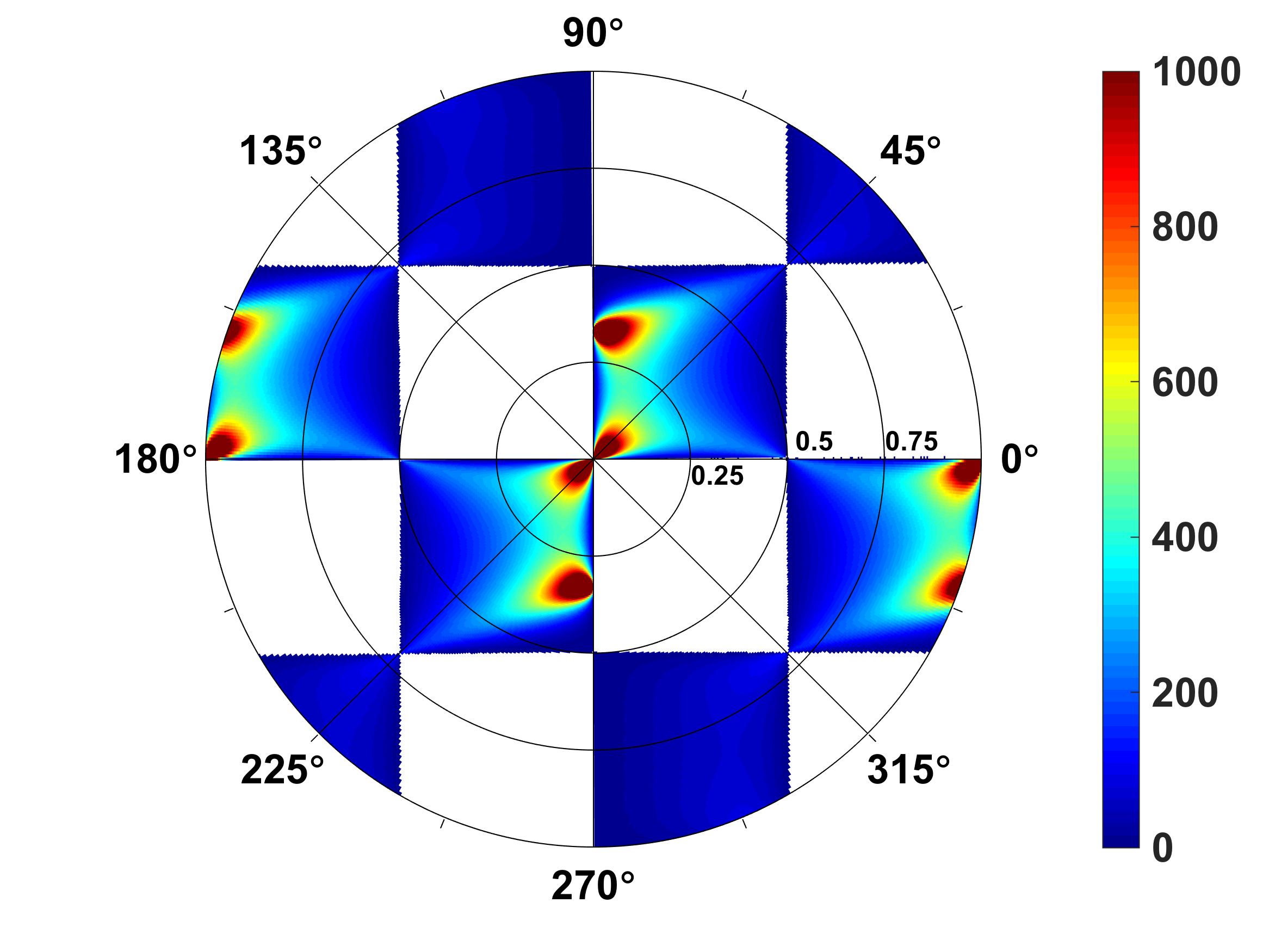
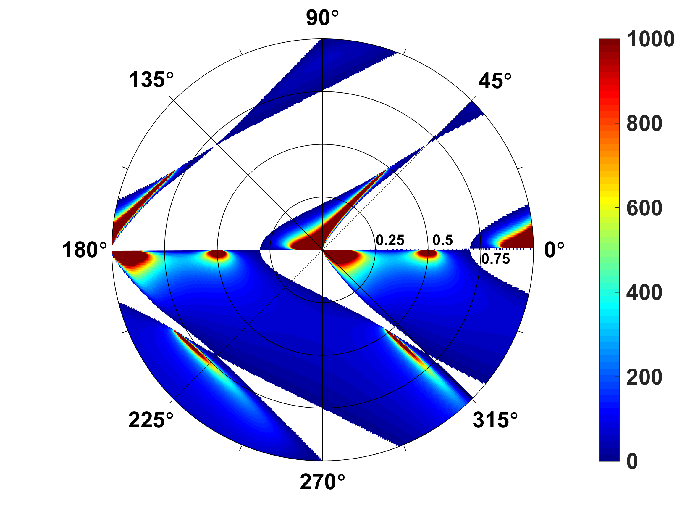
Figure 4: Imaginary parts of the complex-valued impedance $\mu_{1}$ (left) and $\mu_{2}$ (right), in units of $a^{2}/D$, as functions of $d$ and $\theta_{d}$ for a fixed incident wavevector angle $\theta_{0}=\pi/4$ and $k=\pi/(a\ \cos\theta_{0})$ (for $a=1$), for the $N=3$ linear cluster negative refractor. The plot only shows regions for which the impedances are passive: $\operatorname{Im}\mu_{1},\mu_{2}\geq 0$.

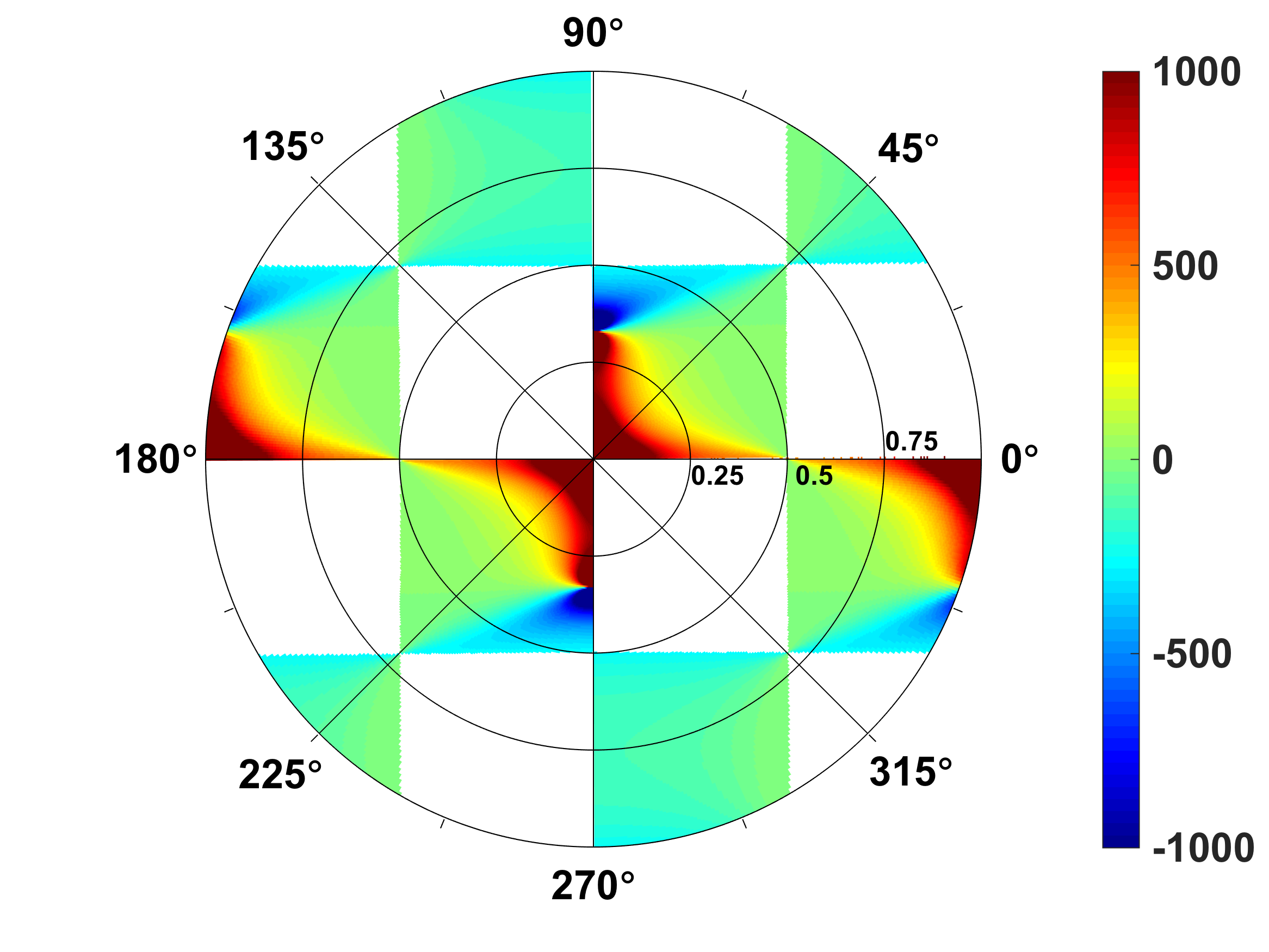
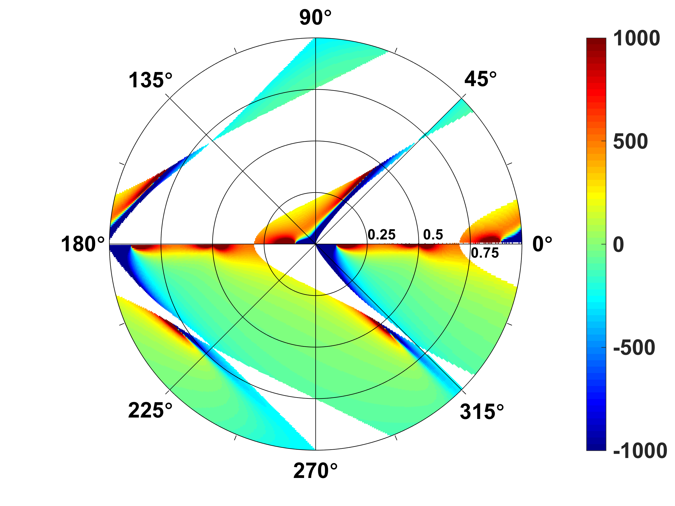
Figure 5: Real parts of the impedances $\mu_{1}$ (left) and $\mu_{2}$ (right), in units of $a^{2}/D$, as functions of $d$ and $\theta_{d}$ for incident wavevector angle $\theta_{0}=\pi/4$ and $k=\pi/(a\ \cos\theta_{0})$ (for $a=1$), for the $N=3$ linear cluster negative refractor. The plot is restricted to passive impedances, see Fig. 4.

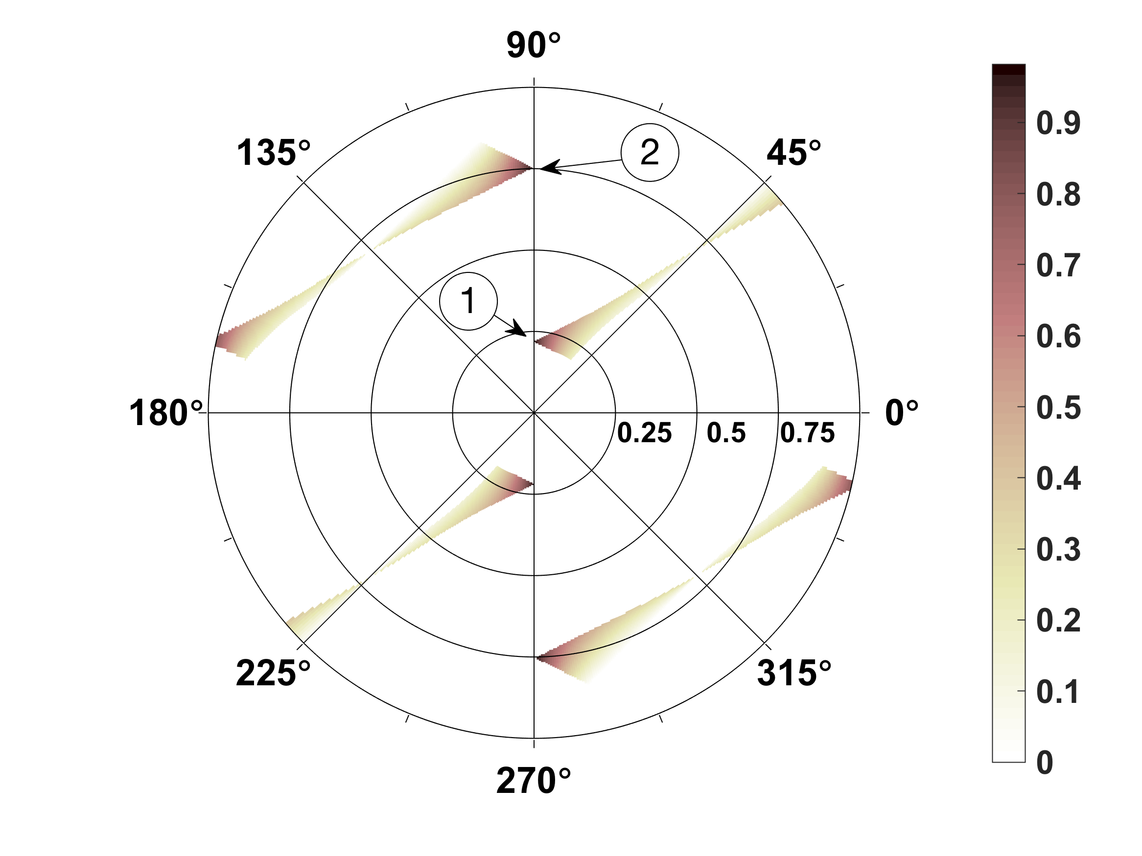
Figure 6: Magnitude of the transmission coefficient $t_{-1}$ for the designed linear $3-$cluster negative refractor as a function of $(d,\theta_{d})$ plotted in polar coordinates. The regions shown corresponding to passive $\mu_{\alpha}$ for all $\alpha$, and labels on the selected points are consistent with table 1.

Cluster configurations corresponding to the highest values of $|t_{-1}|$ are preferred. The largest values of $|t_{-1}|$ in Figure 6 are obtained for clusters oriented vertically. Interestingly, the same figure indicates that zero transmission points occur at cluster angles perpendicular or parallel to the incident wavefront. For detailed investigation we select $(d,\theta_{d})$ pairs with large values of $|t_{-1}|$, namely $(0.225,\pi/2)$ and $(0.751,\pi/2)$. The corresponding impedances of the scatterers are listed in table 1. Note that the the two selected clusters differ only in the (vertical) spacing $d$, and that the difference between the two values, $d_{2}-d_{1}\approx 0.5$ corresponds to a phase change of $k_{y}(d_{2}-d_{1})\approx\pi/2$. Other points with the same high transmission correspond to $2\pi$ phase change in the $y$ direction, and are situated outside the region shown above (and below) clusters \raisebox{-.9pt} {1}⃝ and \raisebox{-.9pt} {2}⃝.

It might seem surprising that the optimal orientation of the linear cluster is vertical, since it is clear from (47) and the identities ${\bf k}_{-1}^{\pm}=-{\bf k}_{0}^{\mp}$ for the negative refractor, that if the three scatterers are on a line parallel to the $y-$axis then the second and third rows of $\hat{\bf S}$ are identical, making the matrix singular. However, it is shown in Appendix B that even though the matrix $\hat{\bf S}$ is indeed singular for $\theta_{d}=\pi/2$, the vector $\hat{\bf S}^{-1}{\bf e}_{1}$ which appears in (41) remains finite. The symmetry of the $3-$cluster for $\theta_{d}=\pi/2$ also implies that the matrix $\boldsymbol{\chi}$ of (17) is symmetric with only three independent elements, since $\chi_{11}=\chi_{22}=\chi_{33}$ and $\chi_{12}=\chi_{13}$.

Using impedances and cluster configurations from table 1, reflection and transmission coefficients, and plate displacements at the scatterers were computed for a wide range of $k\times a$. Results for the linear clusters \raisebox{-.9pt} {1}⃝ and \raisebox{-.9pt} {2}⃝ are shown in Figures 7 and 8, respectively.

Brown solid horizontal lines in Figures 7 and 8 (and later) define the energy conservation threshold $\sin\theta_{0}$ of eq. (29), while the brown dotted lines depict the energy associated with all propagation modes, i.e. the left hand side (LHS) of eq. (29). Conservation of energy requires that the continuous line is above the dotted one, which is always the case in the examples considered.

Figures 7 and 8 illustrate relatively high transmission coefficients (approximately $0.97$) for the $n=-1$ diffracted mode for the linear clusters, meaning that almost all energy incident on the grating is converted to this mode. Of the two configurations, \raisebox{-.9pt} {1}⃝ is more broadband, i.e. it achieves similar transmission properties for a wider range of $k\times a$.

Table 1: Selected cluster configurations for $N=3$, see Figure 3.

Cluster:	linear \raisebox{-.9pt} {1}⃝	linear \raisebox{-.9pt} {2}⃝	triangular \raisebox{-.9pt} {1}⃝	triangular \raisebox{-.9pt} {2}⃝
$(d,\theta_{d})$	$(0.225,\pi/2)$	$(0.751,\pi/2)$	$(0.7484,0.9237)$	$(1.438,1.281)$
$\mu_{1}a^{2}/D$	$9.7253+0.2878\mathrm{i}$	$-1.2684+0.0095\mathrm{i}$	$-1.8861+0.0141\mathrm{i}$	$-3.4707+0.1240\mathrm{i}$
$\mu_{2}a^{2}/D$	$2.2272+0.0022\mathrm{i}$	$-0.8477+0.0043\mathrm{i}$	$-0.6507+0.5238\mathrm{i}$	$-4.0771+0.0308\mathrm{i}$
$\mu_{3}a^{2}/D$	$2.1609+0.0370\mathrm{i}$	$-0.8308+0.0120\mathrm{i}$	$1.5165+0.0588\mathrm{i}$	$-0.4929+0.3752\mathrm{i}$
	$\times 10^{2}$	$\times 10^{2}$	$\times 10^{2}$	$\times 10^{2}$

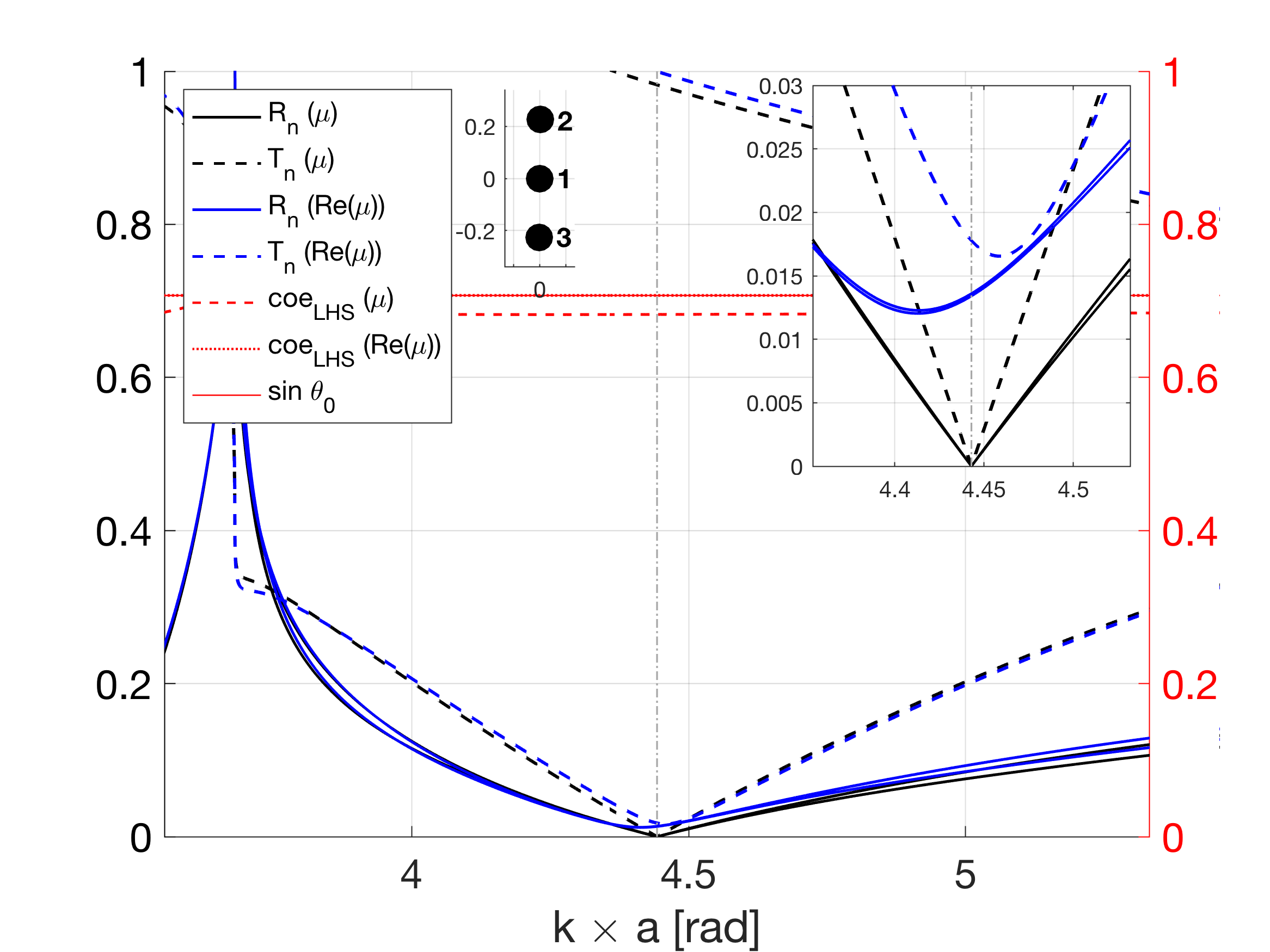
Figure 7: Reflection and transmission coefficients for the linear cluster ① computed for impedances given in table 1 for complex values of $\mu_{\alpha}$ and for $\operatorname{Im}\mu_{\alpha}=0$. The vertical dash-dot line at $k\times a=\pi/\cos\pi/4$ indicates the operating point of the grating.

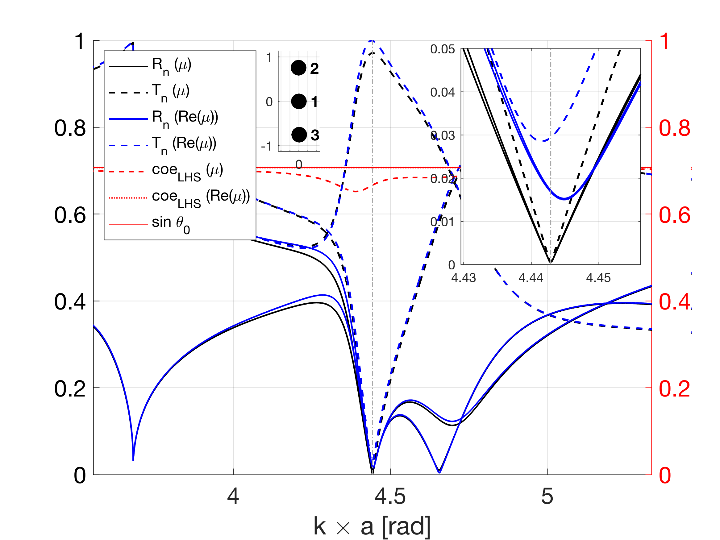
Figure 8: Reflection and transmission coefficients for the linear cluster ② using impedances from table 1 for complex values of $\mu_{\alpha}$ and for $\operatorname{Im}\mu_{\alpha}=0$. The vertical dash-dot line at $k\times a=\pi/\cos\pi/4$ indicates the operating frequency of the grating.

We next relax the restrictions on the impedances given in table 1 by using only their real parts, with the results shown in Figures 7 and 8 for linear clusters \raisebox{-.9pt} {1}⃝ and \raisebox{-.9pt} {2}⃝, respectively. It can be seen that for both clusters, the reflection and transmission coefficients of the diffracted modes that were previously almost zero are now slightly increased, however, the target $t_{-1}$ coefficient is still near unity ($0.999$). Also, cluster \raisebox{-.9pt} {1}⃝ displays better broadband characteristics than \raisebox{-.9pt} {2}⃝, the latter being more sensitive to precise selection of $k$. It is interesting to note that cluster \raisebox{-.9pt} {2}⃝ has small damping to begin with. Also, the real parts of the impedances in both clusters are all positive (cluster \raisebox{-.9pt} {1}⃝) or negative (cluster \raisebox{-.9pt} {2}⃝).

IV.3.2 Results for the triangular cluster

Figures 9 and 10 show, respectively, real and imaginary parts of the complex-valued impedance $\mu_{1}$ and (symmetric) $\mu_{2}$ ($\mu_{3}$ is also symmetric to $\mu_{2}$ due to the symmetry of the cluster) for $\theta_{d}\in(0,2\pi)$ and $d\in(0,a)$ for the triangular cluster. Again, Figures 9 and 10 only show the parts of the $(d,\theta_{d})$ plane for which $\operatorname{Im}\mu>0$.

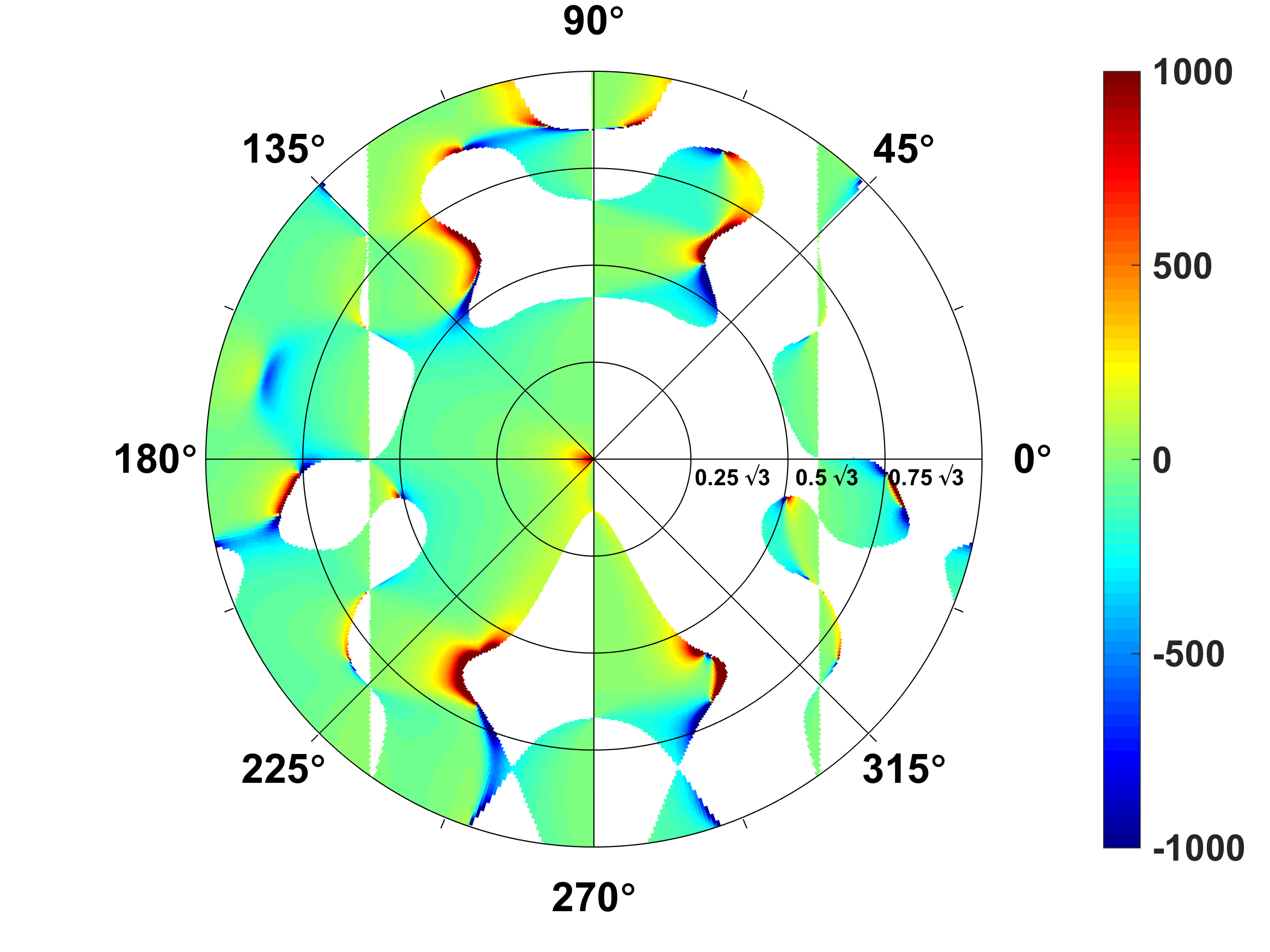
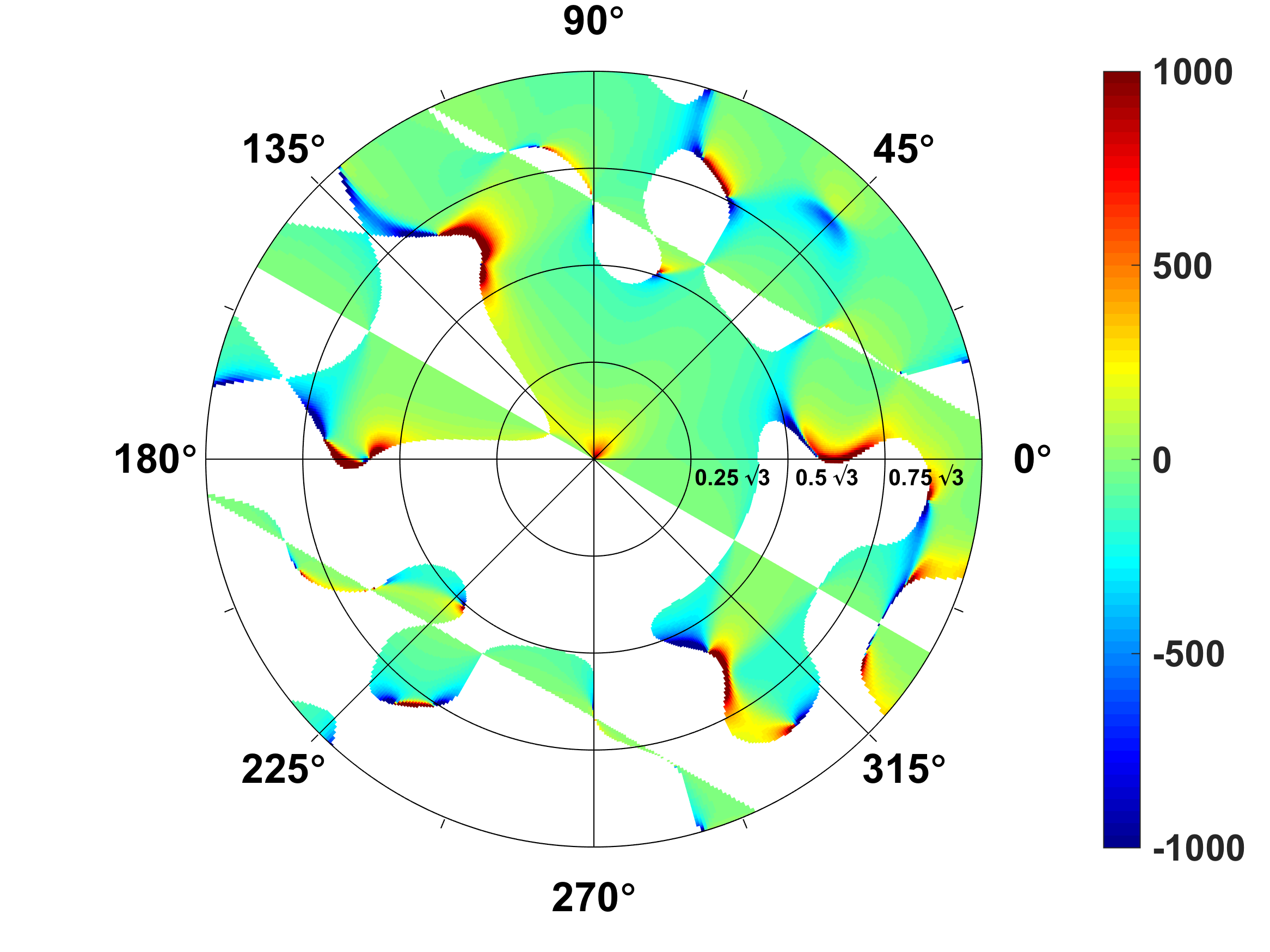
Figure 9: Real parts of the complex-valued impedance $\mu_{1}$ (left) and $\mu_{2}$ (right), in units of $a^{2}/D$, as functions of $d$ and $\theta_{d}$ for the incident wave $\theta_{0}=\pi/4$ and $k=\pi/(a\ \cos\theta_{0})$ (with $a=1$), for the $N=3$ triangular cluster negative refractor.

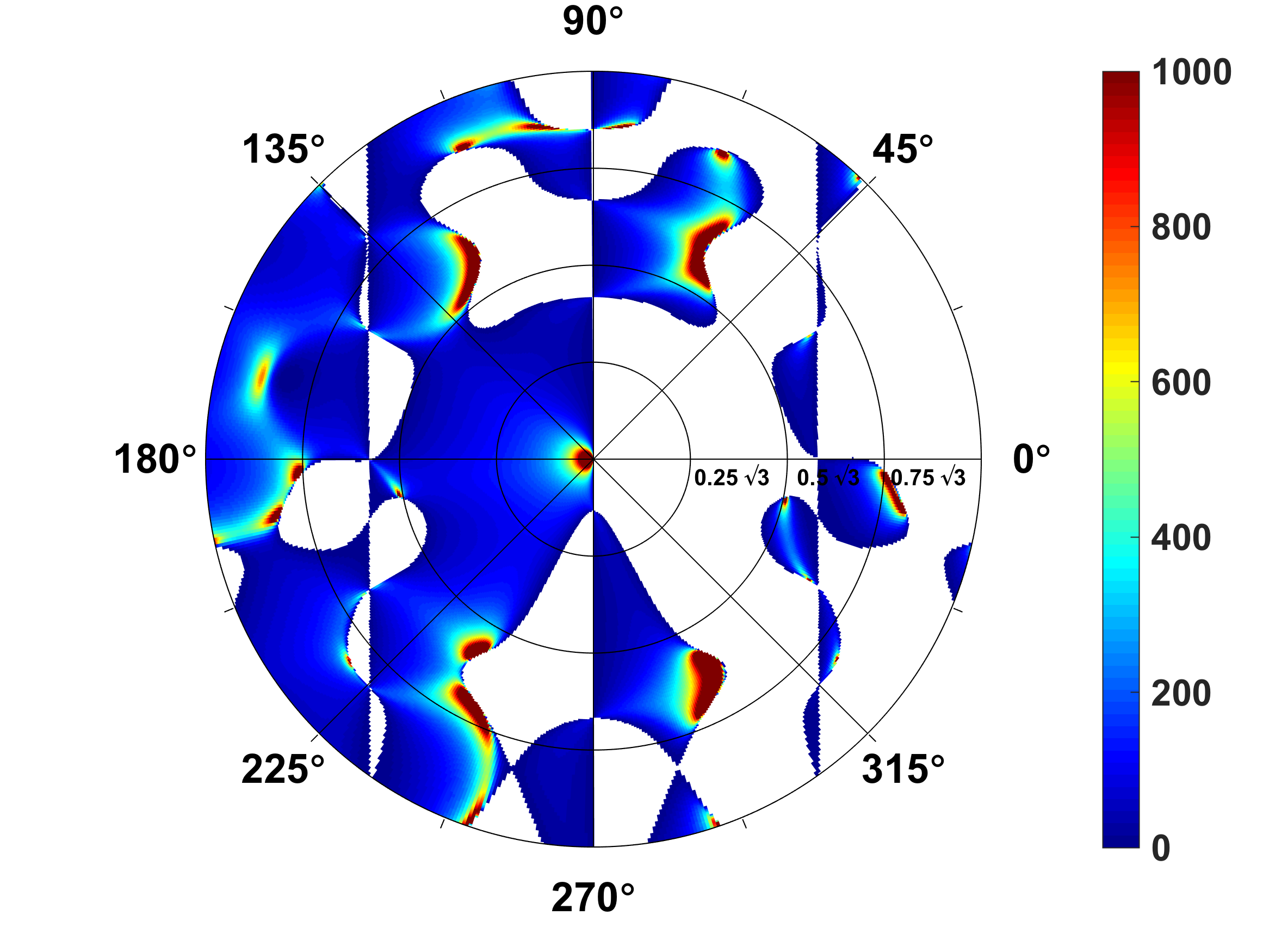
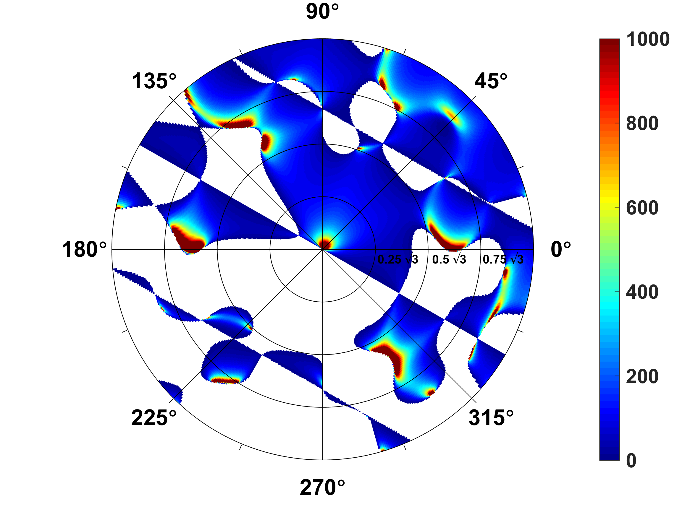
Figure 10: Imaginary parts of the impedance $\mu_{1}$ (left) and $\mu_{2}$ (right), in units of $a^{2}/D$, for the incident wave $\theta_{0}=\pi/4$, $k=\pi/(a\ \cos\theta_{0})$ (for $a=1$), for the $N=3$ triangular cluster negative refractor.

Combinations of $(d,\theta_{d})$, with the values of $|t_{-1}|$ satisfying $\operatorname{Im}\mu_{\alpha}>0$ for all $\alpha$, i.e. a passive cluster, are shown in Figure 11.

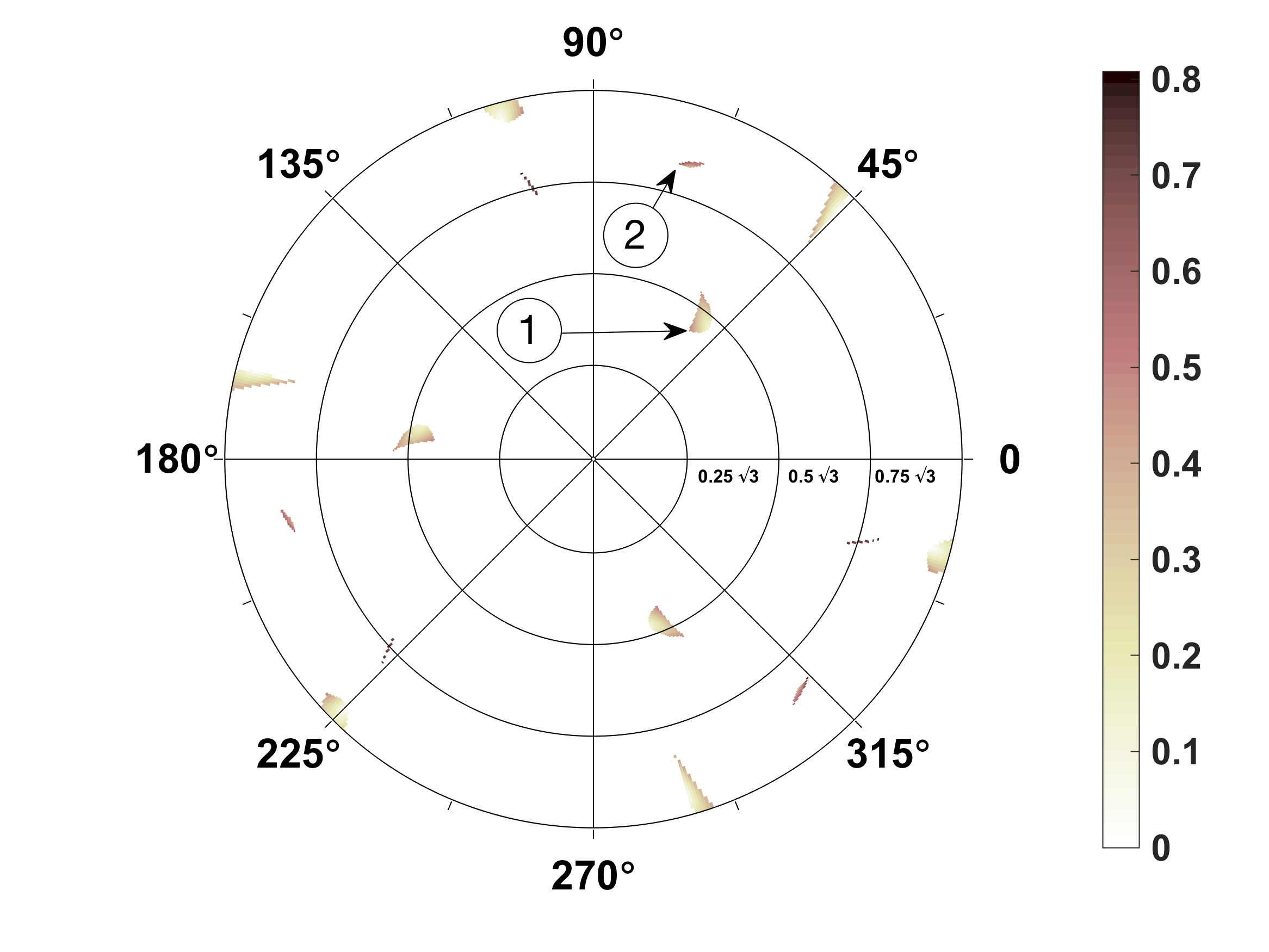
Figure 11: Transmission magnitude $|t_{-1}|$ of the designed triangular cluster negative refractor as a function of the scatterers’ radial, $d$, and angular, $\theta_{d}$, coordinates. The plotted regions correspond to passive $\mu_{\alpha}$ for all $\alpha$, and the labels are the selected clusters of table 1.

As for the linear cluster, we select $(d,\theta_{d})$ pairs with relatively large values of $|t_{-1}|$. For the triangular cluster these are $(0.7484,0.9237)$ and $(1.438,1.281)$, with impedances listed in table 1. Figures 12 and 13 show the reflection and transmission coefficients as a function of $k\times a$ for the chosen triangular clusters \raisebox{-.9pt} {1}⃝ and \raisebox{-.9pt} {2}⃝. The triangular cluster \raisebox{-.9pt} {1}⃝ displays moderate broadband response, while cluster \raisebox{-.9pt} {2}⃝ is narrowband, thus sensitive to the frequency of the incident wave.

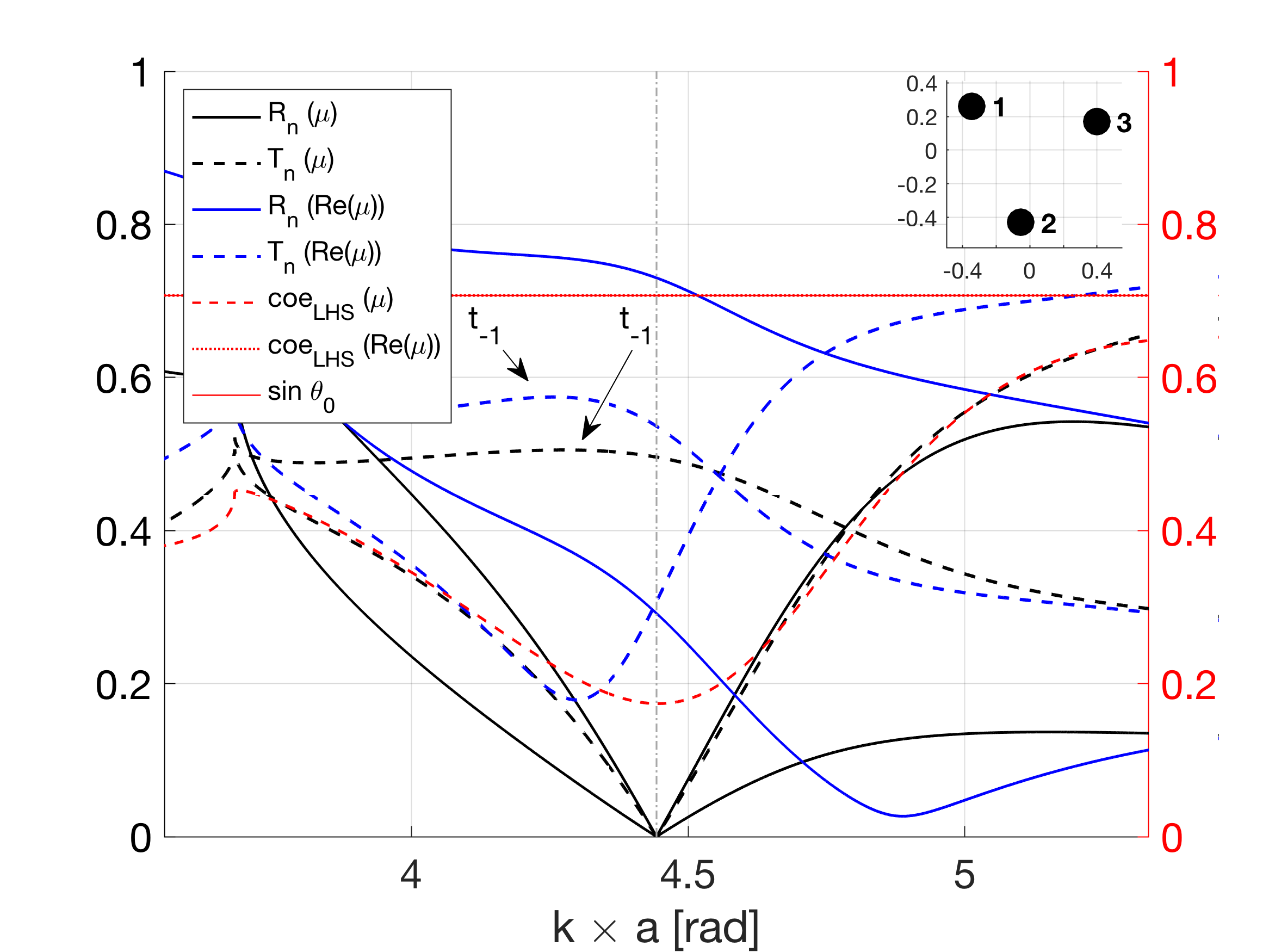
Figure 12: Reflection and transmission magnitudes for the triangular cluster ① defined in table 1 for complex values of $\mu_{\alpha}$ and for $\operatorname{Im}\mu_{\alpha}=0$. The vertical dash-dot line at $k\times a=\pi/\cos\pi/4$ indicates the operating frequency.

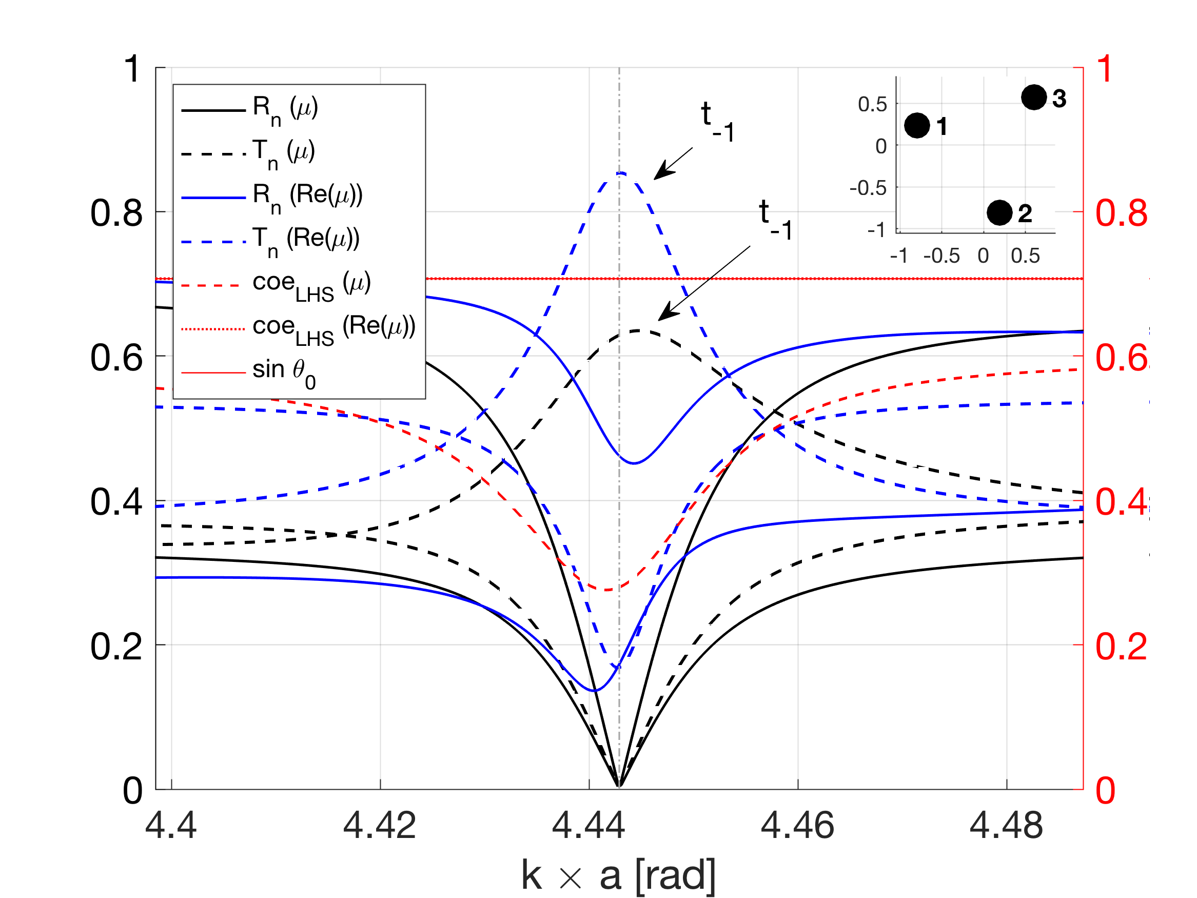
Figure 13: Reflection and transmission magnitudes for the triangular cluster ② with properties from table 1 for complex values of $\mu_{\alpha}$ and for $\operatorname{Im}\mu_{\alpha}=0$. The vertical dash-dot line at $k\times a=\pi/\cos\pi/4$ identifies the operational frequency of the grating.

Figures 12 and 13 also show the reflection and transmission characteristics for the triangular clusters \raisebox{-.9pt} {1}⃝ and \raisebox{-.9pt} {2}⃝, respectively, computed using only the real parts of the impedances, given in table 1. Setting the imaginary parts of the impedances to zero results in a significant drop in grating performance. The reflection and transmission coefficients that were zeroed out with the complex impedance now assume high values, exceeding the transmission coefficient of the $n=-1$ diffracted mode in all cases. This contrasts with the linear clusters for which the effect of setting $\operatorname{Im}\mu_{\alpha}=0$ is minimal, see Figures 7 and 8. The difference can be explained by the observation from table 1 that the impedances of the linear clusters are all lightly damped, while each of the triangular clusters has one impedance that is significantly damped.

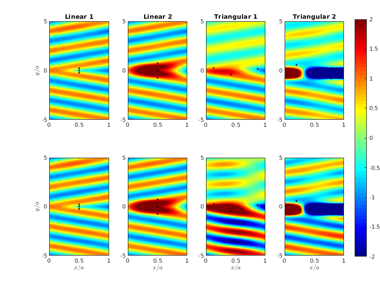
Figure 14: Field maps of the diffraction of a plane wave by the different clusters of resonators as defined in Table 1. Upper panels show the full solution and lower panels show the same cluster but setting ${\operatorname{Im}(\mu_{\alpha})=0}$. The black dots represent the point impedances within one period of the infinite grating.

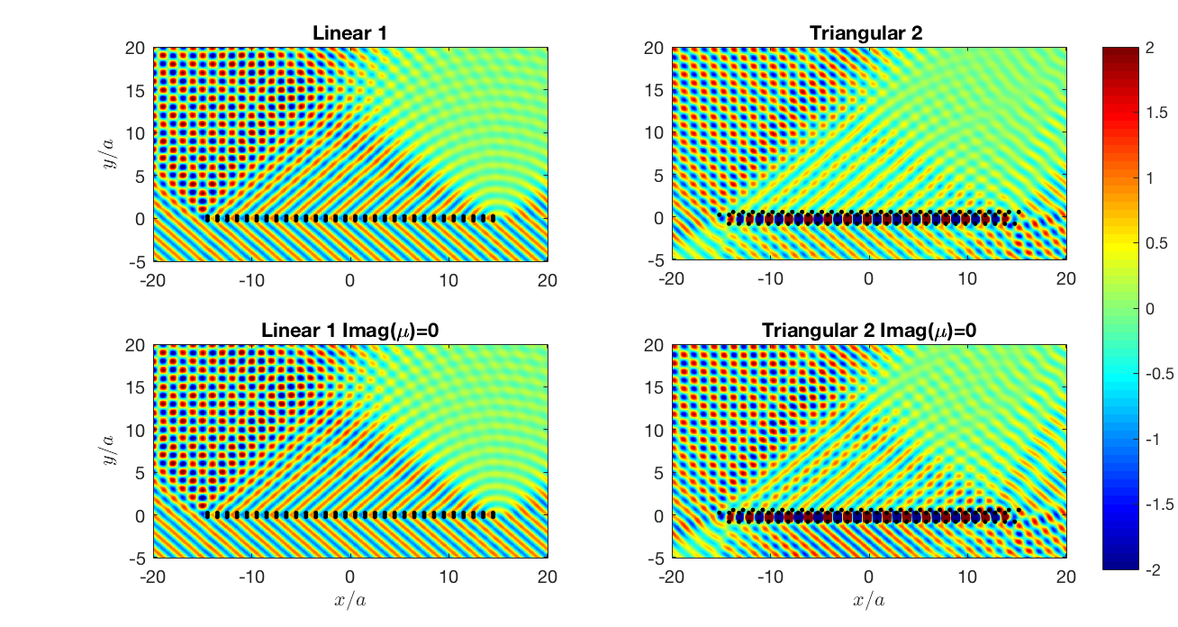
Figure 15: The total field amplitude for plane wave incidence on finite gratings of 30 clusters. The parameters are otherwise the same as in Figure 14 for the infinite grating.

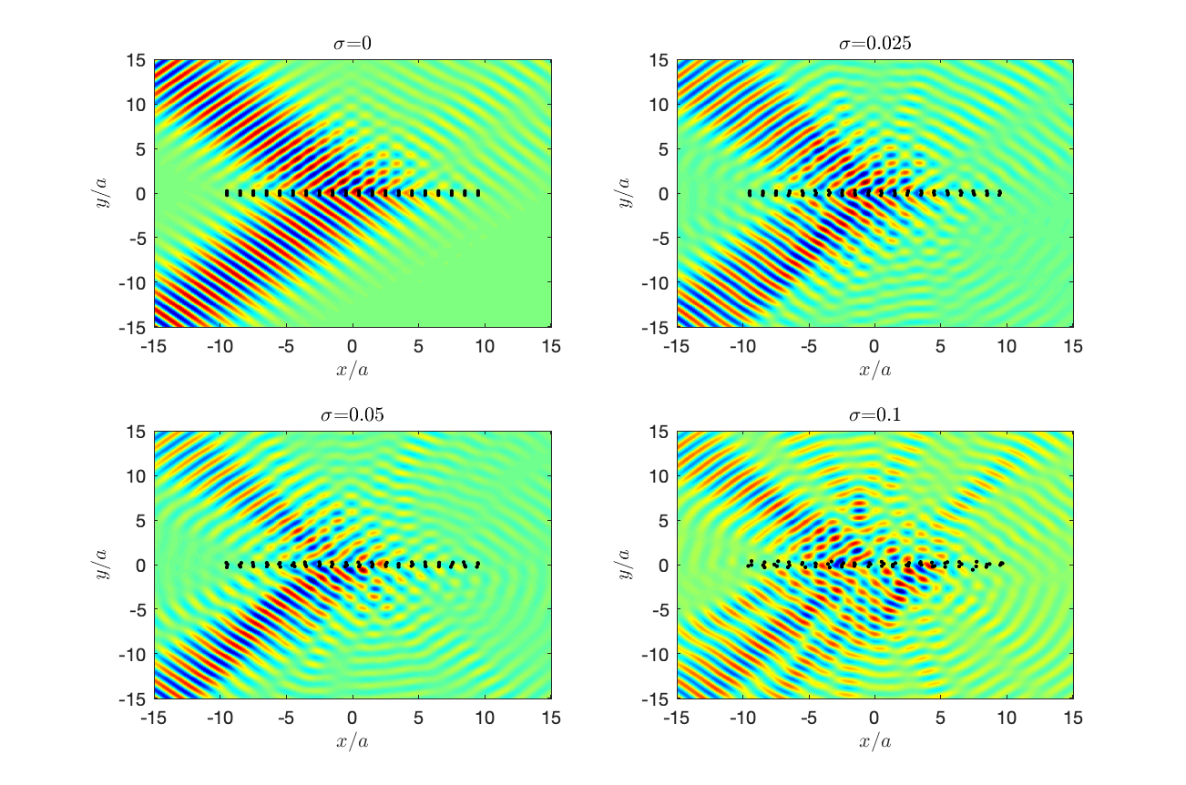
Figure 16: Multiple scattering simulations of finite gratings under Gaussian beam excitation. The parameter $\sigma$ represents the degree of random disorder that has been added to all the scatterers of the cluster.

IV.3.3 Infinite and finite retroreflector gratings with disorder

Figure 14 shows the field distributions for the designed $N=3$ gratings. The upper panels show the simulation of an incident plane wave from the negative $y$ direction with incident angle $\theta_{0}=\pi/4$ and wavenumber for the different configurations defined in Table 1. The lower panels show results for the same cluster after setting the imaginary part equal to zero. The negative refraction is evident in the simulations, and it is clear as well that, the larger the imaginary part of $\mu_{\alpha}$ the weaker the refracted wave. This is a consequence of the loss of wave energy caused by the highly damped resonators, although it is noted that the channeling of all the energy towards the $n=-1$ mode is still efficient in the sense that other modes are zeroed out, as designed. Overall, we see how ignoring the imaginary part has no visible effect in the linear cluster but drastically diminishes the amplitude of the refracted mode in the triangular clusters. As noted above, the reason for this may be understood from the fact that scatterers of the linear clusters are lightly damped but the triangular clusters have at least one highly damped impedance, see Table 1.

Finally, Figures 15 and 16 demonstrate that the effects predicted for the infinite grating are robust under finite limitations on the grating size, for finite incident beams, and in the presence of positional disorder. Thus, the same effects as observed for the infinite grating in Figure 14 are apparent in Figure 15 which shows the total field for incidence on a finite grating of 30 clusters of the linear and triangular configurations. The same finite configuration is considered in Figure 16 for Gaussian beam incidence, and for imperfections in the grating. The simulations indicate that good agreement with the infinite system under plane wave incidence is expected for zero and small levels of disorder.

V Practical considerations on scatterers and clusters

The grating performance, in terms of its reflection and transmission properties, depends on deviations of actual operation conditions from designed ones. Here we consider the performance as a function of deviations in scatterer positions, impedances, and the operating wavelength.

Anomalous refractors and reflectors are obviously narrowband, since the effect is due to diffraction which by definition is wavelength-dependent by (see equation (24)). However, this dependence is smooth, so that small deviations from the incident angle or desired wavelength produce small deviations in the diffracted angle. This is also true for the channeling of energy; as can be seen in Figures 7 and 8, the frequency dependence of the energy exchange between modes is smooth around the optimal value. Small variations about the optimal point produce small additional scattered waves, while the overall effect remains unchanged.

We have already seen in in Figures 7, 8, 12 and 13 how the reflection and transmission coefficients depend on changes in the incident wavenumber, for linear and triangular clusters respectively. Figures17 - 20 illustrate the influence of changes in scatterer positions (Figures 17 - 20) and impedances (real and imaginary parts, Figures 17 - 20) on reflection and transmission coefficients for the linear and triangular cluster.

These sensitivity studies show that dependence on the horizontal ($x$-)positions of the grating scatterers are negligible. They also indicate that linear clusters display small sensitivity to the positioning of the central scatterer. The first of linear clusters (\raisebox{-.9pt} {1}⃝), i.e. a linear configuration with small scatterers’ spacing, shows sensitivity measures related to position changes that are two orders smaller than for other clusters (linear \raisebox{-.9pt} {2}⃝ and triangular \raisebox{-.9pt} {1}⃝ and \raisebox{-.9pt} {2}⃝). The target transmitted mode coefficient, $t_{-1}$, is the least sensitive parameter to changes in scatterers’ positions (see figs. 17 - 20), meaning that grating performance will be rather affected by increase in other diffracted mode amplitudes, than decrease in the target mode amplitude, $t_{-1}$.

In general, it can be seen that for both cluster types, i.e. linear and triangular, small (negligible) variations in reflection/transmission coefficients are expected for small shifts of all scatterers’ positions, as shown in figs. 17 to 20. Also, provided impedance values given in tab. 1, relatively small impact of changes in impedances (real and imaginary parts) on reflection and transmission coefficients can be seen from figs. 17 - 20. Interestingly, for both cluster types, damping properties are critical to the grating performance. For the two linear clusters considered (\raisebox{-.9pt} {1}⃝ and \raisebox{-.9pt} {2}⃝) and the second configuration for the triangular cluster (\raisebox{-.9pt} {2}⃝), it is seen that damping - related to the imaginary part of impedance - has the highest influence on $t_{-1}$.

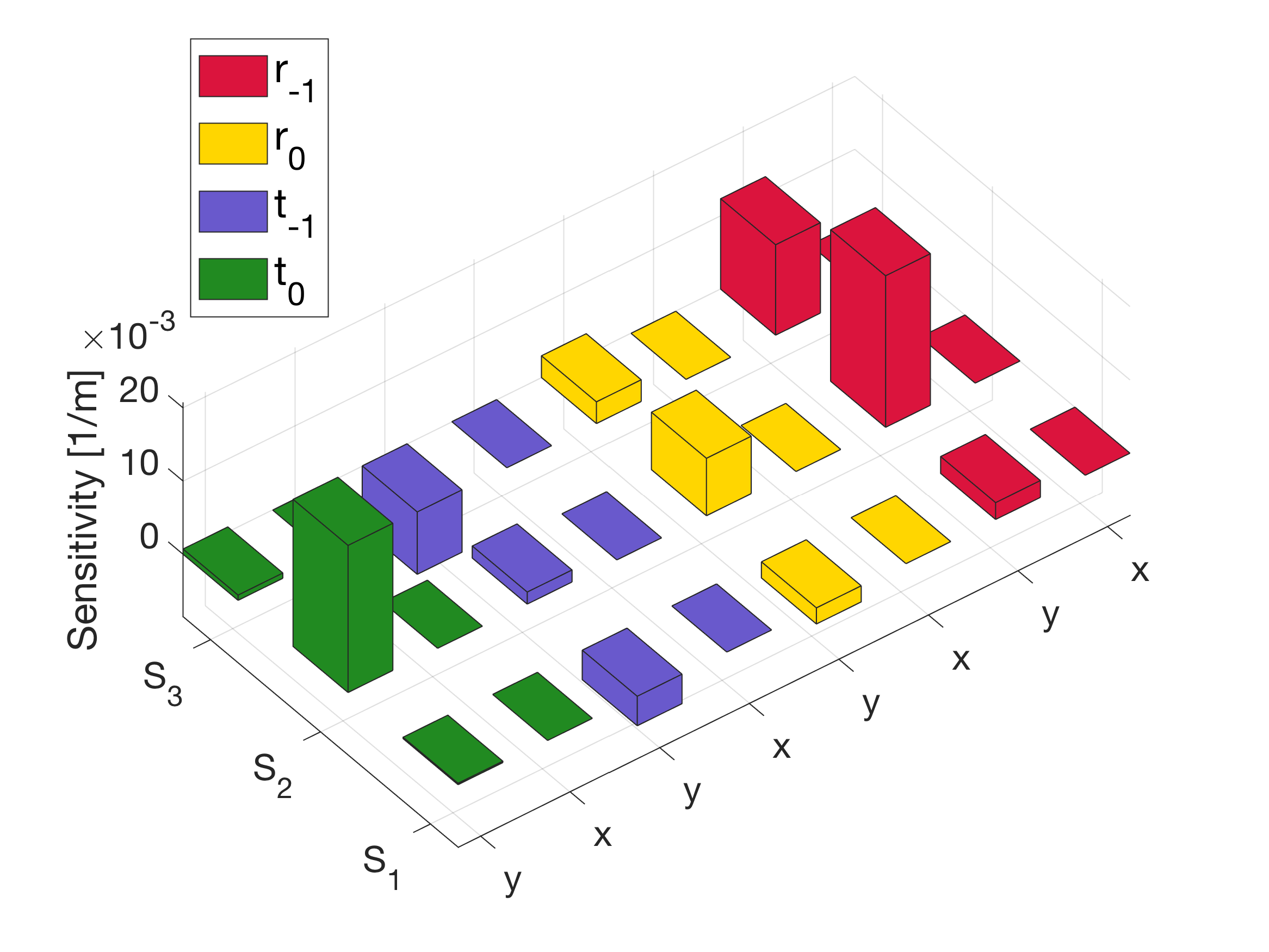
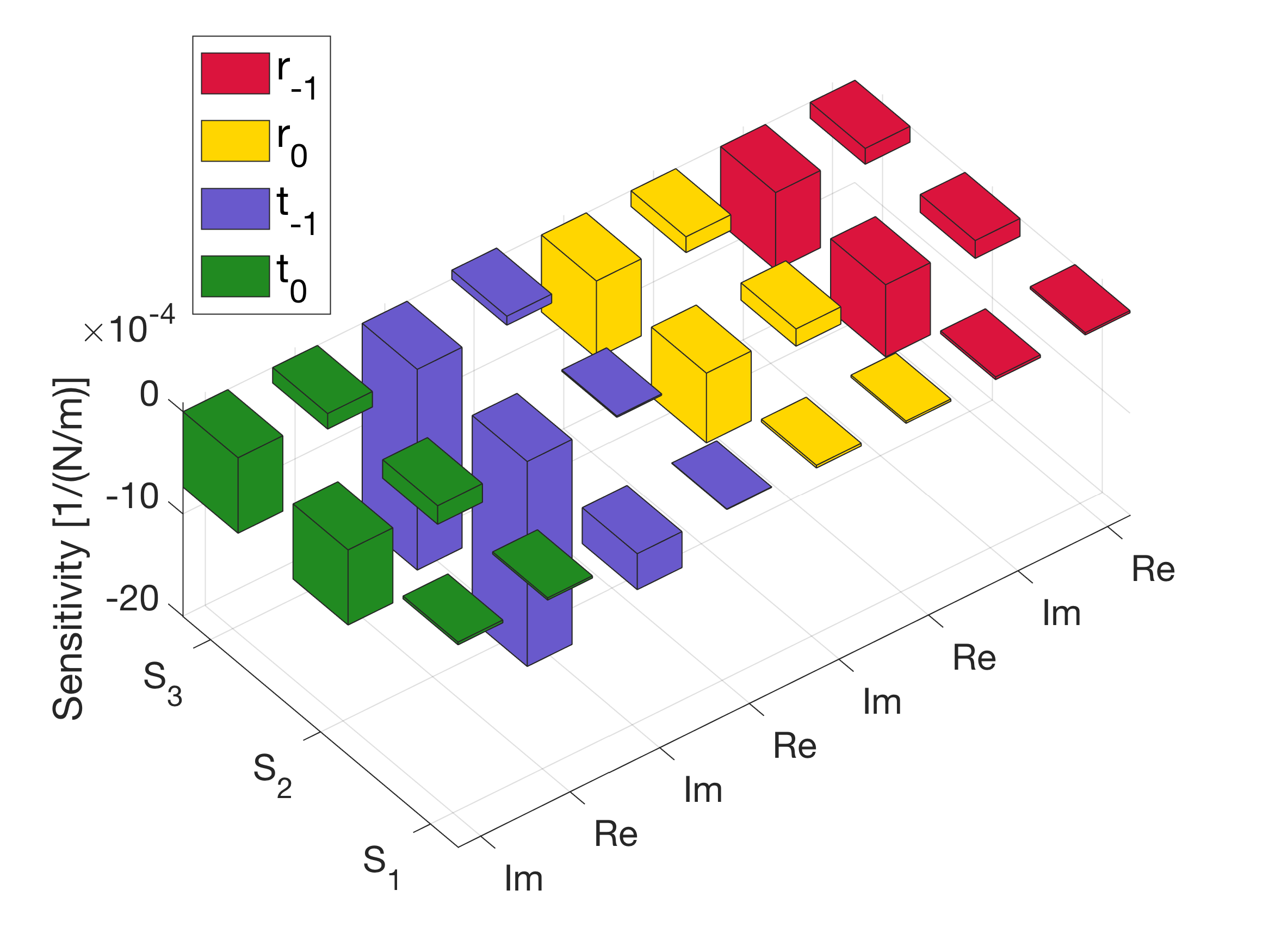
Figure 17: Sensitivity parameters for the linear ① cluster ($d=0.225$, $\theta_{d}=\pi/2$). (a) sensitivity parameters for individual changes in scatterers ($S_{1}$ - $S_{3}$) positions ($x$ and $y$) for the four diffracted modes reflection and transmission coefficients (for fixed $\mu$); (b) sensitivity parameters for individual changes in scatterers real and imaginary parts of impedances ($\mu_{1}$ - $\mu_{3}$) for the four diffracted modes reflection and transmission coefficients (fixed $S_{1}$ - $S_{3}$ positions).

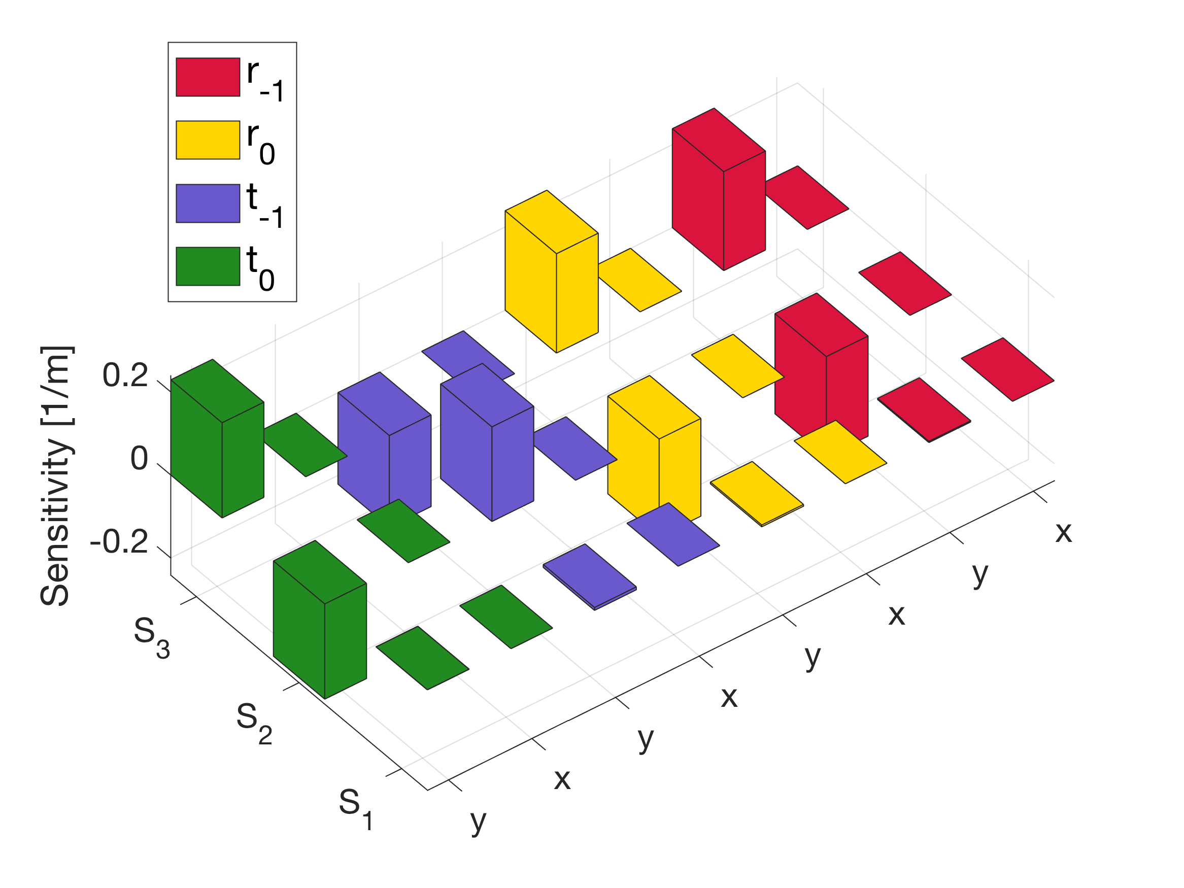
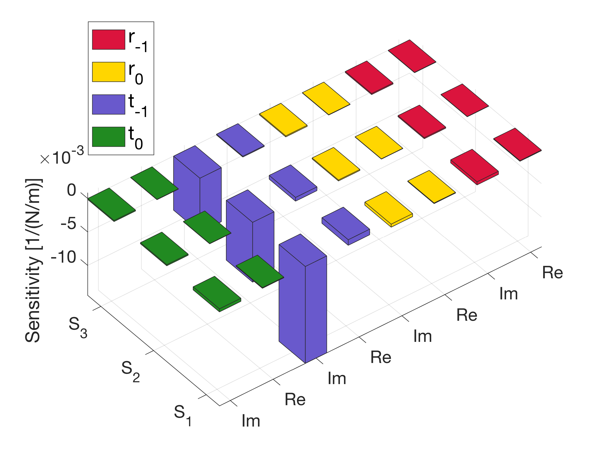
Figure 18: Sensitivity parameters for the linear ② cluster ($d=0.75$, $\theta_{d}=\pi/2$). (a) sensitivity parameters for individual changes in scatterers ($S_{1}$ - $S_{3}$) positions ($x$ and $y$) for the four diffracted modes reflection and transmission coefficients (for fixed $\mu$); (b) sensitivity parameters for individual changes in scatterers real and imaginary parts of impedances ($\mu_{1}$ - $\mu_{3}$) for the four diffracted modes reflection and transmission coefficients (fixed $S_{1}$ - $S_{3}$ positions).

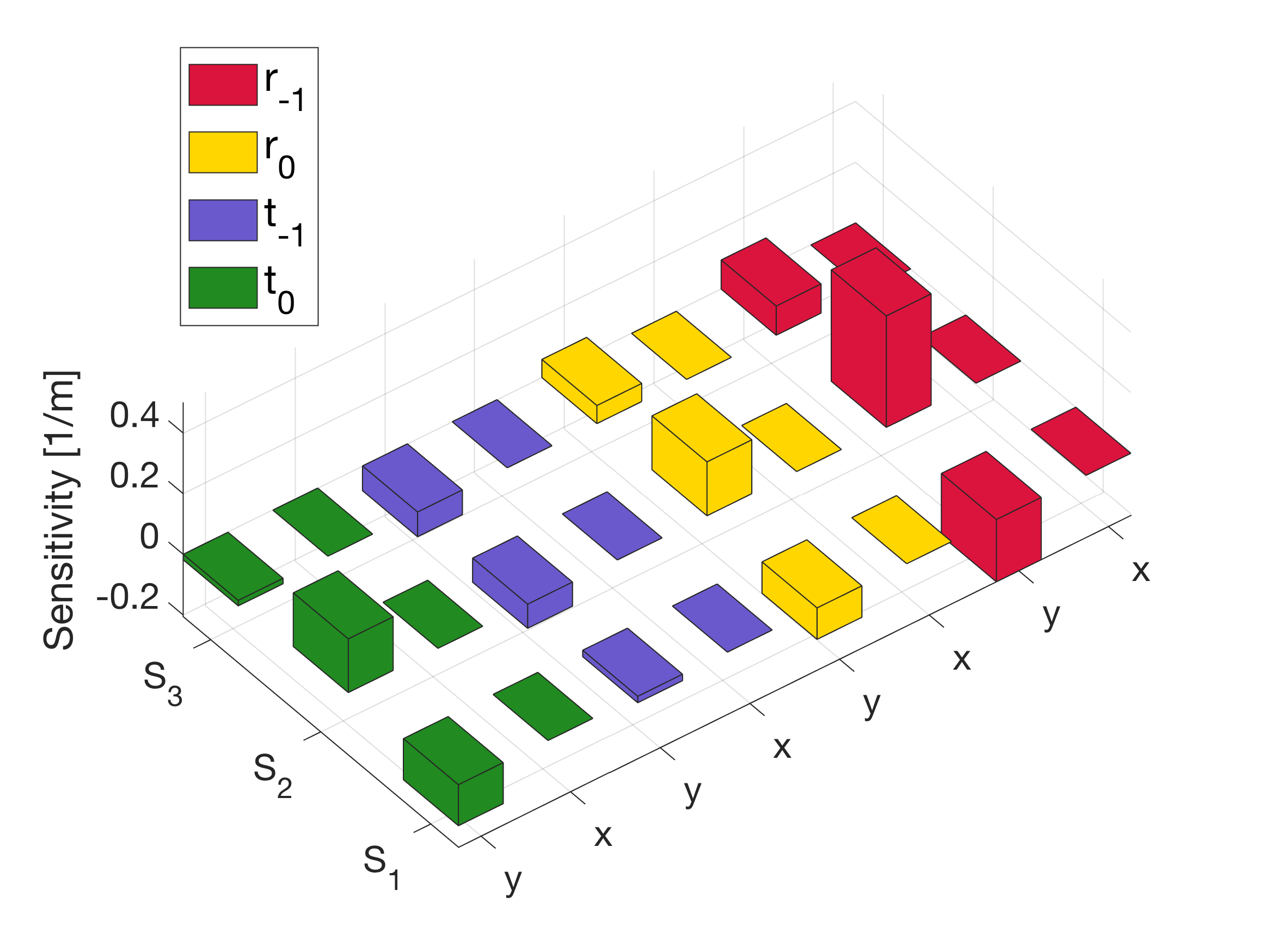
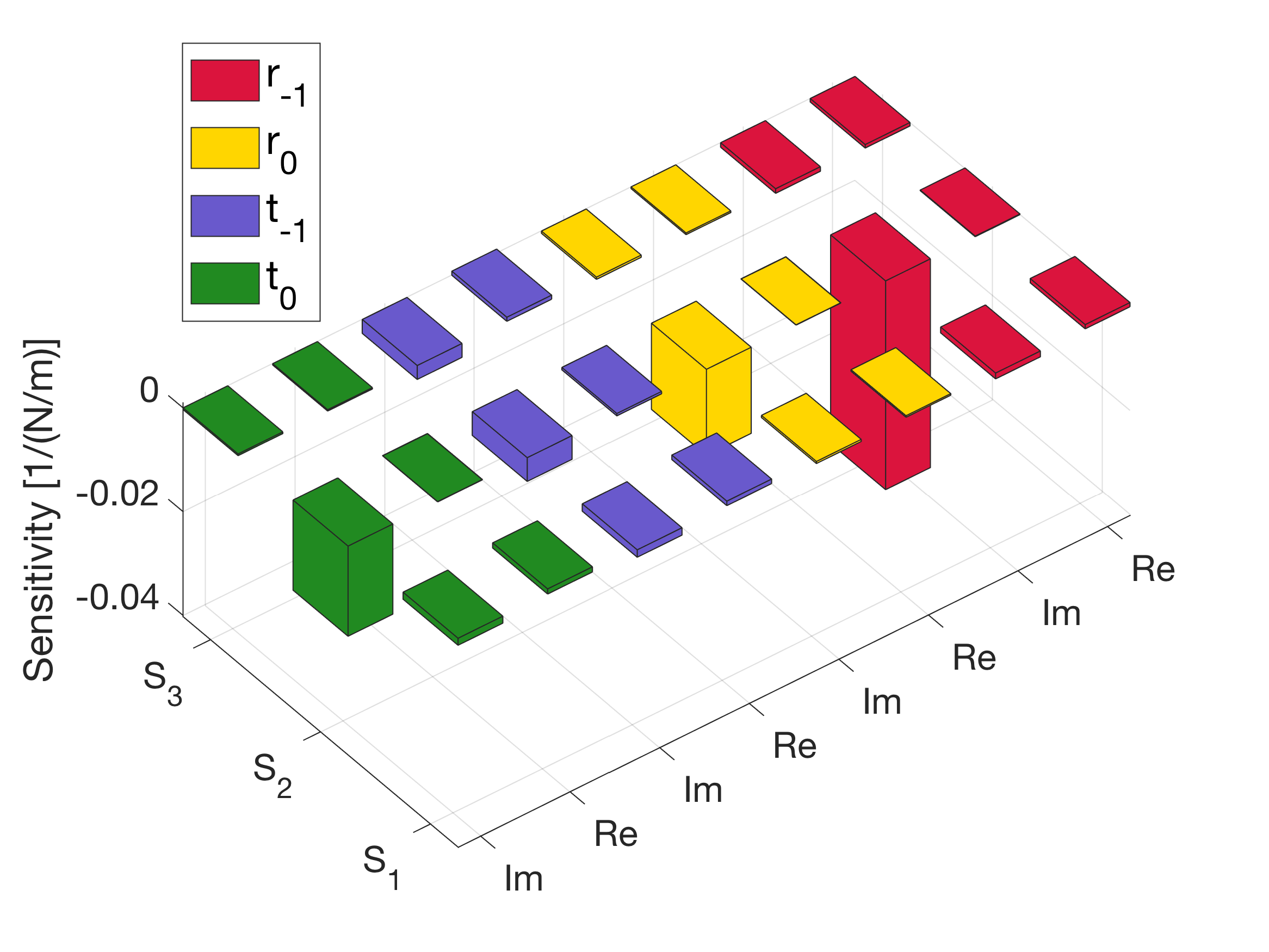
Figure 19: Sensitivity parameters for the triangular ① cluster ($d=0.75$, $\theta_{d}=0.92$). (a) sensitivity parameters for individual changes in scatterers ($S_{1}$ - $S_{3}$) positions ($x$ and $y$) for the four diffracted modes reflection and transmission coefficients (for fixed $\mu$); (b) sensitivity parameters for individual changes in scatterers real and imaginary parts of impedances ($\mu_{1}$ - $\mu_{3}$) for the four diffracted modes reflection and transmission coefficients (fixed $S_{1}$ - $S_{3}$ positions).

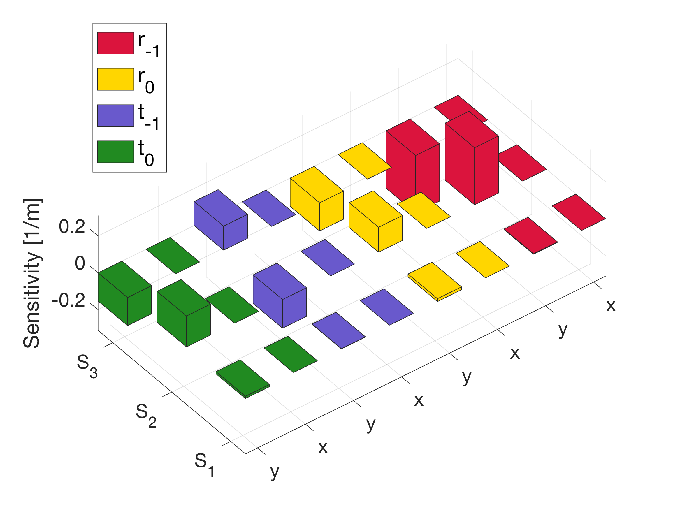
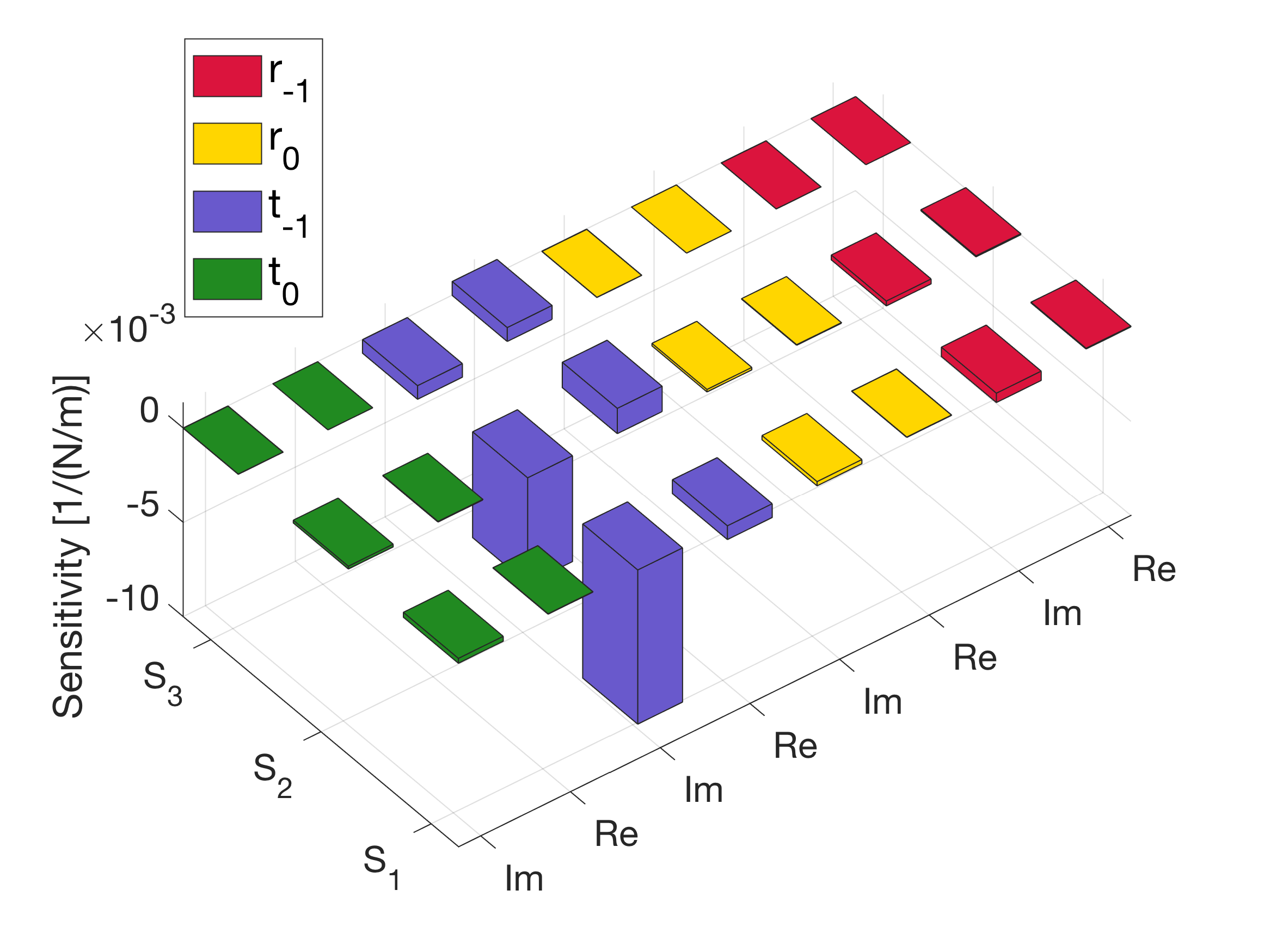
Figure 20: Sensitivity parameters for the triangular ② cluster ($d=0.75$, $\theta_{d}=0.92$). (a) sensitivity parameters for individual changes in scatterers ($S_{1}$ - $S_{3}$) positions ($x$ and $y$) for the four diffracted modes reflection and transmission coefficients (for fixed $\mu$); (b) sensitivity parameters for individual changes in scatterers real and imaginary parts of impedances ($\mu_{1}$ - $\mu_{3}$) for the four diffracted modes reflection and transmission coefficients (fixed $S_{1}$ - $S_{3}$ positions).

VI Summary

We have described a general approach for the inverse design of gratings for flexural waves in thin plates. Using a one-dimensional periodic arrangement of clusters of a finite number of point attachments it is possible to channel the incident energy towards a desired direction. The general solution for the inverse problem requires a cluster of both active and passive attachments, however it is possible to find solutions with only passive point scatterers. The required mechanical properties of the attached scatterers are defined by the impedances, which are obtained by solving a linear system of equations. We have shown through specific examples that some configurations, the linear clusters, possess very low dissipation, resulting in very high conversion to the desired refracted mode. It should be noted that the impedances of the cluster elements are linearly related to the desired diffraction parameters; the design process requires only a matrix inversion. It has to be pointed out that the present approach, although derived for flexural waves and for the specific example of the negative refractor, can be easily exported to other waves and devices.

Appendix A Plate Green’s function

The Green’s function, which satisfies

$$D\big{(}\Delta^{2}G({\bf r})-k^{4}G({\bf r})\big{)}=\delta({\bf r}),$$ (48)

can be readily obtained using a double Fourier transform as

$$G({\bf r})=\frac{1}{D(2\pi)^{2}}\int_{{\mathbb{R}}^{2}}\frac{e^{\mathrm{i}(\xi x+\eta y)}\operatorname{d}\xi\operatorname{d}\eta}{(\xi^{2}+\eta^{2})^{2}-k^{4}}.$$ (49)

Evaluating the $\eta$ integral using the Cauchy residue theorem gives

$$G({\bf r}) =\frac{1}{2\pi}\int_{{\mathbb{R}}}\operatorname{d}\xi\,e^{\mathrm{i}\xi x}f(\xi,y),$$ (50a)

$$f(\xi,y) =\frac{1}{4Dk^{2}}\bigg{(}\frac{e^{-(\xi^{2}-k^{2})^{1/2}|y|}}{(\xi^{2}-k^{2})^{1/2}}-\frac{e^{-(\xi^{2}+k^{2})^{1/2}|y|}}{(\xi^{2}+k^{2})^{1/2}}\bigg{)}.$$ (50b)

Note that $(\xi^{2}-k^{2})^{1/2}=-\mathrm{i}\sqrt{k^{2}-\xi^{2}}$ for $|\xi|<k$. The explicit form (6) follows using known integral representations for the Hankel function.

The line sum

$$\sum_{m\in\mathbb{Z}}e^{\mathrm{i}k_{x}ma}\,G({\bf r}-ma\hat{\bf x})=\sum_{m\in\mathbb{Z}}\frac{1}{2\pi}\int_{{\mathbb{R}}}\operatorname{d}\xi\,e^{\mathrm{i}ma(k_{x}-\xi)}\,e^{\mathrm{i}\xi x}f(\xi,y)$$ (51)

can be simplified using the Poisson summation formula

$$\sum_{m\in\mathbb{Z}}\frac{1}{2\pi}\int_{{\mathbb{R}}}\operatorname{d}u\,e^{\pm\mathrm{i}mu}F(u)=\sum_{n\in\mathbb{Z}}F(2\pi n).$$ (52)

Hence,

$$\sum_{m\in\mathbb{Z}}e^{\mathrm{i}k_{x}ma}G({\bf r}-ma\hat{\bf x})=\frac{1}{a}\sum_{n\in\mathbb{Z}}e^{\mathrm{i}(k_{x}+\frac{2\pi}{a}n)x}f(k_{x}+\frac{2\pi}{a}n,y)$$ (53)

with $f$ defined in (50b). This gives the identity (19).

Appendix B The $N=3$ retroreflector grating, linear cluster

Assuming a configuration of $N=3$ scatterers, and using the fact that ${\bf k}_{-1}^{\pm}=-{\bf k}_{0}^{\mp}$ for the negative refractor, (47) becomes

$$\hat{\bf S}=\frac{\mathrm{i}G_{0}}{k\sin\theta_{0}}\begin{pmatrix}1&e^{-\mathrm{i}{\bf k}_{0}^{+}\cdot{\bf R}_{2}}&e^{-\mathrm{i}{\bf k}_{0}^{+}\cdot{\bf R}_{3}}\\ 1&e^{-\mathrm{i}{\bf k}_{0}^{-}\cdot{\bf R}_{2}}&e^{-\mathrm{i}{\bf k}_{0}^{-}\cdot{\bf R}_{3}}\\ 1&e^{\mathrm{i}{\bf k}_{0}^{+}\cdot{\bf R}_{2}}&e^{\mathrm{i}{\bf k}_{0}^{+}\cdot{\bf R}_{3}}\end{pmatrix},$$ (54)

Taking ${\bf R}_{2}=\bm{R}_{+}$, ${\bf R}_{3}=\bm{R}_{-}$, where $\bm{R}_{\pm}=\pm d(\cos\theta_{d},\sin\theta_{d})$, we have

$$\hat{\bf S}=\frac{\mathrm{i}G_{0}}{k\sin\theta_{0}}\begin{pmatrix}1&e^{-i\phi_{-}}&e^{i\phi_{-}}\\ 1&e^{-i\phi_{+}}&e^{i\phi_{+}}\\ 1&e^{i\phi_{-}}&e^{-i\phi_{-}}\\ \end{pmatrix}$$ (55)

where $\phi_{\pm}=kd\cos(\theta_{d}\pm\theta_{0})$. Note that

$$\det\hat{\bf S} =\frac{4G_{0}^{3}}{(k\sin\theta_{0})^{3}}\big{(}\cos\phi_{-}-\cos\phi_{+}\big{)}\sin\phi_{-}$$

$$=-\Big{(}\frac{2G_{0}}{k\sin\theta_{0}}\Big{)}^{3}\sin\big{(}kd\cos(\theta_{d}-\theta_{0})\big{)}\,\sin\big{(}kd\cos\theta_{d}\cos\theta_{0}\big{)}\,\sin\big{(}kd\sin\theta_{d}\sin\theta_{0}\big{)}$$ (56)

which clearly vanishes at the ”forbidden” values $\theta_{d}=0$, $\frac{\pi}{2}$ and $\pi$. However, referring to (41),

$$\hat{\bf S}^{-1}{\bf e}_{1}=\frac{k\sin\theta_{0}}{4\mathrm{i}G_{0}\sin\phi_{-}\sin\frac{1}{2}(\phi_{+}-\phi_{-})}\begin{pmatrix}-2\cos\frac{1}{2}(\phi_{+}+\phi_{-})\\ e^{{\mathrm{i}}(\phi_{+}-\phi_{-})/2}\\ e^{{\mathrm{i}}(\phi_{-}-\phi_{+})/2}\end{pmatrix}$$ (57)

which is well defined for $\theta_{d}=\frac{\pi}{2}$ even though $\det\hat{\bf S}=0$ at that angle.

References

- Ra’di et al. (2017) Younes Ra’di, Dimitrios L Sounas, and Andrea Alu, “Metagratings: Beyond the limits of graded metasurfaces for wave front control,” Physical Review Letters 119, 067404 (2017).
- Epstein and Rabinovich (2017) Ariel Epstein and Oshri Rabinovich, “Unveiling the properties of metagratings via a detailed analytical model for synthesis and analysis,” Physical Review Applied 8, 054037 (2017).
- Wong and Eleftheriades (2018) Alex MH Wong and George V Eleftheriades, “Perfect anomalous reflection with a bipartite Huygens’ metasurface,” Physical Review X 8, 011036 (2018).
- Quan et al. (2018) Li Quan, Younes Ra’di, Dimitrios L Sounas, and Andrea Alù, “Maximum Willis coupling in acoustic scatterers,” Physical Review Letters 120, 254301 (2018).
- Rabinovich and Epstein (2018) Oshri Rabinovich and Ariel Epstein, “Analytical design of printed-circuit-board (pcb) metagratings for perfect anomalous reflection,” arXiv preprint arXiv:1801.04521 (2018).
- Epstein and Rabinovich (2018) Ariel Epstein and Oshri Rabinovich, “Perfect anomalous refraction with metagratings,” arXiv preprint arXiv:1804.02362 (2018).
- Yu et al. (2011) Nanfang Yu, Patrice Genevet, Mikhail A Kats, Francesco Aieta, Jean-Philippe Tetienne, Federico Capasso, and Zeno Gaburro, “Light propagation with phase discontinuities: generalized laws of reflection and refraction,” Science 334, 333–337 (2011).
- Torrent (2018) Daniel Torrent, “Acoustic anomalous reflectors based on diffraction grating engineering,” Phys. Rev. B 98, 060101 (2018).
- Evans and Porter (2007) D. V. Evans and R. Porter, “Penetration of flexural waves through a periodically constrained thin elastic plate in vacuo and floating on water,” Journal of Engineering Mathematics 58, 317–337 (2007).
- Xiao et al. (2012) Yong Xiao, Jihong Wen, and Xisen Wen, “Flexural wave band gaps in locally resonant thin plates with periodically attached spring–mass resonators,” Journal of Physics D: Applied Physics 45, 195401 (2012).
- Torrent et al. (2013) Daniel Torrent, Didier Mayou, and José Sánchez-Dehesa, “Elastic analog of graphene: Dirac cones and edge states for flexural waves in thin plates,” Physical Review B 87 (2013), 10.1103/physrevb.87.115143.
- Pal and Ruzzene (2017) Raj Kumar Pal and Massimo Ruzzene, “Edge waves in plates with resonators: an elastic analogue of the quantum valley hall effect,” New Journal of Physics 19, 025001 (2017).
- Movchan et al. (2009) N. V. Movchan, R. C. McPhedran, A. B. Movchan, and C. G. Poulton, “Wave scattering by platonic grating stacks,” Proceedings of the Royal Society A: Mathematical, Physical and Engineering Sciences 465, 3383–3400 (2009).
- Haslinger et al. (2011) S. G. Haslinger, N. V. Movchan, A. B. Movchan, and R. C. McPhedran, “Transmission, trapping and filtering of waves in periodically constrained elastic plates,” Proceedings of the Royal Society A: Mathematical, Physical and Engineering Sciences 468, 76–93 (2011).
- Haslinger et al. (2017) S. G. Haslinger, N. V. Movchan, A. B. Movchan, I. S. Jones, and R. V. Craster, “Controlling flexural waves in semi-infinite platonic crystals with resonator-type scatterers,” The Quarterly Journal of Mechanics and Applied Mathematics 70, 216–247 (2017).
- Gusev and Wright (2014) Vitalyi E Gusev and Oliver B Wright, “Double-negative flexural acoustic metamaterial,” New Journal of Physics 16, 123053 (2014).
- Torrent et al. (2014) Daniel Torrent, Yan Pennec, and Bahram Djafari-Rouhani, “Effective medium theory for elastic metamaterials in thin elastic plates,” Physical Review B 90 (2014), 10.1103/physrevb.90.104110.
- Farhat et al. (2010) M. Farhat, S. Guenneau, and S. Enoch, “High directivity and confinement of flexural waves through ultra-refraction in thin perforated plates,” EPL (Europhysics Letters) 91, 54003 (2010).
- Smith et al. (2012) Michael J.A. Smith, Ross C. McPhedran, Chris G. Poulton, and Michael H. Meylan, “Negative refraction and dispersion phenomena in platonic clusters,” Waves in Random and Complex Media 22, 435–458 (2012).
- Meylan and McPhedran (2011) M. H. Meylan and R. C. McPhedran, “Fast and slow interaction of elastic waves with platonic clusters,” Proceedings of the Royal Society A: Mathematical, Physical and Engineering Sciences 467, 3509–3529 (2011).
- Movchan et al. (2007) A.B. Movchan, N.V. Movchan, and R.C. McPhedran, “Bloch–floquet bending waves in perforated thin plates,” Proceedings of the Royal Society A: Mathematical, Physical and Engineering Sciences 463, 2505–2518 (2007).
- Brennan (1997) MJ Brennan, “Vibration control using a tunable vibration neutralizer,” Proceedings of the Institution of Mechanical Engineers, Part C: Journal of Mechanical Engineering Science 211, 91–108 (1997).
- Brennan (1999) MJ Brennan, “Control of flexural waves on a beam using a tunable vibration neutraliser,” Journal of Sound and Vibration 222, 389–407 (1999).
- El-Khatib et al. (2005) HM El-Khatib, BR Mace, and MJ Brennan, “Suppression of bending waves in a beam using a tuned vibration absorber,” Journal of Sound and Vibration 288, 1157–1175 (2005).