Causal Explanation Analysis on Social Media

Abstract

Understanding causal explanations — reasons given for happenings in one’s life — has been found to be an important psychological factor linked to physical and mental health. Causal explanations are often studied through manual identification of phrases over limited samples of personal writing. Automatic identification of causal explanations in social media, while challenging in relying on contextual and sequential cues, offers a larger-scale alternative to expensive manual ratings and opens the door for new applications (e.g. studying prevailing beliefs about causes, such as climate change). Here, we explore automating causal explanation analysis, building on discourse parsing, and presenting two novel subtasks: causality detection (determining whether a causal explanation exists at all) and causal explanation identification (identifying the specific phrase that is the explanation). We achieve strong accuracies for both tasks but find different approaches best: an SVM for causality prediction ($F1=0.791$) and a hierarchy of Bidirectional LSTMs for causal explanation identification ($F1=0.853$). Finally, we explore applications of our complete pipeline ($F1=0.868$), showing demographic differences in mentions of causal explanation and that the association between a word and sentiment can change when it is used within a causal explanation.

1 Introduction

Explanations of happenings in one’s life, causal explanations, are an important topic of study in social, psychological, economic, and behavioral sciences. For example, psychologists have analyzed people’s causal explanatory style Peterson et al. (1988) and found strong negative relationships with depression, passivity, and hostility, as well as positive relationships with life satisfaction, quality of life, and length of life Scheier et al. (1989); Carver and Gaines (1987); Peterson et al. (1988).

Figure 1: A casual relation characterizes the connection between two discourse arguments, one of which is the causal explanation.

To help understand the significance of causal explanations, consider how they are applied to measuring optimism (and its converse, pessimism) Peterson et al. (1988). For example, in “My parser failed because I always have bugs.”, the emphasized text span is considered a causal explanation which indicates pessimistic personality – a negative event where the author believes the cause is pervasive. However, in “My parser failed because I barely worked on the code.”, the explanation would be considered a signal of optimistic personality – a negative event for which the cause is believed to be short-lived.

Language-based models which can detect causal explanations from everyday social media language can be used for more than automating optimism detection. Language-based assessments would enable other large-scale downstream tasks: tracking prevailing causal beliefs (e.g., about climate change or autism), better extracting process knowledge from non-fiction (e.g., gravity causes objects to move toward one another), or detecting attribution of blame or praise in product or service reviews (“I loved this restaurant because the fish was cooked to perfection”).

In this paper, we introduce causal explanation analysis and its subtasks of detecting the presence of causality (causality prediction) and identifying explanatory phrases (causal explanation identification). There are many challenges to achieving these task. First, the ungrammatical texts in social media incur poor syntactic parsing results which drastically affect the performance of discourse relation parsing pipelines . Many causal relations are implicit and do not contain any discourse markers (e.g., ‘because’). Further, Explicit causal relations are also more difficult in social media due to the abundance of abbreviations and variations of discourse connectives (e.g., ‘cuz’ and ‘bcuz’).

Prevailing approaches for social media analyses, utilizing traditional linear models or bag of words models (e.g., SVM trained with n-gram, part-of-speech (POS) tags, or lexicon-based features) alone do not seem appropriate for this task since they simply cannot segment the text into meaningful discourse units or discourse arguments such as clauses or sentences rather than random consecutive token sequences or specific word tokens. Even when the discourse units are clear, parsers may still fail to accurately identify discourse relations since the content of social media is quite different than that of newswire which is typically used for discourse parsing.

In order to overcome these difficulties of discourse relation parsing in social media, we simplify and minimize the use of syntactic parsing results and capture relations between discourse arguments, and investigate the use of a recursive neural network model (RNN). Recent work has shown that RNNs are effective for utilizing discourse structures for their downstream tasks Ji and Smith (2017); Bhatia et al. (2015); Wieting et al. (2015); Paulus et al. (2014), but they have yet to be directly used for discourse relation prediction in social media. We evaluated our model by comparing it to off-the-shelf end-to-end discourse relation parsers and traditional models. We found that the SVM and random forest classifiers work better than the LSTM classifier for the causality detection, while the LSTM classifier outperforms other models for identifying causal explanation.

The contributions of this work include: (1) the proposal of models for both (a) causality prediction and (b) causal explanation identification, (2) the extensive evaluation of a variety of models from social media classification models and discourse relation parsers to RNN-based application models, demonstrating that feature-based models work best for causality prediction while RNNs are superior for the more difficult task of causal explanation identification, (3) performance analysis on architectural differences of the pipeline and the classifier structures, (4) exploration of the applications of causal explanation to downstream tasks, and (5) release of a novel, anonymized causality Facebook dataset along with our causality prediction and causal explanation identification models.

2 Related Work

Identifying causal explanations in documents can be viewed as discourse relation parsing. The Penn Discourse Treebank (PDTB) Prasad et al. (2007) has a ‘Cause’ and ‘Pragmatic Cause’ discourse type under a general ‘Contingency’ class and Rhetorical Structure Theory (RST) Mann and Thompson (1987) has a ‘Relations of Cause’. In most cases, the development of discourse parsers has taken place in-domain, where researchers have used the existing annotations of discourse arguments in newswire text (e.g. Wall Street Journal) from the discourse treebank and focused on exploring different features and optimizing various types of models for predicting relations Pitler et al. (2009); Park and Cardie (2012); Zhou et al. (2010). In order to further develop automated systems, researchers have proposed end-to-end discourse relation parsers, building models which are trained and evaluated on the annotated PDTB and RST Discourse Treebank (RST DT). These corpora consist of documents from Wall Street Journal (WSJ) which are much more well-organized and grammatical than social media texts Biran and McKeown (2015); Lin et al. (2014); Ji and Eisenstein (2014); Feng and Hirst (2014).

Only a few works have attempted to parse discourse relations for out-of-domain problems such as text categorizations on social media texts; Ji and Bhatia used models which are pretrained with RST DT for building discourse structures from movie reviews, and Son adapted the PDTB discourse relation parsing approach for capturing counterfactual conditionals from tweets Bhatia et al. (2015); Ji and Smith (2017); Son et al. (2017). These works had substantial differences to what propose in this paper. First, Ji and Bhatia used a pretrained model (not fully optimal for some parts of the given task) in their pipeline; Ji’s model performed worse than the baseline on the categorization of legislative bills, which is thought to be due to legislative discourse structures differing from those of the training set (WSJ corpus). Bhatia also used a pretrained model finding that utilizing discourse relation features did not boost accuracy Bhatia et al. (2015); Ji and Smith (2017). Both Bhatia and Son used manual schemes which may limit the coverage of certain types of positive samples– Bhatia used a hand-crafted schema for weighting discourse structures for the neural network model and Son manually developed seven surface forms of counterfactual thinking for the rule-based system Bhatia et al. (2015); Son et al. (2017). We use social-media-specific features from pretrained models which are directly trained on tweets and we avoid any hand-crafted rules except for those included in the existing discourse argument extraction techniques.

The automated systems for discourse relation parsing involve multiple subtasks from segmenting the whole text into discourse arguments to classifying discourse relations between the arguments. Past research has found that different types of models and features yield varying performance for each subtask. Some have optimized models for discourse relation classification (i.e. given a document indicating if the relation existing) without discourse argument parsing using models such as Naive-Bayes or SVMs, achieve relatively stronger accuracies but a simpler task than that associated with discourse arguments Park and Cardie (2012); Zhou et al. (2010); Pitler et al. (2009). Researchers who, instead, tried to build the end-to-end parsing pipelines considered a wider range of approaches including sequence models and RNNs Biran and McKeown (2015); Feng and Hirst (2014); Ji and Eisenstein (2014); Li et al. (2014). Particularly, when they tried to utilize the discourse structures for out-domain applications, they used RNN-based models and found that those models are advantageous for their downstream tasks Bhatia et al. (2015); Ji and Smith (2017).

In our case, for identifying causal explanations from social media using discourse structure, we build an RNN-based model for its structural effectiveness in this task (see details in section 3.2). However, we also note that simpler models such as SVMs and logistic regression obtained the state-of-the-art performances for text categorization tasks in social media Lynn et al. (2017); Mohammad et al. (2013), so we build relatively simple models with different properties for each stage of the full pipeline of our parser.

3 Methods

We build our model based on PDTB-style discourse relation parsing since PDTB has a relatively simpler text segmentation method; for explicit discourse relations, it finds the presence of discourse connectives within a document and extracts discourse arguments which parametrize the connective while for implicit relations, it considers all adjacent sentences as candidate discourse arguments.

3.1 Dataset

We created our own causal explanation dataset by collecting 3,268 random Facebook status update messages. Three well-trained annotators manually labeled whether or not each message contains the causal explanation and obtained 1,598 causality messages with substantial agreement ($\kappa=0.61$). We used the majority vote for our gold standard. Then, on each causality message, annotators identified which text spans are causal explanations.

For each task, we used 80% of the dataset for training our model and 10% for tuning the hyperparameters of our models. Finally, we evaluated all of our models on the remaining 10% (Table 1 and Table 2). For causal explanation detection task, we extracted discourse arguments using our parser and selected discourse arguments which most cover the annotated causal explanation text span as our gold standard.

Dataset	Causality	Non-Causal	Total
Training	1,284	1,330	2,614
Validation	150	177	327
Test	164	163	327
Total	1,598	1,670	3,268

Table 1: Number of messages containing causality or not in our dataset.

Causality messages	CE DA	Total DA
Training	1,278	5,606
Validation	160	652
Test	160	757
Total	1,598	7,015

Table 2: The number of discourse arguments in causality messages. Across 1,598 total causality messages, we found 7,015 discourse arguments (Total DA) and the one which covers annotated causal explanation are used as causal explanation discourse arguments (CE DA)

3.2 Model

We build two types of models. First, we develop feature-based models which utilize features of the successful models in social media analysis and causal relation discourse parsing. Then, we build a recursive neural network model which uses distributed representation of discourse arguments as this approach can even capture latent properties of causal relations which may exist between distant discourse arguments. We specifically selected bidirectional LSTM since the model with the discourse distributional structure built in this form outperformed the traditional models in similar NLP downstream tasks Ji and Smith (2017).

Discourse Argument Extraction

As the first step of our pipeline, we use Tweebo parser Kong et al. (2014) to extract syntactic features from messages. Then, we demarcate sentences using punctuation (‘,’) tag and periods. Among those sentences, we find discourse connectives defined in PDTB annotation along with a Tweet POS tag for conjunction words which can also be a discourse marker. In order to decide whether these connectives are really discourse connectives (e.g., I went home, but he stayed) as opposed to simple connections of two words (I like apple and banana) we see if verb phrases exist before and after the connective by using dependency parsing results. Although discourse connective disambiguation is a complicated task which can be much improved by syntactic features Pitler and Nenkova (2009), we try to minimize effects of syntactic parsing and simplify it since it is highly error-prone in social media. Finally, according to visual inspection, emojis (‘E’ tag) are crucial for discourse relation in social media so we take them as separate discourse arguments (e.g.,in “My test result… :(” the sad feeling is caused by the test result, but it cannot be captured by plain word tokens).

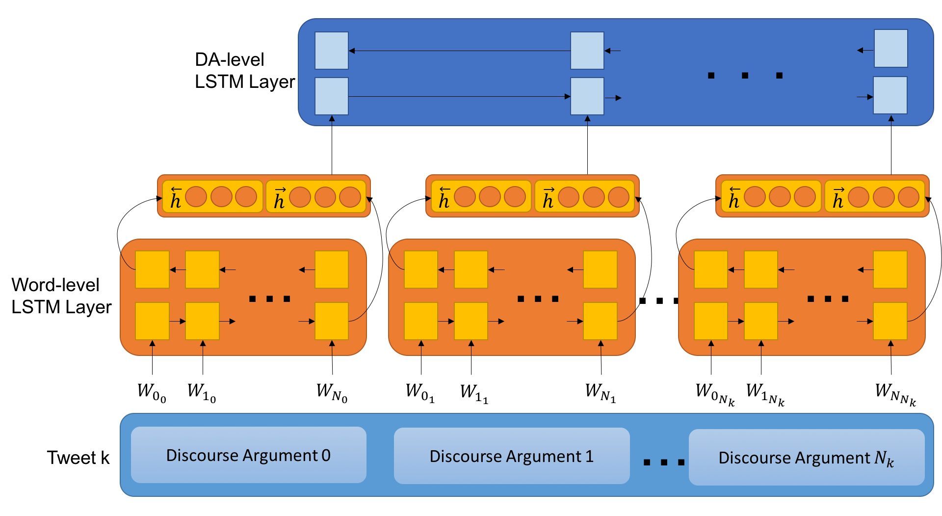
Figure 2: LSTM classifier for causality detection and explanation identification

Feature Based Models

We trained a linear SVM, an rbf SVM, and a random forest with N-gram, charater N-gram, and tweet POS tags, sentiment tags, average word lengths and word counts from each message as they have a pivotal role in the models for many NLP downstream tasks in social media Mohammad et al. (2013); Lynn et al. (2017). In addition to these features, we also extracted First-Last, First3 features and Word Pairs from every adjacent pair of discourse arguments since these features were most helpful for causal relation prediction Pitler et al. (2009). First-Last, First3 features are first and last word and first three words of two discourse arguments of the relation, and Word Pairs are the cross product of words of those discourse arguments. These two features enable our model to capture interaction between two discourse arguments. Pitler et al. (2009) reported that these two features along with verbs, modality, context, and polarity (which can be captured by N-grams, sentiment tags and POS tags in our previous features) obtained the best performance for predicting Contingency class to which causality belongs.

Recursive Neural Network Model

We load the GLOVE word embedding Pennington et al. (2014) trained in Twitter for each token of extracted discourse arguments from messages. For the distributional representation of discourse arguments, we run a Word-level LSTM on the words’ embeddings within each discourse argument and concatenate last hidden state vectors of forward LSTM ($\overrightarrow{h}$) and backward LSTM ($\overleftarrow{h}$) which is suggested by Ji and Smith (2017) ($DA=[\overrightarrow{h};\overleftarrow{h}]$). Then, we feed the sequence of the vector representation of discourse arguments to the Discourse-argument-level LSTM (DA-level LSTM) to make a final prediction with log softmax function. With this structure, the model can learn the representation of interaction of tokens inside each discourse argument, then capture discourse relations across all of the discourse arguments in each message (Figure 2). In order to prevent the overfitting, we added a dropout layer between the Word-level LSTM and the DA-level LSTM layer.

Architectural Variants

We also explore subsets of the full RNN architecture, specifically with one of the two LSTM layers removed. In the first model variant, we directly input all word embeddings of a whole message to a BiLSTM layer and make prediction (Word LSTM) without the help of the distributional vector representations of discourse arguments. In the second model variant, we take the average of all word embeddings of each discourse argument ($DA_{k}=\frac{1}{N_{k}}\sum_{i=1}^{N_{k}}W_{i}$), and use them as inputs to a BiLSTM layer (DA AVG LSTM) as the average vector of embeddings were quite effective for representing the whole sequence Ji and Smith (2017); Wieting et al. (2015). As with the full architectures, for CP both of these variants ends with a many-to-one classification per message, while the CEI model ends with a sequence of classifications.

3.3 Experiment

Feature Based Model

We explored three types of models (RBF SVM, Linear SVM, and Random Forest Classifier) which have previously been shown empirically useful for the language analysis in social media. We filtered out low frequency Word Pairs features as they tend to be noisy and sparse Pitler et al. (2009). Then, we conducted univariate feature selection to restrict all remaining features to those showing at least a small relationship with the outcome. Specifically, we keep all features passing a family-wise error rate of $\alpha=60$ with the given outcome. After comparing the performance of the optimized version of each model, we also conducted a feature ablation test on the best model in order to see how much each feature contributes to the causality prediction.

Neural Network Model

We used bidirectional LSTMs for causality classification and causal explanation identification since the discourse arguments for causal explanation can show up either before and after the effected events or results and we want our model to be optimized for both cases. However, there is a risk of overfitting due to the dataset which is relatively small for the high complexity of the model, so we added a dropout layer (p=0.3) between the Word-level LSTM and the DA-level LSTM.

For tuning our model, we explore the dimensionality of word vector and LSTM hidden state vectors of discourse arguments of 25, 50, 100, and 200 as pretrained GLOVE vectors were trained in this setting. For optimization, we used Stochastic Gradient Descent (SGD) and Adam Kingma and Ba (2014) with learning rates 0.01 and 0.001.

We ignore missing word embeddings because our dataset is quite small for retraining new word embeddings. However, if embeddings are extracted as separate discourse arguments, we used the average of all vectors of all discourse arguments in that message. Average embeddings have performed well for representing text sequences in other tasks Wieting et al. (2015).

Model Evaluation

We first use state-of-the-art PDTB taggers for our baseline Lin et al. (2014); Biran and McKeown (2015) for the evaluation of the causality prediction of our models (Biran and McKeown (2015) requires sentences extracted from the text as its input, so we used our parser to extract sentences from the message). Then, we compare how models work for each task and disassembled them to inspect how each part of the models can affect their final prediction performances. We conducted McNemar’s test to determine whether the performance differences are statistically significant at $p<.05$.

4 Results

We investigated various models for both causality detection and explanation identification. Based on their performances on the task, we analyzed the relationships between the types of models and the tasks, and scrutinized further for the best performing models. For performance analysis, we reported weighted F1 of classes.

4.1 Causality Prediction

Model	F1
Biran and McKeown (2015)	0.434
Lin et al. (2014)	0.638
Linear SVM	0.791
RBF SVM	0.777
Random Forest	0.771
LSTM	0.758

Table 3: Causality prediction performance across different predictive models. Bold indicates significant improvement over the LSTM

Model	F1
All	0.791
- First-Last, First3	0.788
- Word Pairs	0.787
- POS tags	0.734
- (Char + Word) N-grams	0.769
- Sentiment tags	0.791

Table 4: Feature ablation test of Linear SVM for causality prediction

In order to classify whether a message contains causal relation, we compared off-the-shelf PDTB parsers, linear SVM, RBF SVM, Random forest and LSTM classifiers. The off-the-shelf parsers achieved the lowest accuracies (Biran and McKeown (2015) and Lin et al. (2014) in Table 3). This result can be expected since 1) these models were trained with news articles and 2) they are trained for all possible discourse relations in addition to causal relations (e.g., contrast, condition, etc). Among our suggested models, SVM and random forest classifier performed better than LSTM and, in the general trend, the more complex the models were, the worse they performed. This suggests that the models with more direct and simpler learning methods with features might classify the causality messages better than the ones more optimized for capturing distributional information or non-linear relationships of features.

Causality Classifier Analysis

Table 4 shows the results of a feature ablation test to see how each feature contributes to causality classification performance of the linear SVM classifier. POS tags caused the largest drop in F1. We suspect POS tags played a unique role because discourse connectives can have various surface forms (e.g., because, cuz, bcuz, etc) but still the same POS tag ‘P’. Also POS tags can capture the occurrences of modal verbs, a feature previously found to be very useful for detecting similar discourse relations Pitler et al. (2009). N-gram features caused 0.022 F1 drop while sentiment tags did not affect the model when removed. Unlike the previous work where First-Last, First3 and Word pairs tended to gain a large F1 increase for multiclass discourse relation prediction, in our case, they did not affect the prediction performance compared to other feature types such as POS tags or N-grams.

4.2 Causal Explanation Identification

Model	Prec	Rec	F1
Linear SVM	0.773	0.727	0.743
RBF SVM	0.739	0.771	0.749
Random Forest	0.747	0.790	0.746
LSTM	0.851	0.858	0.853

Table 5: Causal explanation identification performance. Bold indicates significant imrpovement over next best model ($p<.05$)

In this task, the model identifies causal explanations given the discourse arguments of the causality message. We explored over the same models as those we used for causality (sans the output layer), and found the almost opposite trend of performances (see Table 5). The Linear SVM obtained lowest F1 while the LSTM model made the best identification performance. As opposed to the simple binary classification of the causality messages, in order to detect causal explanation, it is more beneficial to consider the relation across discourse arguments of the whole message and implicit distributional representation due to the implicit causal relations between two distant arguments.

4.3 Architectural Variants

Model	CP (F1)	CEI (F1)
Full LSTM	0.758	0.853
DA AVG LSTM	0.685	0.818
Word LSTM	0.694	0.792

Table 6: The effect of Word-level LSTM (Word LSTM) and discourse argument LSTM (DA AVG LSTM) for causality prediction (CP) and causal explanation identification (CEI). Note that, as described in methods, there are architectural differences for CP and CEI models with the same names, most notably that the output layer is always a single classification for CP and a sequence of classifications for CEI.

For causality prediction, we experimented with only word tokens in the whole message without help of Word-level LSTM layer (Word LSTM), and F1 dropped by 0.064 (CP in Table 6). Also, when we used the average of the sequence of word embeddings of each discourse argument as an input to the DA-level LSTM and it caused F1 drop of 0.073. This suggests that the information gained from both the interaction of words in and in between discourse arguments help when the model utilizes the distributional representation of the texts.

For causal explanation identification, in order to test how the LSTM classifier works without its capability of capturing the relations between discourse arguments, we removed DA-level LSTM layer and ran the LSTM directly on the word embedding sequence for each discourse argument for classifying whether the argument is causal explanation, and the model had 0.061 F1 drop (Word LSTM in CEI in Table 6). Also, when we ran DA-level LSTM on the average vectors of the word sequences of each discourse argument of messages, F1 decreased to 0.818. This follows the similar pattern observed from other types of models performances (i.e., SVMs and Random Forest classifiers) that the models with higher complexity for capturing the interaction of discourse arguments tend to identify causal explanation with the higher accuracies.

For CEI task, we found that when the model ran on the sequence representation of discourse argument (DA AVG LSTM), its performance was higher than the plain sequence of word embeddings (Word LSTM). Finally, in both subtasks, when the models ran on both Word-level and DA-Level (Full LSTM), they obtained the highest performance.

4.4 Complete Pipeline

Model	Prec	Rec	F1
CP + CEIcausal	0.864	0.877	0.868
CP + CEIall	0.842	0.864	0.848
CEIcausal Only	0.847	0.788	0.810
CEIall Only	0.836	0.848	0.842

Table 7: The effect of Linear SVM Cauality model (CP) within our pipeline. CEI_all: LSTM CEI models trained on all messages; CEI_causal: LSTM CEI models trained only on causality messages (CEI_causal); CP + CEI_all|causal: the combination of Linear SVM and each LSTM model. Bold: significant ($p<.05$) increase in F1 over the next best model, suggesting the two-step approach worked best.

Evaluations thus far zeroed-in on each subtask of causal explanation analysis (i.e. CEI only focused on data already identified to contain causal explanations). Here, we seek to evaluate the complete pipeline of CP and CEI, starting from all of test data (those or without causality) and evaluating the final accuracy of CEI predictions. This is intended to evaluate CEI performance under an applied setting where one does not already know whether a document has a causal explanation.

There are several approaches we could take to perform CEI starting from unannotated data. We could simply run CEI prediction by itself (CEI Only) or the pipeline of CP first and then only run CEI on documents predicted as causal (CP + CEI). Further, the CEI model could be trained only on those documents annotated causal (as was done in the previous experiments) or on all training documents including many that are not causal.

Table 7 show results varying the pipeline and how CEI was trained. Though all setups performed decent ($F1>0.81$) we see that the pipelined approach, first predicting causality (with the linear SVM) and then predicting causal explanations only for those with marked causal (CP + CEI_causal) yielded the strongest results. This also utilized the CEI model only trained on those annotated causal. Besides performance, an added benefit from this two step approach is that the CP step is less computational intensive of the CEI step and approximately 2/3 of documents will never need the CEI step applied.

Limitations.

We had an inevitable limitation on the size of our dataset, since there is no other causality dataset over social media and the annotation required an intensive iterative process. This might have limited performances of more complex models, but considering the processing time and the computation load, the combination of the linear model and the RNN-based model of our pipeline obtained both the high performance and efficiency for the practical applications to downstream tasks. In other words, it’s possible the linear model will not perform as well if the training size is increased substantially. However, a linear model could still be used to do a first-pass, computationally efficient labeling, in order to shortlist social media posts for further labeling from an LSTM or more complex model.

5 Exploration

Here, we explore the use of causal explanation analysis for downstream tasks. First we look at the relationship between use of causal explanation and one’s demographics: age and gender. Then, we consider their use in sentiment analysis for extracting the causes of polarity ratings. Research involving human subjects was approved by the University of Pennsylvania Institutional Review Board.

Demographic differences.

We first explored variance in number of causality posts by demographics. To do this, we used self-authored posts from a random 300 consenting-users of the MyPersonality dataset Kosinski et al. (2013). For each user we calculate a $cp\_ratio$, defined as the number of causality predicted posts divided by their total number of posts, indicating the percentage of their posts which include a causal explanation. We then correlated this ratio with real-valued age using Pearson correlation and looked the differences by dichotomous gender using Cohen’s d (the difference in standardized means; only binary gender was available). We found significant ($p<.05$) moderate-sized associations for both, indicating both older individuals and females were likely to use more causal explanations.

Causality in Sentiment Analysis

We explored the application of causality explanation identification for sentiment analysis using the Yelp polarity dataset Zhang et al. (2015). We randomly selected 10,000 of both positive and negative reviews and ran our complete pipeline on them to extract the causal explanations from the reviews. We then analyzed the ngrams from (a) causal explanation and (b) all other discourse arguments testing for associations with polarity. We used the a Bayesian interpretation of the log odds ratio using an informative dirichlet prior defined by Monroe et al. (2008). We found difference in the top ngrams depending on whether the argument the ngram originated from was a causal explanation or not (see Table 8). Top ngrams for causal explanations included more content words (e.g. ‘rude’, ‘overpriced’, ‘slow’) suggesting analyzing causal explanations within reviews can better target the reasons for the negative review.

	CE	Non-CE
	Top Ngrams	Top Ngrams
1	worst	not
2	was	no
3	not	”
4	the worst	asked
5	horrible	she
6	rude	told
7	bad	said
8	overpriced	minutes
9	over	?
10	slow	me

Table 8: Top words most associated with negative reviews from within causal explanations (CE) and outside of causal explanation (Non-CE).

6 Conclusion

We developed a pipeline for causal explanation analysis over social media text, including both causality prediction and causal explanation identification. We examined a variety of model types and RNN architectures for each part of the pipeline, finding an SVM best for causality prediction and a hierarchy of BiLSTMs for causal explanation identification, suggesting the later task relies more heavily on sequential information. In fact, we found replacing either layer of the hierarchical LSTM architecture (the word-level or the DA-level) with a an equivalent “bag of features” approach resulted in reduced accuracy. Results of our whole pipeline of causal explanation analysis were found quite strong, achieving an $F1=0.868$ at identifying discourse arguments that are causal explanations.

Finally, we demonstrated use of our models in applications, finding associations between demographics and rate of mentioning causal explanations, as well as showing differences in the top words predictive of negative ratings in Yelp reviews. Utilization of discourse structure in social media analysis has been a largely untapped area of exploration, perhaps due to its perceived difficulty. We hope the strong results of causal explanation identification here leads to the integration of more syntax and deeper semantics into social media analyses and ultimately enables new applications beyond the current state of the art.

References

- Bhatia et al. (2015) Parminder Bhatia, Yangfeng Ji, and Jacob Eisenstein. 2015. Better document-level sentiment analysis from rst discourse parsing. arXiv preprint arXiv:1509.01599.
- Biran and McKeown (2015) Or Biran and Kathleen McKeown. 2015. Pdtb discourse parsing as a tagging task: The two taggers approach. In Proceedings of the 16th Annual Meeting of the Special Interest Group on Discourse and Dialogue, pages 96–104.
- Carver and Gaines (1987) Charles S Carver and Joan Gollin Gaines. 1987. Optimism, pessimism, and postpartum depression. Cognitive therapy and Research, 11(4):449–462.
- Feng and Hirst (2014) Vanessa Wei Feng and Graeme Hirst. 2014. A linear-time bottom-up discourse parser with constraints and post-editing. In Proceedings of the 52nd Annual Meeting of the Association for Computational Linguistics (Volume 1: Long Papers), volume 1, pages 511–521.
- Ji and Eisenstein (2014) Yangfeng Ji and Jacob Eisenstein. 2014. Representation learning for text-level discourse parsing. In ACL (1), pages 13–24.
- Ji and Smith (2017) Yangfeng Ji and Noah Smith. 2017. Neural discourse structure for text categorization. arXiv preprint arXiv:1702.01829.
- Kingma and Ba (2014) Diederik P Kingma and Jimmy Ba. 2014. Adam: A method for stochastic optimization. arXiv preprint arXiv:1412.6980.
- Kong et al. (2014) Lingpeng Kong, Nathan Schneider, Swabha Swayamdipta, Archna Bhatia, Chris Dyer, and Noah A Smith. 2014. A dependency parser for tweets.
- Kosinski et al. (2013) Michal Kosinski, David Stillwell, and Thore Graepel. 2013. Private traits and attributes are predictable from digital records of human behavior. Proceedings of the National Academy of Sciences, 110(15):5802–5805.
- Li et al. (2014) Jiwei Li, Rumeng Li, and Eduard Hovy. 2014. Recursive deep models for discourse parsing. In Proceedings of the 2014 Conference on Empirical Methods in Natural Language Processing (EMNLP), pages 2061–2069.
- Lin et al. (2014) Ziheng Lin, Hwee Tou Ng, and Min-Yen Kan. 2014. A pdtb-styled end-to-end discourse parser. Natural Language Engineering, 20(02):151–184.
- Lynn et al. (2017) Veronica Lynn, Youngseo Son, Vivek Kulkarni, Niranjan Balasubramanian, and H Andrew Schwartz. 2017. Human centered nlp with user-factor adaptation. In Proceedings of the 2017 Conference on Empirical Methods in Natural Language Processing, pages 1146–1155.
- Mann and Thompson (1987) William C Mann and Sandra A Thompson. 1987. Rhetorical structure theory: A theory of text organization. University of Southern California, Information Sciences Institute.
- Mohammad et al. (2013) Saif M Mohammad, Svetlana Kiritchenko, and Xiaodan Zhu. 2013. Nrc-canada: Building the state-of-the-art in sentiment analysis of tweets. arXiv preprint arXiv:1308.6242.
- Monroe et al. (2008) Burt L Monroe, Michael P Colaresi, and Kevin M Quinn. 2008. Fightin’words: Lexical feature selection and evaluation for identifying the content of political conflict. Political Analysis, 16(4):372–403.
- Park and Cardie (2012) Joonsuk Park and Claire Cardie. 2012. Improving implicit discourse relation recognition through feature set optimization. In Proceedings of the 13th Annual Meeting of the Special Interest Group on Discourse and Dialogue, pages 108–112. Association for Computational Linguistics.
- Paulus et al. (2014) Romain Paulus, Richard Socher, and Christopher D Manning. 2014. Global belief recursive neural networks. In Advances in Neural Information Processing Systems, pages 2888–2896.
- Pennington et al. (2014) Jeffrey Pennington, Richard Socher, and Christopher D. Manning. 2014. Glove: Global vectors for word representation. In Empirical Methods in Natural Language Processing (EMNLP), pages 1532–1543.
- Peterson et al. (1988) Christopher Peterson, Martin E Seligman, and George E Vaillant. 1988. Pessimistic explanatory style is a risk factor for physical illness: a thirty-five-year longitudinal study. Journal of personality and social psychology, 55(1):23.
- Pitler et al. (2009) Emily Pitler, Annie Louis, and Ani Nenkova. 2009. Automatic sense prediction for implicit discourse relations in text. In Proceedings of the Joint Conference of the 47th Annual Meeting of the ACL and the 4th International Joint Conference on Natural Language Processing of the AFNLP: Volume 2-Volume 2, pages 683–691. Association for Computational Linguistics.
- Pitler and Nenkova (2009) Emily Pitler and Ani Nenkova. 2009. Using syntax to disambiguate explicit discourse connectives in text. In Proceedings of the ACL-IJCNLP 2009 Conference Short Papers, pages 13–16. Association for Computational Linguistics.
- Prasad et al. (2007) Rashmi Prasad, Eleni Miltsakaki, Nikhil Dinesh, Alan Lee, Aravind Joshi, Livio Robaldo, and Bonnie L Webber. 2007. The penn discourse treebank 2.0 annotation manual.
- Scheier et al. (1989) Michael F Scheier, Karen A Matthews, Jane F Owens, George J Magovern, R Craig Lefebvre, R Anne Abbott, and Charles S Carver. 1989. Dispositional optimism and recovery from coronary artery bypass surgery: the beneficial effects on physical and psychological well-being. Journal of personality and social psychology, 57(6):1024.
- Son et al. (2017) Youngseo Son, Anneke Buffone, Joe Raso, Allegra Larche, Anthony Janocko, Kevin Zembroski, H Andrew Schwartz, and Lyle Ungar. 2017. Recognizing counterfactual thinking in social media texts. In Proceedings of the 55th Annual Meeting of the Association for Computational Linguistics (Volume 2: Short Papers), volume 2, pages 654–658.
- Wieting et al. (2015) John Wieting, Mohit Bansal, Kevin Gimpel, and Karen Livescu. 2015. Towards universal paraphrastic sentence embeddings. arXiv preprint arXiv:1511.08198.
- Zhang et al. (2015) Xiang Zhang, Junbo Zhao, and Yann LeCun. 2015. Character-level convolutional networks for text classification. In Advances in neural information processing systems, pages 649–657.
- Zhou et al. (2010) Zhi-Min Zhou, Yu Xu, Zheng-Yu Niu, Man Lan, Jian Su, and Chew Lim Tan. 2010. Predicting discourse connectives for implicit discourse relation recognition. In Proceedings of the 23rd International Conference on Computational Linguistics: Posters, pages 1507–1514. Association for Computational Linguistics.