Random Language Model

Abstract

Many complex generative systems use languages to create structured objects. We consider a model of random languages, defined by weighted context-free grammars. As the distribution of grammar weights broadens, a transition is found from a random phase, in which sentences are indistinguishable from noise, to an organized phase in which nontrivial information is carried. This marks the emergence of deep structure in the language, and can be understood by a competition between energy and entropy.

It is a remarkable fact that structures of the most astounding complexity can be encoded into sequences of digits from a finite alphabet. Indeed, the complexity of life is written in the genetic code, with alphabet $\{A,T,C,G\}$, proteins are coded from strings of 20 amino acids, and human-written text is composed in small, fixed alphabets. This ‘infinite use of finite means’ Von Humboldt (1999) was formalized by Post and Chomsky with the notion of generative grammar Post (1943); Chomsky (2002), and has been elaborated upon since, both by linguists and computer scientists Hopcroft et al. (2007). A generative grammar consists of an alphabet of hidden symbols, an alphabet of observable symbols, and a set of rules, which allow certain combinations of symbols to be replaced by others. From an initial start symbol $S$, one progressively applies the rules until only observable symbols remain; any sentence produced this way is said to be ‘grammatical,’ and the set of all such sentences is called the language of the grammar. The sequence of rule applications is called a derivation. For example, the grammar $\{S\to SS,S\to(S),S\to()\}$ has a single hidden symbol $S$ and two observable symbols, $($ and $)$, and produces the infinite set of all strings of well-formed parentheses. A simple derivation in this grammar is $S\to SS\to(S)S\to(())S\to(())()$. Besides their original use in linguistics, where the observable symbols are typically taken to be words, and grammars produce sentences (Fig 1a) Chomsky (2002, 2014), generative grammars have found application in manifold domains: in the secondary structure of RNA (Fig 1b) Searls (2002); Knudsen and Hein (2003), in compiler design Hopcroft et al. (2007), in self-assembly Winfree et al. (1999), in protein sequence analysis Barton et al. (2016), and in quasicrystals Escudero (1997), to name a few.

Figure 1: Illustrative derivation trees for (a) simple English sentence, and (b) RNA secondary structure (after Searls (2002)). The latter is a derivation of the sequence ‘gacuaagcugaguc’ and shows its folded structure. Terminal symbols are encircled.

The complexity of a language is limited by conditions imposed on its grammar, as described by the Chomsky hierarchy, which, in increasing complexity, distinguishes regular, context-free, context-sensitive, and recursively enumerable grammars Nowak et al. (2002). Each class of grammar has a characteristic graphical structure of its derivations: regular grammars produce linear derivations, context-free grammars produce trees (Fig 1), and context-sensitive and recursively enumerable grammars produce more elaborate graphs. Associated with an increase in complexity is an increased difficulty of parsing Hopcroft et al. (2007). Because biological instantiations of grammars must have been discovered by evolution, there is a strong bias toward simpler grammars; we consider context-free grammars (CFGs), which are the lowest order of the Chomsky hierarchy that supports hierarchical structure.

Despite their ubiquity in models of complex generative systems, grammars have hitherto played a minor role in physics, and most known results on grammars are theorems regarding worst-case behavior , which need not represent the typical case. Human languages show Zipf’s law Zipf (2013); i Cancho and Solé (2003); Corral et al. (2015), a power-law dependence of word frequency on its rank, and many sequences, including human text, show long-range information-theoretic correlations Ebeling and Pöschel (1994); Schürmann and Grassberger (1996); Lin and Tegmark (2017), which can be created by a CFG Lin and Tegmark (2017); but are these typical features of some ensemble of grammars? In this work we initiate this research program by proposing and simulating an ensemble of CFGs, so that grammars can be considered as physical systems Parisi (1999). We will find that CFGs possess two natural ‘temperature’ scales that control grammar complexity, one at the surface interface, and another in the tree interior. As either of these temperatures is lowered, there is a phase transition, which corresponds to the emergence of nontrivial information propagation. We characterize this phase transition using results from simulations, and understand its location by a balance between energy and entropy.

Generative grammars: A generative grammar is defined by an alphabet $\chi$ and a set of rules $\mathcal{R}$. The alphabet has $N$ hidden, ‘non-terminal’ symbols $\chi_{H}$, and $T$ observable, ‘terminal’ symbols $\chi_{O}$. The most general rule is of the form $a_{1}a_{2}\ldots a_{n}\to b_{1}b_{2}\ldots b_{m}$, where $a_{i}\in\chi_{H},b_{i}\in\chi=\chi_{H}\cup\chi_{O}$. In a CFG the rules are specialized to the form $a_{1}\to b_{1}b_{2}\ldots b_{m}$, and we will insist that $m\geq 1$, so that there is no ‘empty’ string. Without loss of generality, we consider CFGs in Chomsky normal form, in which case all rules are of the form Hopcroft et al. (2007) $a\to b\;c$ or $a\to A$, where $a,b,c\in\chi_{H}$ and $A\in\chi_{O}$. Note that we may have $b=a$, or $b=c$, or $a=b=c$. Any derivation in Chomsky reduced form can be drawn on a binary tree. Beginning from the start symbol $S\in\chi_{H}$, rules are applied until the string contains only observable symbols. Such a string is called a sentence. The set of all sentences is the language of the grammar. Given a string of observables $\mathcal{S}=A_{1}\ldots A_{\ell}$ and a grammar $\mathcal{G}$, one can ask whether there exists a derivation that produces $\mathcal{S}$ from the start symbol $S$; if so, $\mathcal{S}$ is said to be grammatical.

A formal grammar as defined above can only distinguish grammatical from ungrammatical sentences. A richer model is obtained by giving each rule a non-negative real valued weight. Such a weighted grammar is useful in applications, because weights can be continuously driven by a learning process, and can be used to define probabilities of parses. Moreover, a weighted grammar can be put into the Gibbs form, as shown below. For CFGs, to every rule of the form $a\to bc$ we assign a weight $M_{abc}$, and to every rule of the form $a\to A$ we assign a weight $O_{aA}$.

Each candidate derivation of a sentence has two different types of degrees of freedom. There is the topology $\mathcal{T}$ of the tree, namely the identity (terminal or non-terminal) of each node, as well as the variables, both terminal and non-terminal, on the nodes. We write $\Omega_{\mathcal{T}}$ for the set of internal factors, i.e. factors of the form $a\to bc$, and $\partial\Omega_{\mathcal{T}}$ for the boundary factors, i.e. those associated to $a\to A$ rules. The number of boundary factors is written $\ell_{\mathcal{T}}$, which is also the number of leaves. Since derivations are trees, the number of internal factors is $\ell_{\mathcal{T}}-1$. We will write $\sigma$ for non-terminal symbols, and $o$ for terminals; these can be enumerated in an arbitrary way $1,\ldots,N$ and $1,\ldots,T$, respectively. Given $\mathcal{T}$, we can write $\sigma_{i}$ for the value of the non-terminal on site $i$, and similarly $o_{j}$ for the terminal on site $j$. The number of $\sigma_{i}$ is $2\ell_{\mathcal{T}}-1$, while the number of $o_{j}$ is $\ell_{\mathcal{T}}$. We write $\mathcal{G}$ for the pair $M,O$, $\sigma$ for $\{\sigma_{i}\}$, and $o$ for $\{o_{t}\}$.

To define a probability measure on derivations, it is convenient to factorize it into the part specifying $\mathcal{T}$, and the remainder. In this way we separate the the tree shape from the influence of the grammar on variables. For a fixed $\mathcal{T}$ the weight of a configuration is

$$W(\sigma,o|\mathcal{T},\mathcal{G})=\prod_{\alpha\in\Omega_{\mathcal{T}}}M_{\sigma_{\alpha_{1}}\sigma_{\alpha_{2}}\sigma_{\alpha_{3}}}\prod_{\alpha\in\partial\Omega_{\mathcal{T}}}O_{\sigma_{\alpha_{1}}o_{\alpha_{2}}},$$ (1)

where each $\alpha=(\alpha_{1},\alpha_{2},\alpha_{3})$ is a factor in the order $\sigma_{\alpha_{1}}\to\sigma_{\alpha_{2}}\sigma_{\alpha_{3}}$. Note that $M_{abc}\neq M_{acb}$ in general, thus the left and right branches are distinguished . We can write $W=e^{-E}$ with

$$E=-\sum_{a,b,c}\pi_{abc}(\sigma)\log M_{abc}-\sum_{a,B}\rho_{aB}(\sigma,o)\log O_{aB}$$ (2)

where $\pi_{abc}$ is the number of times the rule $a\to bc$ appears in the configuration $\sigma$, and likewise $\rho_{aB}$ is the number of times the rule $a\to B$ appears. This defines a conditional probability measure on configurations $\mathbb{P}(\sigma,o|\mathcal{T},\mathcal{G})~{}=~{}e^{-E(\sigma,o|\mathcal{T},\mathcal{G})}/Z(\mathcal{T},\mathcal{G})$ where

$$Z(\mathcal{T},\mathcal{G})=\sum_{\{\sigma_{i},o_{t}\}}e^{-E(\sigma,o|\mathcal{T},\mathcal{G})}.$$ (3)

All configurations have $S$ at the root node. For simplicity, in this work we consider as a model for the tree topology probability $\mathbb{P}(\mathcal{T}|\mathcal{G})=W_{tree}/Z_{tree}$ with $W_{tree}(\mathcal{T})=p^{|\partial\Omega_{\mathcal{T}}|}(1-p)^{|\Omega_{\mathcal{T}}|}$, where $p$ is the emission probability, the probability that a hidden node becomes an observable node. $p$ controls the size of trees; we will choose it such that the tree size distribution is cutoff above a length $\xi=1000$. Some facts about the resulting binary trees are recorded in Supplementary Material .

A model with weights of the form (1) is called a weighted CFG (WCFG). In the particular case where $1=\sum_{b,c}M_{abc}=\sum_{A}O_{aA}$ for all $a$, it is easy to see that $M$ and $O$ are conditional probabilities: $M_{abc}=\mathbb{P}(a\to bc\;|\;a\to\mbox{non-terminal})$ and $O_{aA}=\mathbb{P}(a\to A\;|\;a\to\mbox{terminal})$. In this case the model is called a probabilistic CFG (PCFG). In the main text, we consider a weighted CFG, model W; in SI, we show that our results are robust in model P, a PCFG. There are tradeoffs between these models: model P is easier to sample, because it has $Z(\mathcal{T},\mathcal{G})=1$ from normalization of probability, and thus is factorized. But model W is more amenable to theory, since it is less constrained.

Random Language Model: Each grammar defines probabilities for sentences. To extract the universal properties of grammars, which do not depend on all details of $M$ and $O$, we need a measure on the space of grammars. What is an appropriate measure? From Eq.(2), $\log M$ and $\log O$ are analogous to coupling constants in statistical mechanics. A simple model is to assume a Gaussian distribution for these, so that $M$ and $O$ are lognormal. This can be motivated as follows: language evolution is a dynamical process, which must be slow in order for language to remain comprehensible at any given moment. If each $\log M_{abc}$ and $\log O_{aB}$ are the accumulation of independent, additive increments Sornette and Cont (1997), these will lead to a lognormal. We define deep and surface sparsities as, respectively,

$$s_{d}=\frac{1}{N^{3}}\sum_{a,b,c}\log^{2}\left[\frac{M_{abc}}{\overline{M}}\right],\;\;s_{s}=\frac{1}{NT}\sum_{a,B}\log^{2}\left[\frac{O_{aB}}{\overline{O}}\right]$$ (4)

where $\overline{M}=1/N^{2}$ and $\overline{O}=1/T$ are the corresponding uniform probabilities; it is convenient to use this normalization even for model W where weights are not strictly normalized. A lognormal distribution of grammar weights is

$$\mathbb{P}_{G}(M,O) \equiv Z_{G}^{-1}\;J\;e^{-\epsilon_{d}s_{d}}e^{-\epsilon_{s}s_{s}}$$ (5)

where $J=e^{-\sum_{a,b,c}\log M_{abc}-\sum_{a,B}\log O_{aB}}$, and the space of $M$ and $O$ is defined by appropriate normalization and positivity constraints. We define the Random Language Model as the ensemble of grammars drawn from Eq.5.

An alternative motivation of (5) is that this is the maximum-entropy measure when the grammar-averages $\overline{s_{d}}$ and $\overline{s_{s}}$ are constrained. $s_{d}$ and $s_{s}$ measure the density of rules about their respective median values $\overline{M}$ and $\overline{O}$. When $s_{d}$ and $s_{s}$ are finite, all rules must have a finite probability: this reflects the fact that, given any finite amount of data, one can only put a lower bound on the probability of any particular rule. In model W the Lagrange multipliers $\epsilon_{d}$ and $\epsilon_{s}$ satisfy

$$\overline{s_{d}}=\frac{N^{3}}{2\epsilon_{d}},\qquad\overline{s_{s}}=\frac{NT}{2\epsilon_{s}}.$$ (6)

When $\epsilon_{d}\to\infty$, $\overline{s_{d}}\to 0$, which is the value corresponding to a completely uniform deep grammar, that is, when for a non-terminal $a$, all rules $a\to bc$ have the same probability $1/N^{2}$. This is clearly the limit in which the grammar carries no information. As $\epsilon_{d}$ is lowered, $s_{d}$ increases, and the grammar carries more information. In terms of how deterministic the rules are, $\epsilon_{d}$ plays the role of temperature, with random $\leftrightarrow$ hot and deterministic $\leftrightarrow$ cold; we will refer to it as the deep temperature. This analogy can also be seen formally: in SI, we show that if the energy $E$ is replaced by $\beta E$, then (6) is replaced by $\overline{s_{d}}=\beta^{2}N^{3}/(2\epsilon_{d})$, such that lowering $\epsilon_{d}$ is equivalent to increasing $\beta$. Similarly, $\epsilon_{s}$ controls information transmission at the surface; we call it the surface temperature.

To investigate the role of $\epsilon_{d}$ on language structure, we sampled grammars from the RLM at fixed values $T=27,\epsilon_{s}/(NT)=0.01$. Since the surface sparsity is large, there is already some simple structure at the surface; we will explore how deep structure emerges as $N$ and $\epsilon_{d}$ are varied. For each value of $N$ and $\epsilon_{d}$, we created 120 distinct grammars, from which we sample 200 sentences (see SI for more details). Altogether approximately 7200 distinct languages were constructed.

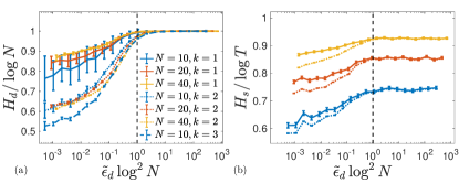
Figure 2: Shannon entropy of random CFGs as functions of $\tilde{\epsilon}_{d}=\epsilon_{d}/N^{3}$. (a) Block entropy of hidden configurations for indicated $k$ and $N$. (b) Block entropy of observed strings; symbols as in (a). The constant value for $\epsilon_{d}>\epsilon_{*}$ depends on the surface temperature $\epsilon_{s}$. Bars indicate $20^{th}$ and $80^{th}$ percentiles.

The information content of a grammar $\mathcal{G}$ is naturally encoded by Shannon entropies. For a sequence $o_{1},o_{2},\ldots,o_{k}$ the Shannon block entropy rate is

$$H_{s}(\mathcal{G};k)=\frac{1}{k}\big{\langle}\log 1/\mathbb{P}(o_{1},o_{2},\ldots,o_{k}|\mathcal{G})\big{\rangle}$$ (7)

For CFGs we can also consider the block entropy rate of deep configurations,

$$H_{d}(\mathcal{G};k)=\frac{1}{k}\big{\langle}\log 1/\mathbb{P}(\sigma_{1},\sigma_{2},\ldots,\sigma_{k}|\mathcal{G})\big{\rangle}$$ (8)

where the symbols are taken from a (leftmost) derivation. In both cases the ensemble average is taken with the actual probability of occurrence, $\mathbb{P}(o|\mathcal{G})$ for $H_{s}$, and $\mathbb{P}(\sigma|\mathcal{G})$ for $H_{d}$.

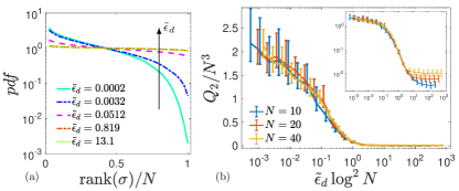
Figure 3: (a) Zipf plot of hidden symbols for $N=40$. Here $\tilde{\epsilon}_{d}=\epsilon_{d}/N^{3}$. (b) Order parameter $Q_{2}$, with bars indicating $20^{th}$ and $80^{th}$ percentile ranges over grammars at each parameter value. Inset: same plot in log-log axes.

The grammar averages $\overline{H}_{d}(k)$ and $\overline{H}_{s}(k)$ are shown in Fig. 2, for $k$ as indicated; here and in the following, the bars show the $20^{th}$ and $80^{th}$ percentiles, indicating the observable range of $H_{d}$ and $H_{s}$ over the ensemble of grammars . The dependence on $\epsilon_{d}$ is striking: for $\epsilon_{d}\gtrsim N^{3}/\log^{2}N$, both $\overline{H}_{s}(1)$ and $\overline{H}_{d}(1)$ are flat. In this regime, $\overline{H}_{d}(1)\approx\log N$, indicating that although configurations strictly follow the rules of a WCFG, deep configurations are nearly indistinguishable from completely random configurations. However, at $\epsilon_{d}=\epsilon_{*}\approx N^{3}/\log^{2}N$ there is a pronounced transition, and both entropies begin to drop. This transition corresponds to the emergence of deep structure.

The first block entropy $H_{d}(\mathcal{G};1)$ measures information in the single-character distribution, while the differential entropies $\delta H_{d}(\mathcal{G};k)=(k+1)H_{d}(\mathcal{G};k+1)-kH_{d}(\mathcal{G};k)$ measure incremental information in the higher-order distributions Schürmann and Grassberger (1996). The Shannon entropy rate including all correlations can either be obtained from $\lim_{k\to\infty}H_{d}(\mathcal{G};k)$, or from $\lim_{k\to\infty}\delta H_{d}(\mathcal{G};k)$. These coincide, but the latter converges faster Schürmann and Grassberger (1996). In SI, we show that $\delta H_{d}(\mathcal{G};k)$, and thus the limiting rate, appears to collapse with $\tilde{\epsilon}_{d}\log N$. For all entropies the sample-to-sample fluctuations decrease rapidly with $k$, suggesting that the limiting rates are self-averaging.

To further investigate the nature of the transition, we show in Fig. 3a a Zipf plot: the frequency of each symbol, arranged in decreasing order. Fig. 3a shows the Zipf plot for deep structure; the Zipf plot for surface structure is similar, but less dramatic (see SI). We see a sharp change at $\epsilon_{*}$: for $\epsilon_{d}>\epsilon_{*}$, the frequencies of hidden symbols are nearly uniform, while below $\epsilon_{*}$, the distribution is closer to exponential ( In SI, we show that a power-law regime for the observable symbols appears when $T$ is large). The permutation symmetry among hidden symbols is thus spontaneously broken at $\epsilon_{*}$.

What is the correct order parameter to describe this transition? The ferromagnetic order parameter is $m_{r}=\overline{\langle N\delta_{\sigma_{i},r}-1\rangle}$, where $i$ is a site. This does not show any signal of a transition, despite the fact that the start symbol explicitly breaks the replica symmetry. A more interesting choice is one of Edwards-Anderson type, such as $Q^{EA}_{rs}=\overline{\langle N\delta_{\sigma_{i},r}-1\rangle\langle N\delta_{\sigma_{i},s}-1\rangle}$ where $r$ and $s$ label different sentences produced from the same grammar, and $\sigma_{i}$ is a specified site Gross et al. (1985). However, sentences produced by a CFG do not have fixed derivation trees, so we need to compare symbols in relative position. For each interior rule $a\to bc$ we can define

$$Q_{abc}(\mathcal{G})=\langle\delta_{\sigma_{\alpha_{1}},a}\big{(}N^{2}\delta_{\sigma_{\alpha_{2}},b}\delta_{\sigma_{\alpha_{3}},c}-1\big{)}\rangle,$$ (9)

averaged over all interior vertices $\alpha$, and averaged over derivations. Here $\sigma_{\alpha_{1}}$ is the head symbol at vertex $\alpha$, and $\sigma_{\alpha_{2}},\sigma_{\alpha_{3}}$ are the left and right symbols, respectively. $Q$ measures patterns in rule application at each branching of a derivation tree. It is thus an order parameter for deep structure. Upon averaging over grammars in the absence of any fields, the permutation symmetry must be restored: $\overline{Q}_{abc}=q_{0}+\delta_{ab}\;q_{l}+\delta_{ac}\;q_{r}+\delta_{bc}\;q_{h}+\delta_{ab}\delta_{ac}\;q_{*}$. As shown in SI, these components show a transition, but there is significant noise below $\epsilon_{*}$, despite there being $120$ replicas at each point. Evidently, $Q_{abc}$ has large fluctuations below $\epsilon_{*}$. This suggests a definition $Q_{2}\equiv\overline{\sum_{a,b,c}Q_{abc}^{2}},$ plotted in Fig 3b. The signal is clear: on the large scale, $Q_{2}$ has a scaling form $Q_{2}\approx N^{3}f\left(\epsilon_{N}/\epsilon_{*}\right)$ and is small above $\epsilon_{*}$. The scaling $Q_{2}\sim N^{3}$ suggests that below the transition, all hidden symbols start to carry information in the deep structure.

Theory: How can we gain some theoretical insight into the RLM? Consider the entropy of an observed string of length $\ell$, composed of $n$ sentences of length $\ell_{k},\sum_{k}\ell_{k}=\ell$. The entropy of this string derives from 3 distinct combinatorial levels: (i) each sentence can be represented by a derivation tree with many different topologies; (ii) each derivation tree can host a variety of internal hidden variables; and (iii) given the hidden variables, the observed symbols can themselves vary.

Some scaling considerations are useful. Each derivation tree can have many topologies: the entropy of binary trees scales as $\ell_{k}\log 4$, so that the total tree entropy scales as $S_{t}\sim\ell\log 4$. Each derivation tree has $2\ell_{k}-1$ hidden variables, so that the total number of hidden DOF is $2\ell-n$, and the corresponding deep entropy scales as $S_{d}\sim(2\ell-n)\log N$. Finally, the sentences have an entropy $S_{o}\sim\ell\log T$.

We see that when typical sentences are of length $\langle\ell\rangle\gg 1$, so that $\ell-n\sim\ell$, these numbers are independent of partitioning, to leading order. For large $\langle\ell\rangle$ we get the scaling $S\sim\ell\log(4N^{2}T)$.

This must be compared with the ‘energetic’ terms $\log W_{tree}=(\ell-n)\log(1-p)+\ell\log p\sim-2\ell\log 2$ for $p$ near $1/2$, and $E$, Eq.(2). In $E$, $\pi$ is positively correlated with $M$, since rules with a higher weight are more frequently used; hence we can obtain a simple scaling estimate $E\sim-N^{3}\pi\log m-NT\rho\log o$ where $\pi$ is the mean value of $\pi_{abc}$, and $\log m$ is the value of a typical positive fluctuation of $\log M_{abc}$, and similarly for $O$. From the sum rules $\sum_{a,b,c}\pi_{abc}=|\Omega|=\ell-n$ and $\sum_{a,B}\rho_{aB}=|\partial\Omega|=\ell$ we have $\pi=(\ell-n)/N^{3},\rho=\ell/(NT)$. The mean value of $\log M_{abc}$ is $\log\overline{M}$, and the mean value of $\log O_{aB}$ is $\log\overline{O}$. These contributions lead to a constant value of $E$. The positive fluctuations in $\log M$ and $\log O$ that couple to $E$ scale as $\sqrt{\frac{N^{3}}{2\epsilon_{d}}}$ and $\sqrt{\frac{NT}{2\epsilon_{s}}}$, respectively, leading to

$$E\sim-\ell\sqrt{\frac{N^{3}}{2\epsilon_{d}}}-\ell\sqrt{\frac{NT}{2\epsilon_{s}}}+\mbox{const}$$ (10)

Combining this with $S$, the effective free energy $F=E-\log W_{tree}-S$ reflects a competition between energy and entropy. If we consider $N$ and $\epsilon_{d}$ as varying, then there is a scale $\epsilon_{*}=N^{3}/\log^{2}N$ where the energetic fluctuations balance entropy. For $\epsilon_{d}\gg\epsilon_{*}$, the energy of a configuration is unimportant, and the grammar is thus irrelevant: the language produced by the WCFG must then be indistinguishable from random sequences, as found empirically above. In contrast, for $\epsilon_{d}\ll\epsilon_{*}$, the language reflects those sequences with high intrinsic weight, and their entropy is less important. The characteristic scale $\epsilon_{*}$ identified by these simple arguments agrees with that found empirically above, and locates the emergence of deep structure. However, further work is needed to predict the behavior of $Q_{2}$, $H_{s}$, and $H_{d}$.

Learning human languages: Around 6000 languages are spoken around the world Baker (2008); given fractured and highly sparse input, how does a child come to learn the precise syntax of one of these many languages? This question has a long history in linguistics and cognitive science Berwick et al. (2011); Yang et al. (2017). One scenario for learning is known as the Principles and Parameters (P&P) theory Chomsky (1993). This posits that the child is biologically endowed with a general class of grammars, the ‘principles,’ and by exposure to one particular language, fixes its syntax by setting some number of parameters, assumed to be binary. For example, the head-directionality parameter controls whether verbs come before or after objects, like English and Japanese, respectively. A vast effort has been devoted to mapping out the possible parameters of human languages Baker (2008); Shlonsky (2010). The richness of the discovered structure has been used as criticism of the approach Ramchand and Svenonius (2014): if the child needs to set many parameters, then do these all need to be innate? This would be a heavy evolutionary burden, and a challenge to efficient learning.

The RLM can shed some light on this debate. First, since only 2 living human languages are known to possess syntax beyond CFG , we consider WCFGs a valid starting point . Following experimental work Yang et al. (2017), we picture the learning process as follows. Initially, the child does not know the rules of the grammar, so it begins with some small number of hidden symbols and assigns uniform values to the weights $M$ and $O$. To learn is to increase the likelihood of the grammar by adjusting the weights and adding new hidden symbols. As weights are driven away from uniform values, the temperatures $\epsilon_{d}$ and $\epsilon_{s}$ decrease. Eventually the transition to deep structure is encountered, and the grammar begins to carry information.

In the absence of any bias, this transition would occur suddenly and dramatically, spontaneously breaking all $N^{3}$ directions in $M$ space simultaneously, as in Fig. 3b. However, in realistic child language learning, the child’s environment acts as a field on this likelihood-ascent, and can cause the structure-emerging transitions to occur at different critical deep temperatures, depending on their coupling to the field. For example, a left-right symmetry breaking could correspond to setting the head directionality parameter.

Although this description is schematic, we insist that the various symmetry-breaking transitions, which could give rise to parameters, are emergent properties of the model. Thus if there are indeed many parameters to be set, these do not all need to be innate: the child only needs the basic structure of a WCFG, and the rest is emergent. The P&P theory is thus consistent with existence of many parameters. If the RLM can be solved, by which we mean that the partition function $Z$ can be computed, then the series of symmetry-breaking transitions that occur in the presence of a field can be inferred, and a map of syntax in CFGs could be deduced. This is a tantalizing goal for future work.

Conclusion: We introduced a model of random languages, which captures the generative aspect of complex systems. The model has a transition in parameter space that corresponds to the emergence of deep structure. Since the interaction is long-range, we expect that the RLM, or a variant, is exactly solvable. We hope that this will be clarified in the future.